DNN for HD-UQ

Talk given at SIAM annual meeting 2017 conference.

Transcript

1. DNN for High-D UQ with a simple extension to the multifidelity case Rohit Tripathy and Ilias Bilionis Predictive Science Lab http://www.predictivesciencelab.org/ Purdue University West Lafayette, IN, USA 1
2. OUTLINE • Introduction. • DNN surrogate model (interpretation as nonlinear AS recovery). • Synthetic example. • Modified DNN surrogate for multifidelity data. • Future work. 2
3. INTRODUCTION Image sources: [1] - Left image. [2] - Right image.. - f is some scalar quantity of interest. - Obtained numerically through the solution of a set of PDEs. - Inputs x – uncertain and high dimensional. - Interested in quantifying the uncertainty in f. 3
4. INTRODUCTION The uncertainty propagation problem Input uncertainty: QoI density: QoI mean: QoI variance: 4
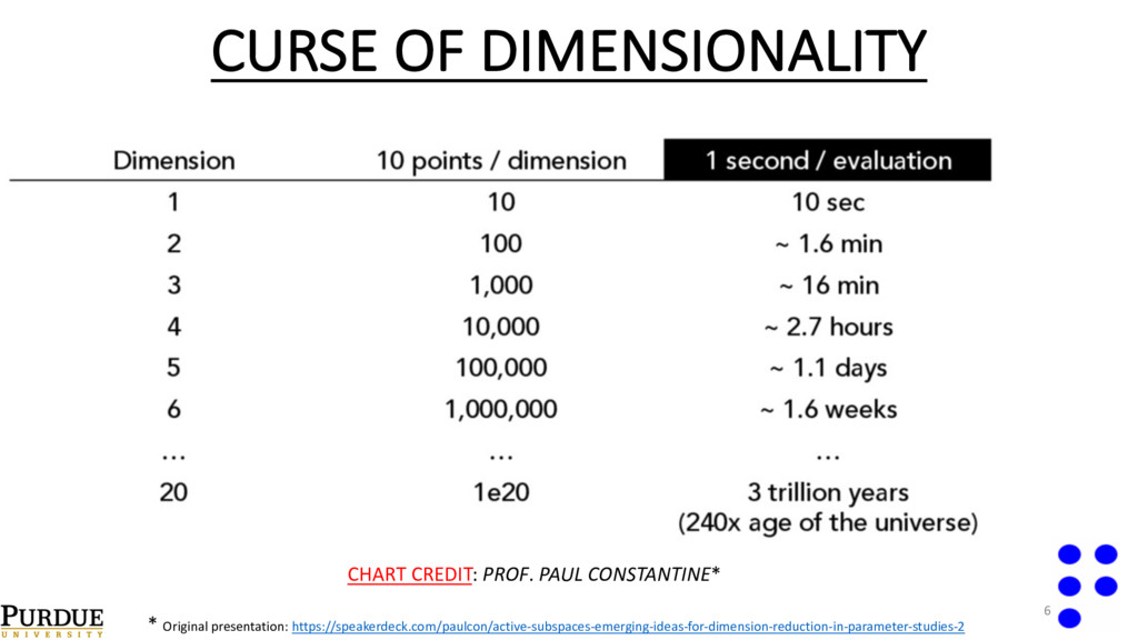
5. • The expectations have to be computed numerically. • Monte Carlo, although independent in the dimensionality, converges very slowly in the number of samples of f. • Idea -> Replace the simulator of f with a surrogate model. • Problem -> Curse of dimensionality. 5
6. CURSE OF DIMENSIONALITY CHART CREDIT: PROF. PAUL CONSTANTINE* * Original presentation: https://speakerdeck.com/paulcon/active-subspaces-emerging-ideas-for-dimension-reduction-in-parameter-studies-2 6
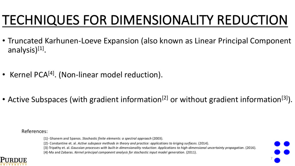
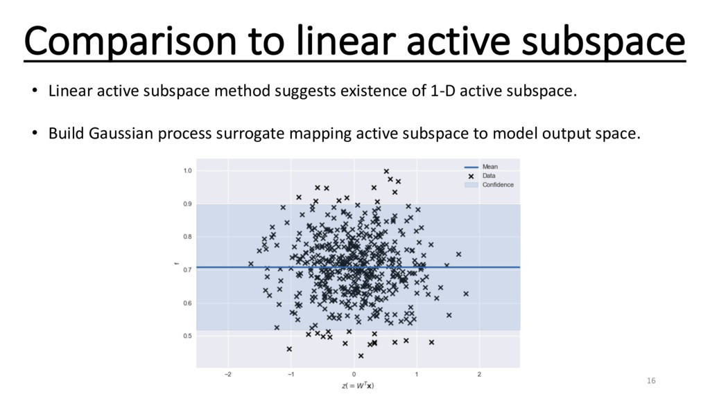
7. TECHNIQUES FOR DIMENSIONALITY REDUCTION • Truncated Karhunen-Loeve Expansion (also known as Linear Principal Component analysis)[1]. • Kernel PCA[4]. (Non-linear model reduction). • Active Subspaces (with gradient information[2] or without gradient information[3]). References: [1]- Ghanem and Spanos. Stochastic finite elements: a spectral approach (2003). [2]- Constantine et. al. Active subspace methods in theory and practice: applications to kriging surfaces. (2014). [3]-Tripathy et. al. Gaussian processes with built-in dimensionality reduction: Applications to high-dimensional uncertainty propagation. (2016). [4]-Ma and Zabaras. Kernel principal component analysis for stochastic input model generation. (2011). 7
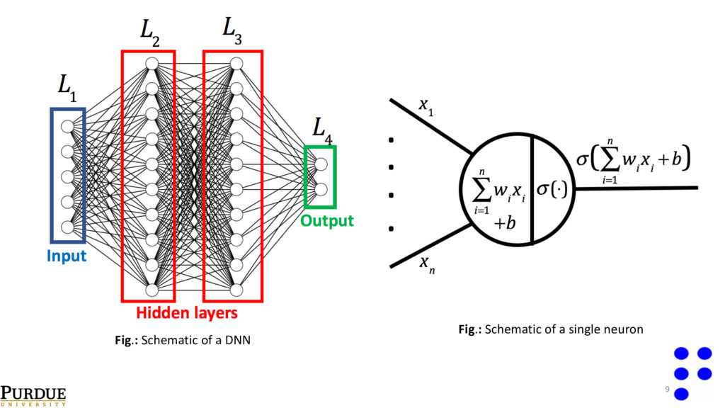
8. DEEP NEURAL NETWORKS o Universal function approximators[1]. o Layered representation of information[2]. o Linear regression can be thought of as a special case of DNNs (no hidden layers). o Tremendous success in recent times in applications such as image classification[2], autonomous driving[3]. o Availability of libraries such as tensorflow, keras, theano, PyTorch, caffe etc. References: [1]-Hornik . Approximation capabilities of multilayer feedforward networks. (1991). [2]-Krishevsky et al. Imagenet classification with deep convolutional neural networks. (2012). [3]-Chen et. al. Deepdriving: Learning affordance for direct perception in autonomous driving. (2015). 8
9. Fig.: Schematic of a DNN Fig.: Schematic of a single neuron 9
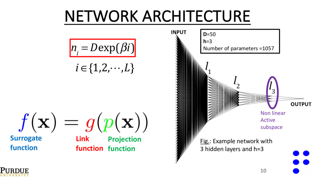
10. NETWORK ARCHITECTURE INPUT OUTPUT l 1 l 2 Fig.: Example network with 3 hidden layers and h=3 10 n i = Dexp(βi) i ∈{1,2,!,L} l 3 D=50 h=3 Number of parameters =1057 Projection function Surrogate function Link function Non linear Active subspace
11. OPTIMIZATION Likelihood model: Full Loss function: NEGATIVE LOG LIKELIHOOD REGULARIZER 11 L j (θ,λ,σ ;a j )= log(σ )+ 1 2σ 2 ( y j − F(a j ;θ))2 y|a,θ,σ ~ N (|F(a,θ),σ 2) θ* ,σ * ,λ* = argminL L = 1 N j=1 N ∑L j + λ l=1 L+1 ∑oW l o 2
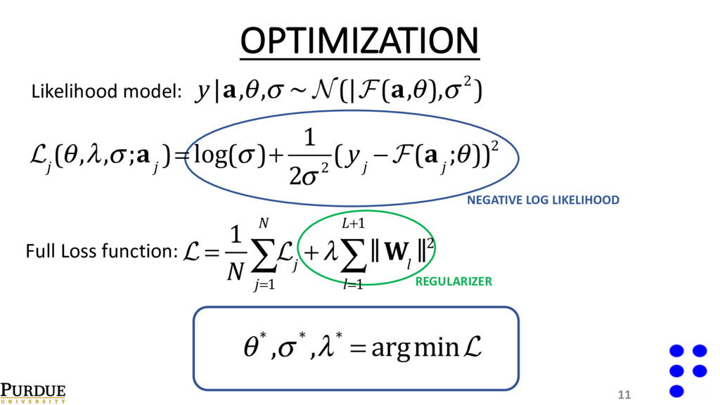
12. o Backpropagation[2] to compute gradients. o Use mini-batch size of 32. o Initial stepsize set to 1x10-4 . o Drop stepsize by factor of 1/10 every 15k iterations. o Train for 45k iterations. o Moment decay rate: . β 1 = 0.9,β 2 = 0.999 θ t =θ t−1 −α m t v t +ε 12 ADAptive Moments (ADAM[1]) optimizer References: [1]- Kingma and Ba. Adam: A method for stochastic optimization. (2014). [2]- Rummelhart and Yves, Backpropagation: theory, architectures, and applications. (1995).
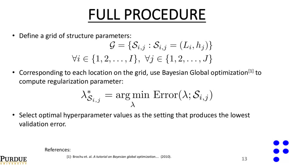
13. FULL PROCEDURE 13 • Define a grid of structure parameters: • Corresponding to each location on the grid, use Bayesian Global optimization[1] to compute regularization parameter: • Select optimal hyperparameter values as the setting that produces the lowest validation error. References: [1]- Brochu et. al. A tutorial on Bayesian global optimization…. (2010).
14. SYNTHETIC EXAMPLE 14
15. Grid of structure parameters: Optimal network hyperparameter values : 15
16. Comparison to linear active subspace • Linear active subspace method suggests existence of 1-D active subspace. • Build Gaussian process surrogate mapping active subspace to model output space. 16
17. What about when we have data from multifidelity sources? 17
18. Fidelity f1 f2 f3 18
19. f2 f3 f1 fs Parameters shared by f1, f2, ….., fs Parameters shared by f2, ….., fs Parameters shared by f3, ….., fs Parameters only trained with fs 19
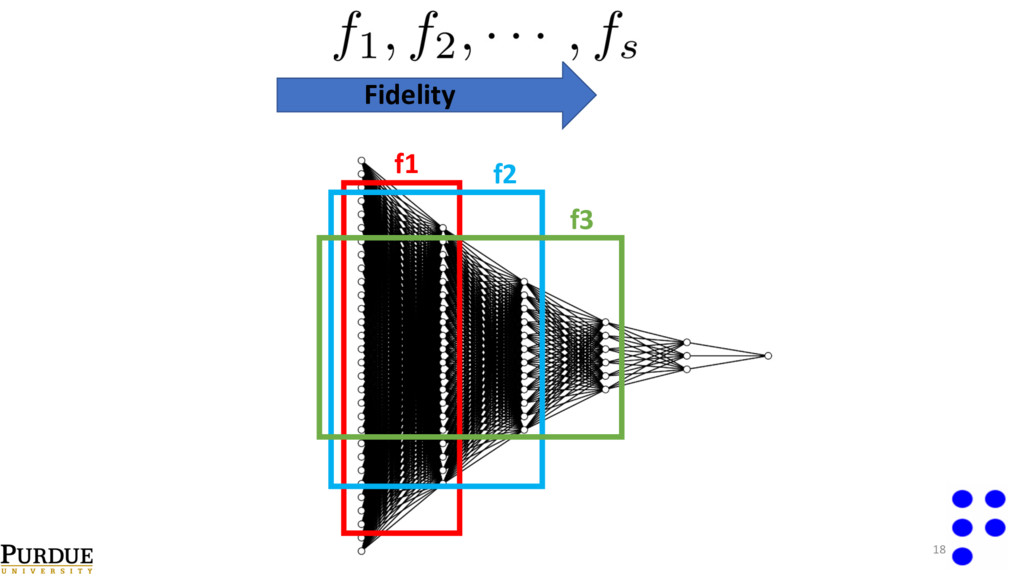
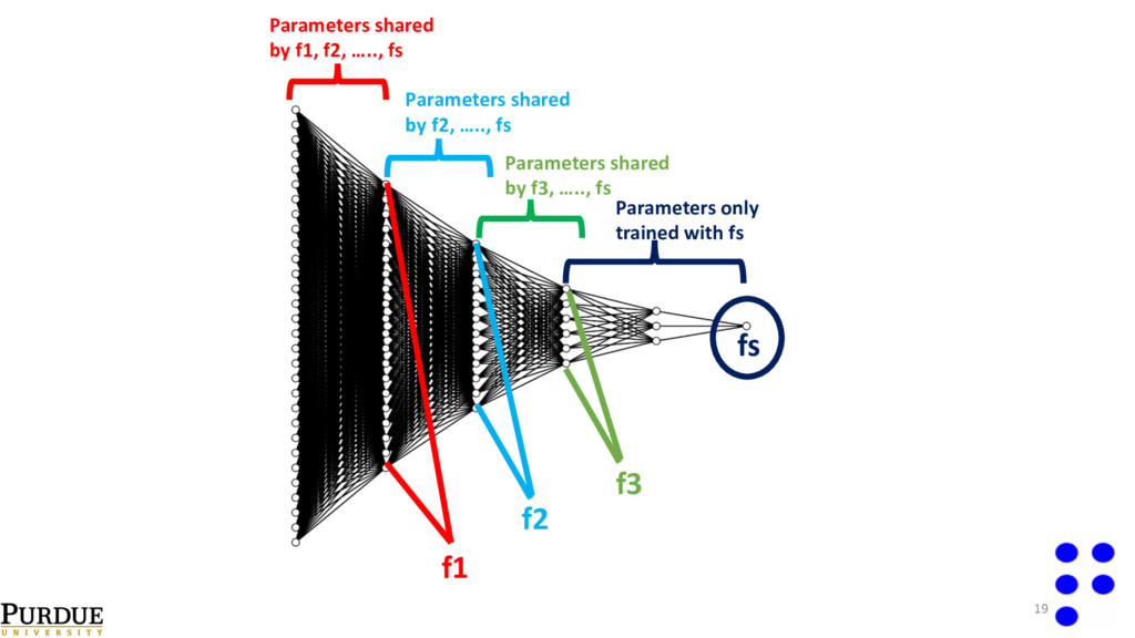
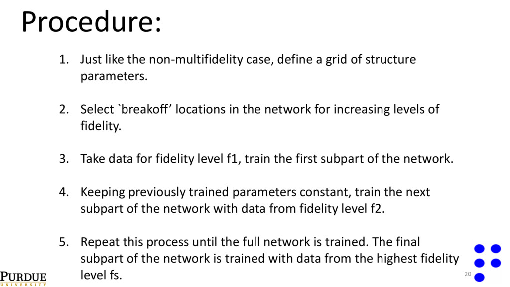
20. Procedure: 1. Just like the non-multifidelity case, define a grid of structure parameters. 2. Select `breakoff’ locations in the network for increasing levels of fidelity. 3. Take data for fidelity level f1, train the first subpart of the network. 4. Keeping previously trained parameters constant, train the next subpart of the network with data from fidelity level f2. 5. Repeat this process until the full network is trained. The final subpart of the network is trained with data from the highest fidelity level fs. 20
21. MULTIFIDELITY SYNTHETIC EXAMPLE High fidelity model: Low fidelity model: Dataset size: 21
22. Grid of structure parameters: Optimal network hyperparameter values : Low fidelity subnetwork break off point: 22
23. FUTURE WORK • Move to Bayesian setting – use advances in variational learning. • Explore convolutional networks for stochastic PDEs. • Treat breakoff points in multifidelity network as hyperparameters to be learned from data. THANK YOU ! 23