Bayesian joint models for multiple longitudinal biomarkers and time-to-event data: methods and software development

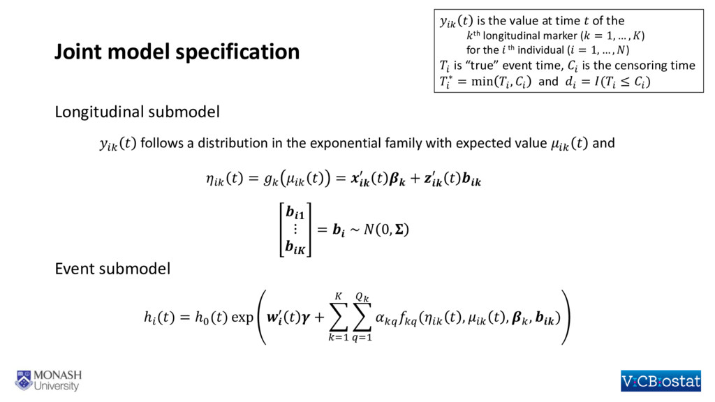
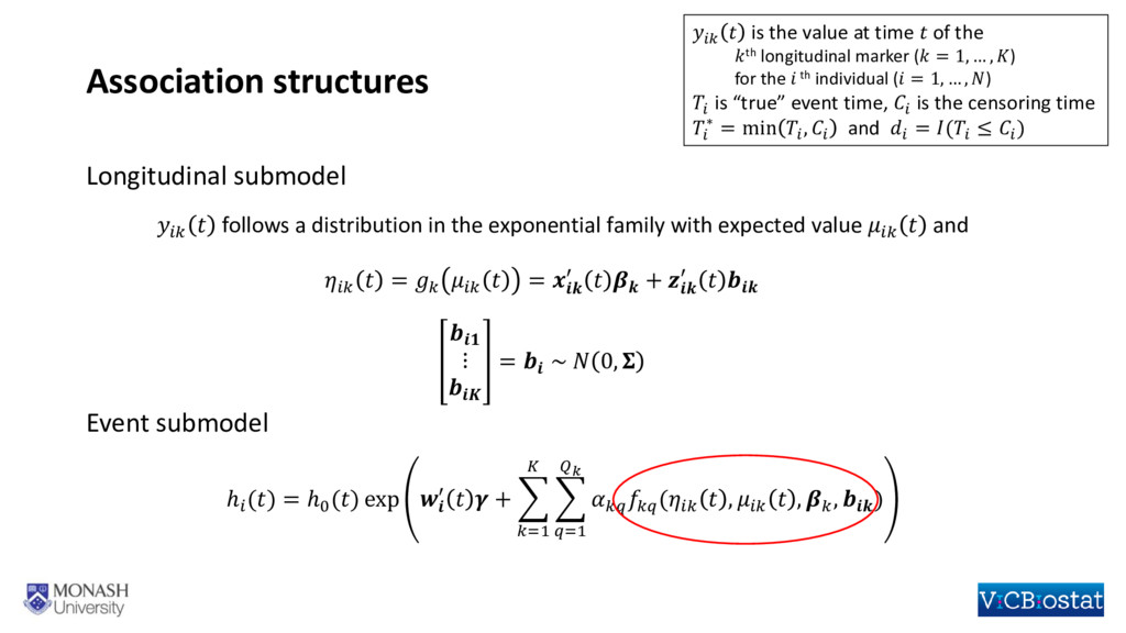
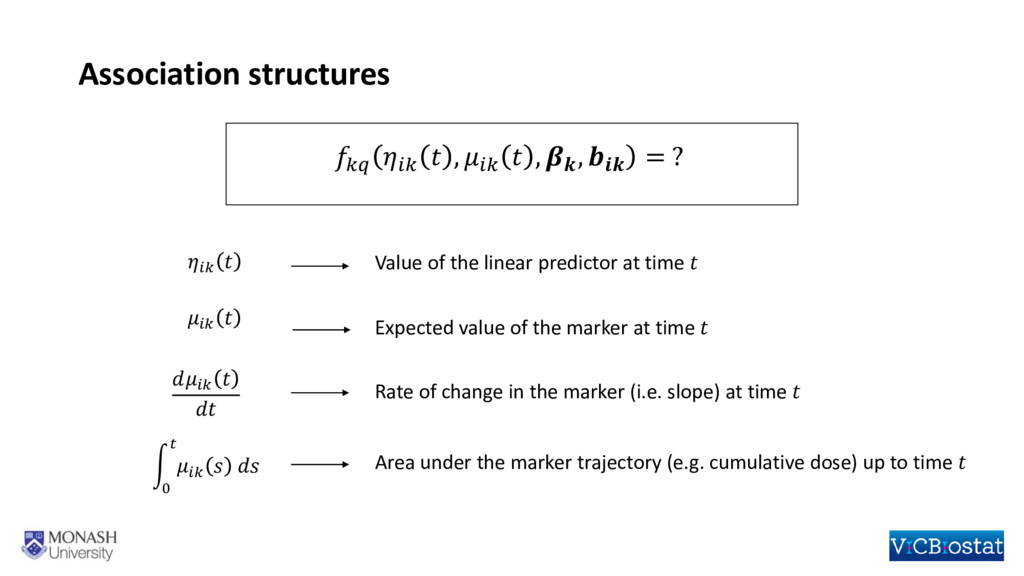
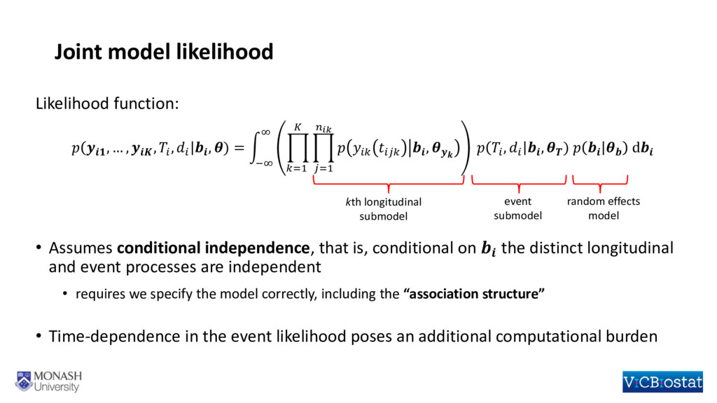
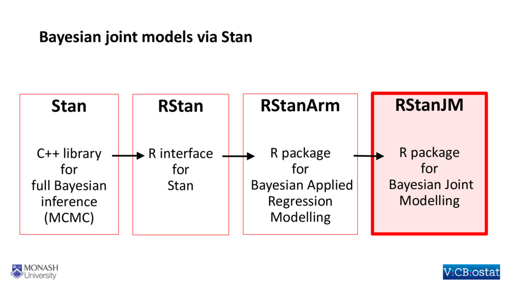
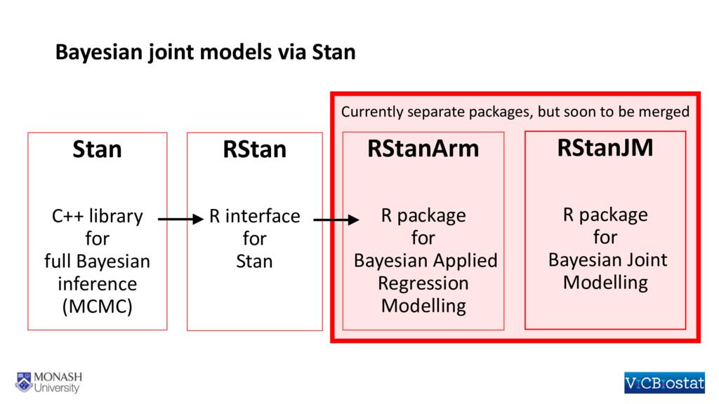
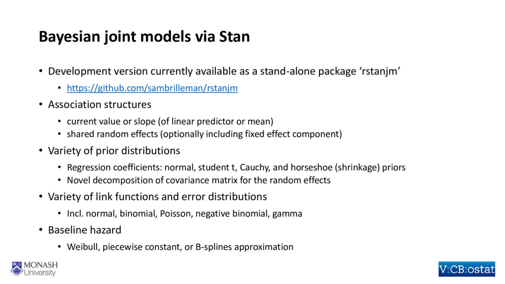
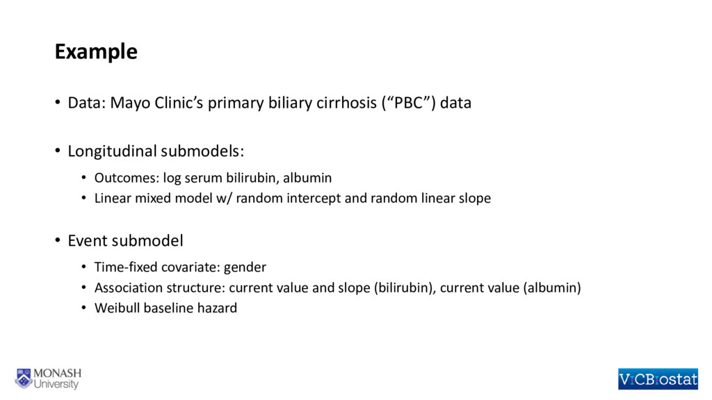
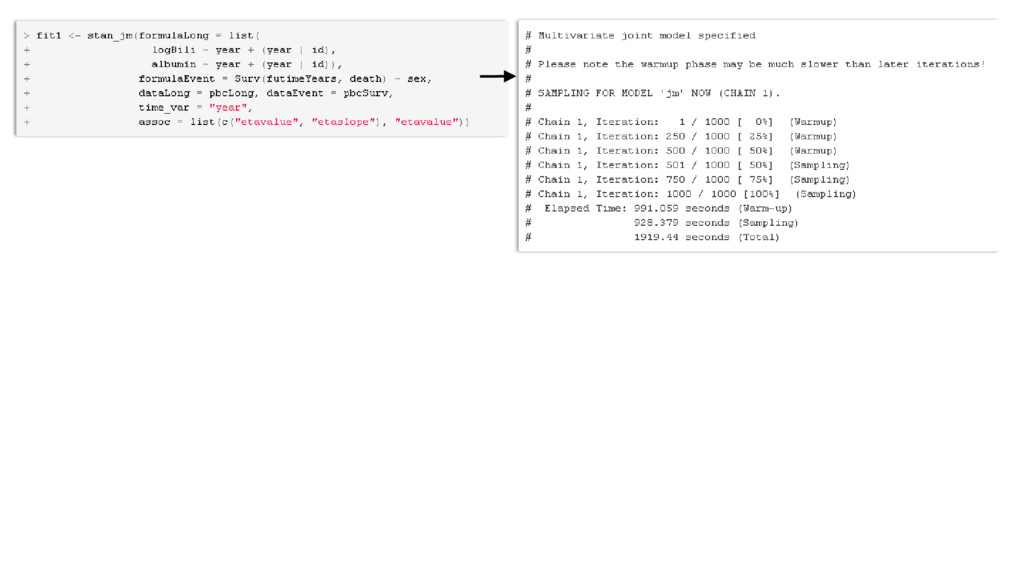
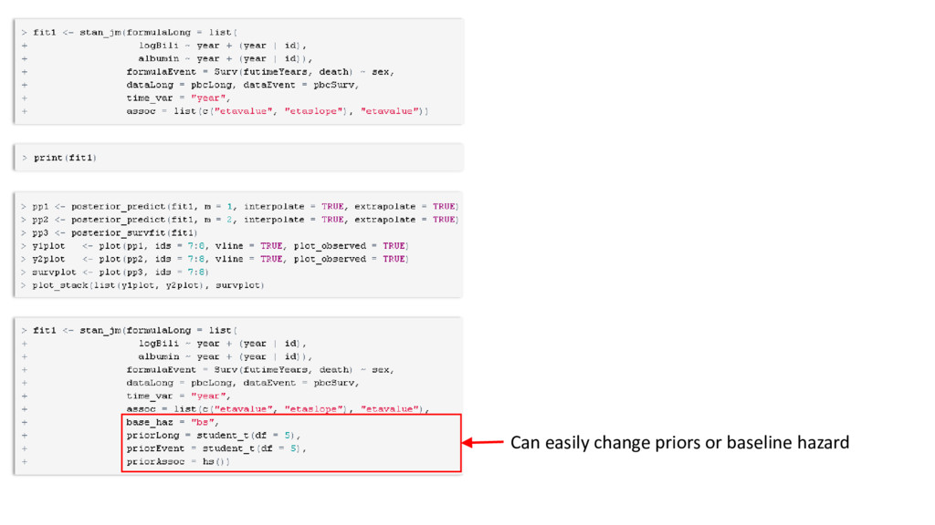
Methodological developments in the joint modelling of longitudinal and time-to-event data abound. Implementations of various versions of this methodology now enable researchers to fit joint models using standard statistical software packages. However, situations in which there are multiple longitudinal markers, or data clustered beyond the level of the individual, have not been widely considered and there is not yet readily available software for fitting joint models in either of these situations. In this talk I will outline the framework for fitting a shared parameter joint model for multiple longitudinal biomarkers and the time to an event. The longitudinal biomarkers are each modelled using a generalized linear mixed model which, through the use of cubic splines, can be extended to allow for flexible non-linear trajectories. The time-to-event is modelled through a parametric proportional hazards regression model. Dependence between multiple biomarkers is assumed to be captured through a shared multivariate normal distribution for the individual-level random effects, whilst the dependence between each biomarker and the time-to-event is based on shared random effects and can be parameterized in several ways. Estimation is under a Bayesian framework, which allows for the specification of a variety of prior distributions, such as shrinkage priors on regression coefficients, and the “LKJ” distribution for the correlation matrix on the individual-level random effects. Our approach easily extends to data that is clustered at levels beyond the individual, for example, when we have longitudinal and time-to-event data observed on patients within hospitals. I will briefly describe an R package rstanjm which facilitates fitting these models, by providing an interface to the software Stan. Stan (http://mc-stan.org) facilitates full Bayesian inference using an implementation of Hamiltonian Monte Carlo. I will demonstrate use of the R package through an example and discuss the potential benefits of using Stan for the underlying estimation.

Keywords: shared parameter model; joint model; Stan; Bayesian;

Transcript

1. Bayesian joint models for multiple longitudinal biomarkers and event-time data: methods and software development Sam Brilleman1,2, Michael J. Crowther3, Margarita Moreno-Betancur1,2,4, Rory Wolfe1,2 Australian Statistical Conference Canberra, Australia 5-9th December 2016 1 Monash University, Australia 2 Victorian Centre for Biostatistics (ViCBiostat) 3 University of Leicester, UK 4 Murdoch Childrens Research Institute, Australia
2. Background • The joint estimation of distinct regression models which, traditionally, we would have estimated separately • One or more longitudinal (mixed effects) models • each for a repeatedly measured clinical marker, e.g. systolic blood pressure • A survival or time-to-event (proportional hazards) model • for the time to an event, e.g. time-to-death, time-to-stroke What is joint modelling?
3. Background • We want to know whether the longitudinal marker is associated with the risk of the event • e.g. how is time-varying SBP associated with the risk of death? • can actually consider association between the event risk and any aspect of the longitudinal trajectory (e.g. slope) • can allow for measurement error in the marker • can allow for discrete-time measurement of the marker • And possibly other reasons… • e.g. dynamic predictions, separating out “direct” and “indirect” effects of treatment, adjusting for informative dropout Why use joint modelling?
4. Joint model specification follows a distribution in the exponential family with expected value and = = ′ + ′ ⋮ = ~ 0, Longitudinal submodel ℎ () = ℎ0 () exp ′ + ෍ =1 ෍ =1 ( , , , ) Event submodel is the value at time of the th longitudinal marker ( = 1, … , ) for the th individual ( = 1, … , ) is “true” event time, is the censoring time ∗ = min , and = ( ≤ )
5. Association structures follows a distribution in the exponential family with expected value and = = ′ + ′ ⋮ = ~ 0, Longitudinal submodel ℎ () = ℎ0 () exp ′ + ෍ =1 ෍ =1 ( , , , ) Event submodel is the value at time of the th longitudinal marker ( = 1, … , ) for the th individual ( = 1, … , ) is “true” event time, is the censoring time ∗ = min , and = ( ≤ )
6. Association structures , , , = ? න 0 Value of the linear predictor at time Expected value of the marker at time Rate of change in the marker (i.e. slope) at time Area under the marker trajectory (e.g. cumulative dose) up to time
7. Joint model likelihood Likelihood function: , … , , , , ) = න −∞ ∞ ෑ =1 ෑ =1 , , , ) d • Assumes conditional independence, that is, conditional on the distinct longitudinal and event processes are independent • requires we specify the model correctly, including the “association structure” • Time-dependence in the event likelihood poses an additional computational burden kth longitudinal submodel event submodel random effects model
8. Bayesian joint models via Stan RStanArm R package for Bayesian Applied Regression Modelling RStan R interface for Stan Stan C++ library for full Bayesian inference (MCMC) RStanJM R package for Bayesian Joint Modelling
9. Bayesian joint models via Stan RStanArm R package for Bayesian Applied Regression Modelling RStan R interface for Stan Stan C++ library for full Bayesian inference (MCMC) RStanJM R package for Bayesian Joint Modelling Currently separate packages, but soon to be merged
10. Bayesian joint models via Stan • Development version currently available as a stand-alone package ‘rstanjm’ • https://github.com/sambrilleman/rstanjm • Association structures • current value or slope (of linear predictor or mean) • shared random effects (optionally including fixed effect component) • Variety of prior distributions • Regression coefficients: normal, student t, Cauchy, and horseshoe (shrinkage) priors • Novel decomposition of covariance matrix for the random effects • Variety of link functions and error distributions • Incl. normal, binomial, Poisson, negative binomial, gamma • Baseline hazard • Weibull, piecewise constant, or B-splines approximation
11. Example • Data: Mayo Clinic’s primary biliary cirrhosis (“PBC”) data • Longitudinal submodels: • Outcomes: log serum bilirubin, albumin • Linear mixed model w/ random intercept and random linear slope • Event submodel • Time-fixed covariate: gender • Association structure: current value and slope (bilirubin), current value (albumin) • Weibull baseline hazard
17. Can easily change priors or baseline hazard
18. • My PhD supervisors: Rory Wolfe, Margarita Moreno-Betancur, Michael Crowther, John Carlin • My PhD funders: NHMRC and Victorian Centre for Biostatistics (ViCBiostat) • Staff from ViCBiostat  • Ben Goodrich and Jonah Gabry (authors of RStanArm) Thank you