Joint longitudinal and time-to-event models via Stan

Transcript

1. Joint longitudinal and time-to-event models via Stan Sam Brilleman1,2, Michael J. Crowther3, Margarita Moreno-Betancur2,4,5, Jacqueline Buros Novik6, Rory Wolfe1,2 StanCon 2018 Pacific Grove, California, USA 10-12th January 2018 1 Monash University, Melbourne, Australia 2 Victorian Centre for Biostatistics (ViCBiostat) 3 University of Leicester, Leicester, UK 4 Murdoch Childrens Research Institute, Melbourne, Australia 5 University of Melbourne, Melbourne, Australia 6 Icahn School of Medicine at Mount Sinai, New York, US
2. Outline • Context and background • Joint model formulation • Association structures • Software implementation via Stan / rstanarm • Example application 2
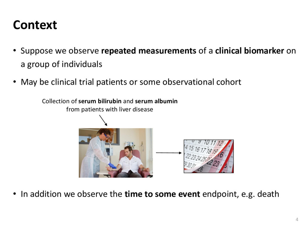
3. • Suppose we observe repeated measurements of a clinical biomarker on a group of individuals • May be clinical trial patients or some observational cohort Context 3 Collection of serum bilirubin and serum albumin from patients with liver disease
4. • Suppose we observe repeated measurements of a clinical biomarker on a group of individuals • May be clinical trial patients or some observational cohort • In addition we observe the time to some event endpoint, e.g. death Collection of serum bilirubin and serum albumin from patients with liver disease Context 4
5. Longitudinal and time-to-event data 5
6. What is “joint modelling” of longitudinal and time-to-event data? • Treats both the longitudinal biomarker(s) and the event as outcome data • Each outcome is modelled using a distinct regression submodel: • A (multivariate) mixed effects model for the longitudinal outcome(s) • A proportional hazards model for the time-to-event outcome • The regression submodels are linked through shared individual-specific parameters and estimated simultaneously under a joint likelihood function 6
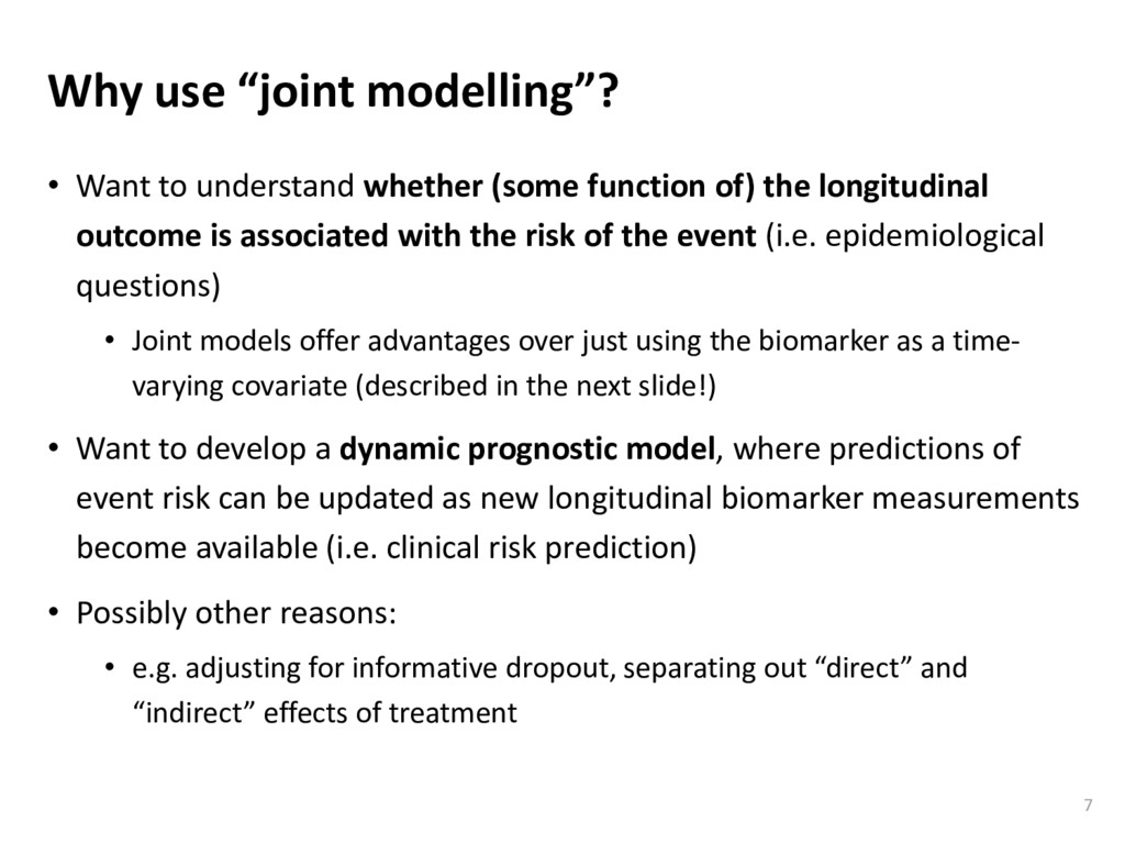
7. Why use “joint modelling”? 7 • Want to understand whether (some function of) the longitudinal outcome is associated with the risk of the event (i.e. epidemiological questions) • Joint models offer advantages over just using the biomarker as a time- varying covariate (described in the next slide!) • Want to develop a dynamic prognostic model, where predictions of event risk can be updated as new longitudinal biomarker measurements become available (i.e. clinical risk prediction) • Possibly other reasons: • e.g. adjusting for informative dropout, separating out “direct” and “indirect” effects of treatment
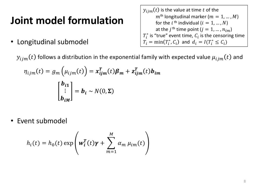
8. Joint model formulation • Longitudinal submodel • Event submodel 8 ℎ () = ℎ0 () exp + ෍ =1 () is the value at time of the th longitudinal marker ( = 1, … , ) for the th individual ( = 1, … , ) at the th time point ( = 1, … , ) ∗ is “true” event time, is the censoring time = min ∗, and = ( ∗ ≤ ) follows a distribution in the exponential family with expected value and = = + ⋮ = ~ 0,
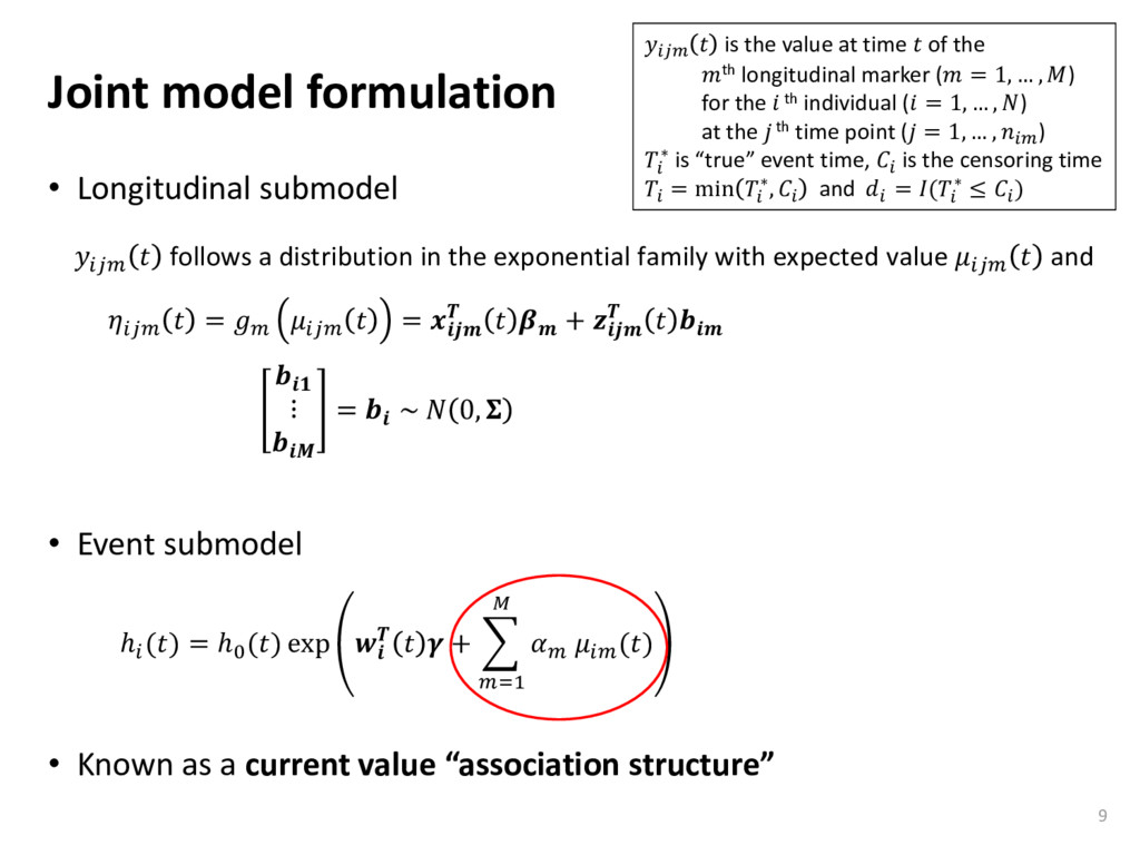
9. Joint model formulation • Longitudinal submodel • Event submodel • Known as a current value “association structure” 9 ℎ () = ℎ0 () exp + ෍ =1 () is the value at time of the th longitudinal marker ( = 1, … , ) for the th individual ( = 1, … , ) at the th time point ( = 1, … , ) ∗ is “true” event time, is the censoring time = min ∗, and = ( ∗ ≤ ) follows a distribution in the exponential family with expected value and = = + ⋮ = ~ 0,
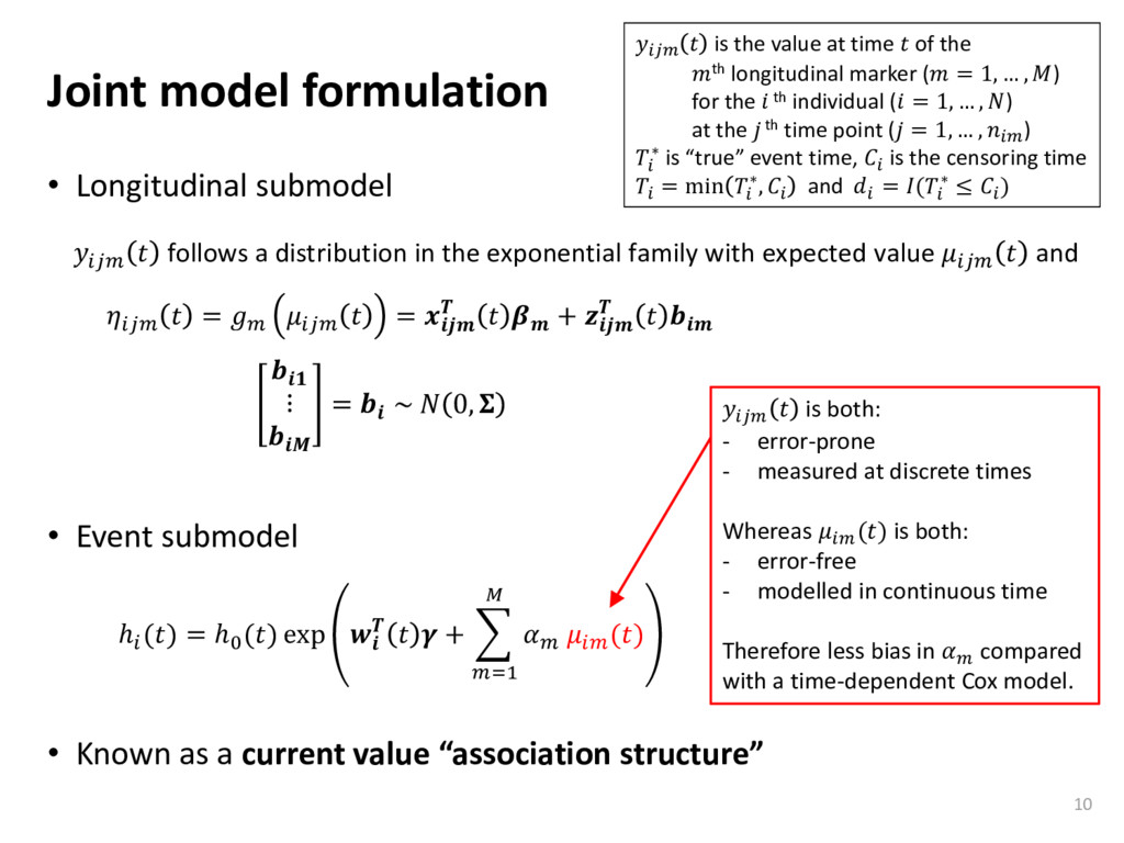
10. Joint model formulation • Longitudinal submodel • Event submodel • Known as a current value “association structure” 10 ℎ () = ℎ0 () exp + ෍ =1 () is the value at time of the th longitudinal marker ( = 1, … , ) for the th individual ( = 1, … , ) at the th time point ( = 1, … , ) ∗ is “true” event time, is the censoring time = min ∗, and = ( ∗ ≤ ) follows a distribution in the exponential family with expected value and = = + ⋮ = ~ 0, is both: - error-prone - measured at discrete times Whereas () is both: - error-free - modelled in continuous time Therefore less bias in compared with a time-dependent Cox model.
11. Association structures • A more general form for the event submodel is ℎ = ℎ0 exp + ෍ =1 ෍ =1 ( , ; ) 11
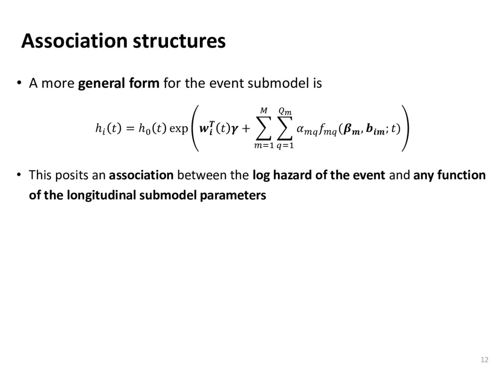
12. Association structures • A more general form for the event submodel is ℎ = ℎ0 exp + ෍ =1 ෍ =1 ( , ; ) • This posits an association between the log hazard of the event and any function of the longitudinal submodel parameters 12
13. Association structures • A more general form for the event submodel is ℎ = ℎ0 exp + ෍ =1 ෍ =1 ( , ; ) • This posits an association between the log hazard of the event and any function of the longitudinal submodel parameters; for example, defining (. ) as: 13 Linear predictor (or expected value of the biomarker) at time Rate of change in the linear predictor (or biomarker) at time Area under linear predictor (or biomarker trajectory), up to time න 0 − Lagged value (for some lag time )
14. Joint modelling software • An abundance of methodological developments in joint modelling • But not all methods have been translated into “user-friendly” software • Well established software for one longitudinal outcome • e.g. stjm (Stata); joineR, JM, JMbayes, frailtypack (R); JMFit (SAS) • Recent software developments for multiple longitudinal outcomes • R packages: rstanarm, joineRML, JMbayes, survtd • Each package has its strengths and limitations • e.g. (non-)normally distributed longitudinal outcomes, selected association structures, speed, etc. 14
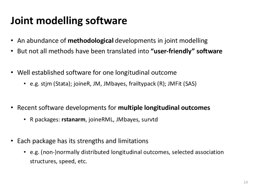
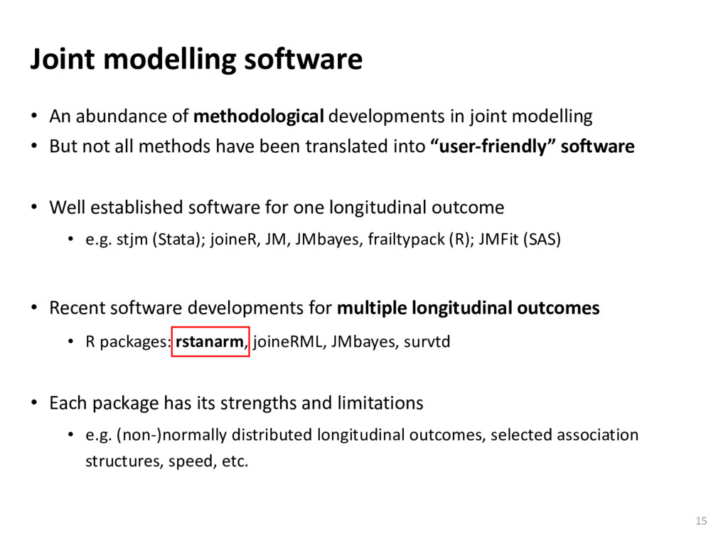
15. Joint modelling software • An abundance of methodological developments in joint modelling • But not all methods have been translated into “user-friendly” software • Well established software for one longitudinal outcome • e.g. stjm (Stata); joineR, JM, JMbayes, frailtypack (R); JMFit (SAS) • Recent software developments for multiple longitudinal outcomes • R packages: rstanarm, joineRML, JMbayes, survtd • Each package has its strengths and limitations • e.g. (non-)normally distributed longitudinal outcomes, selected association structures, speed, etc. 15
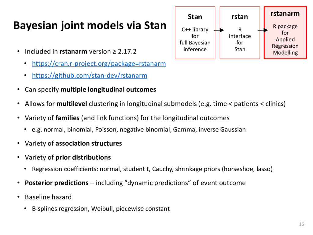
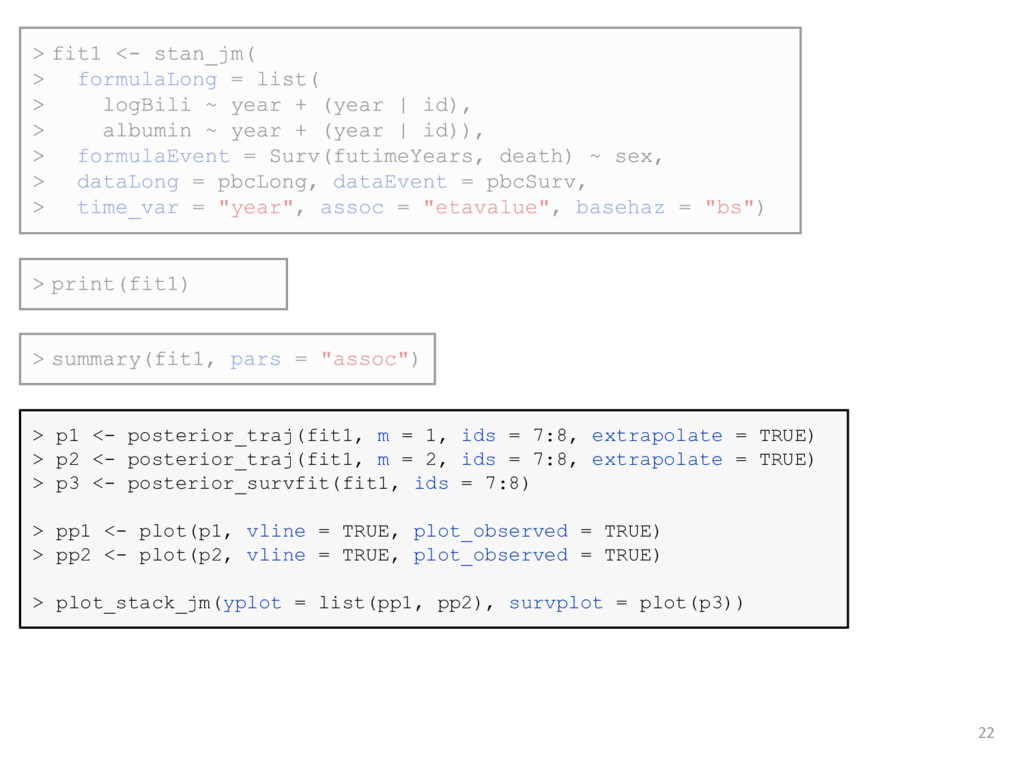
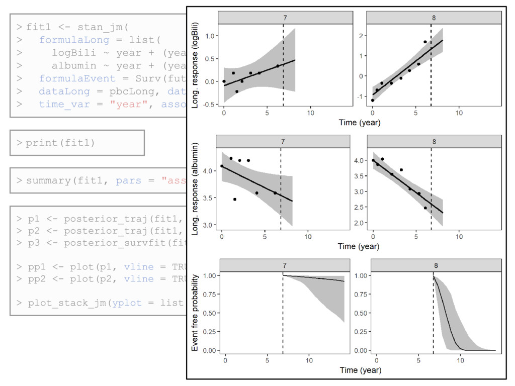
16. Bayesian joint models via Stan • Included in rstanarm version ≥ 2.17.2 • https://cran.r-project.org/package=rstanarm • https://github.com/stan-dev/rstanarm • Can specify multiple longitudinal outcomes • Allows for multilevel clustering in longitudinal submodels (e.g. time < patients < clinics) • Variety of families (and link functions) for the longitudinal outcomes • e.g. normal, binomial, Poisson, negative binomial, Gamma, inverse Gaussian • Variety of association structures • Variety of prior distributions • Regression coefficients: normal, student t, Cauchy, shrinkage priors (horseshoe, lasso) • Posterior predictions – including “dynamic predictions” of event outcome • Baseline hazard • B-splines regression, Weibull, piecewise constant rstan R interface for Stan Stan C++ library for full Bayesian inference rstanarm R package for Applied Regression Modelling 16
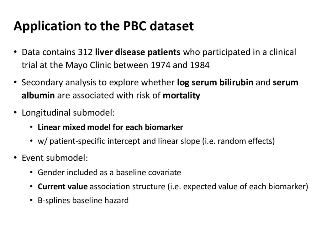
17. Application to the PBC dataset • Data contains 312 liver disease patients who participated in a clinical trial at the Mayo Clinic between 1974 and 1984 • Secondary analysis to explore whether log serum bilirubin and serum albumin are associated with risk of mortality • Longitudinal submodel: • Linear mixed model for each biomarker • w/ patient-specific intercept and linear slope (i.e. random effects) • Event submodel: • Gender included as a baseline covariate • Current value association structure (i.e. expected value of each biomarker) • B-splines baseline hazard
18. 18 ˃ fit1 <- stan_jm( ˃ formulaLong = list( ˃ logBili ~ year + (year | id), ˃ albumin ~ year + (year | id)), ˃ formulaEvent = Surv(futimeYears, death) ~ sex, ˃ dataLong = pbcLong, dataEvent = pbcSurv, ˃ time_var = "year", assoc = "etavalue", basehaz = "bs")
19. 19 ˃ print(fit1) # stan_jm # formula (Long1): logBili ~ year + (year | id) # family (Long1): gaussian [identity] # formula (Long2): albumin ~ year + (year | id) # family (Long2): gaussian [identity] # formula (Event): Surv(futimeYears, death) ~ sex # baseline hazard: bs # assoc: etavalue (Long1), etavalue (Long2) # ------ # # Longitudinal submodel 1: logBili # Median MAD_SD # (Intercept) 0.678 0.192 # year 0.227 0.042 # sigma 0.354 0.017 # # Longitudinal submodel 2: albumin # Median MAD_SD # (Intercept) 3.520 0.082 # year -0.161 0.025 # sigma 0.290 0.014 # # Event submodel: # Median MAD_SD exp(Median) # (Intercept) 7.054 2.870 1157.757 # sexf -0.182 0.674 0.834 # Long1|etavalue 0.745 0.281 2.105 # Long2|etavalue -3.141 0.857 0.043 ... # Group-level error terms: # Groups Name Std.Dev. Corr # id Long1|(Intercept) 1.2425 # Long1|year 0.1937 0.50 # Long2|(Intercept) 0.5029 -0.64 -0.51 # Long2|year 0.1022 -0.59 -0.81 0.47
20. 20 # stan_jm # formula (Long1): logBili ~ year + (year | id) # family (Long1): gaussian [identity] # formula (Long2): albumin ~ year + (year | id) # family (Long2): gaussian [identity] # formula (Event): Surv(futimeYears, death) ~ sex # baseline hazard: bs # assoc: etavalue (Long1), etavalue (Long2) # ------ # # Longitudinal submodel 1: logBili # Median MAD_SD # (Intercept) 0.678 0.192 # year 0.227 0.042 # sigma 0.354 0.017 # # Longitudinal submodel 2: albumin # Median MAD_SD # (Intercept) 3.520 0.082 # year -0.161 0.025 # sigma 0.290 0.014 # # Event submodel: # Median MAD_SD exp(Median) # (Intercept) 7.054 2.870 1157.757 # sexf -0.182 0.674 0.834 # Long1|etavalue 0.745 0.281 2.105 # Long2|etavalue -3.141 0.857 0.043 ... # Group-level error terms: # Groups Name Std.Dev. Corr # id Long1|(Intercept) 1.2425 # Long1|year 0.1937 0.50 # Long2|(Intercept) 0.5029 -0.64 -0.51 # Long2|year 0.1022 -0.59 -0.81 0.47 A one unit increase in log serum bilirubin is associated with an estimated 2.1-fold increase in the hazard of death
21. 21 ˃ summary(fit1, pars = "assoc") # Model Info: # # function: stan_jm # formula (Long1): logBili ~ year + (year | id) # family (Long1): gaussian [identity] # formula (Long2): albumin ~ year + (year | id) # family (Long2): gaussian [identity] # formula (Event): Surv(futimeYears, death) ~ sex # baseline hazard: bs # assoc: etavalue (Long1), etavalue (Lo # algorithm: sampling # priors: see help('prior_summary') # sample: 4000 (posterior sample size) # num obs: 304 (Long1), 304 (Long2) # num subjects: 40 # num events: 29 (72.5%) # groups: id (40) # runtime: 2.9 mins # # Estimates: # mean sd 2.5% 97.5% # Assoc|Long1|etavalue 0.748 0.281 0.204 1.302 # Assoc|Long2|etavalue -3.204 0.903 -5.121 -1.566 # # Diagnostics: # mcse Rhat n_eff # Assoc|Long1|etavalue 0.004 1.000 4000 # Assoc|Long2|etavalue 0.018 1.001 2452
22. 22 > p1 <- posterior_traj(fit1, m = 1, ids = 7:8, extrapolate = TRUE) > p2 <- posterior_traj(fit1, m = 2, ids = 7:8, extrapolate = TRUE) > p3 <- posterior_survfit(fit1, ids = 7:8) > pp1 <- plot(p1, vline = TRUE, plot_observed = TRUE) > pp2 <- plot(p2, vline = TRUE, plot_observed = TRUE) > plot_stack_jm(yplot = list(pp1, pp2), survplot = plot(p3))
23. 23 23
24. • StanCon committee and sponsor for support via the Student Scholarship • Eric Novik and Daniel Lee at Generable, for both academic support and financial support to get me here!  • Ben Goodrich and Jonah Gabry (maintainers of rstanarm) • Collaborators on motivating projects: Nidal Al-Huniti, James Dunyak and Robert Fox at AstraZeneca; Serigne Lo at Melanoma Institute Australia • My PhD supervisors: Rory Wolfe, Margarita Moreno-Betancur, Michael Crowther • My PhD funders: Australian National Health and Medical Research Council (NHMRC) and Victorian Centre for Biostatistics (ViCBiostat) • http://mc-stan.org/users/interfaces/rstanarm.html • https://github.com/stan-dev/rstanarm Acknowledgements References