simsurv: A Package for Simulating Simple or Complex Survival Data

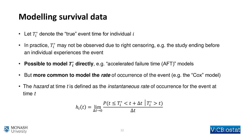
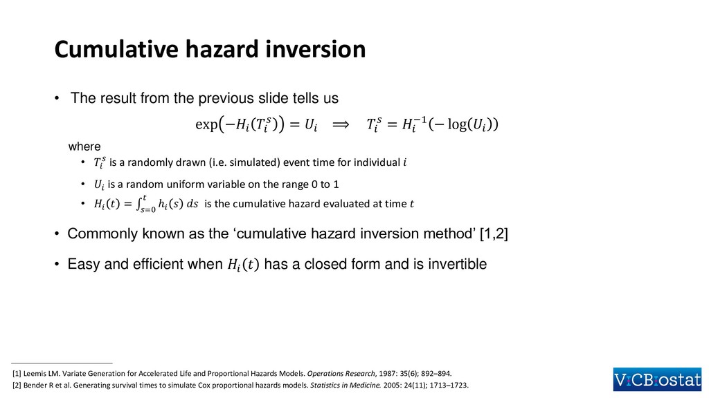
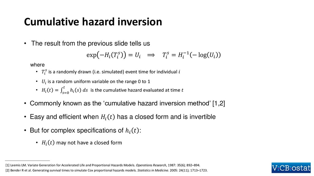
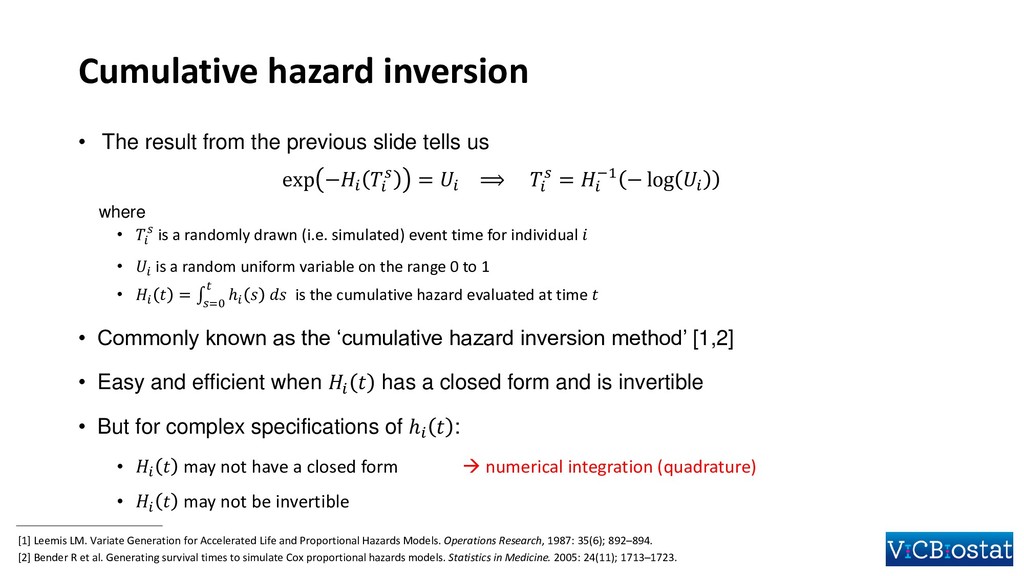
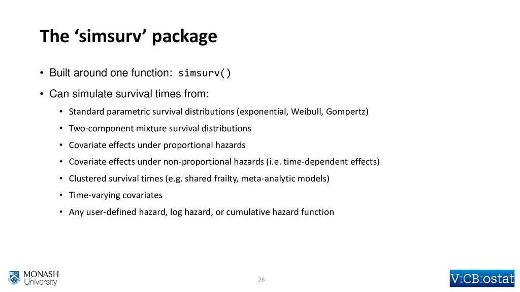
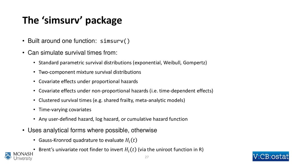
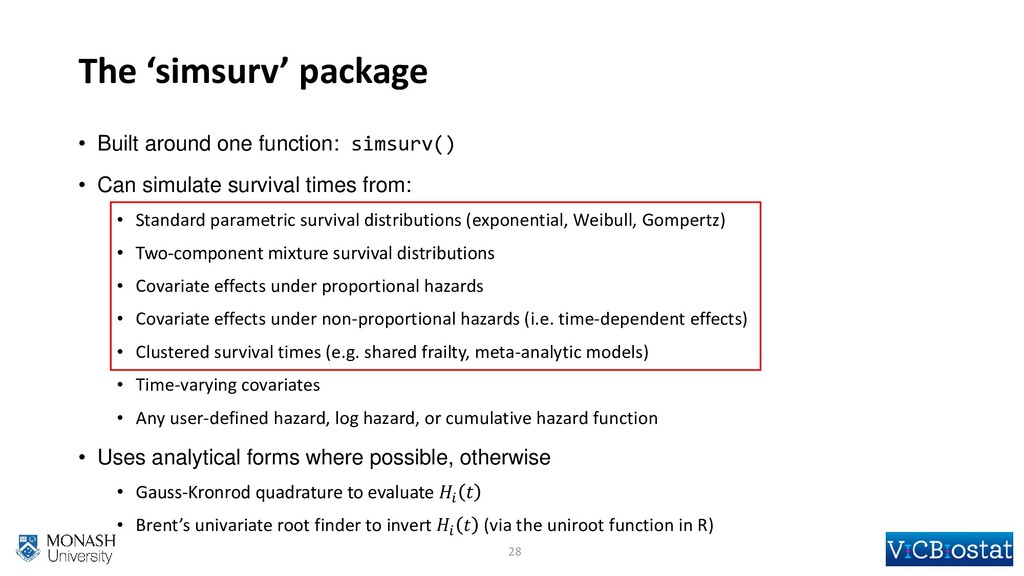
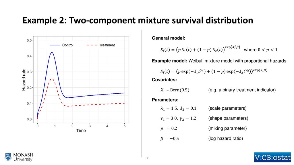
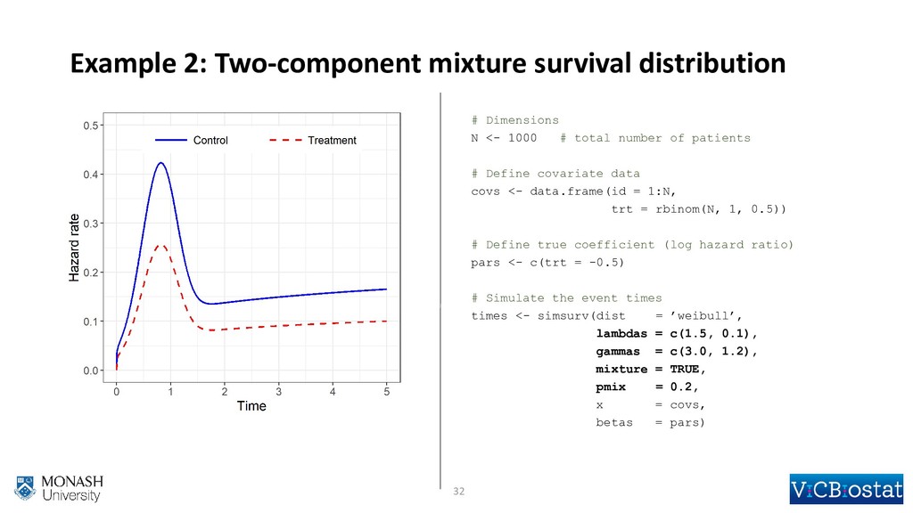
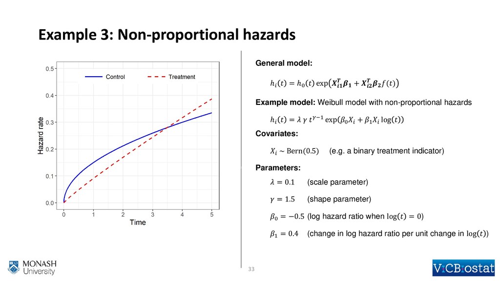
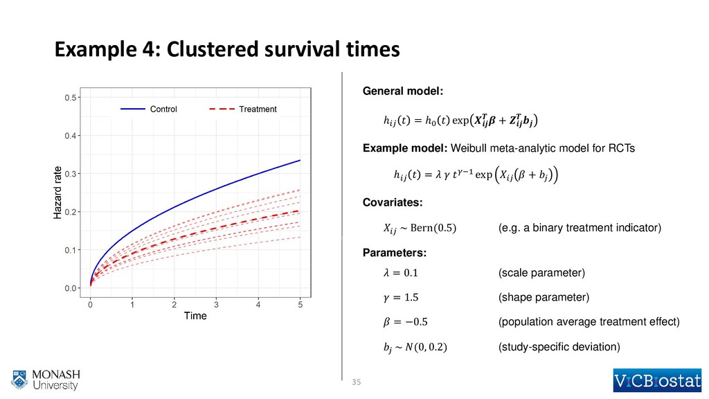
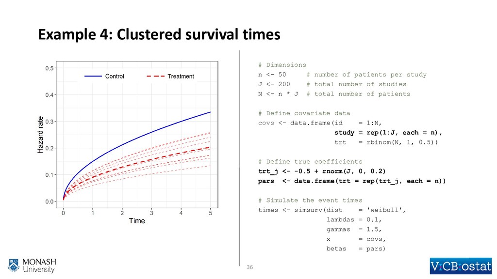
The simsurv package allows users to simulate simple or complex survival data. Survival data refers to a variable corresponding to the time from a defined baseline until occurrence of an event of interest. Depending on the field, the analysis of survival data can be known as survival, duration, reliability, or event history analysis. It has been common to make simplifying parametric assumptions when simulating survival data, e.g. assuming survival times follow an exponential or Weibull distribution. However, such assumptions are unrealistic in many settings. The simsurv package provides additional flexibility by allowing users to simulate survival times from 2-component mixture distributions or a user-defined hazard function. The mixture distributions allow for a variety of flexible baseline hazard functions. Moreover, a user-defined hazard function can provide even greater flexibility since the cumulative hazard does not require a closed-form solution. This means it is possible to simulate survival times under complex statistical models such as those for joint longitudinal-survival data. The package is modelled on the survsim package in Stata (Crowther and Lambert, 2012, Stata J).

Transcript

1. simsurv: A Package for
   Simulating Simple or Complex Survival Data
   Sam Brilleman1,2, Rory Wolfe1,2, Margarita Moreno-Betancur2,3,4, Michael J. Crowther5
   useR! Conference 2018
   Brisbane, Australia
   10-13th July 2018
   1 Monash University, Melbourne, Australia
   2 Victorian Centre for Biostatistics (ViCBiostat)
   3 Murdoch Children’s Research Institute, Melbourne, Australia
   4 University of Melbourne, Melbourne, Australia
   5 University of Leicester, Leicester, UK
   

   View Slide

2. Outline
   • Background to survival analysis
   • A general method for simulating event times
   • Examples of using the ‘simsurv’ package
   • Summary
   2
   

   View Slide

3. What is survival analysis?
   • The analysis of a variable that corresponds to the time from a defined baseline (e.g.
   diagnosis of a disease) until occurrence of an event of interest (e.g. heart failure).
   3
   

   View Slide

4. What is survival analysis?
   • The analysis of a variable that corresponds to the time from a defined baseline (e.g.
   diagnosis of a disease) until occurrence of an event of interest (e.g. heart failure).
   • Also known as:
   • Time-to-event analysis
   • Duration analysis (economics)
   • Reliability analysis (engineering)
   • Event history analysis (sociology)
   4
   

   View Slide

5. What is survival analysis?
   • The analysis of a variable that corresponds to the time from a defined baseline (e.g.
   diagnosis of a disease) until occurrence of an event of interest (e.g. heart failure).
   • Also known as:
   • Time-to-event analysis
   • Duration analysis (economics)
   • Reliability analysis (engineering)
   • Event history analysis (sociology)
   • The context for this talk will be health research
   • Each observational unit will be an “individual” (e.g. a patient)
   5
   

   View Slide

6. Why simulate survival data?
   • To evaluate the performance of new or existing statistical methods for survival analysis
   6
   

   View Slide

7. Why simulate survival data?
   • To evaluate the performance of new or existing statistical methods for survival analysis
   • To calculate statistical power, e.g. in planning clinical trials
   7
   

   View Slide

8. Why simulate survival data?
   • To evaluate the performance of new or existing statistical methods for survival analysis
   • To calculate statistical power, e.g. in planning clinical trials
   • To calculate uncertainty in model predictions, e.g. transition probabilities in multistate models
   8
   

   View Slide

9. Why simulate survival data?
   • To evaluate the performance of new or existing statistical methods for survival analysis
   • To calculate statistical power, e.g. in planning clinical trials
   • To calculate uncertainty in model predictions, e.g. transition probabilities in multistate models
   • …others?
   9
   

   View Slide

10. Modelling survival data
    • Let
    ∗ denote the “true” event time for individual
    • In practice,
    ∗ may not be observed due to right censoring, e.g. the study ending before
    an individual experiences the event
    10
    

    View Slide

11. Modelling survival data
    • Let
    ∗ denote the “true” event time for individual
    • In practice,
    ∗ may not be observed due to right censoring, e.g. the study ending before
    an individual experiences the event
    • Possible to model
    ∗ directly, e.g. “accelerated failure time (AFT)” models
    11
    

    View Slide

12. • Let
    ∗ denote the “true” event time for individual
    • In practice,
    ∗ may not be observed due to right censoring, e.g. the study ending before
    an individual experiences the event
    • Possible to model
    ∗ directly, e.g. “accelerated failure time (AFT)” models
    • But more common to model the rate of occurrence of the event (e.g. the “Cox” model)
    • The hazard at time t is defined as the instantaneous rate of occurrence for the event at
    time t
    ℎ
    = lim
    Δ→0
    ( ≤
    ∗ < + Δ │
    ∗ > )
    Δ
    Modelling survival data
    12
    

    View Slide

13. The hazard, cumulative hazard & survival
    • Hazard (for individual ): ℎ
    
    • Cumulative hazard:
    = ׬
    =0
    
    ℎ
    
    • Survival probability:
    =
    ∗ > = exp −
    
    13
    

    View Slide

14. The hazard, cumulative hazard & survival
    • Hazard (for individual ): ℎ
    
    • Cumulative hazard:
    = ׬
    =0
    
    ℎ
    
    • Survival probability:
    =
    ∗ > = exp −
    
    14
    This is the complement of the CDF for the distribution of event times
    

    View Slide

15. The hazard, cumulative hazard & survival
    • Hazard (for individual ): ℎ
    
    • Cumulative hazard:
    = ׬
    =0
    
    ℎ
    
    • Survival probability:
    =
    ∗ > = exp −
    
    • The “probability integral transformation” tells us 1 −
    = , where
    . is the CDF of
    a continuous random variable , and is a uniform random variable on the range 0 to 1
    15
    This is the complement of the CDF for the distribution of event times
    

    View Slide

16. Cumulative hazard inversion
    • The result from the previous slide tells us
    exp −
    
    =
    ⟹
    =
    −1 − log
    where
    •
    is a randomly drawn (i.e. simulated) event time for individual
    •
    is a random uniform variable on the range 0 to 1
    •
    = ׬
    =0
    
    ℎ
    is the cumulative hazard evaluated at time
    16
    

    View Slide

17. Cumulative hazard inversion
    • The result from the previous slide tells us
    exp −
    
    =
    ⟹
    =
    −1 − log
    where
    •
    is a randomly drawn (i.e. simulated) event time for individual
    •
    is a random uniform variable on the range 0 to 1
    •
    = ׬
    =0
    
    ℎ
    is the cumulative hazard evaluated at time
    • Commonly known as the ‘cumulative hazard inversion method’ [1,2]
    • Easy and efficient when
    has a closed form and is invertible
    [1] Leemis LM. Variate Generation for Accelerated Life and Proportional Hazards Models. Operations Research, 1987: 35(6); 892–894.
    [2] Bender R et al. Generating survival times to simulate Cox proportional hazards models. Statistics in Medicine. 2005: 24(11); 1713–1723.
    

    View Slide

18. Cumulative hazard inversion
    • The result from the previous slide tells us
    exp −
    
    =
    ⟹
    =
    −1 − log
    where
    •
    is a randomly drawn (i.e. simulated) event time for individual
    •
    is a random uniform variable on the range 0 to 1
    •
    = ׬
    =0
    
    ℎ
    is the cumulative hazard evaluated at time
    • Commonly known as the ‘cumulative hazard inversion method’ [1,2]
    • Easy and efficient when
    has a closed form and is invertible
    • But for complex specifications of ℎ
    :
    [1] Leemis LM. Variate Generation for Accelerated Life and Proportional Hazards Models. Operations Research, 1987: 35(6); 892–894.
    [2] Bender R et al. Generating survival times to simulate Cox proportional hazards models. Statistics in Medicine. 2005: 24(11); 1713–1723.
    

    View Slide

19. Cumulative hazard inversion
    • The result from the previous slide tells us
    exp −
    
    =
    ⟹
    =
    −1 − log
    where
    •
    is a randomly drawn (i.e. simulated) event time for individual
    •
    is a random uniform variable on the range 0 to 1
    •
    = ׬
    =0
    
    ℎ
    is the cumulative hazard evaluated at time
    • Commonly known as the ‘cumulative hazard inversion method’ [1,2]
    • Easy and efficient when
    has a closed form and is invertible
    • But for complex specifications of ℎ
    :
    •
    may not have a closed form
    [1] Leemis LM. Variate Generation for Accelerated Life and Proportional Hazards Models. Operations Research, 1987: 35(6); 892–894.
    [2] Bender R et al. Generating survival times to simulate Cox proportional hazards models. Statistics in Medicine. 2005: 24(11); 1713–1723.
    

    View Slide

20. Cumulative hazard inversion
    • The result from the previous slide tells us
    exp −
    
    =
    ⟹
    =
    −1 − log
    where
    •
    is a randomly drawn (i.e. simulated) event time for individual
    •
    is a random uniform variable on the range 0 to 1
    •
    = ׬
    =0
    
    ℎ
    is the cumulative hazard evaluated at time
    • Commonly known as the ‘cumulative hazard inversion method’ [1,2]
    • Easy and efficient when
    has a closed form and is invertible
    • But for complex specifications of ℎ
    :
    •
    may not have a closed form
    •
    may not be invertible
    [1] Leemis LM. Variate Generation for Accelerated Life and Proportional Hazards Models. Operations Research, 1987: 35(6); 892–894.
    [2] Bender R et al. Generating survival times to simulate Cox proportional hazards models. Statistics in Medicine. 2005: 24(11); 1713–1723.
    

    View Slide

21. Cumulative hazard inversion
    • The result from the previous slide tells us
    exp −
    
    =
    ⟹
    =
    −1 − log
    where
    •
    is a randomly drawn (i.e. simulated) event time for individual
    •
    is a random uniform variable on the range 0 to 1
    •
    = ׬
    =0
    
    ℎ
    is the cumulative hazard evaluated at time
    • Commonly known as the ‘cumulative hazard inversion method’ [1,2]
    • Easy and efficient when
    has a closed form and is invertible
    • But for complex specifications of ℎ
    :
    •
    may not have a closed form  numerical integration (quadrature)
    •
    may not be invertible
    [1] Leemis LM. Variate Generation for Accelerated Life and Proportional Hazards Models. Operations Research, 1987: 35(6); 892–894.
    [2] Bender R et al. Generating survival times to simulate Cox proportional hazards models. Statistics in Medicine. 2005: 24(11); 1713–1723.
    

    View Slide

22. [1] Leemis LM. Variate Generation for Accelerated Life and Proportional Hazards Models. Operations Research, 1987: 35(6); 892–894.
    [2] Bender R et al. Generating survival times to simulate Cox proportional hazards models. Statistics in Medicine. 2005: 24(11); 1713–1723.
    Cumulative hazard inversion
    • The result from the previous slide tells us
    exp −
    
    =
    ⟹
    =
    −1 − log
    where
    •
    is a randomly drawn (i.e. simulated) event time for individual
    •
    is a random uniform variable on the range 0 to 1
    •
    = ׬
    =0
    
    ℎ
    is the cumulative hazard evaluated at time
    • Commonly known as the ‘cumulative hazard inversion method’ [1,2]
    • Easy and efficient when
    has a closed form and is invertible
    • But for complex specifications of ℎ
    :
    •
    may not have a closed form  numerical integration (quadrature)
    •
    may not be invertible  iterative univariate root finding
    

    View Slide

23. [3] Crowther MJ, Lambert PC. Simulating Biologically Plausible Complex Survival Data. Statistics in Medicine, 2013: 32(23); 4118–4134.
    [4] Crowther MJ, Lambert PC. Simulating Complex Survival Data. The Stata Journal, 2012: 12(4); 674–687.
    [5] Brilleman S. (2018) simsurv: Simulate Survival Data. R package version 0.2.2. https://CRAN.R-project.org/package=simsurv
    • Crowther and Lambert [3] describe an algorithm as follows
    A general algorithm for simulating event times
    Does
    () have a
    closed form
    expression?
    Can you solve for
    
    analytically?
    Apply the
    cumulative hazard
    inversion method
    Use numerical integration to
    evaluate
    (), and nest it
    within iterative root finding
    to solve for
    
    Use iterative root
    finding to solve
    for
    
    Yes Yes
    No
    No
    

    View Slide

24. [3] Crowther MJ, Lambert PC. Simulating Biologically Plausible Complex Survival Data. Statistics in Medicine, 2013: 32(23); 4118–4134.
    [4] Crowther MJ, Lambert PC. Simulating Complex Survival Data. The Stata Journal, 2012: 12(4); 674–687.
    [5] Brilleman S. (2018) simsurv: Simulate Survival Data. R package version 0.2.2. https://CRAN.R-project.org/package=simsurv
    A general algorithm for simulating event times
    • Crowther and Lambert [3] describe an algorithm as follows
    • This method was implemented in a Stata package [4]
    • Now also implemented in R as part of the ‘simsurv’ package [5]
    Does
    () have a
    closed form
    expression?
    Can you solve for
    
    analytically?
    Apply the
    cumulative hazard
    inversion method
    Use numerical integration to
    evaluate
    (), and nest it
    within iterative root finding
    to solve for
    
    Use iterative root
    finding to solve
    for
    
    Yes Yes
    No
    No
    

    View Slide

25. The ‘simsurv’ package
    • Built around one function: simsurv()
    25
    

    View Slide

26. The ‘simsurv’ package
    • Built around one function: simsurv()
    • Can simulate survival times from:
    • Standard parametric survival distributions (exponential, Weibull, Gompertz)
    • Two-component mixture survival distributions
    • Covariate effects under proportional hazards
    • Covariate effects under non-proportional hazards (i.e. time-dependent effects)
    • Clustered survival times (e.g. shared frailty, meta-analytic models)
    • Time-varying covariates
    • Any user-defined hazard, log hazard, or cumulative hazard function
    26
    

    View Slide

27. The ‘simsurv’ package
    • Built around one function: simsurv()
    • Can simulate survival times from:
    • Standard parametric survival distributions (exponential, Weibull, Gompertz)
    • Two-component mixture survival distributions
    • Covariate effects under proportional hazards
    • Covariate effects under non-proportional hazards (i.e. time-dependent effects)
    • Clustered survival times (e.g. shared frailty, meta-analytic models)
    • Time-varying covariates
    • Any user-defined hazard, log hazard, or cumulative hazard function
    • Uses analytical forms where possible, otherwise
    • Gauss-Kronrod quadrature to evaluate
    
    • Brent’s univariate root finder to invert
    (via the uniroot function in R)
    27
    

    View Slide

28. The ‘simsurv’ package
    • Built around one function: simsurv()
    • Can simulate survival times from:
    • Standard parametric survival distributions (exponential, Weibull, Gompertz)
    • Two-component mixture survival distributions
    • Covariate effects under proportional hazards
    • Covariate effects under non-proportional hazards (i.e. time-dependent effects)
    • Clustered survival times (e.g. shared frailty, meta-analytic models)
    • Time-varying covariates
    • Any user-defined hazard, log hazard, or cumulative hazard function
    • Uses analytical forms where possible, otherwise
    • Gauss-Kronrod quadrature to evaluate
    
    • Brent’s univariate root finder to invert
    (via the uniroot function in R)
    28
    

    View Slide

29. Example 1: Standard parametric proportional hazards model
    29
    General model:
    ℎ
    = ℎ0
    exp
    
    Example model: Weibull model with proportional hazards
    ℎ
    = −1 exp
    
    Covariates:
    
    ~ Bern(0.5) (e.g. a binary treatment indicator)
    Parameters:
    = 0.1 (scale parameter)
    = 1.5 (shape parameter)
    = −0.5 (log hazard ratio)
    

    View Slide

30. Example 1: Standard parametric proportional hazards model
    30
    # Dimensions
    N <- 1000 # total number of patients
    # Define covariate data
    covs <- data.frame(id = 1:N,
    trt = rbinom(N, 1, 0.5))
    # Define true coefficient (log hazard ratio)
    pars <- c(trt = -0.5)
    # Simulate the event times
    times <- simsurv(dist = ’weibull’,
    lambdas = 0.1,
    gammas = 1.5,
    x = covs,
    betas = pars)
    

    View Slide

31. Example 2: Two-component mixture survival distribution
    31
    General model:
    
    = 1
    + 1 − 2
    exp
    
    where 0 < < 1
    Example model: Weibull mixture model with proportional hazards
    
    = exp −1
    1 + 1 − exp −2
    2 exp
    Covariates:
    
    ~ Bern(0.5) (e.g. a binary treatment indicator)
    Parameters:
    1
    = 1.5, 2
    = 0.1 (scale parameters)
    1
    = 3.0, 2
    = 1.2 (shape parameters)
    = 0.2 (mixing parameter)
    = −0.5 (log hazard ratio)
    

    View Slide

32. Example 2: Two-component mixture survival distribution
    32
    # Dimensions
    N <- 1000 # total number of patients
    # Define covariate data
    covs <- data.frame(id = 1:N,
    trt = rbinom(N, 1, 0.5))
    # Define true coefficient (log hazard ratio)
    pars <- c(trt = -0.5)
    # Simulate the event times
    times <- simsurv(dist = ’weibull’,
    lambdas = c(1.5, 0.1),
    gammas = c(3.0, 1.2),
    mixture = TRUE,
    pmix = 0.2,
    x = covs,
    betas = pars)
    

    View Slide

33. 33
    General model:
    ℎ
    = ℎ0
    exp
    
    +
    
    ()
    Example model: Weibull model with non-proportional hazards
    ℎ
    = −1 exp 0
    
    + 1
    
    log
    Covariates:
    
    ~ Bern(0.5) (e.g. a binary treatment indicator)
    Parameters:
    = 0.1 (scale parameter)
    = 1.5 (shape parameter)
    0
    = −0.5 (log hazard ratio when log = 0)
    1
    = 0.4 (change in log hazard ratio per unit change in log )
    Example 3: Non-proportional hazards
    

    View Slide

34. 34
    Example 3: Non-proportional hazards
    # Dimensions
    N <- 1000 # total number of patients
    # Define covariate data
    covs <- data.frame(id = 1:N,
    trt = rbinom(N, 1, 0.5))
    # Define true coefficients
    pars <- c(trt = -0.5) # time-fixed coefficient
    pars_tde <- c(trt = 0.4) # time-varying coefficient
    # Simulate the event times
    times <- simsurv(dist = 'weibull',
    lambdas = 0.1,
    gammas = 1.5,
    x = covs,
    betas = pars,
    tde = pars_tde,
    tdefun = 'log')
    

    View Slide

35. 35
    Example 4: Clustered survival times
    General model:
    ℎ
    = ℎ0
    exp
    +
    
    Example model: Weibull meta-analytic model for RCTs
    ℎ
    = −1 exp
    +
    Covariates:
    
    ~ Bern(0.5) (e.g. a binary treatment indicator)
    Parameters:
    = 0.1 (scale parameter)
    = 1.5 (shape parameter)
    = −0.5 (population average treatment effect)
    
    ~ (0, 0.2) (study-specific deviation)
    

    View Slide

36. # Dimensions
    n <- 50 # number of patients per study
    J <- 200 # total number of studies
    N <- n * J # total number of patients
    # Define covariate data
    covs <- data.frame(id = 1:N,
    study = rep(1:J, each = n),
    trt = rbinom(N, 1, 0.5))
    # Define true coefficients
    trt_j <- -0.5 + rnorm(J, 0, 0.2)
    pars <- data.frame(trt = rep(trt_j, each = n))
    # Simulate the event times
    times <- simsurv(dist = 'weibull',
    lambdas = 0.1,
    gammas = 1.5,
    x = covs,
    betas = pars)
    36
    Example 4: Clustered survival times
    

    View Slide

37. Summary
    • The method only requires that we can specify the hazard for the data generating model
    37
    

    View Slide

38. Summary
    • The method only requires that we can specify the hazard for the data generating model
    • I showed examples for some common scenarios, for which ‘simsurv’ has convenient
    arguments the user can specify
    38
    

    View Slide

39. Summary
    • The method only requires that we can specify the hazard for the data generating model
    • I showed examples for some common scenarios, for which ‘simsurv’ has convenient
    arguments the user can specify
    • I did not demonstrate “user-defined” hazard functions, which can allow even more flexibility
    • e.g. time-varying covariates, joint longitudinal-survival models, Royston-Parmar models, etc
    39
    

    View Slide

40. Summary
    • The method only requires that we can specify the hazard for the data generating model
    • I showed examples for some common scenarios, for which ‘simsurv’ has convenient
    arguments the user can specify
    • I did not demonstrate “user-defined” hazard functions, which can allow even more flexibility
    • e.g. time-varying covariates, joint longitudinal-survival models, Royston-Parmar models, etc
    • Computation times are “relatively” fast, e.g.
    • 10,000 event times under a standard Weibull distribution (< 1 sec)
    • 10,000 event times under a user-defined hazard function (~10 sec)
    40
    

    View Slide

41. Summary
    • The method only requires that we can specify the hazard for the data generating model
    • I showed examples for some common scenarios, for which ‘simsurv’ has convenient
    arguments the user can specify
    • I did not demonstrate “user-defined” hazard functions, which can allow even more flexibility
    • e.g. time-varying covariates, joint longitudinal-survival models, Royston-Parmar models, etc
    • Computation times are “relatively” fast, e.g.
    • 10,000 event times under a standard Weibull distribution (< 1 sec)
    • 10,000 event times under a user-defined hazard function (~10 sec)
    • Future work: competing risks, vectorisation of ‘uniroot’
    41
    

    View Slide

42. Thank you!
    [1] Leemis LM. Variate Generation for Accelerated Life and Proportional Hazards Models. Operations Research, 1987: 35(6); 892–894.
    [2] Bender R et al. Generating survival times to simulate Cox proportional hazards models. Statistics in Medicine. 2005: 24(11); 1713–1723.
    [3] Crowther MJ, Lambert PC. Simulating Biologically Plausible Complex Survival Data. Statistics in Medicine, 2013: 32(23); 4118–4134.
    [4] Crowther MJ, Lambert PC. Simulating Complex Survival Data. The Stata Journal, 2012: 12(4); 674–687.
    [5] Brilleman S. (2018) simsurv: Simulate Survival Data. R package version 0.2.2. https://CRAN.R-project.org/package=simsurv
    42
    References
    Acknowledgements
    • My supervisors: Rory Wolfe, Margarita Moreno-Betancur, Michael J. Crowther
    • CRAN and useR volunteers!
    

    View Slide