Bayesian joint models for multiple longitudinal biomarkers and a time-to-event outcome: software development and a melanoma case study

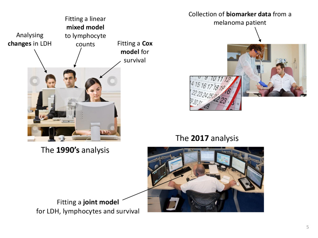
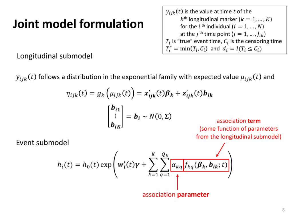
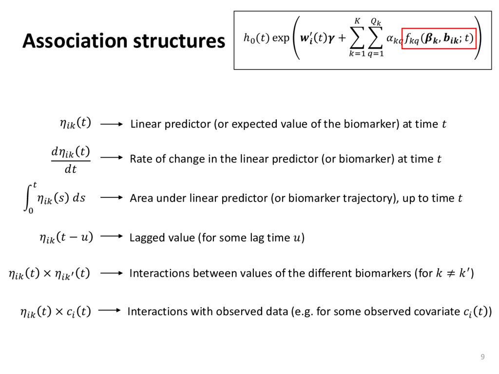
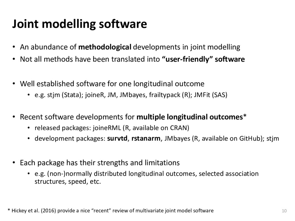
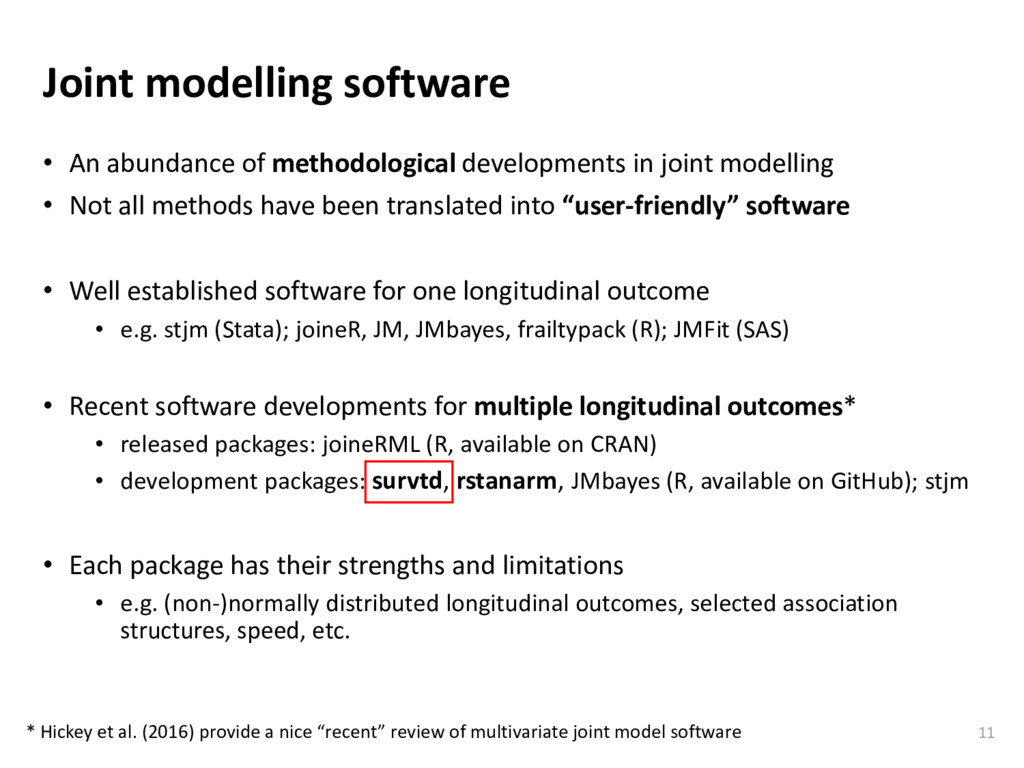
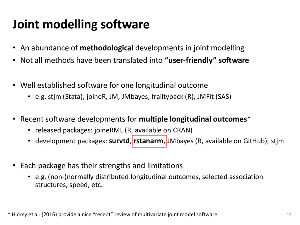
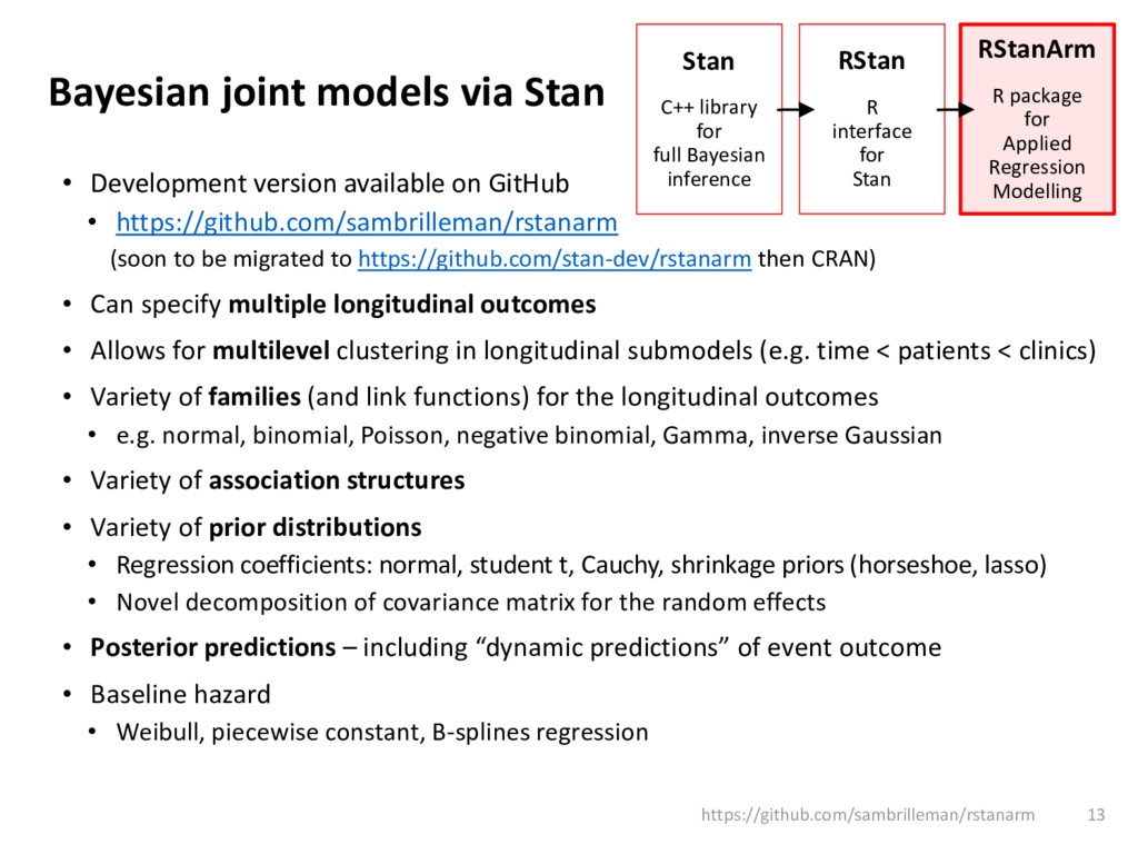
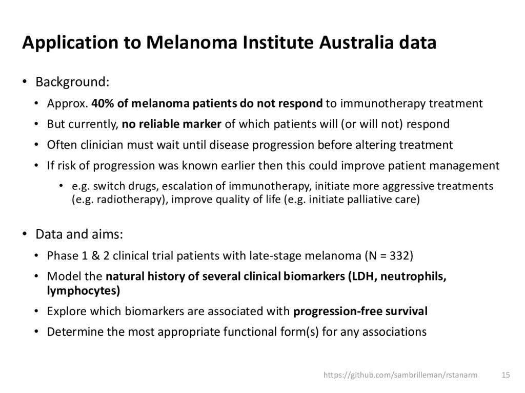
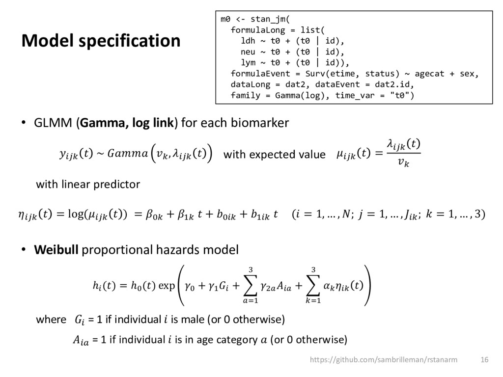
Methodological developments in the joint modelling of longitudinal and time-to-event data abound. Implementations of various versions of this methodology now enable researchers to fit joint models using standard statistical software packages. Yet the software options available to users remain limited in several respects. In particular, situations in which there are multiple longitudinal markers are not well accommodated. The modelling of longitudinal biomarker data in patients diagnosed with melanoma, and their association with the risk of clinical events such as death or disease progression, is one situation in which such extensions would prove useful. A framework for fitting a multivariate joint model can be specified as follows. The longitudinal biomarkers are each modelled using a generalized linear mixed model, whilst the time-to-event is modelled through a parametric proportional hazards regression model. Dependence between the multiple biomarkers within a subject is captured through shared subject-specific random effects following a multivariate normal distribution. Dependence between each biomarker and the time-to-event can be parameterised in a variety of ways. This project motivated the development of general purpose software that allows users to fit these multivariate joint models under a Bayesian approach, now implemented as part of the rstanarm R package. Using data from the Melanoma Institute Australia, I will demonstrate how these models can be used to provide insights into the relationships between patient-specific longitudinal trajectories for biomarkers such as LDH, neutrophils and lymphocyte counts, and the risk of either death or disease progression.

Keywords: shared parameter model; joint model; melanoma; Stan; Bayesian;

Transcript

1. Bayesian joint models for multiple longitudinal biomarkers and a time-to-event outcome: software development and a melanoma case study Sam Brilleman1,2, Michael J. Crowther3, Margarita Moreno-Betancur2,4,5, Serigne Lo6, Jacqueline Buros Novik7, Rory Wolfe1,2 38th Annual Conference of the International Society for Clinical Biostatistics Vigo, Spain 9-13th July 2017 1 Monash University, Melbourne, Australia 2 Victorian Centre for Biostatistics (ViCBiostat) 3 University of Leicester, Leicester, UK 4 Murdoch Childrens Research Institute, Melbourne, Australia 5 University of Melbourne, Melbourne, Australia 6 Melanoma Institute Australia, Sydney, Australia 7 Icahn School of Medicine at Mount Sinai, New York, US
2. Collection of biomarker data from a melanoma patient 2
3. Collection of biomarker data from a melanoma patient 3
4. Collection of biomarker data from a melanoma patient The 1990’s analysis Fitting a Cox model for survival Fitting a linear mixed model to lymphocyte counts Analysing changes in LDH 4
5. Collection of biomarker data from a melanoma patient The 1990’s analysis Fitting a Cox model for survival Fitting a linear mixed model to lymphocyte counts Analysing changes in LDH The 2017 analysis Fitting a joint model for LDH, lymphocytes and survival 5
6. Background • What is joint modelling? • The joint estimation of regression models which, traditionally, we would have estimated separately: • A (multivariate) longitudinal mixed model for a longitudinal outcome(s) • A time-to-event model for the time to an event of interest • The “sub”models are linked through shared (subject-specific) parameters • Why use it? • We want to understand how (some function of) the longitudinal outcome is associated with risk of the event • can allow for measurement error in the biomarker • can allow for discrete-time measurement of the biomarker • “Dynamic” predictions of the risk of the event • Separating out “direct” and “indirect” effects of treatment • Adjusting for informative dropout 6
7. Joint model formulation 7 ℎ () = ℎ0 () exp ′ + ෍ =1 ෍ =1 ( , ; ) Event submodel is the value at time of the th longitudinal marker ( = 1, … , ) for the th individual ( = 1, … , ) at the th time point ( = 1, … , ) is “true” event time, is the censoring time ∗ = min , and = ( ≤ ) follows a distribution in the exponential family with expected value and = = ′ + ′ ⋮ = ~ 0, Longitudinal submodel
8. Joint model formulation 8 ℎ () = ℎ0 () exp ′ + ෍ =1 ෍ =1 ( , ; ) Event submodel is the value at time of the th longitudinal marker ( = 1, … , ) for the th individual ( = 1, … , ) at the th time point ( = 1, … , ) is “true” event time, is the censoring time ∗ = min , and = ( ≤ ) follows a distribution in the exponential family with expected value and = = ′ + ′ ⋮ = ~ 0, Longitudinal submodel association parameter association term (some function of parameters from the longitudinal submodel)
9. Association structures 9 Linear predictor (or expected value of the biomarker) at time Rate of change in the linear predictor (or biomarker) at time Area under linear predictor (or biomarker trajectory), up to time න 0 ℎ0 () exp ′ + ෍ =1 ෍ =1 ( , ; ) − Lagged value (for some lag time ) × ′ Interactions between values of the different biomarkers (for ≠ ′) × Interactions with observed data (e.g. for some observed covariate )
10. Joint modelling software • An abundance of methodological developments in joint modelling • Not all methods have been translated into “user-friendly” software • Well established software for one longitudinal outcome • e.g. stjm (Stata); joineR, JM, JMbayes, frailtypack (R); JMFit (SAS) • Recent software developments for multiple longitudinal outcomes* • released packages: joineRML (R, available on CRAN) • development packages: survtd, rstanarm, JMbayes (R, available on GitHub); stjm • Each package has their strengths and limitations • e.g. (non-)normally distributed longitudinal outcomes, selected association structures, speed, etc. 10 * Hickey et al. (2016) provide a nice “recent” review of multivariate joint model software
11. Joint modelling software • An abundance of methodological developments in joint modelling • Not all methods have been translated into “user-friendly” software • Well established software for one longitudinal outcome • e.g. stjm (Stata); joineR, JM, JMbayes, frailtypack (R); JMFit (SAS) • Recent software developments for multiple longitudinal outcomes* • released packages: joineRML (R, available on CRAN) • development packages: survtd, rstanarm, JMbayes (R, available on GitHub); stjm • Each package has their strengths and limitations • e.g. (non-)normally distributed longitudinal outcomes, selected association structures, speed, etc. 11 * Hickey et al. (2016) provide a nice “recent” review of multivariate joint model software
12. Joint modelling software • An abundance of methodological developments in joint modelling • Not all methods have been translated into “user-friendly” software • Well established software for one longitudinal outcome • e.g. stjm (Stata); joineR, JM, JMbayes, frailtypack (R); JMFit (SAS) • Recent software developments for multiple longitudinal outcomes* • released packages: joineRML (R, available on CRAN) • development packages: survtd, rstanarm, JMbayes (R, available on GitHub); stjm • Each package has their strengths and limitations • e.g. (non-)normally distributed longitudinal outcomes, selected association structures, speed, etc. 12 * Hickey et al. (2016) provide a nice “recent” review of multivariate joint model software
13. Bayesian joint models via Stan • Development version available on GitHub • https://github.com/sambrilleman/rstanarm (soon to be migrated to https://github.com/stan-dev/rstanarm then CRAN) • Can specify multiple longitudinal outcomes • Allows for multilevel clustering in longitudinal submodels (e.g. time < patients < clinics) • Variety of families (and link functions) for the longitudinal outcomes • e.g. normal, binomial, Poisson, negative binomial, Gamma, inverse Gaussian • Variety of association structures • Variety of prior distributions • Regression coefficients: normal, student t, Cauchy, shrinkage priors (horseshoe, lasso) • Novel decomposition of covariance matrix for the random effects • Posterior predictions – including “dynamic predictions” of event outcome • Baseline hazard • Weibull, piecewise constant, B-splines regression RStan R interface for Stan Stan C++ library for full Bayesian inference RStanArm R package for Applied Regression Modelling https://github.com/sambrilleman/rstanarm 13
14. Bayesian joint models via Stan • Development version available on GitHub • https://github.com/sambrilleman/rstanarm (soon to be migrated to https://github.com/stan-dev/rstanarm then CRAN) • Can specify multiple longitudinal outcomes • Allows for multilevel clustering in longitudinal submodels (e.g. time < patients < clinics) • Variety of families (and link functions) for the longitudinal outcomes • e.g. normal, binomial, Poisson, negative binomial, Gamma, inverse Gaussian • Variety of association structures • Variety of prior distributions • Regression coefficients: normal, student t, Cauchy, shrinkage priors (horseshoe, lasso) • Novel decomposition of covariance matrix for the random effects • Posterior predictions – including “dynamic predictions” of event outcome • Baseline hazard • Weibull, piecewise constant, B-splines regression RStan R interface for Stan Stan C++ library for full Bayesian inference RStanArm R package for Applied Regression Modelling https://github.com/sambrilleman/rstanarm 14
15. Application to Melanoma Institute Australia data • Background: • Approx. 40% of melanoma patients do not respond to immunotherapy treatment • But currently, no reliable marker of which patients will (or will not) respond • Often clinician must wait until disease progression before altering treatment • If risk of progression was known earlier then this could improve patient management • e.g. switch drugs, escalation of immunotherapy, initiate more aggressive treatments (e.g. radiotherapy), improve quality of life (e.g. initiate palliative care) • Data and aims: • Phase 1 & 2 clinical trial patients with late-stage melanoma (N = 332) • Model the natural history of several clinical biomarkers (LDH, neutrophils, lymphocytes) • Explore which biomarkers are associated with progression-free survival • Determine the most appropriate functional form(s) for any associations https://github.com/sambrilleman/rstanarm 15
16. Model specification • GLMM (Gamma, log link) for each biomarker with linear predictor • Weibull proportional hazards model where = 1 if individual is male (or 0 otherwise) = 1 if individual is in age category (or 0 otherwise) https://github.com/sambrilleman/rstanarm 16 ℎ () = ℎ0 () exp 0 + 1 + ෍ =1 3 2 + ෍ =1 3 = log( ) = 0 + 1 + 0 + 1 ( = 1, … , ; = 1, … , ; = 1, … , 3) ~ , = with expected value m0 <- stan_jm( formulaLong = list( ldh ~ t0 + (t0 | id), neu ~ t0 + (t0 | id), lym ~ t0 + (t0 | id)), formulaEvent = Surv(etime, status) ~ agecat + sex, dataLong = dat2, dataEvent = dat2.id, family = Gamma(log), time_var = "t0")
17. Since a one unit increase in log(LDH) corresponds to an exp(1) = 2.7-fold increase in LDH, we can say that: “A 2.7-fold increase in mean LDH is associated with an estimated 1.6-fold increase in the hazard of death or disease progression” Hazard ratios (event submodel) Coefficient (log HR) Standard error (posterior SD) Hazard ratio Age category (years, ref: ≤50) 51 to 60 -0.166 0.274 0.847 61 to 70 0.113 0.267 1.120 71 and above 0.050 0.279 1.052 Gender (ref: Female) Male -0.110 0.211 0.896 Association parameters LDH (log value) 0.461 0.192 1.586 Neutrophils (log value) 2.287 0.454 9.845 Lymphocytes (log value) -0.472 0.286 0.624 https://github.com/sambrilleman/rstanarm 17
18. Posterior predictions (longitudinal) 18 pp_check(m0, m = 1) pp_check(m0, m = 2) pp_check(m0, m = 3) plot(posterior_traj(m0, ids = c(5,6,9))
19. Posterior predictions (event) 19 (0, 50] (50, 60] (60, 70] (70, 100] Age (in years) Cancer staging: presence of metastasis M1B M1C M0, M1A ps_check # overall standardised survival vs KM ids <- … # obtain IDs of individuals in risk group plot(posterior_survfit(m0, ids = ids, time = 0, standardise = TRUE))
20. Association structures allowing for effect modification • Interaction term between the (log) value of the biomarker and gender 20 • Interaction term between the (log) value of the biomarker and cancer stage/severity m1 <- update(m0, assoc = c(“etavalue”, “etavalue_data(~ gender)) m2 <- update(m0, assoc = c(“etavalue”, “etavalue_data(~ stage))
21. • Ben Goodrich and Jonah Gabry (maintainers of RStanArm) • ISCB (esp. Nadine Binder) for support via the Student Conference Award (StCA) • My PhD supervisors: Rory Wolfe, Margarita Moreno-Betancur, Michael Crowther • My PhD funders: NHMRC and Victorian Centre for Biostatistics (ViCBiostat) • Colleagues at Monash University and ViCBiostat • https://github.com/sambrilleman/rstanarm • http://mc-stan.org/users/interfaces/rstanarm.html • https://github.com/moreno-betancur/survtd • Moreno-Betancur M, Carlin JB, Brilleman SL, Tanamas S, Peeters A, Wolfe R. Survival analysis with time- dependent covariates subject to measurement error and missing data: Two-stage joint model using multiple imputation. 2016 (submitted). • Hickey GL, Philipson P, Jorgensen A, Kolamunnage-Dona R. Joint modelling of time-to-event and multivariate longitudinal outcomes: recent developments and issues. BMC Med Res Methodol. 2016; 16(1): 117. Acknowledgements References
24. Estimation Likelihood function: , … , , , , ) = න −∞ ∞ ෑ =1 ෑ =1 , , , ) d • Assumes conditional independence, that is, conditional on the distinct longitudinal and event processes are independent • requires we specify the model correctly, including the association structure • rstanarm uses a full Bayesian specification (i.e. includes priors) • Estimation via MCMC (Hamiltonian Monte Carlo) or, less preferably, variational Bayes https://github.com/sambrilleman/rstanarm 24 kth longitudinal submodel event submodel random effects model