Joint longitudinal and time-to-event models for multilevel hierarchical data

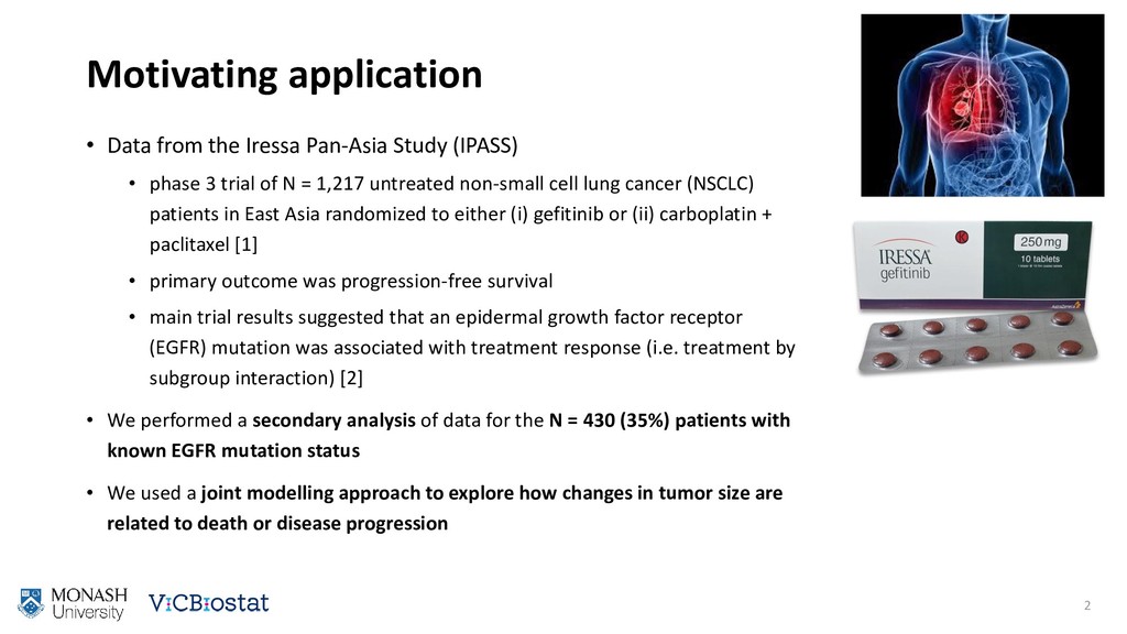
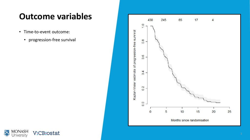
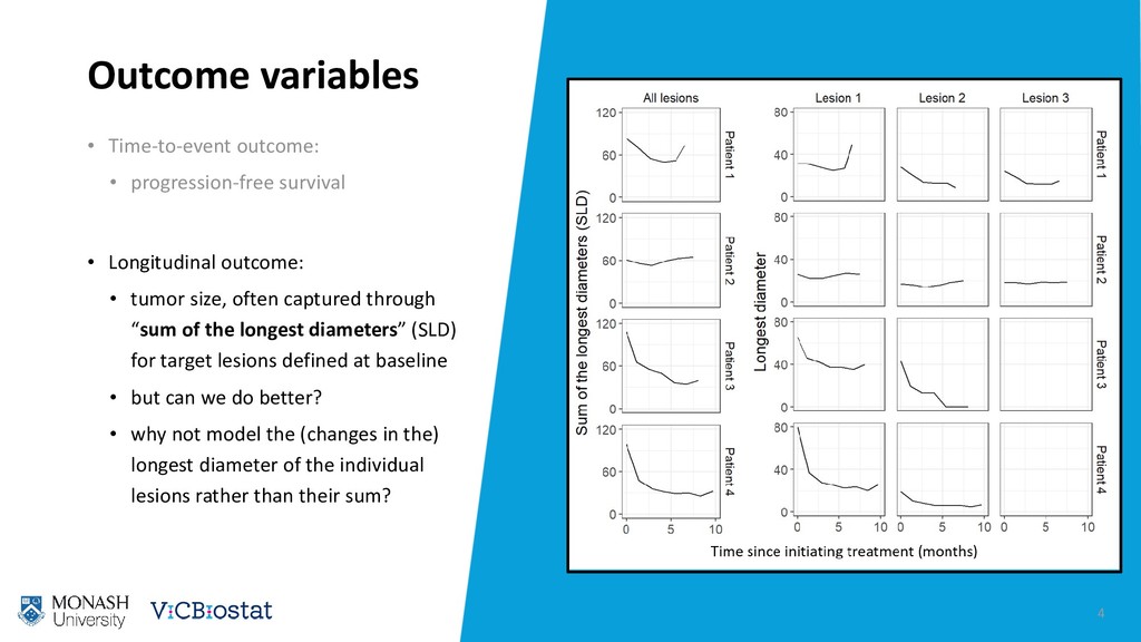
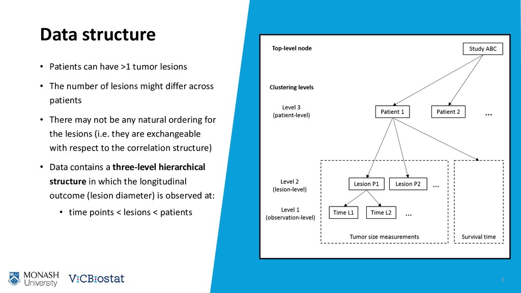
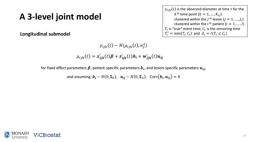
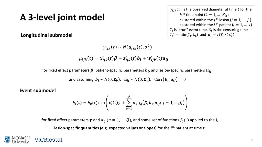
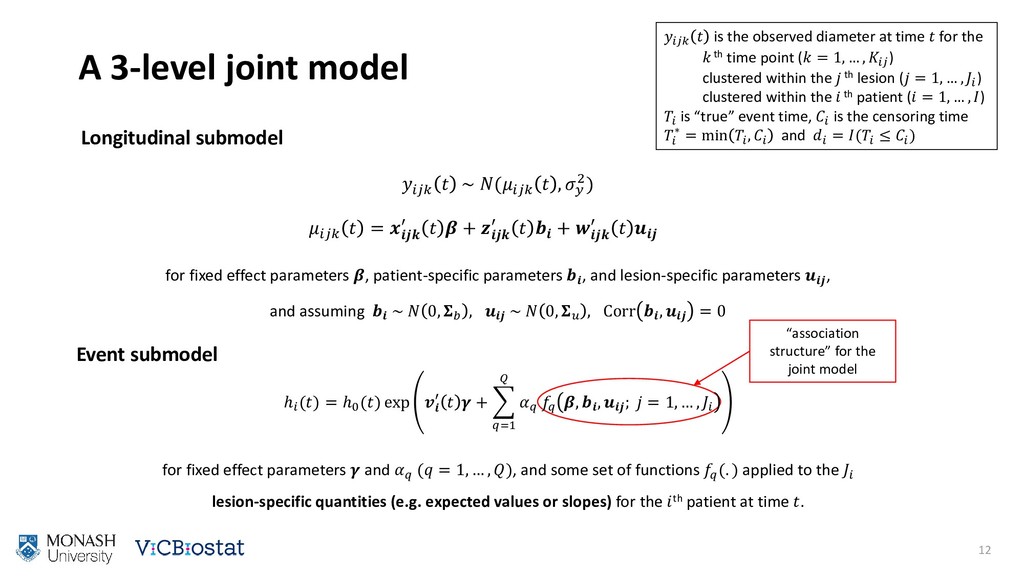
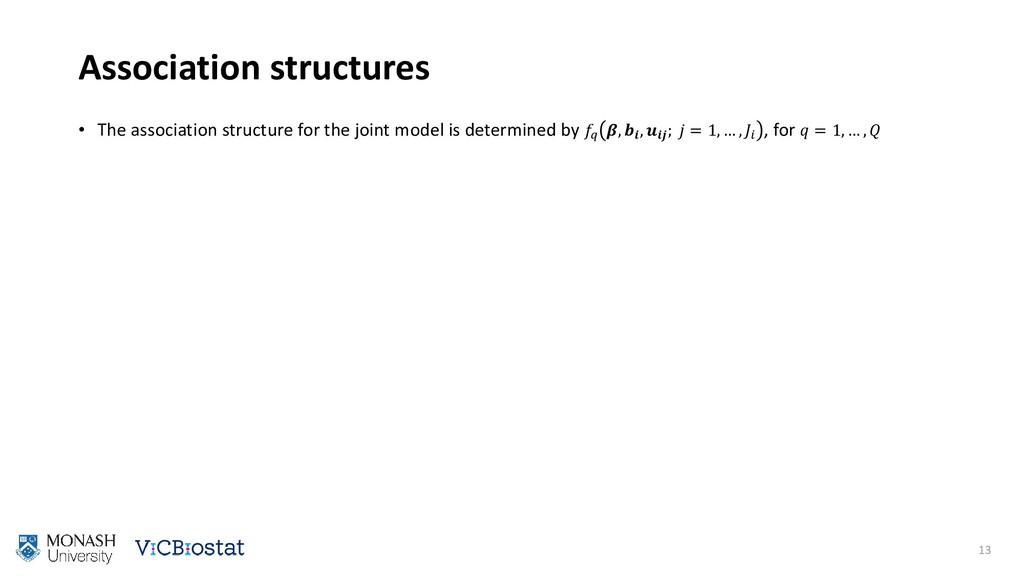
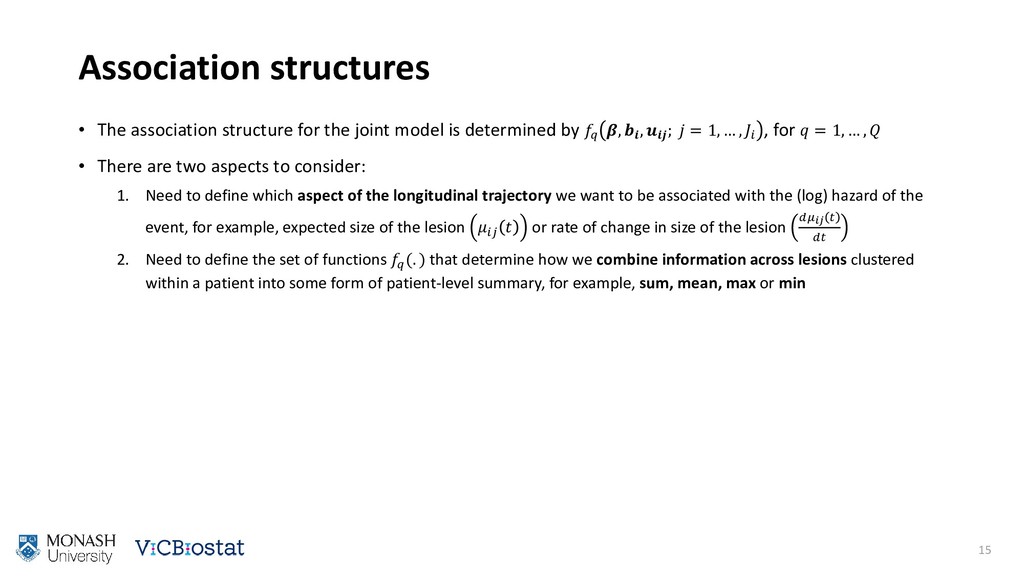
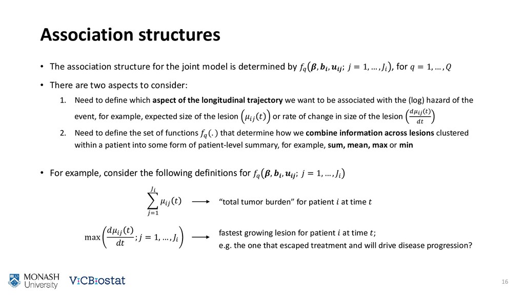
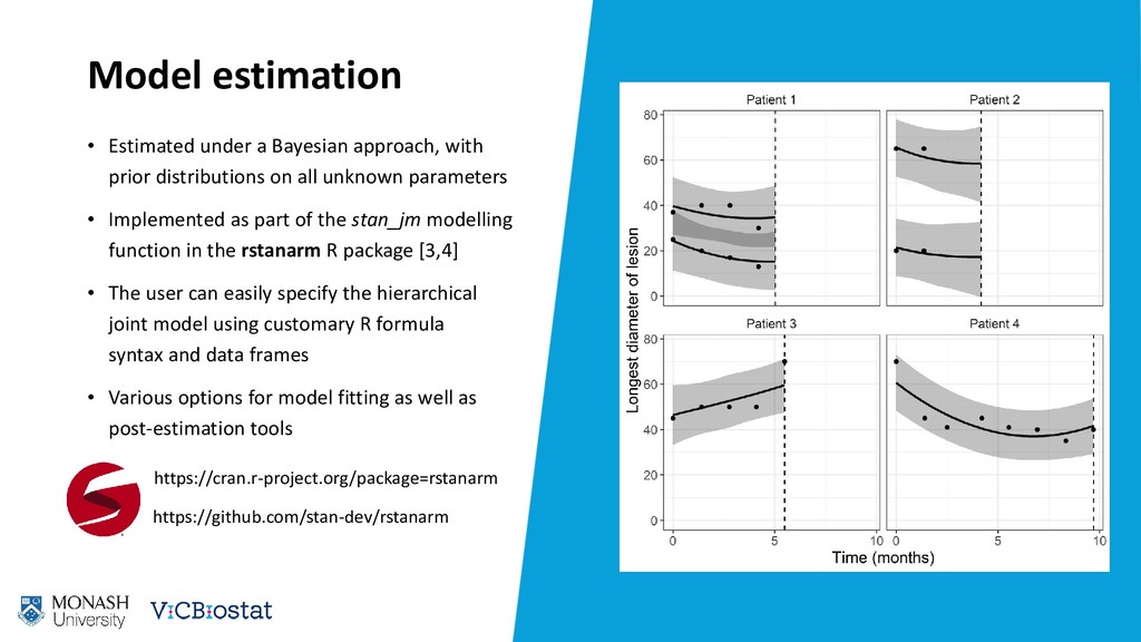
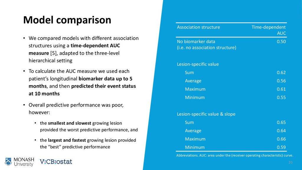
Joint modelling of longitudinal and time-to-event data has received much attention recently. Increasingly, extensions to standard joint modelling approaches are being proposed to handle complex data structures commonly encountered in applied research. In this paper we propose a joint model for hierarchical longitudinal and time-to-event data. Our motivating application explores the association between tumor burden and progression-free survival in non-small cell lung cancer patients. We define tumor burden as a function of the sizes of target lesions clustered within a patient. Since a patient may have more than one lesion, and each lesion is tracked over time, the data have a three-level hierarchical structure: repeated measurements taken at time points (level 1) clustered within lesions (level 2) within patients (level 3). We jointly model the lesion-specific longitudinal trajectories and patient-specific risk of death or disease progression by specifying novel association structures that combine information across lower level clusters (e.g. lesions) into patient-level summaries (e.g. tumor burden). We provide user-friendly software for fitting the model under a Bayesian framework. Lastly, we discuss alternative situations in which additional clustering factor(s) occur at a level higher in the hierarchy than the patient-level, since this has implications for the model formulation. To demonstrate the wider applicability of the methodological framework we describe additional settings in which this type of multilevel joint model data might be encountered, including examples from ophthalmology and meta-analysis.

Transcript

1. Joint longitudinal and time-to-event models for multilevel hierarchical data Sam Brilleman1,2, Michael J Crowther3, Margarita Moreno-Betancur2,4,5, Jacqueline Buros Novik6, James Dunyak7, Nidal Al-Huniti7, Robert Fox7, Rory Wolfe1,2 39th Conference of the International Society for Clinical Biostatistics (ISCB) Melbourne, Australia 26-30th August 2018 1 Monash University, Melbourne, Australia 3 University of Leicester, Leicester, UK 5 University of Melbourne, Melbourne, Australia 2 Victorian Centre for Biostatistics (ViCBiostat), Melbourne, Australia 4 Murdoch Childrens Research Institute, Melbourne, Australia 6 Icahn School of Medicine at Mount Sinai, New York, NY, USA 7 AstraZeneca, Waltham, MA, USA
2. Motivating application • Data from the Iressa Pan-Asia Study (IPASS) • phase 3 trial of N = 1,217 untreated non-small cell lung cancer (NSCLC) patients in East Asia randomized to either (i) gefitinib or (ii) carboplatin + paclitaxel [1] • primary outcome was progression-free survival • main trial results suggested that an epidermal growth factor receptor (EGFR) mutation was associated with treatment response (i.e. treatment by subgroup interaction) [2] • We performed a secondary analysis of data for the N = 430 (35%) patients with known EGFR mutation status • We used a joint modelling approach to explore how changes in tumor size are related to death or disease progression 2
3. Outcome variables • Time-to-event outcome: • progression-free survival 3
4. Outcome variables • Time-to-event outcome: • progression-free survival • Longitudinal outcome: • tumor size, often captured through “sum of the longest diameters” (SLD) for target lesions defined at baseline • but can we do better? • why not model the (changes in the) longest diameter of the individual lesions rather than their sum? 4
5. Data structure • Patients can have >1 tumor lesions • The number of lesions might differ across patients • There may not be any natural ordering for the lesions (i.e. they are exchangeable with respect to the correlation structure) • Data contains a three-level hierarchical structure in which the longitudinal outcome (lesion diameter) is observed at: • time points < lesions < patients 5
6. Joint modelling • Joint estimation of regression models which traditionally would have been estimated separately: • a mixed effects model for a longitudinal outcome (“longitudinal submodel”) • a time-to-event model for the time to an event of interest (“event submodel”) • the submodels are linked through shared parameters 6
7. Joint modelling • Joint estimation of regression models which traditionally would have been estimated separately: • a mixed effects model for a longitudinal outcome (“longitudinal submodel”) • a time-to-event model for the time to an event of interest (“event submodel”) • the submodels are linked through shared parameters • Most common shared parameter joint model has included one longitudinal outcome (a repeatedly measured “biomarker”) and one terminating event outcome 7
8. Joint modelling • Joint estimation of regression models which traditionally would have been estimated separately: • a mixed effects model for a longitudinal outcome (“longitudinal submodel”) • a time-to-event model for the time to an event of interest (“event submodel”) • the submodels are linked through shared parameters • Most common shared parameter joint model has included one longitudinal outcome (a repeatedly measured “biomarker”) and one terminating event outcome • However, a vast number of extensions have been proposed, for example: • competing risks, recurrent events, interval censored events, multiple longitudinal outcomes, … 8
9. Joint modelling • Joint estimation of regression models which traditionally would have been estimated separately: • a mixed effects model for a longitudinal outcome (“longitudinal submodel”) • a time-to-event model for the time to an event of interest (“event submodel”) • the submodels are linked through shared parameters • Most common shared parameter joint model has included one longitudinal outcome (a repeatedly measured “biomarker”) and one terminating event outcome • However, a vast number of extensions have been proposed, for example: • competing risks, recurrent events, interval censored events, multiple longitudinal outcomes, … • But a common aspect has been a two-level hierarchical data structure: • longitudinal biomarker measurements are observed at time points (level 1) < patients (level 2) 9
10. A 3-level joint model 10 is the observed diameter at time for the th time point ( = 1, … , ) clustered within the th lesion ( = 1, … , ) clustered within the th patient ( = 1, … , ) is “true” event time, is the censoring time ∗ = min , and = ( ≤ ) ~ ( , 2) = ′ + ′ + ′ for fixed effect parameters , patient-specific parameters , and lesion-specific parameters , and assuming ~ 0, , ~ 0, , Corr , = 0 Longitudinal submodel
11. ℎ () = ℎ0 () exp ′ + ෍ =1 , , ; = 1, … , for fixed effect parameters and ( = 1, … , ), and some set of functions (. ) applied to the lesion-specific quantities (e.g. expected values or slopes) for the th patient at time . A 3-level joint model 11 is the observed diameter at time for the th time point ( = 1, … , ) clustered within the th lesion ( = 1, … , ) clustered within the th patient ( = 1, … , ) is “true” event time, is the censoring time ∗ = min , and = ( ≤ ) ~ ( , 2) = ′ + ′ + ′ for fixed effect parameters , patient-specific parameters , and lesion-specific parameters , and assuming ~ 0, , ~ 0, , Corr , = 0 Longitudinal submodel Event submodel
12. A 3-level joint model 12 Event submodel is the observed diameter at time for the th time point ( = 1, … , ) clustered within the th lesion ( = 1, … , ) clustered within the th patient ( = 1, … , ) is “true” event time, is the censoring time ∗ = min , and = ( ≤ ) ~ ( , 2) = ′ + ′ + ′ for fixed effect parameters , patient-specific parameters , and lesion-specific parameters , and assuming ~ 0, , ~ 0, , Corr , = 0 Longitudinal submodel “association structure” for the joint model ℎ () = ℎ0 () exp ′ + ෍ =1 , , ; = 1, … , for fixed effect parameters and ( = 1, … , ), and some set of functions (. ) applied to the lesion-specific quantities (e.g. expected values or slopes) for the th patient at time .
13. Association structures • The association structure for the joint model is determined by , , ; = 1, … , , for = 1, … , 13
14. Association structures • The association structure for the joint model is determined by , , ; = 1, … , , for = 1, … , • There are two aspects to consider: 1. Need to define which aspect of the longitudinal trajectory we want to be associated with the (log) hazard of the event, for example, expected size of the lesion or rate of change in size of the lesion 14
15. Association structures • The association structure for the joint model is determined by , , ; = 1, … , , for = 1, … , • There are two aspects to consider: 1. Need to define which aspect of the longitudinal trajectory we want to be associated with the (log) hazard of the event, for example, expected size of the lesion or rate of change in size of the lesion 2. Need to define the set of functions (. ) that determine how we combine information across lesions clustered within a patient into some form of patient-level summary, for example, sum, mean, max or min 15
16. Association structures • The association structure for the joint model is determined by , , ; = 1, … , , for = 1, … , • There are two aspects to consider: 1. Need to define which aspect of the longitudinal trajectory we want to be associated with the (log) hazard of the event, for example, expected size of the lesion or rate of change in size of the lesion 2. Need to define the set of functions (. ) that determine how we combine information across lesions clustered within a patient into some form of patient-level summary, for example, sum, mean, max or min • For example, consider the following definitions for , , ; = 1, … , 16 ෍ =1 “total tumor burden” for patient at time max ; = 1, … , fastest growing lesion for patient at time ; e.g. the one that escaped treatment and will drive disease progression?
17. Model specification • Longitudinal submodel • Fixed effect covariates: • 3 category group variable (EGFR+; EGFR- with carboplatin plus paclitaxel; EGFR- with gefitinib) • Linear and quadratic terms for time (orthogonalised) • Interaction between group and the linear & quadratic terms • Random effect covariates: • Patient-level: random intercept • Lesion-level: random intercept, linear and quadratic terms for time 17
18. Model specification • Longitudinal submodel • Fixed effect covariates: • 3 category group variable (EGFR+; EGFR- with carboplatin plus paclitaxel; EGFR- with gefitinib) • Linear and quadratic terms for time (orthogonalised) • Interaction between group and the linear & quadratic terms • Random effect covariates: • Patient-level: random intercept • Lesion-level: random intercept, linear and quadratic terms for time • Event submodel • B-splines used to model the log baseline hazard • Fixed effect covariates: • 3 category physical functioning measure (normal activity; restricted activity; in bed >50% of the time) • Association structure: sum, mean, min, or max of the lesion-specific values and/or slopes 18
19. Model estimation • Estimated under a Bayesian approach, with prior distributions on all unknown parameters • Implemented as part of the stan_jm modelling function in the rstanarm R package [3,4] • The user can easily specify the hierarchical joint model using customary R formula syntax and data frames • Various options for model fitting as well as post-estimation tools 19 Model comparison • In our application we compared models with different association structures using a time-dependent AUC measure [3], adapted to the three-level hierarchical setting • To calculate the AUC measure we used each patient’s longitudinal biomarker data up to 5 months, and then predicted their event status at 10 months https://github.com/stan-dev/rstanarm https://cran.r-project.org/package=rstanarm
20. Model comparison • We compared models with different association structures using a time-dependent AUC measure [5], adapted to the three-level hierarchical setting • To calculate the AUC measure we used each patient’s longitudinal biomarker data up to 5 months, and then predicted their event status at 10 months • Overall predictive performance was poor, however: • the smallest and slowest growing lesion provided the worst predictive performance, and • the largest and fastest growing lesion provided the “best” predictive performance 20 Abbreviations. AUC: area under the (receiver operating characteristic) curve. Association structure Time-dependent AUC No biomarker data (i.e. no association structure) 0.50 Lesion-specific value Sum 0.62 Average 0.56 Maximum 0.61 Minimum 0.55 Lesion-specific value & slope Sum 0.65 Average 0.64 Maximum 0.66 Minimum 0.59
21. Summary • Joint modelling approaches have previously been limited to a two-level hierarchical data structure • However, many clinical research settings present us with data that has additional levels of clustering • Our proposed approach models the longitudinal measurements for lower-level clusters, and combines them into a patient-level summary that we assume is associated with the event rate • From an inferential perspective, the method allows for association structures that would not have otherwise been possible • From a model performance perspective, the method can potentially improve model fit since it provides greater flexibility, i.e. we can directly model the longitudinal trajectories for distinct lower- level units clustered within a patient • The method has been implemented in general-purpose, freely-accessible, user-friendly software 21
22. Thank you [1] Mok TS et al. Gefitinib or Carboplatin–Paclitaxel in Pulmonary Adenocarcinoma. New England Journal of Medicine. 2009; 361: 947– 957 [2] Fukuoka M et al. Biomarker Analyses and Final Overall Survival Results From a Phase III, Randomized, Open-Label, First-Line Study of Gefitinib Versus Carboplatin/Paclitaxel in Clinically Selected Patients With Advanced Non–Small-Cell Lung Cancer in Asia (IPASS). Journal of Clinical Oncology. 2011; 29: 2866–2874 [3] Stan Development Team. 2018. rstanarm: Bayesian applied regression modeling via Stan. R package version 2.17.4. http://mc- stan.org/rstanarm [4] Brilleman SL et al. Joint longitudinal and time-to-event models via Stan. In: Proceedings of StanCon 2018. Pacific Grove, CA, USA. DOI: 10.5281/zenodo.1284334 [5] Rizopoulos D. Dynamic Predictions and Prospective Accuracy in Joint Models for Longitudinal and Time-to-Event Data. Biometrics. 2011; 67: 819–829. 22 References sam.brilleman@monash.edu https://www.sambrilleman.com @sambrilleman