Upgrade to Pro — share decks privately, control downloads, hide ads and more …

Integration of Biological Knowledge in the Mixture of Gaussians Analysis of Genomic Clustering

Integration of Biological Knowledge in the Mixture of Gaussians Analysis of Genomic Clustering

Stelios Sfakianakis

November 03, 2010
Tweet

More Decks by Stelios Sfakianakis

Other Decks in Research

Transcript

  1. . . . . . . . . . .

    . . . Integration of Biological Knowledge in the Mixture-of-Gaussians Analysis of Genomic Clustering S. Sfakianakis1,2 M. Zervakis2 M. Tsiknakis1 D. Kafetzopoulos3 1Institute of Computer Science, Foundation for Research and Technology - Hellas 2Department of Electronic and Computer Engineering, Technical University of Crete 3Institute of Molecular Biology, Foundation for Research and Technology - Hellas November 3, 2010 Sfakianakis et al. (ECE) Integration of Biological Knowledge.. November 3, 2010 1 / 15
  2. . . . . . . Introduction Objective Early work

    in bioinformatics focused on the identification of a small number of infromative genes to discriminate between phenotypes or experimental conditions Instead we now see a shift to more integrated analysis of gene expression data, leading to the systems biology In this work we try to use existing biological knowledge to guide the analysis of gene expression data Sfakianakis et al. (ECE) Integration of Biological Knowledge.. November 3, 2010 2 / 15
  3. . . . . . . Methods Finite Models and

    the EM Finite Mixture Models Mixture models [McLachlan, 2000] present a probabilistic framework both for building complex probability distributions (e.g. density estimation) as linear combinations of simpler ones but also for clustering data (unsupervised learning) They present a “generative” model: a sample x x xj can have been generated by one of the g clusters or groups: f (x x xj ;Θ Θ Θ) = g ∑ i=1 πi fi (x x xj ;θi θi θi ) (1) where Θ Θ Θ is the collection of the unknown parameters πi that are usually referred as “mixing coefficients”, and θi θi θi , which are the parameters of the component densities fi . And also 0 ≤ πi ≤ 1 and ∑ g i=1 πi = 1. Sfakianakis et al. (ECE) Integration of Biological Knowledge.. November 3, 2010 3 / 15
  4. . . . . . . Methods Finite Models and

    the EM Gaussian Mixture Models In the Gaussian Mixture Models (GMM) each of the component probability distributions is Gaussian but with different parameters: fi (x x xj ;θ θ θi ) = N(x x xj ;µ µ µi ,Σ Σ Σi ) ≡ 1 √ (2π)p|Σ Σ Σi | e−1 2 (x x xj −µ µ µi )T Σ Σ Σ−1 i (x x xj −µ µ µi ) (2) f (x x xj ;Θ Θ Θ) = g ∑ i=1 πi N(x x xj ;µ µ µi ,Σ Σ Σi ) (3) There’s an efficient iterative algorithm called Expectation Maximization (EM) to compute the models’ parameters of GMM [Dempster, 1977] Sfakianakis et al. (ECE) Integration of Biological Knowledge.. November 3, 2010 4 / 15
  5. . . . . . . Methods Finite Models and

    the EM EM for GMM Initialize the models’ parameters µ µ µi , Σi , πi E-step. Compute the support (or “responsibility”) each sample provides to a given component density as the conditional probability τji ≡ Pr(zji = 1|x x xj ;Θ Θ Θcur) = πcur j N(x x xj ;µ µ µcur i ,Σ Σ Σcur i )) ∑ g c=1 πcur c N(x x xj ;µ µ µcur c ,Σ Σ Σcur c )) (4) M-step. µ µ µnew i = ∑ N j=1 τijx x xj ∑ N i=1 τji Σ Σ Σnew i = ∑ N j=1 τji (x x xj − µ µ µnew i )(x x xj − µ µ µnew i )T ∑ N j=1 τji πnew i = 1 N N ∑ j=1 τji (5) Sfakianakis et al. (ECE) Integration of Biological Knowledge.. November 3, 2010 5 / 15
  6. . . . . . . Methods Stratified Model Integrating

    Biological Knowledge: the Stratified model The genes can be classifed into K “functional groups” e.g. based on the Gene Ontology or the Pathways We assume genes categorized into the same functional group are dependent whereas genes in different groups are independent For Gaussian distributions independence is equivalent to uncorrelatedness and therefore we introduce the following “stratified” model for the covariance matrix: Σ Σ Σ =        Σ Σ Σ(1) 0 0 0 · · · 0 0 0 0 0 0 0 0 0 Σ Σ Σ(2) · · · 0 0 0 0 0 0 . . . . . . ... . . . . . . 0 0 0 0 0 0 · · · Σ Σ Σ(K) 0 0 0 0 0 0 0 0 0 · · · 0 0 0 D D D(r)        (6) where each of Σ Σ Σ(k) is the (unconstrained) covariance (sub)matrix for the genes belonging to the k group, and D D D is the diagonal covariance matrix of the r genes that do not belong to any group. Sfakianakis et al. (ECE) Integration of Biological Knowledge.. November 3, 2010 6 / 15
  7. . . . . . . Methods Stratified Model The

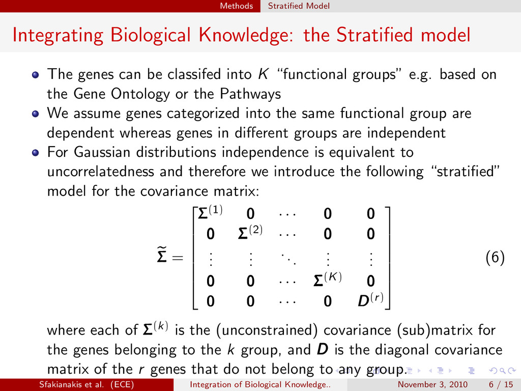
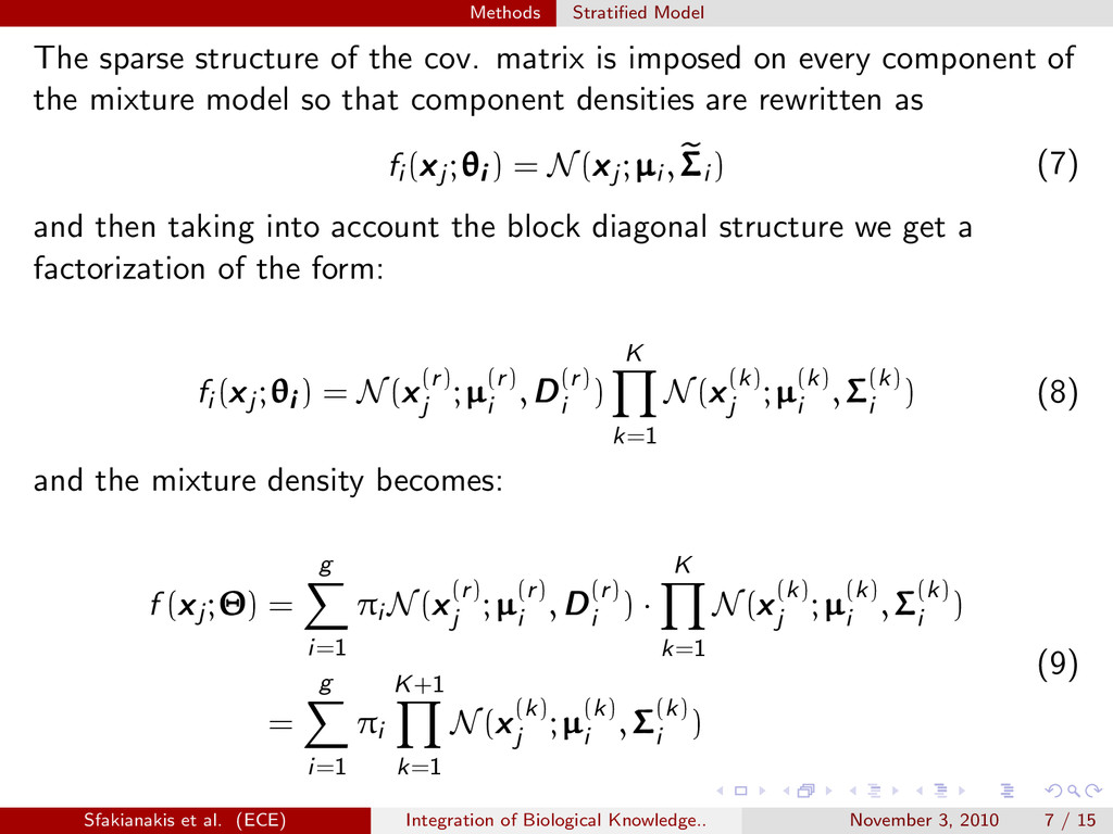
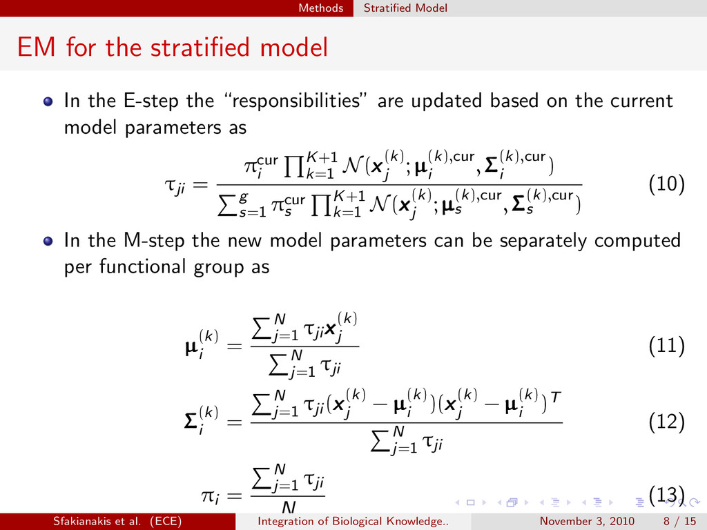
    sparse structure of the cov. matrix is imposed on every component of the mixture model so that component densities are rewritten as fi (x x xj ;θi θi θi ) = N(x x xj ;µ µ µi ,Σ Σ Σi ) (7) and then taking into account the block diagonal structure we get a factorization of the form: fi (x x xj ;θi θi θi ) = N(x x x(r) j ;µ µ µ(r) i ,D D D(r) i ) K ∏ k=1 N(x x x(k) j ;µ µ µ(k) i ,Σ Σ Σ(k) i ) (8) and the mixture density becomes: f (x x xj ;Θ Θ Θ) = g ∑ i=1 πi N(x x x(r) j ;µ µ µ(r) i ,D D D(r) i ) · K ∏ k=1 N(x x x(k) j ;µ µ µ(k) i ,Σ Σ Σ(k) i ) = g ∑ i=1 πi K+1 ∏ k=1 N(x x x(k) j ;µ µ µ(k) i ,Σ Σ Σ(k) i ) (9) Sfakianakis et al. (ECE) Integration of Biological Knowledge.. November 3, 2010 7 / 15
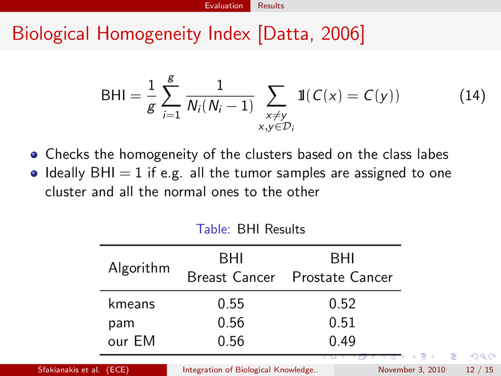
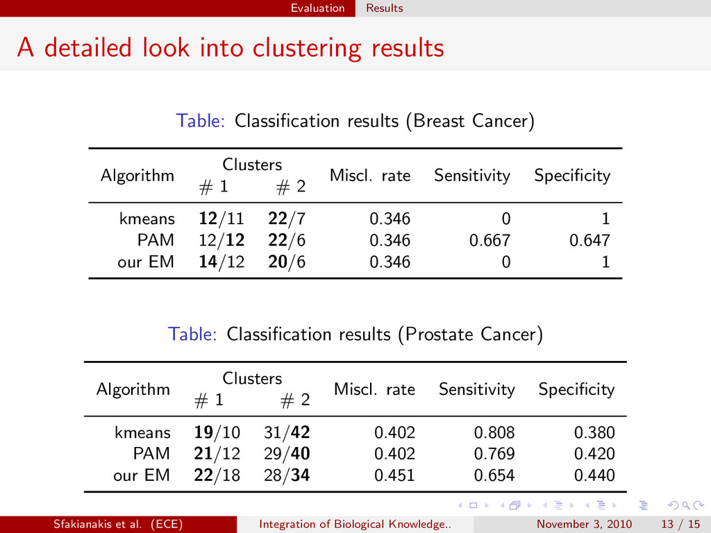
  8. . . . . . . Methods Stratified Model EM

    for the stratified model In the E-step the “responsibilities” are updated based on the current model parameters as τji = πcur i ∏ K+1 k=1 N(x x x(k) j ;µ µ µ(k),cur i ,Σ Σ Σ(k),cur i ) ∑ g s=1 πcur s ∏ K+1 k=1 N(x x x(k) j ;µ µ µ(k),cur s ,Σ Σ Σ(k),cur s ) (10) In the M-step the new model parameters can be separately computed per functional group as µ µ µ(k) i = ∑ N j=1 τjix x x(k) j ∑ N j=1 τji (11) Σ Σ Σ(k) i = ∑ N j=1 τji (x x x(k) j − µ µ µ(k) i )(x x x(k) j − µ µ µ(k) i )T ∑ N j=1 τji (12) πi = ∑ N j=1 τji N (13) Sfakianakis et al. (ECE) Integration of Biological Knowledge.. November 3, 2010 8 / 15
  9. . . . . . . Evaluation Data sets Evaluation

    In order to perform some evaluation of our method two data sets are used: A Breast Cancer data set [Huang, 2003] where there exist 52 samples with 18 samples exhibit recurrence of tumor and 34 do not. A Prostate Cancer data set [Singh, 2002] where there exist 52 tumor samples and 50 normal samples. Both are based on the AffymetrixTM hgu95av2 platform, containing 12625 probesets that are preprocessed using the GCRMA normalization and summarization methods. Sfakianakis et al. (ECE) Integration of Biological Knowledge.. November 3, 2010 9 / 15
  10. . . . . . . Evaluation Data sets Defining

    functional groups: KEGG Pathways Table: The KEGG pathways used in the tests Pathway id Pathway name 1 04115 p53 signaling pathway 2 04210 Apoptosis 3 04370 VEGF signaling pathway 4 05010 Alzheimer’s disease 5 05012 Parkinson’s disease 6 05014 Amyotrophic lateral sclerosis (ALS) 7 05016 Huntington’s disease 8 05200 Pathways in cancer 9 05210 Colorectal cancer 10 05212 Pancreatic cancer 11 05213 Endometrial cancer 12 05215 Prostate cancer 13 05222 Small cell lung cancer 14 05223 Non-small cell lung cancer 15 05416 Viral myocarditis Sfakianakis et al. (ECE) Integration of Biological Knowledge.. November 3, 2010 10 / 15
  11. . . . . . . Evaluation Data sets Comparison

    of clustering results Algorithms: k-means, PAM, and our stratified EM “Hard” clustering can be done by assigning a sample to the cluster it mostly supports (i.e. based on the value of τji ) Comparison of clustering results The “true” underlying clusters are unknown We use the class labels to validate and evaluate the cluster results Because both datasets have a binary classification, we request the identification of g = 2 clusters Sfakianakis et al. (ECE) Integration of Biological Knowledge.. November 3, 2010 11 / 15
  12. . . . . . . Evaluation Results Biological Homogeneity

    Index [Datta, 2006] BHI = 1 g g ∑ i=1 1 Ni (Ni − 1) ∑ x=y x,y∈Di 1 I(C(x) = C(y)) (14) Checks the homogeneity of the clusters based on the class labes Ideally BHI = 1 if e.g. all the tumor samples are assigned to one cluster and all the normal ones to the other Table: BHI Results Algorithm BHI BHI Breast Cancer Prostate Cancer kmeans 0.55 0.52 pam 0.56 0.51 our EM 0.56 0.49 Sfakianakis et al. (ECE) Integration of Biological Knowledge.. November 3, 2010 12 / 15
  13. . . . . . . Evaluation Results A detailed

    look into clustering results Table: Classification results (Breast Cancer) Algorithm Clusters Miscl. rate Sensitivity Specificity # 1 # 2 kmeans 12/11 22/7 0.346 0 1 PAM 12/12 22/6 0.346 0.667 0.647 our EM 14/12 20/6 0.346 0 1 Table: Classification results (Prostate Cancer) Algorithm Clusters Miscl. rate Sensitivity Specificity # 1 # 2 kmeans 19/10 31/42 0.402 0.808 0.380 PAM 21/12 29/40 0.402 0.769 0.420 our EM 22/18 28/34 0.451 0.654 0.440 Sfakianakis et al. (ECE) Integration of Biological Knowledge.. November 3, 2010 13 / 15
  14. . . . . . . Conclusions Conclusions Integration of

    biological knowledge is a “hot” area Such knowledge can be used to overcome computational deficiencies and also improve the results and the validity of the methods The stratified model can be seen as a middle solution between choosing the full sample covariance matrix, which can lead to an ill-posed inverse problem, and a lower dimensional diagonal covariance matrix. Sfakianakis et al. (ECE) Integration of Biological Knowledge.. November 3, 2010 14 / 15
  15. . . . . . . Conclusions Limitations and future

    work The outcome of the experiments are not very informative on the validity of the described approach and further testing will be conducted in the future. The statified model that we defined assumes the independence of the uncategorized genes, an assumption that is definitely far from the truth. It can be the case that certain genes can have more than one functional annotation or participate in more than one category or pathway. Improve the performance and robustness and study of the convergence properties Sfakianakis et al. (ECE) Integration of Biological Knowledge.. November 3, 2010 15 / 15