Upgrade to Pro — share decks privately, control downloads, hide ads and more …

Stacking of network based classifiers with application in Breast Cancer classification

Stacking of network based classifiers with application in Breast Cancer classification

Stelios Sfakianakis

April 01, 2016
Tweet

More Decks by Stelios Sfakianakis

Other Decks in Research

Transcript

  1. Stacking of network based classifiers with application in Breast Cancer

    classification S. Sfakianakis, E.S. Bei and M. Zervakis Department of Electronic and Computer Engineering, Technical University of Crete 1
  2. Network-based Medicine • Systems Biology and network- based approaches are

    essential for the understanding of the biological processes and mechanisms underlying disease progression • Biological networks include Gene interaction and Protein-Protein interaction networks • In the present study we propose a novel approach for building predictive models that use the underlying topological information of biological networks in an adaptive way. 2
  3. Aim • Build a predictive model for the classification of

    unknown cases (biological samples) into predefined categories (e.g. metastatic versus non- metastatic samples) • Specific application domain : Breast Cancer, starting from an initial list of marker genes for the characterization of Circulating Tumor Cells (Sfakianakis, 2014) 3 based schemes, but our aim is to construct an adaptive, gene signature initialized, and biologically driven classifier. The results are indeed promising and make stronger the selection of our initial gene list used for the initialization, but further evaluation, tuning, and validation are needed. ACKNOWLEDGMENTS This research is partially supported by the “ONCOSEED” project funded by the NSRF2007-13 Program of the Greek Ministry of Education, Lifelong Learning and Religious Af- fairs. CONFLICT OF INTEREST The authors declare that they have no conflict of interest. REFERENCES 1. Barab´ asi A-L, Gulbahce N, Loscalzo J. Network medicine: a network-based approach to human disease Nature Reviews Genetics. 2011;12:56–68. 2. Vanunu O, Magger O, Ruppin E, Shlomi T, Sharan R. Associating Genes and Protein Complexes with Disease via Network Propagation PLoS Comput Biol. 2010;6:e1000641. 3. Vidal M, Cusick M E, Barab´ asi A-L. Interactome Networks and Human Disease Cell. 2011;144:986–998. 4. Kohavi R, John G H. Wrappers for feature subset selection Artificial intelligence. 1997. 5. Sfakianakis S, Bei E S, Zervakis M, Vassou D, Kafetzopoulos D. On the Identification of Circulating Tumor Cells in Breast Cancer Biomedical and Health Informatics, IEEE Journal of. 2014;18:773–782. 6. Das J, Yu H. HINT: High-quality protein interactomes and their appli- cations in understanding human disease BMC Systems Biology. 2012. 7. Segal E, Friedman N, Kaminski N, Regev A, Koller D. From signatures (Sfakianakis, 2014)
  4. Circulating Tumor Cells • Tumor cells are released from tumors

    into blood stream • They have a key role in future metastasis • Approximately 1 CTC in a billion blood cells! C. L. Chaffer and R. A. Weinberg, “A Perspective on Cancer Cell Metastasis,” Science, vol. 331, no. 6024, pp. 1559–1564, Mar. 2011. 4
  5. Inputs • A list of m genes samples), an additional

    set of gene expression val {( x x xj,yj) ,x x xj 2 Rk ,yj = ± 1,1 6 j 6 N } are used in vised learning setting. Our approach is based on the following two main • For each gene in the initial list L we compute th imities to any other gene in the biological netwo • The distances between the genes in the initial s n values D = sed in a super- main steps: entries in this matrix we tran tances” so that two genes wit are considered closed to eac distance matrix provides the other by taking into account • Gene expression data set: omising results in . orks, page rank, ancer is concep- genetic, epige- mical responses, ules. A network- g the biological ase progression. tion, in a binary classification problem. II. METHODS The starting point of our work is a L = { gi,1 6 i 6 m }, alongside with a G = ( V,E ), where V is the set of vertice genes, and E is the list of edges connectin the initial set L of genes we are using th from our earlier work [5]. These genes of the multiple comparisons between nor samples in blood and breast tissues. The we use is HINT [6], a protein-protein inter consists, at the time of this writing, of ar • A biological network with genes as vertices (V) and their interactions as the edges (E) connecting them: sible way the re- proach therefore the initial list of guarantees. Our mising results in orks, page rank, each initial candidate biomar pendently to build the same n tive is then to build a classifie of these “base” classifiers in o tion, in a binary classification II. ME The starting point of ou L = { gi,1 6 i 6 m }, alongs G = ( V,E ), where V is the s 5
  6. Rationale • The list of m “seed” genes represent a

    candidate “gene signature” for the characterization of a medical condition or a disease such as cancer, or a biological phenotype • We aim at using each of these genes as centers for the construction of independent “classifiers” using the network topology as guidance for the selection of genes that will be included in the classifier built around those centers. • The classifiers are then combined into a higher level classifier in order to produce more robust classification performance than the initial list of genes. 6
  7. Methodology • For each gene in the initial list L

    we compute their proximities to any other gene in the biological network G. • The distances between the genes in the initial set L and any other gene in the network are then used to build a two level hierarchical meta-classifier using the training set D 7
  8. Computing Gene Proximities • “Random walks” in Graph with Restart

    sider random walks with restart [11]: given a parameter that corresponds to the probability that there’s no tran- sition from one node of the graph to any other, the proba- bility distribution for every node in the graph at time t + 1 is given by: P P Pt+1 = P P P0 +( 1 - ) W W WP P Pt (1) where P P P0 is the initial assignment of weights in the nodes of the graph, and W W W is the “normalized adjacency matrix” of the graph, i.e. W W Wi,j = 1 deg(j) if node i directly interacts with node j, 0 otherwise dom walks in graphs with restart [9, 10]. In more detail the proposed methodology is as follows: • Taking as input the gene interaction network G, we con- sider random walks with restart [11]: given a parameter that corresponds to the probability that there’s no tran- sition from one node of the graph to any other, the proba- bility distribution for every node in the graph at time t + 1 is given by: P P Pt+1 = P P P0 +( 1 - ) W W WP P Pt (1) where P P P0 is the initial assignment of weights in the nodes of the graph, and W W W is the “normalized adjacency matrix” of the graph, i.e. W W Wi,j = 1 deg(j) if node i directly interacts with node j, 0 otherwise where deg( j ) is the degree of a node, that is the number of genes adjacent to it. When the graph is connected then after many transitions the steady state condition P P Pt+1 = P P Pt ⌘ P P P gives: of genes that are ferent classifiers f collectively can in is a typical applica the output of the voting (majority w more authority tha gression problems proaches taking ad (Boostrap aggrega final classifier. An alternative w introduced by Wol eralization” or “sta classifiers (or “gen a new training set f sic idea is to train the original trainin for training the sec outputs of the firs tures while the ori the new training da In our case, w proach as follows: where is the initial assignment of weights in the nodes of the Graph, is the probability of starting again from the initial state and that corresponds to the probability that there’s no tra sition from one node of the graph to any other, the prob bility distribution for every node in the graph at time t + is given by: P P Pt+1 = P P P0 +( 1 - ) W W WP P Pt ( where P P P0 is the initial assignment of weights in the nod of the graph, and W W W is the “normalized adjacency matri of the graph, i.e. W W Wi,j = 1 deg(j) if node i directly interacts with node 0 otherwise where deg( j ) is the degree of a node, that is the numb • In the steady state: where P P P0 is the initial assignment of weights in the nodes f the graph, and W W W is the “normalized adjacency matrix” f the graph, i.e. W W Wi,j = 1 deg(j) if node i directly interacts with node j, 0 otherwise where deg( j ) is the degree of a node, that is the number f genes adjacent to it. When the graph is connected then fter many transitions the steady state condition P P Pt+1 = Pt ⌘ P P P gives: P P P = ( I I I -( 1 - ) W W W )-1 P P P0 (2) as input the gene interaction network G, we con- ndom walks with restart [11]: given a parameter orresponds to the probability that there’s no tran- om one node of the graph to any other, the proba- stribution for every node in the graph at time t + 1 by: P P Pt+1 = P P P0 +( 1 - ) W W WP P Pt (1) 0 is the initial assignment of weights in the nodes raph, and W W W is the “normalized adjacency matrix” raph, i.e. 1 deg(j) if node i directly interacts with node j, collectiv is a typic the outp voting (m more aut gression proaches (Boostra final clas An al introduc eralizatio classifier a new tra sic idea the origi 8
  9. • The following matrix is independent of the initial weights:

    eg( j ) is the degree of a node, that is the number adjacent to it. When the graph is connected then ny transitions the steady state condition P P Pt+1 = gives: P P P = ( I I I -( 1 - ) W W W )-1 P P P0 (2) ion 2 the matrix ( I I I - ( 1 - ) W W W )-1 ⌘ M M M is stic matrix independent of the initial weights P P P0 ures the probability of transitions (in one or more om any node in the graph to any other node (in- itself). By taking the negative logarithm of the outputs of tures while the new tra In our c proach as f • Each L of the i as dete 1Using th reciprocal) is “manageable” and captures the probability of transitions (in one or more steps) from any node in the graph to any other node (including itself) • The negative logarithm of this stochastic matrix can be considered a matrix of distances between genes 9
  10. Ensemble of network classifiers • Two level classification scheme based

    on “Stacked generalization” (Wolpert, 1992) • Each Level 0 classifier is built from a neighborhood from the genes that are most “closed” to the initial lists of m genes • Level 1 classifier combines the estimations of the lower level classifiers Figure 1: Stacked generalization or 2-level “stacking” of classifiers. The classifiers at the first level (Level 0) take as input the input cases and each one of them produces a prediction. The predictions of the first level classifiers are then given as input to the second level (Level 1) classifier 10
  11. • Each Level 0 classifier is built by selecting the

    genes closer to in an adaptive manner: How many neighbors to include is determined by an internal cross validation scheme • Different values of radius of the “open ball” centered in the “seed gene” are tried, using the Logistic Regression • The Level 1 classifier is a Random Forrest classifier and is trained using Leave-One-Out 11
  12. Experiments • Publicly available dataset GSE45965 consists of 67 gene

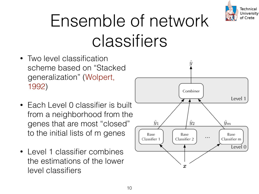
    expression profiles from peripheral blood, circulating cancer, breast cancer tissue, and normal epithelia • Probes are summarized according to UniGene clusters : Stacked generalization or 2-level “stacking” of classifiers. The s at the first level (Level 0) take as input the input cases and each them produces a prediction. The predictions of the first level rs are then given as input to the second level (Level 1) classifier (“combiner”) that provides the final prediction. s trained using Logistic Regression. The rationale his choice is twofold: First, logistic regression pro- s a probabilistic output, i.e. a level of confidence that nput sample belongs to the “positive” class (e.g. a or prognosis” group) that can be used as a numeri- eature for the second level classifier. Secondly, the abilistic output of a logistic regression classifier is lly well calibrated since it optimizes directly the log [18]. The choice of how many neighbors to consider each gi , which equivalently means the radius of the en ball” [19] centered at gi , is determined by an in- al cross validation. In this cross validation, increasing es of the radius r , that is the distance from the center e gi , are used and the subset of genes contained in said distance are checked in terms of the impact on sification performance as measured by the Matthews elation coefficient [20]. The different values of r tried A. Data We have used the recently available data set of Lang e al [21] to test the proposed two-level classification approac This data set is available as three “sub-series” in the Gen Expression Omnibus (GEO) public database as the “supe series” GSE45965 2. It consists of 67 gene expression pro files from peripheral blood, circulating cancer, breast cance tissue, and normal epithelia, as shown in Table 1. Table 1: Number of sample and characteristics of the public dataset GSE45965 Phenotype Number of samples Normal Peripheral Blood 8 Breast Cancer Tumor 50 Circulating Tumor Cells 5 Normal Epithelia 4 For the proper annotation of the gene probes in the data s we have used the UniGene database3 to perform mapping from the GeneBank identifiers to the Entrez Gene ids an gene symbols. Probes that dont’t have a UniGene annotatio or that have not been measured in all samples were remove For the case where multiple probes map to the same Entre Gene identifier the average (mean) expression value was ca culated and used in the downstream analysis. After this an notations and summarization step, we are left with aroun 15,000 unique genes. http://www.ncbi.nlm.nih.gov/geo/query/acc.cgi? acc=GSE45965 cate” instead of just considering their immediate neigh- We then consider a set of input genes that are used as for building a corresponding set of “base classifiers” d on the direct or indirect interactions the seeds have other genes. The base classifiers are subsequently used ain a second level classifier that can potentially com- ntelligently the successes and failures of them. The im- entation is based on the “scikit-learn” machine learn- ramework for Python [27] and all the code and the can be found at https://github.com/sgsfak/ net_stacking . e use of biological networks and random walks in hs have been studied in multiple publications [28, 29, 1]. Especially HotNet2 [29] uses similar random walk- d schemes, but our aim is to construct an adaptive, gene ture initialized, and biologically driven classifier. The s are indeed promising and make stronger the selection r initial gene list used for the initialization, but further ation, tuning, and validation are needed. ACKNOWLEDGMENTS is research is partially supported by the “ONCOSEED” ct funded by the NSRF2007-13 Program of the Greek stry of Education, Lifelong Learning and Religious Af- CONFLICT OF INTEREST Reviews Cancer. 2007;7:545–553. 9. Chung F. The heat kernel as the pagerank of a graph Proceedings of the National Academy of Sciences of the United States of America. 2007;104:19735–19740. 10. Can T, C ¸ amolu O, Singh A K. Analysis of protein-protein interaction networks using random walks in Proceedings of the 5th international workshop on Bioinformatics:61–68ACM 2005. 11. Lovasz L. Random walks on graphs: A survey Combinatorics. 1993. 12. Kittler J, Hatef M, Duin R P W, Matas J. On Combining Classifiers. IEEE Trans. Pattern Anal. Mach. Intell. (). 1998;20:226–239. 13. Dietterich T G. Ensemble Methods in Machine Learning. Multiple Classifier Systems. 2000:1–15. 14. Schapire R E. The strength of weak learnability Machine learning. 1990;5:197–227. 15. Freund Y, Schapire R E. A decision-theoretic generalization of on-line learning and an application to boosting Journal of computer and system sciences. 1997;55:119–139. 16. Breiman L. Bagging predictors Machine learning. 1996. 17. Wolpert D H. Stacked generalization Neural Networks. 1992;5:241– 259. 18. Bishop C. Pattern recognition and machine learning. New York: Springer 2006. 19. Rosenlicht M. Introduction to analysis. New York: Dover 1986. 20. Powers D M. Evaluation: from precision, recall and F-measure to ROC, informedness, markedness and correlation Journal of Machine Learn- ing Technologies. 2011;2:37–63. 21. Lang J E, Scott J H, Wolf D M, et al. Expression profiling of circulat- ing tumor cells in metastatic breast cancer Breast cancer research and treatment. 2015;149:121–131. 22. Fawcett T. An introduction to ROC analysis Pattern Recognition Let- ters. 2006;27:861–874. 23. Breiman L. Random Forests Machine Learning. 2001;45:5–32. 24. Subramanian A, Tamayo P, Mootha V K, et al. Gene set enrichment analysis: A knowledge-based approach for interpreting genome-wide expression profiles Proceedings of the National Academy of Sciences of the United States of America. 2005;102:15545–15550. 25. Mosca E, Alfieri R, Merelli I, Viti F, Calabria A, Milanesi L. A mul- tilevel data integration resource for breast cancer study BMC Systems Biology. 2010;4:76. 26. Chuang H-Y, Lee E, Liu Y-T, Lee D, Ideker T. Network-based classifi- 12
  13. Comparisons • We focus on the CTC vs Peripheral Blood

    (PB) and Breast Cancer vs PB comparisons • Metric: Area Under the ROC Curve (AUC) • For each of the two comparisons we performed a “repeated hold- out” evaluation process • “stratified” split of the randomly shuffled dataset, yielding a training set (70% of the samples) and a testing set (30%). • Repeated 100 times • Compare with SVMs and Logistic Regression fied” split of the randomly shuffled dataset is done. In each it- eration the training set consists of the 70% of the samples and the rest 30% is used for testing the trained classifiers. We re- peat the same process 100 times and each time we record the AUC achieved by each classifier. The final score of each clas- sification method is the average of the AUC scores achieved in each random split. The results are shown in Table 2. Table 2: Average AUC scores Classification method CTC versus PB (with gene se- lection) BC versus PB (with gene se- lection) Random Forest 0.830 (0.885) 0.921 (0.927) SVC-RBF 0.980 (0.995) 0.952 (0.995) Logistic regression with the biomarkers of [5] 0.932 0.979 Subnetwork Stacking 0.950 0.955 The Table 2 contains also the performance results for the Random Forest and the SVM rows when we perform a fea- ture (gene) selection preprocessing step, as follows: From each iteration we keep the most important genes as reported by the Random Forest classifier. The union of all these “im- portant” genes yield 306 genes in the CTC versus peripheral blood comparison and 455 genes in the peripheral blood ver- sus Breast cancer comparison. We then repeat the evaluation 13 (Sfakianakis, 2014)
  14. Significant Neighborhoods • In each random split of the data

    into training and testing sets during the iterated hold-out evaluation process, we normalize the importances of the base classifiers based on the performance of the whole 2-level classifier in the test set, as follows In the proposed stacked generalization methodology the fea- tures used are the predictions of the base classifiers and therefore they measure, indirectly, the classification ability of the genes selected in the neighborhood of the corresponding seeding gene. We take advantage of the iterated hold-out evaluation pro- cess so that in each random split of the data into training and testing sets we normalize the importances of the base classi- fiers based on the performance of the whole 2-level classifier in the test set, as follows: ^ g k i = AUCi ⇤ g k i where AUCi is the performance of the stacking classifier in the i -th iteration as measured in terms of the area under the ROC curve, g k i is the importance score of the k base classi- fier as reported by the random forest in the i -th iteration, and k • We then compute the mean over all iterations: e they measure, indirectly, the classification ability of es selected in the neighborhood of the corresponding gene. ake advantage of the iterated hold-out evaluation pro- hat in each random split of the data into training and ets we normalize the importances of the base classi- ed on the performance of the whole 2-level classifier st set, as follows: ^ g k i = AUCi ⇤ g k i AUCi is the performance of the stacking classifier in iteration as measured in terms of the area under the rve, g k i is the importance score of the k base classi- eported by the random forest in the i -th iteration, and e corresponding normalized importance of the base r. Computing the mean ^ gi = PK k=1 ^ g k i /K over all it- we find the results shown in Fig. 2. 14
  15. Genes most commonly selected per seed in the CTC versus

    PB comparison 16 https://git.io/vzlD8
  16. Genes most commonly selected per seed in the PB versus

    BC comparison 17 https://git.io/vzlD8
  17. Biological Evaluation • A number of breast cancer-related genes are

    to a greater or lesser degree interconnected with a) family members of oncogenes, tumor suppressors, transcription factors, protein kinases etc, and b) expression-responsive genes that can be involved in disease in many different ways: • A significant number of oncogenes (e.g. AKT1, JUN, CDK4, CREB1), and tumor suppressor genes (e.g. TNFAIP3, SMAD4, CDKN2A), as well as translocated cancer genes (e.g. CIC, MAFB) and transcription factors (e.g. CREB5, FOS, ESR1) • Breast Cancer-related genes: e.g. SREBF2, BECN1, GRB2, MAPK6, CASP3 • Expression-responsive genes: differentially expressed in CTC versus PB and/or CTC versus BC, according to the work of (Lang et. al, 2015), e.g. TMED10, TYROBP, PRKAR1A, GLO1, HNRNPU, JUNB, PRDX 18
  18. Concluding remarks • We present a two level classification scheme

    combining information from Biological Networks in a data-driven and adaptive methodology • Results are indeed encouraging and validate our previous findings (Sfakianakis, 2014) • Code available at https://github.com/sgsfak/ subnet_stacking 19
  19. 20