L23 chromatin states

BMMB 554 lecture 23

Transcript

1. L23: CHROMATIN STATE ANALYSIS Foundations in Data Driven Life Sciences BMMB 554
2. Learning objectives • Introduce Hidden Markov Models (HMMs) for biological sequence annotation. • Understand the concept of chromatin states as combinatorial patterns of regulatory signals. • Learn how HMMs can be applied to annotate regulatory features of the genome.
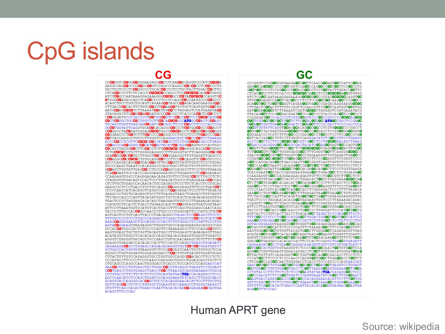
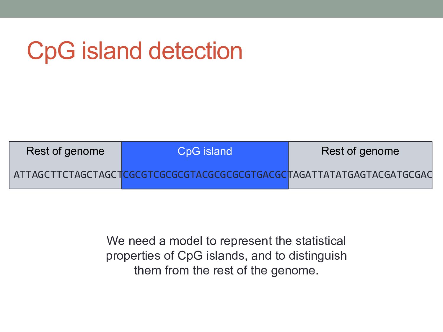
3. CpG islands • CpG site = location with a “C” directly followed by “G” • CpG sites are targets of DNA methylation • Addition of CH3 in C-nucleotides • Roles in gene regulation (typically silenced) • Mechanism of epigenetic memory • But… CpG sites have a tendency to get mutated • CG à TG • Therefore, “CG” dinucleotides are rare in vertebrate genomes • CpG islands: regions with many CpG sites • >200bp • GC content greater than usual • “CG” dinucleotides more common than rest of genome • Typically near gene promoters • Seem to be protected from DNA methylation
4. CpG islands CG GC Source: wikipedia Human APRT gene
5. Rest of genome Rest of genome CpG island CpG island detection ATTAGCTTCTAGCTAGCTCGCGTCGCGCGTACGCGCGCGTGACGCTAGATTATATGAGTACGATGCGAC We need a model to represent the statistical properties of CpG islands, and to distinguish them from the rest of the genome.
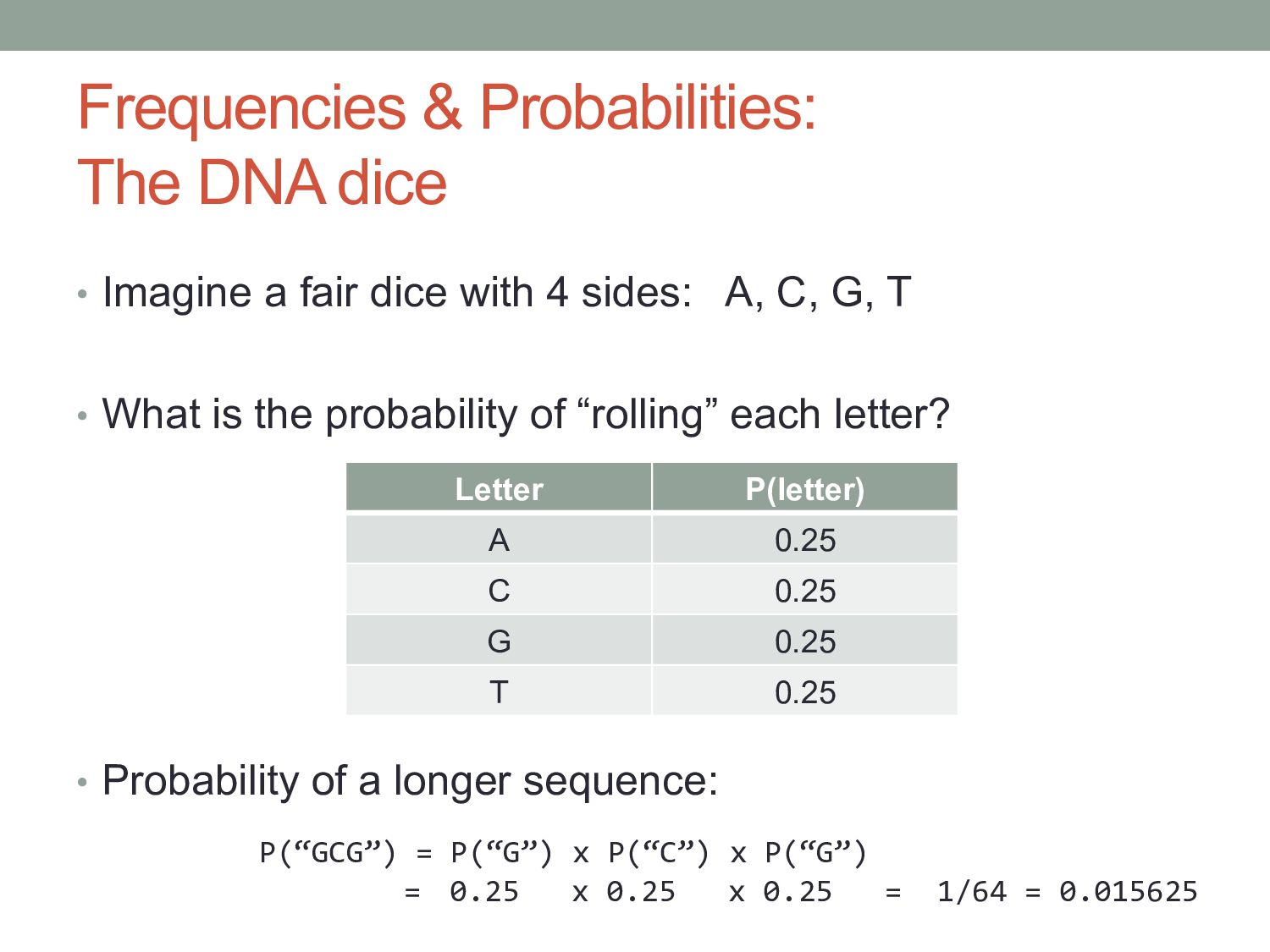
6. Frequencies & Probabilities: The DNA dice • Imagine a fair dice with 4 sides: A, C, G, T • What is the probability of “rolling” each letter? • Probability of a longer sequence: Letter P(letter) A 0.25 C 0.25 G 0.25 T 0.25 P(“GCG”) = P(“G”) x P(“C”) x P(“G”) = 0.25 x 0.25 x 0.25 = 1/64 = 0.015625
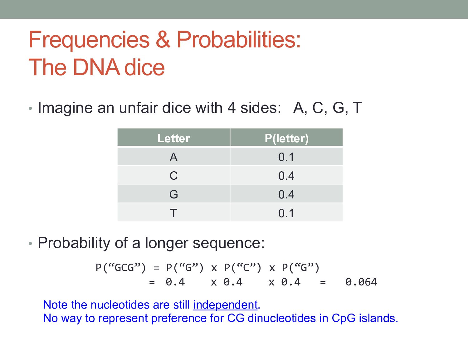
7. Frequencies & Probabilities: The DNA dice • Imagine an unfair dice with 4 sides: A, C, G, T • Probability of a longer sequence: Letter P(letter) A 0.1 C 0.4 G 0.4 T 0.1 P(“GCG”) = P(“G”) x P(“C”) x P(“G”) = 0.4 x 0.4 x 0.4 = 0.064 Note the nucleotides are still independent. No way to represent preference for CG dinucleotides in CpG islands.
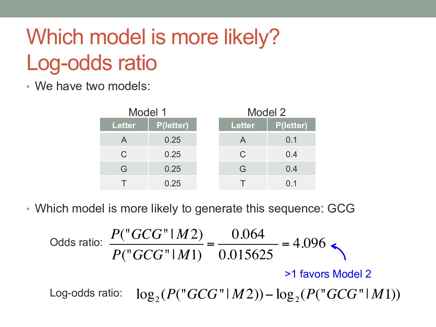
8. Which model is more likely? Log-odds ratio • We have two models: • Which model is more likely to generate this sequence: GCG Letter P(letter) A 0.25 C 0.25 G 0.25 T 0.25 Letter P(letter) A 0.1 C 0.4 G 0.4 T 0.1 Model 1 Model 2 Odds ratio: P("GCG"| M2) P("GCG"| M1) = 0.064 0.015625 = 4.096 >1 favors Model 2 Log-odds ratio: log 2 (P("GCG"| M2))− log 2 (P("GCG"| M1))
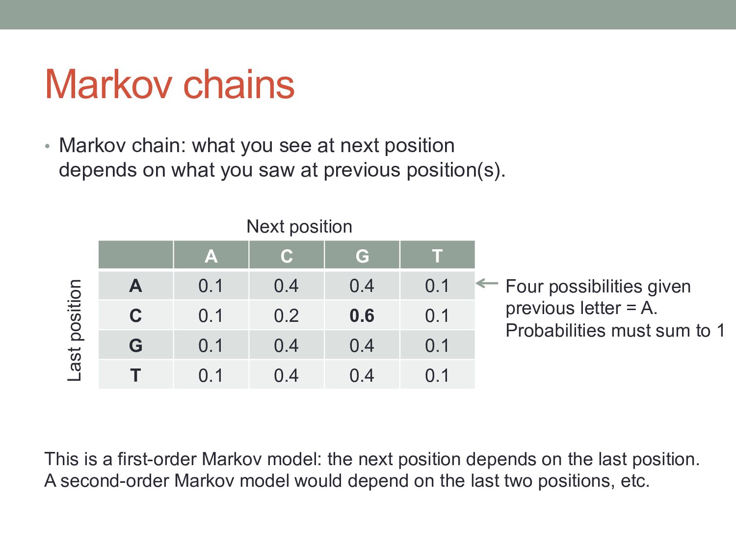
9. Markov chains • Markov chain: what you see at next position depends on what you saw at previous position(s). Four possibilities given previous letter = A. Probabilities must sum to 1 A C G T A 0.1 0.4 0.4 0.1 C 0.1 0.2 0.6 0.1 G 0.1 0.4 0.4 0.1 T 0.1 0.4 0.4 0.1 Next position Last position This is a first-order Markov model: the next position depends on the last position. A second-order Markov model would depend on the last two positions, etc.
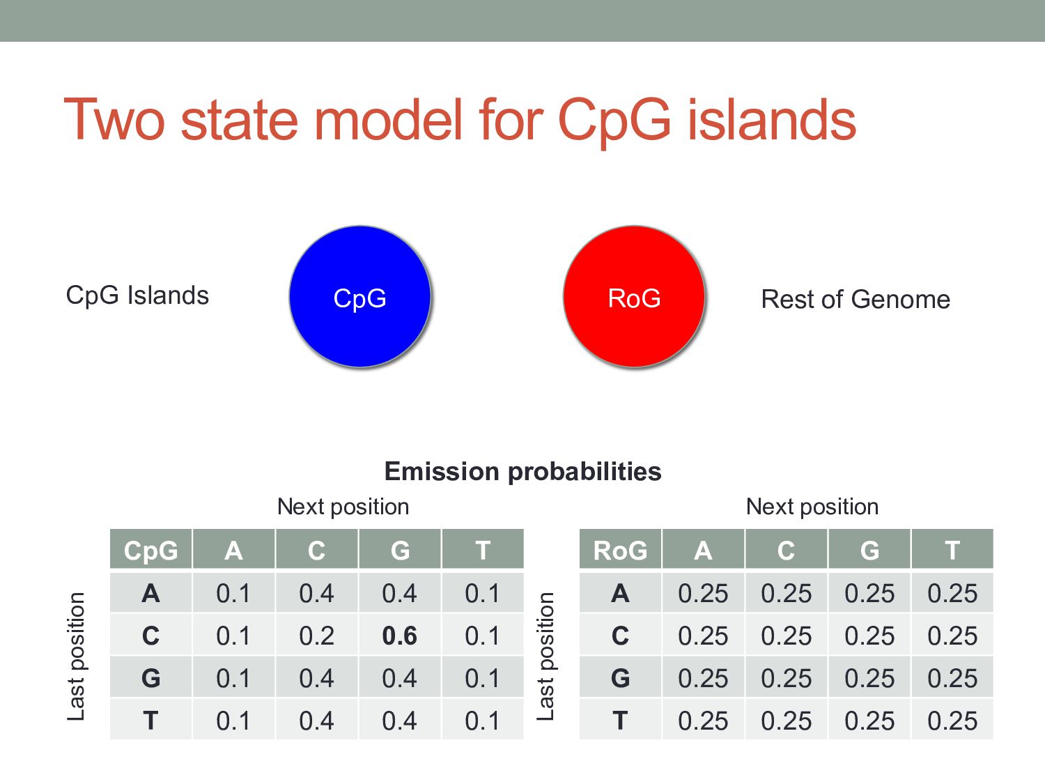
10. Two state model for CpG islands CpG A C G T A 0.1 0.4 0.4 0.1 C 0.1 0.2 0.6 0.1 G 0.1 0.4 0.4 0.1 T 0.1 0.4 0.4 0.1 Next position Last position RoG A C G T A 0.25 0.25 0.25 0.25 C 0.25 0.25 0.25 0.25 G 0.25 0.25 0.25 0.25 T 0.25 0.25 0.25 0.25 Next position Last position CpG RoG Rest of Genome CpG Islands Emission probabilities
11. Two state model for CpG islands CpG RoG 0.9 0.1 0.2 0.8 CpG RoG CpG 0.8 0.2 RoG 0.1 0.9 Next state Last state Transition probabilities “Graphical model” Note this is also a Markov chain
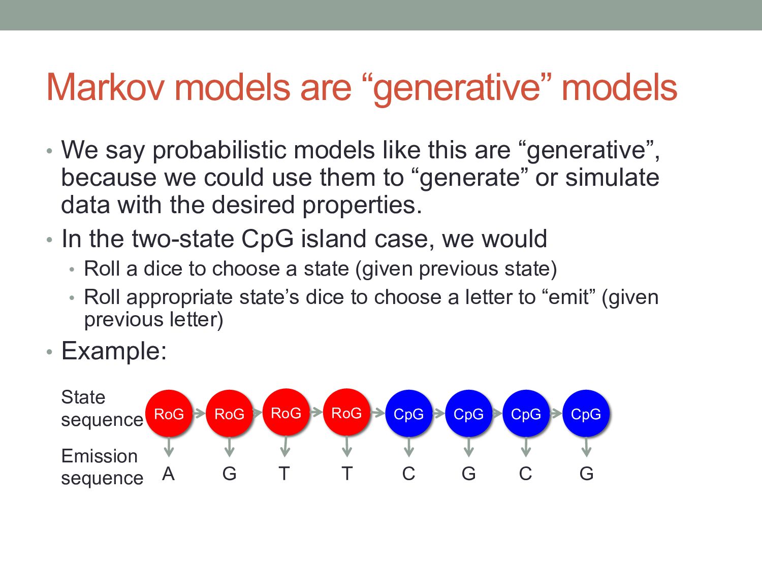
12. Markov models are “generative” models • We say probabilistic models like this are “generative”, because we could use them to “generate” or simulate data with the desired properties. • In the two-state CpG island case, we would • Roll a dice to choose a state (given previous state) • Roll appropriate state’s dice to choose a letter to “emit” (given previous letter) • Example: RoG A G T T C G C G RoG RoG RoG CpG CpG CpG CpG State sequence Emission sequence
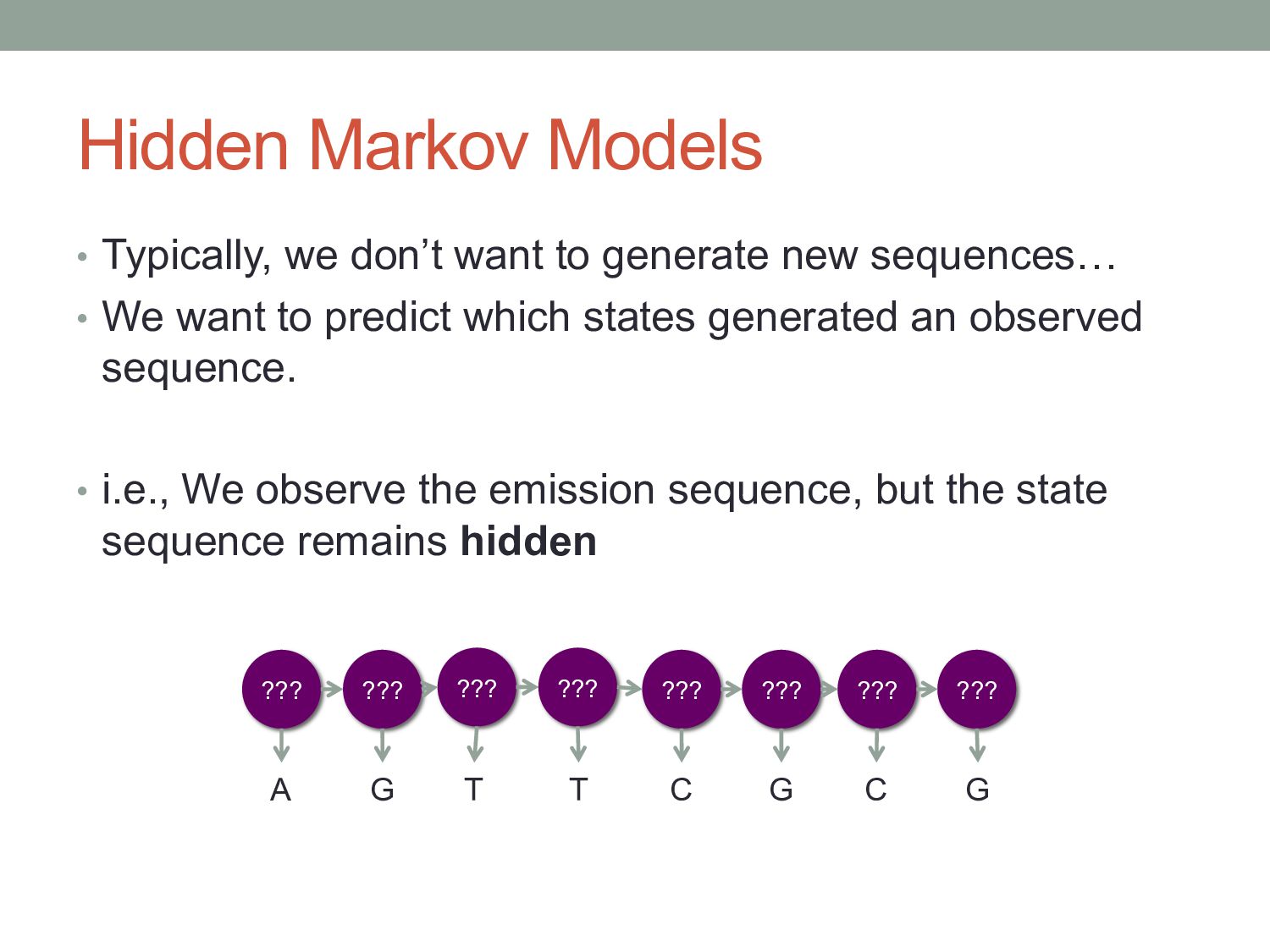
13. Hidden Markov Models • Typically, we don’t want to generate new sequences… • We want to predict which states generated an observed sequence. • i.e., We observe the emission sequence, but the state sequence remains hidden ??? A G T T C G C G ??? ??? ??? ??? ??? ??? ???
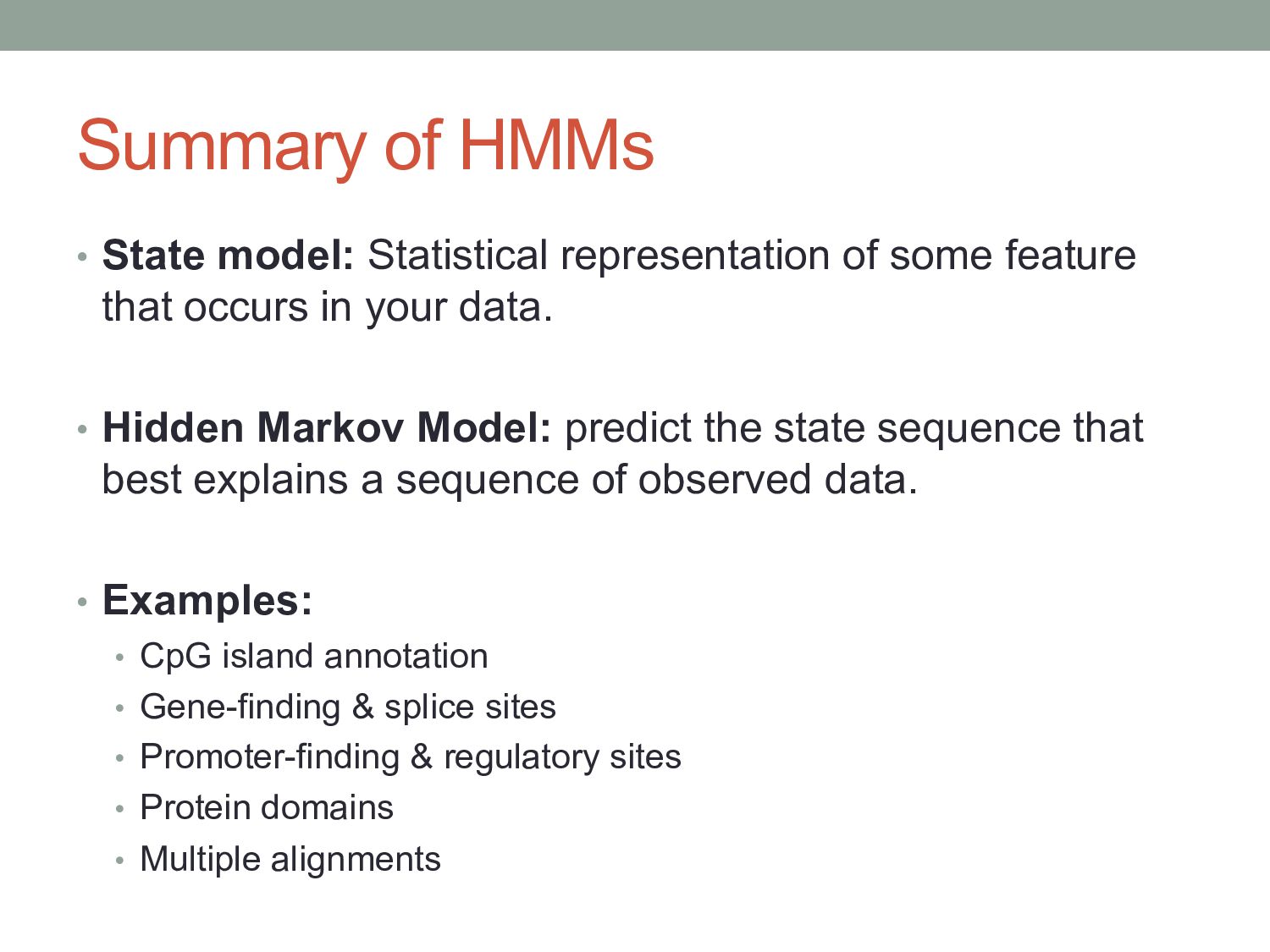
14. Summary of HMMs • State model: Statistical representation of some feature that occurs in your data. • Hidden Markov Model: predict the state sequence that best explains a sequence of observed data. • Examples: • CpG island annotation • Gene-finding & splice sites • Promoter-finding & regulatory sites • Protein domains • Multiple alignments
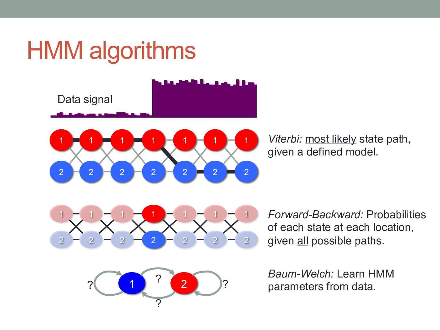
15. HMM algorithms 1 1 2 2 1 2 1 2 1 2 1 2 1 2 1 1 2 2 1 2 1 2 1 2 1 2 1 2 Viterbi: most likely state path, given a defined model. Forward-Backward: Probabilities of each state at each location, given all possible paths. 1 2 ? ? ? ? Baum-Welch: Learn HMM parameters from data. Data signal
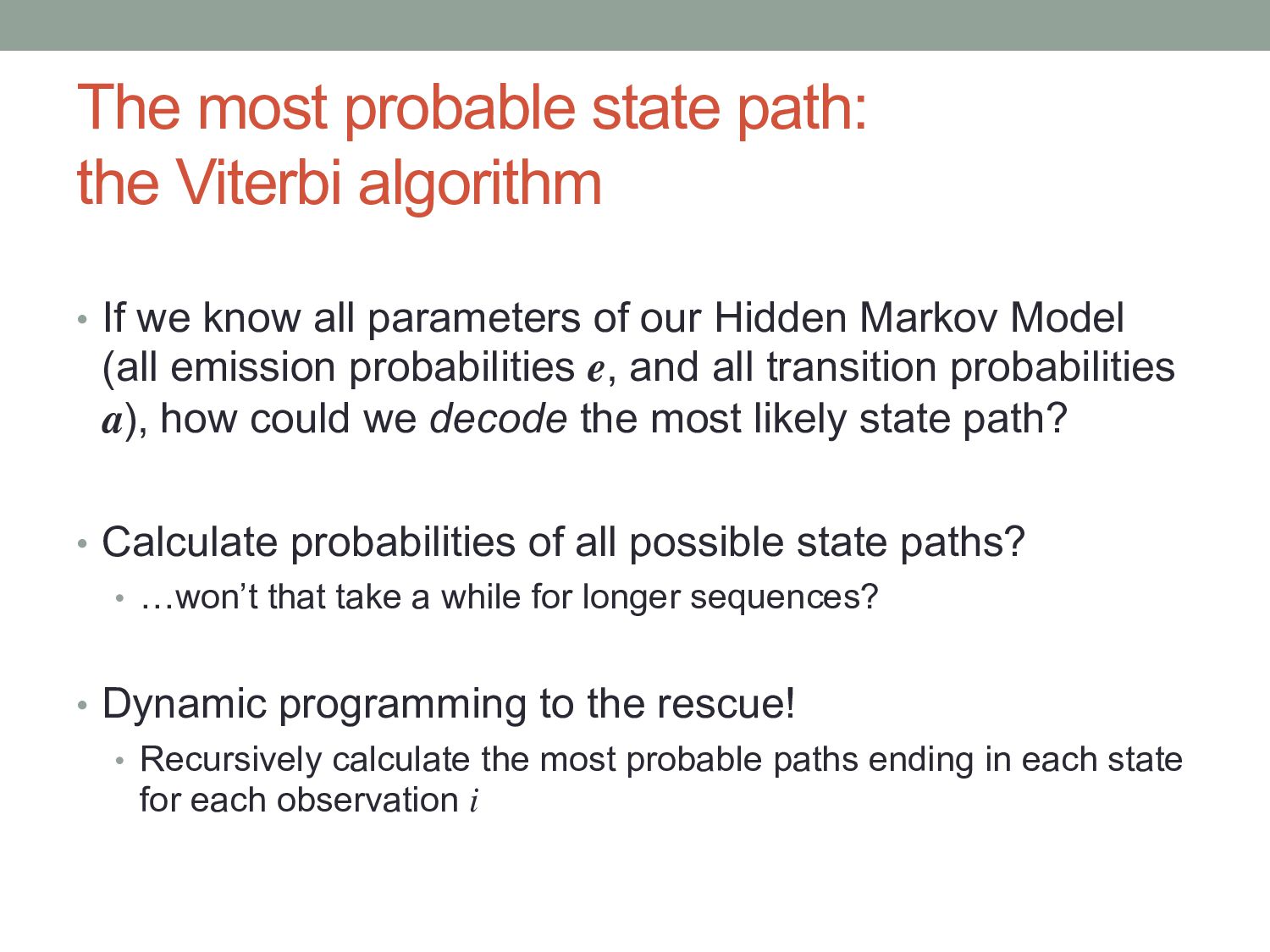
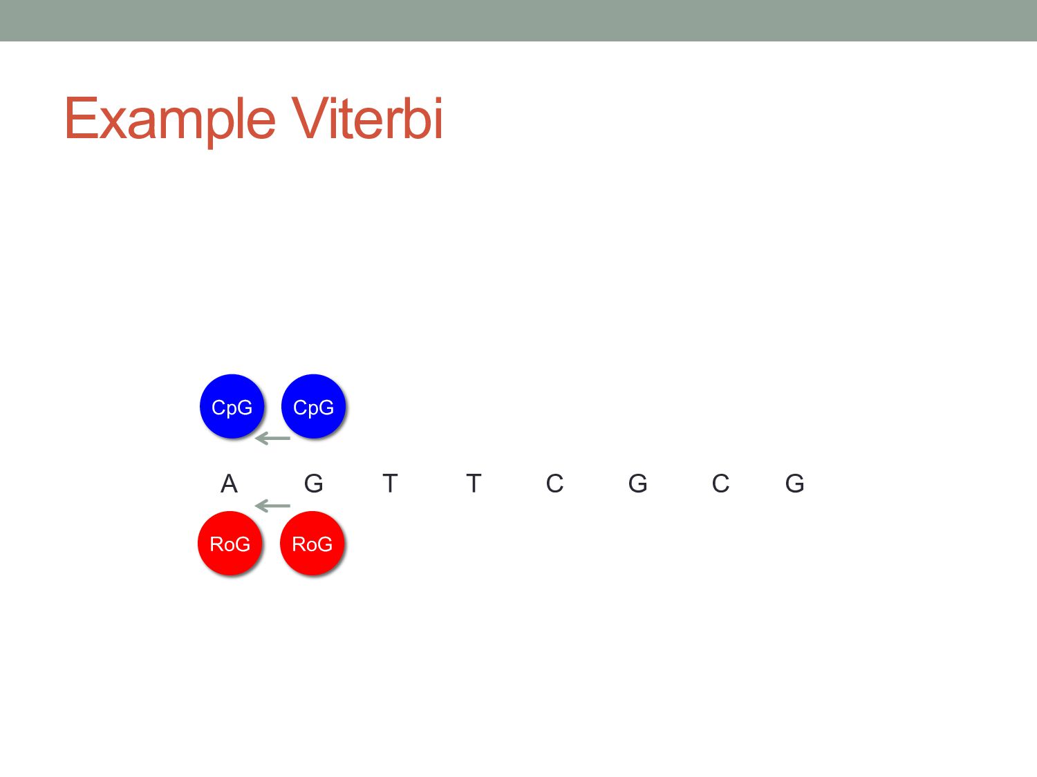
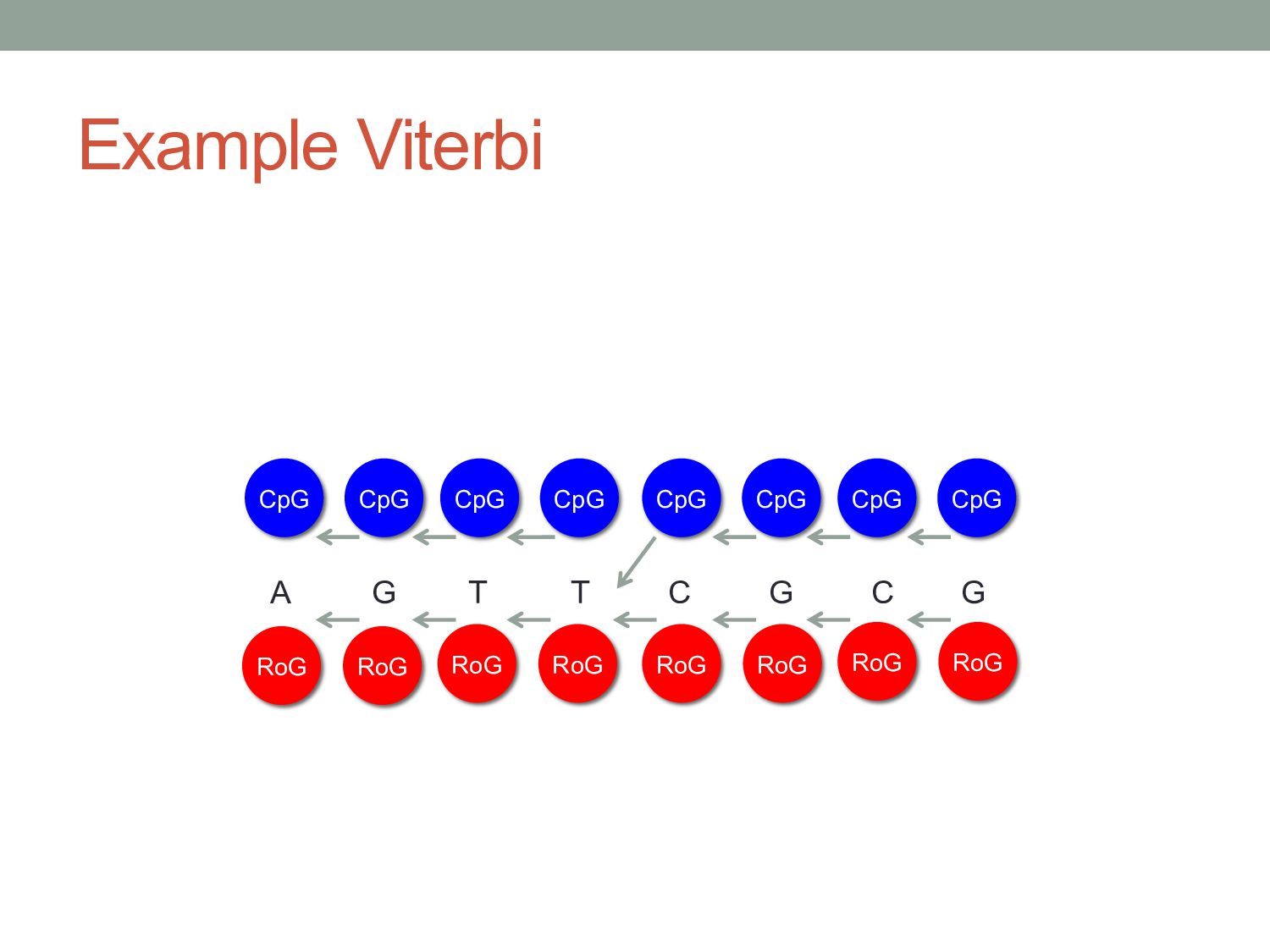
16. The most probable state path: the Viterbi algorithm • If we know all parameters of our Hidden Markov Model (all emission probabilities e, and all transition probabilities a), how could we decode the most likely state path? • Calculate probabilities of all possible state paths? • …won’t that take a while for longer sequences? • Dynamic programming to the rescue! • Recursively calculate the most probable paths ending in each state for each observation i
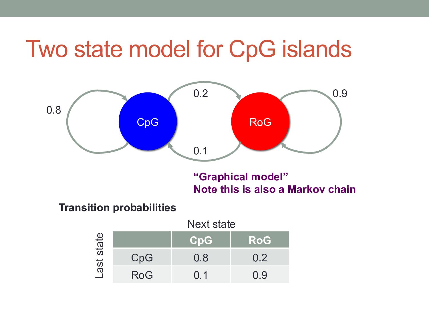
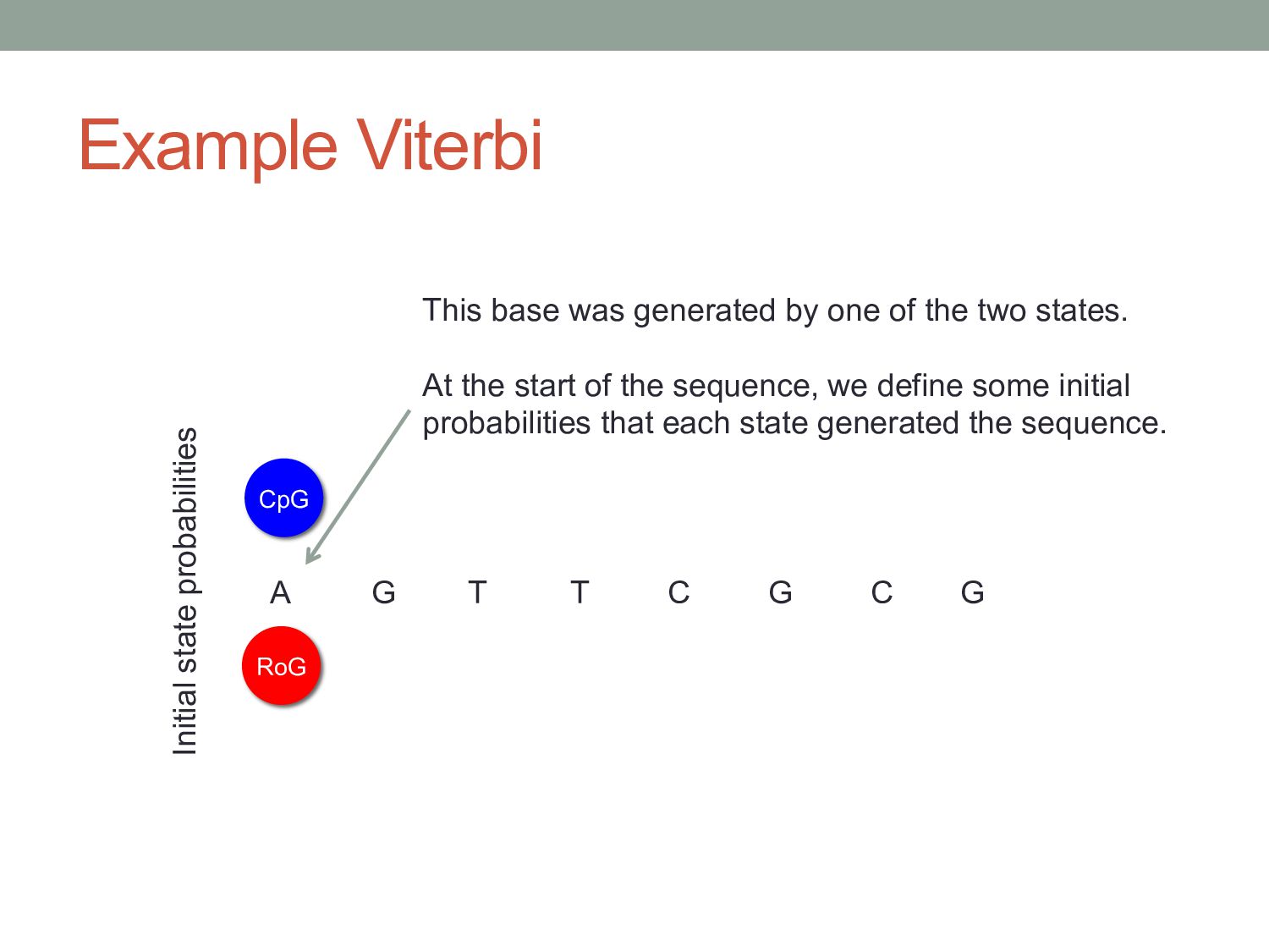
17. Example Viterbi RoG A G T T C G C G CpG Initial state probabilities This base was generated by one of the two states. At the start of the sequence, we define some initial probabilities that each state generated the sequence.
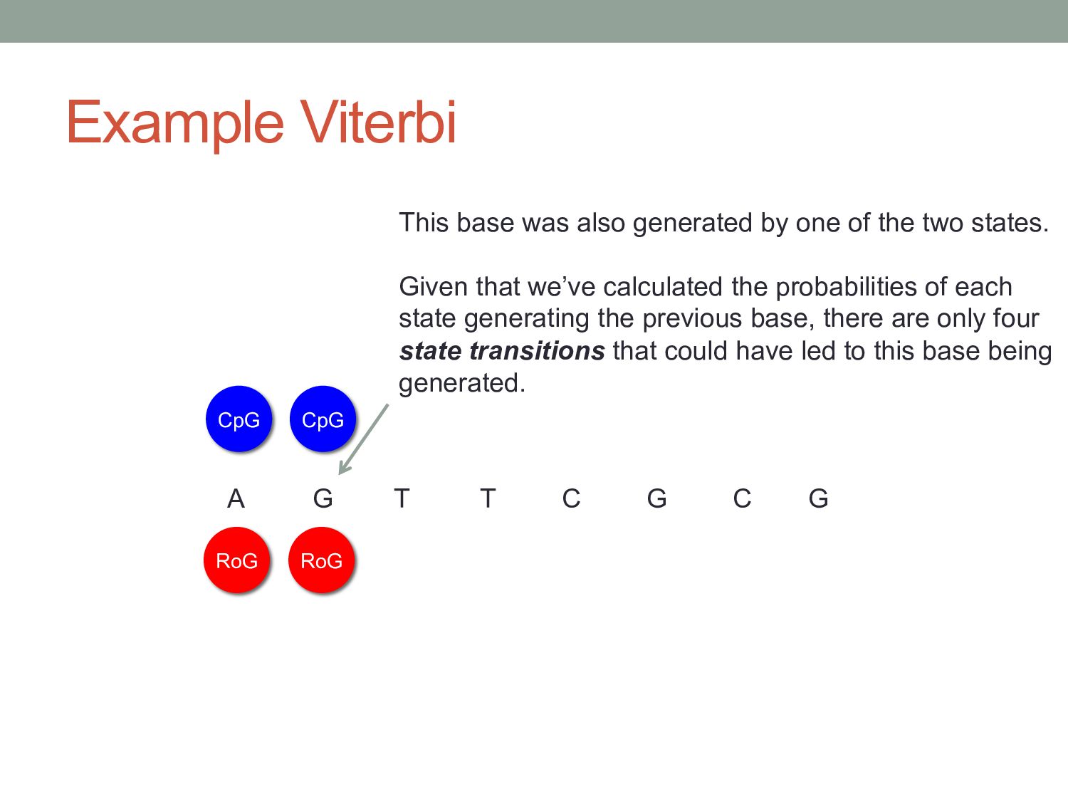
18. Example Viterbi RoG A G T T C G C G RoG CpG CpG This base was also generated by one of the two states. Given that we’ve calculated the probabilities of each state generating the previous base, there are only four state transitions that could have led to this base being generated.
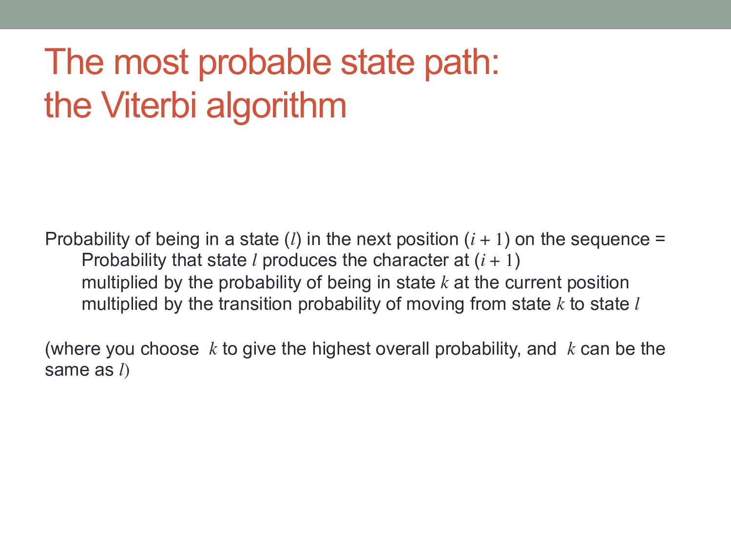
19. The most probable state path: the Viterbi algorithm Probability of being in a state (l) in the next position (i + 1) on the sequence = Probability that state l produces the character at (i + 1) multiplied by the probability of being in state k at the current position multiplied by the transition probability of moving from state k to state l (where you choose k to give the highest overall probability, and k can be the same as l)
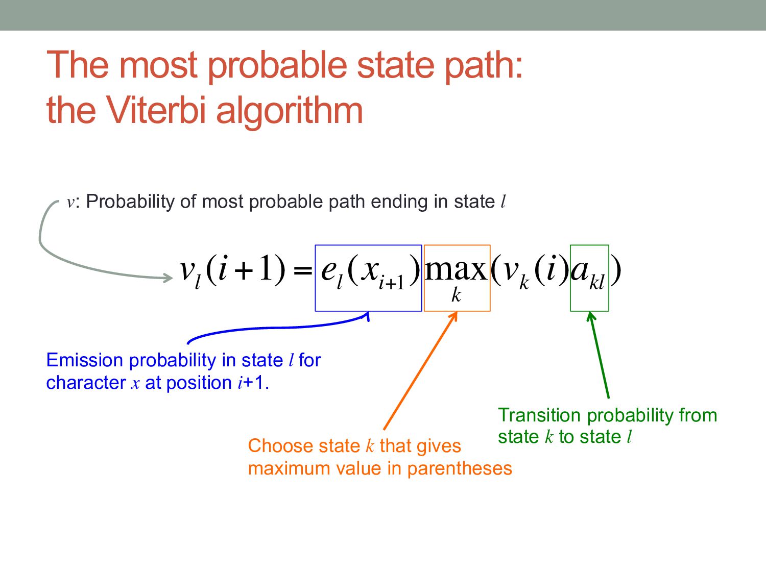
20. The most probable state path: the Viterbi algorithm v l (i+1) = e l (x i+1 )max k (v k (i)a kl ) v: Probability of most probable path ending in state l Emission probability in state l for character x at position i+1. Transition probability from state k to state l Choose state k that gives maximum value in parentheses
21. Example Viterbi RoG A G T T C G C G RoG CpG CpG
22. Example Viterbi RoG A G T T C G C G RoG RoG RoG CpG CpG CpG CpG RoG RoG RoG RoG CpG CpG CpG CpG
23. Example Viterbi RoG A G T T C G C G RoG RoG RoG RoG RoG RoG RoG CpG CpG CpG CpG CpG CpG CpG CpG Final traceback:
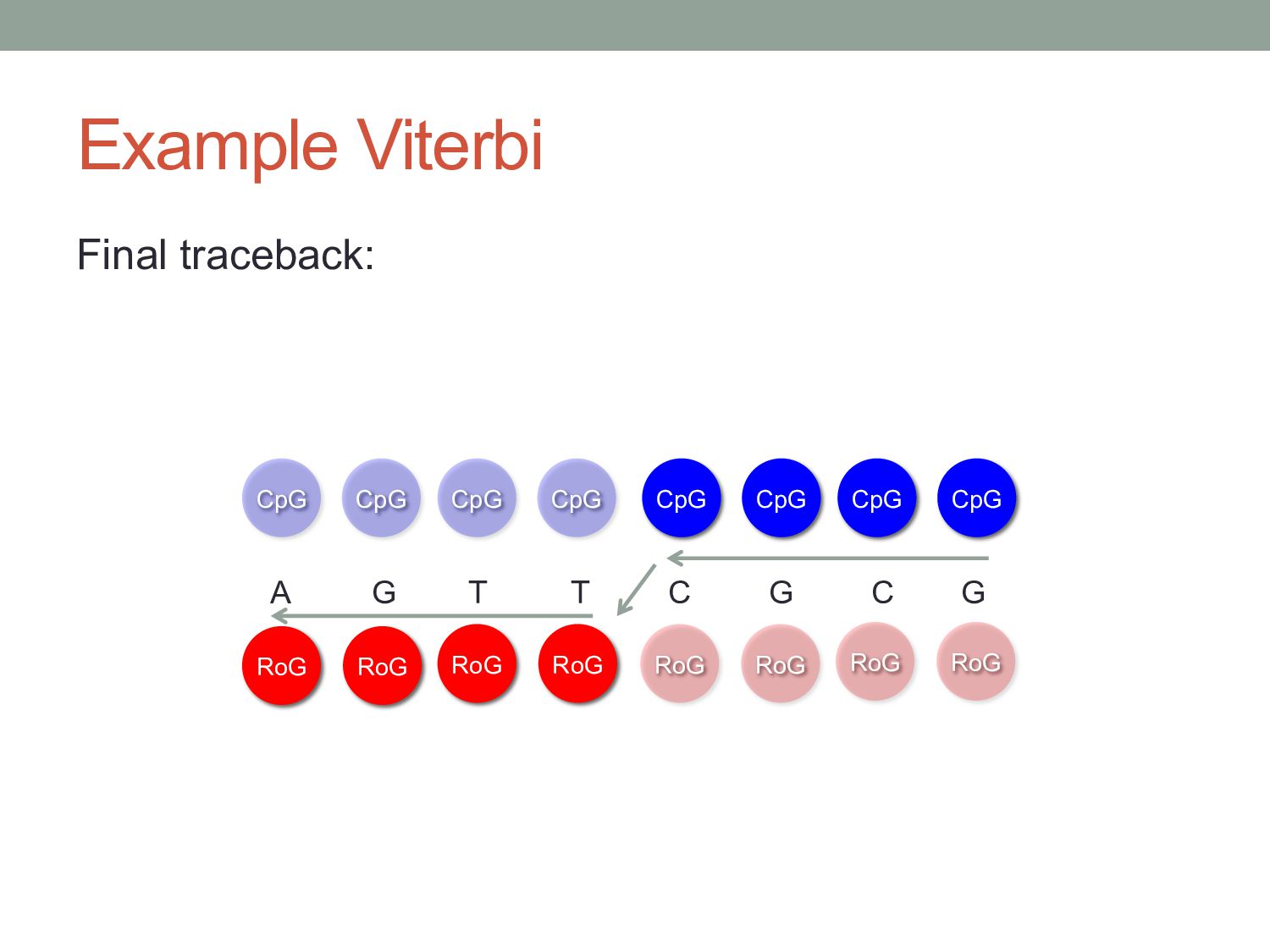
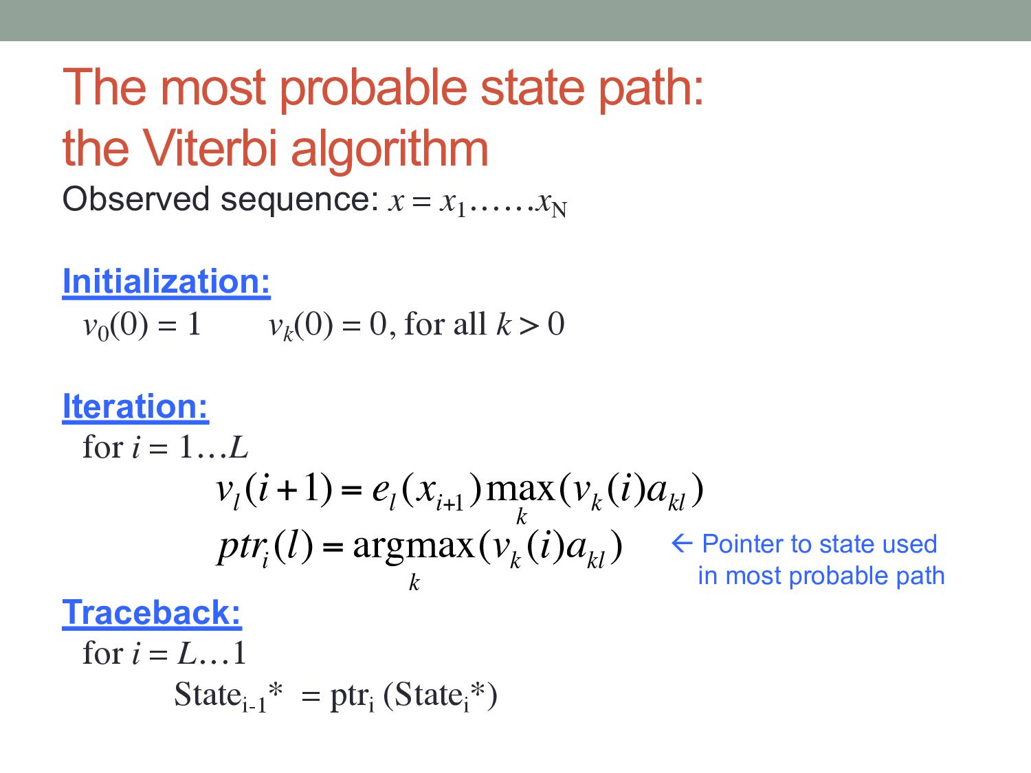
24. The most probable state path: the Viterbi algorithm Observed sequence: x = x1 ……xN Initialization: v0 (0) = 1 vk (0) = 0, for all k > 0 Iteration: for i = 1…L Traceback: for i = L…1 Statei-1 * = ptri (Statei *) v l (i+1) = e l (x i+1 )max k (v k (i)a kl ) ptr i (l) = argmax k (v k (i)a kl ) ß Pointer to state used in most probable path
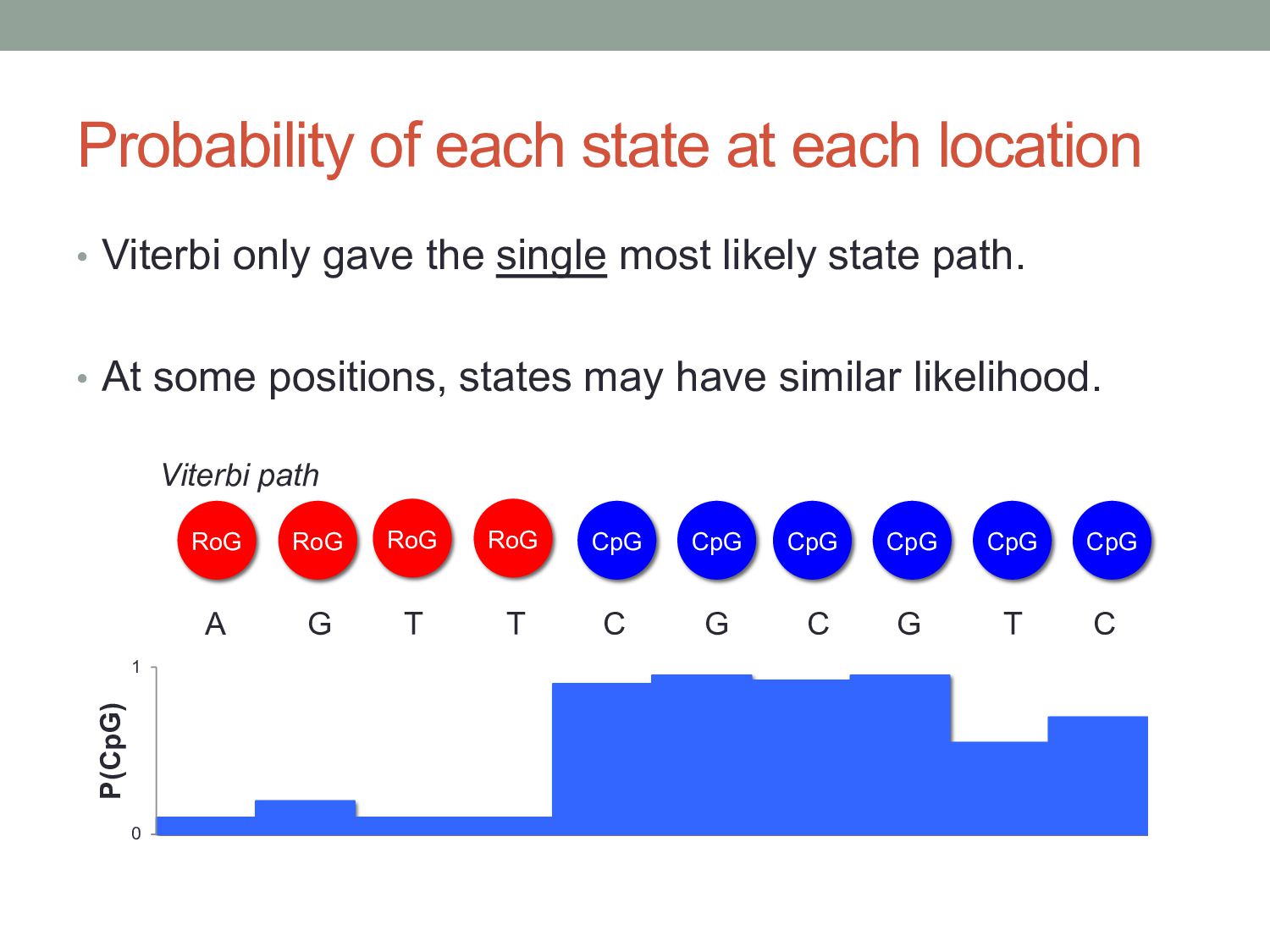
25. Probability of each state at each location • Viterbi only gave the single most likely state path. • At some positions, states may have similar likelihood. RoG A G T T C G C G RoG RoG RoG CpG CpG CpG CpG CpG CpG T C Viterbi path 0 1 P(CpG)
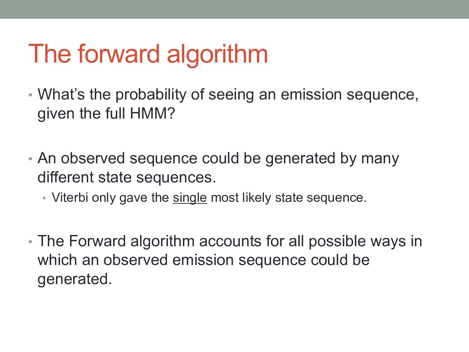
26. The forward algorithm • What’s the probability of seeing an emission sequence, given the full HMM? • An observed sequence could be generated by many different state sequences. • Viterbi only gave the single most likely state sequence. • The Forward algorithm accounts for all possible ways in which an observed emission sequence could be generated.
27. Probability of a sequence: the Forward algorithm Observed sequence: x = x1 ……xN Initialization: f0 (0) = 1 fk (0) = 0, for all k > 0 Iteration: for i = 1…L Termination: P(x) = Σk fk (N) ak0 f l (i+1) = e l (x i+1 ) ( f k (i)a kl ) k ∑ Sum instead of choosing max
28. Probability of a sequence: the Backward algorithm Observed sequence: x = x1 ……xN Initialization: bk (L) = ak0 , for all k Iteration: for i = L…1 b k (i) = b l (i+1)a kl e l (x i+1 ) l ∑ Sum (as in Forward algorithm)
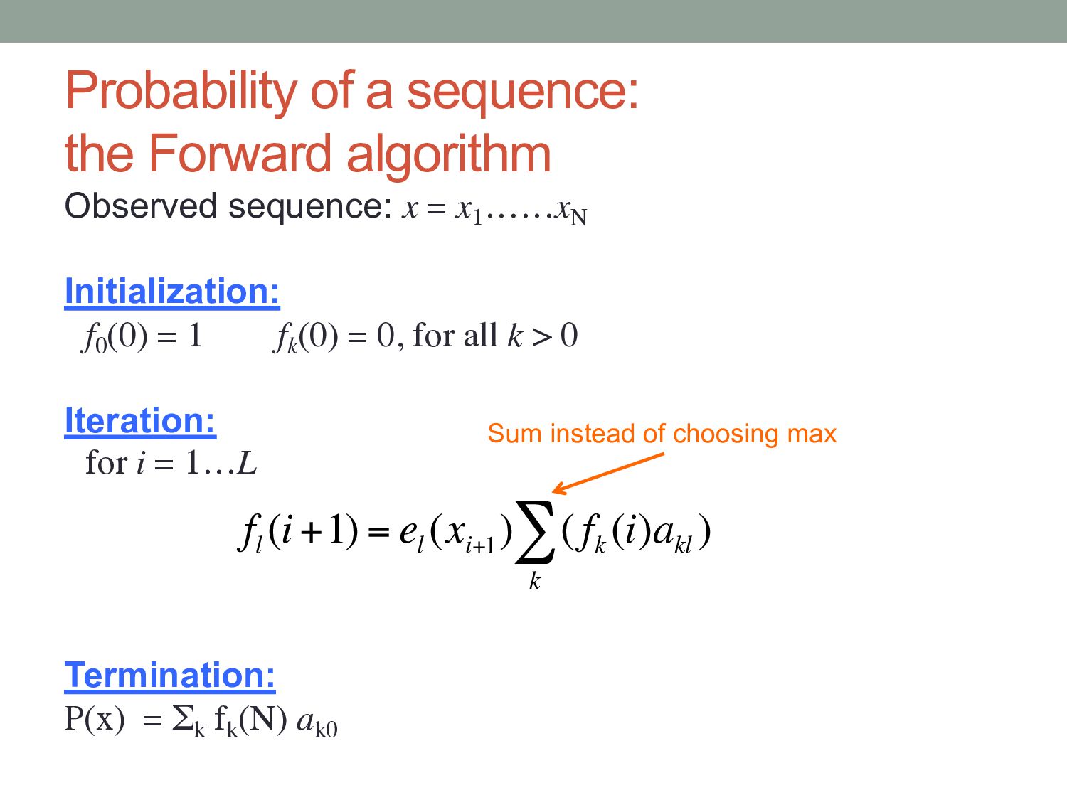
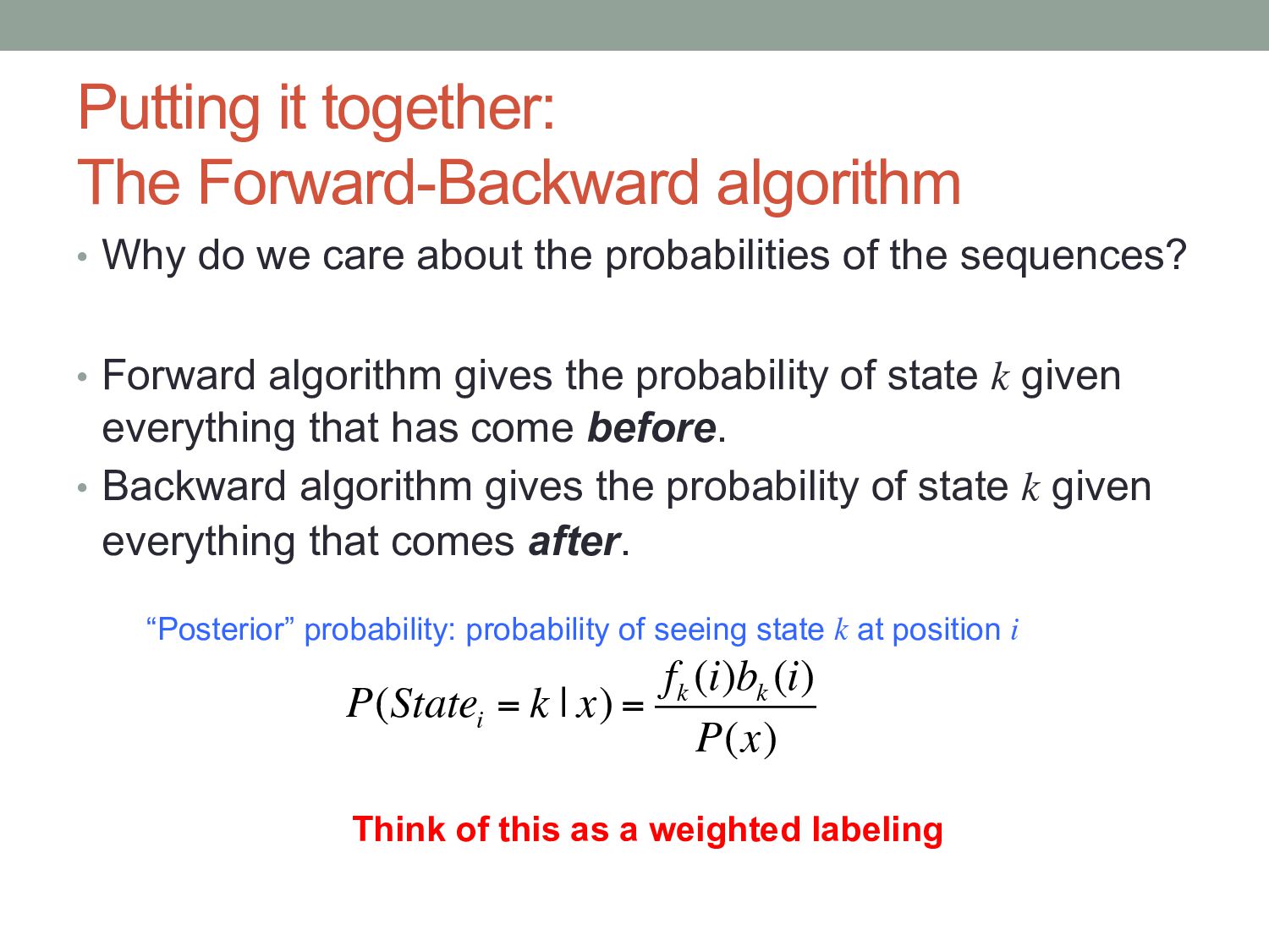
29. Putting it together: The Forward-Backward algorithm • Why do we care about the probabilities of the sequences? • Forward algorithm gives the probability of state k given everything that has come before. • Backward algorithm gives the probability of state k given everything that comes after. P(State i = k | x) = f k (i)b k (i) P(x) “Posterior” probability: probability of seeing state k at position i Think of this as a weighted labeling
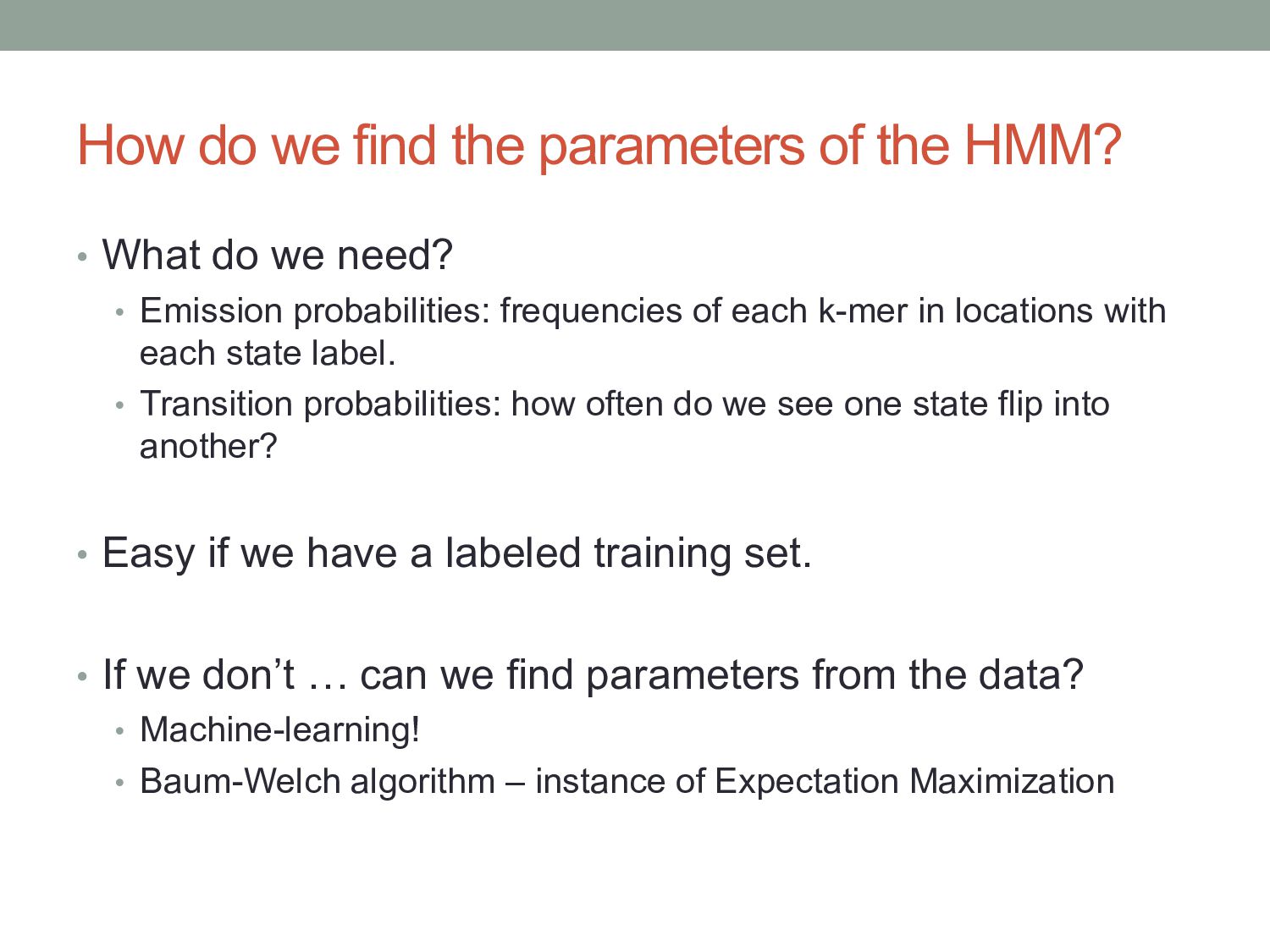
30. How do we find the parameters of the HMM? • What do we need? • Emission probabilities: frequencies of each k-mer in locations with each state label. • Transition probabilities: how often do we see one state flip into another? • Easy if we have a labeled training set. • If we don’t … can we find parameters from the data? • Machine-learning! • Baum-Welch algorithm – instance of Expectation Maximization
31. Baum-Welch: general idea • Start with some HMM parameters • Assign state labels to a sequence using the current HMM • Update the HMM parameters using the current labels
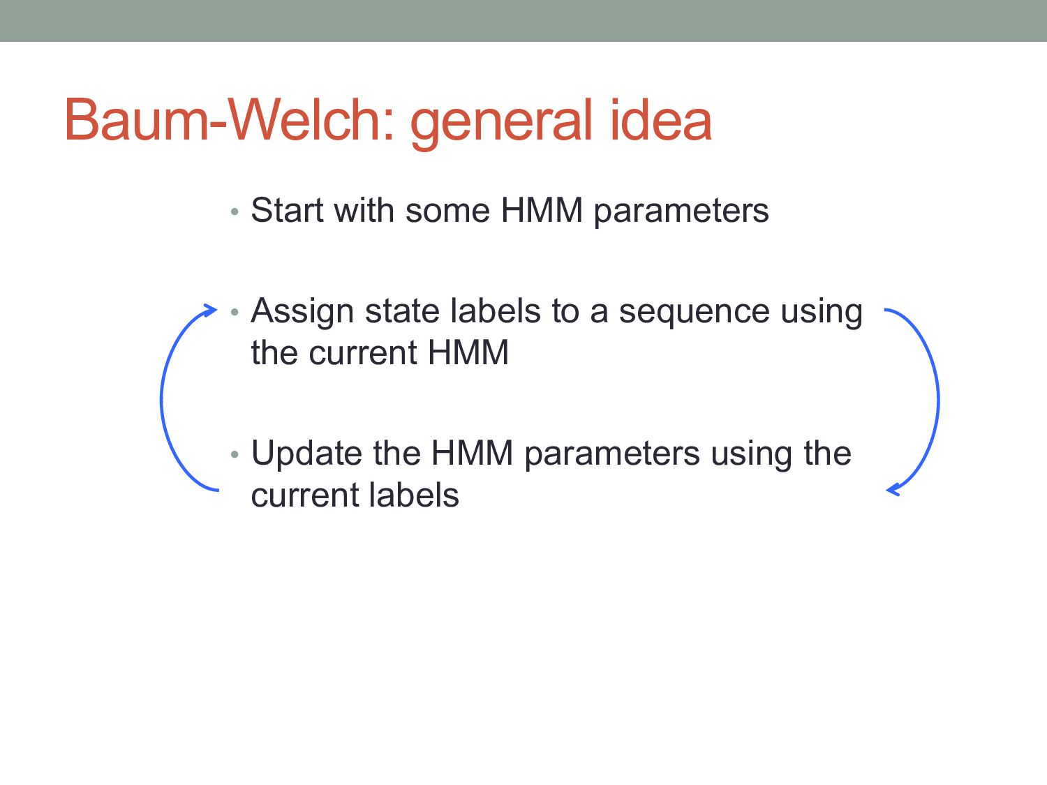
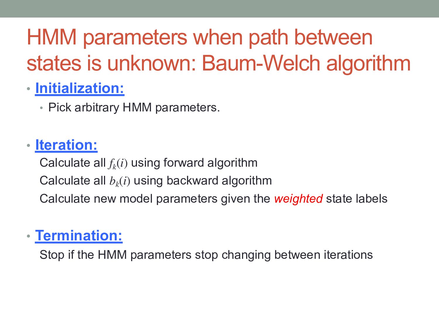
32. HMM parameters when path between states is unknown: Baum-Welch algorithm • Initialization: • Pick arbitrary HMM parameters. • Iteration: Calculate all fk (i) using forward algorithm Calculate all bk (i) using backward algorithm Calculate new model parameters given the weighted state labels • Termination: Stop if the HMM parameters stop changing between iterations
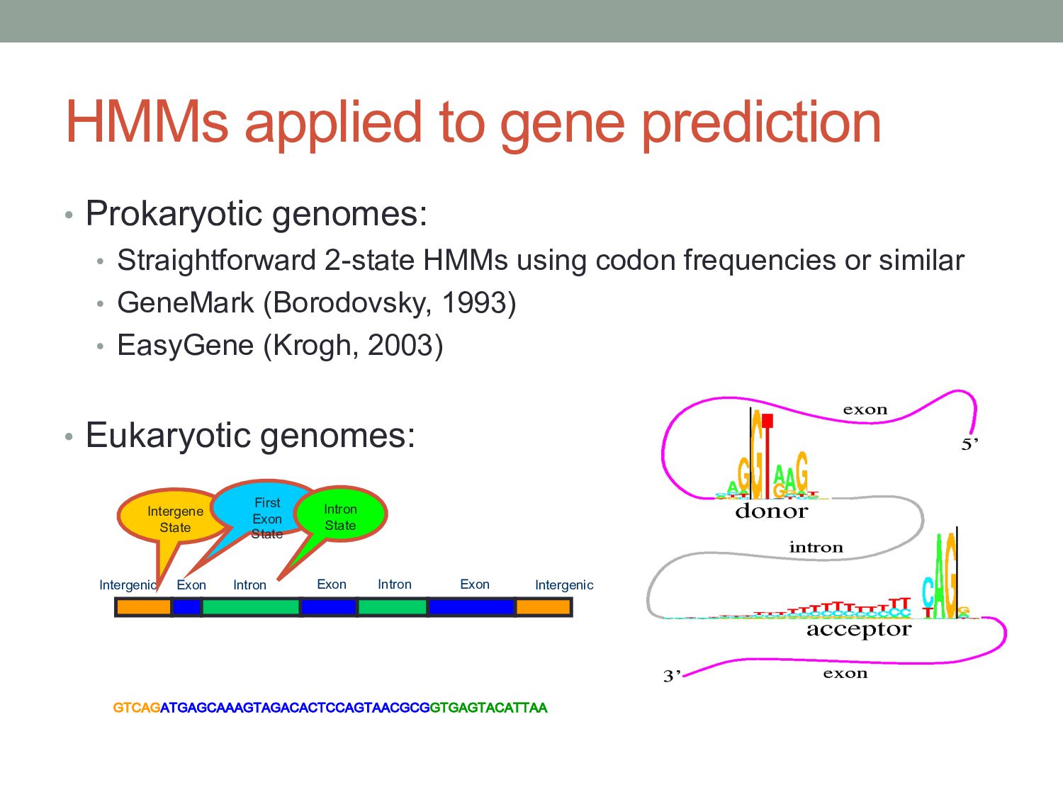
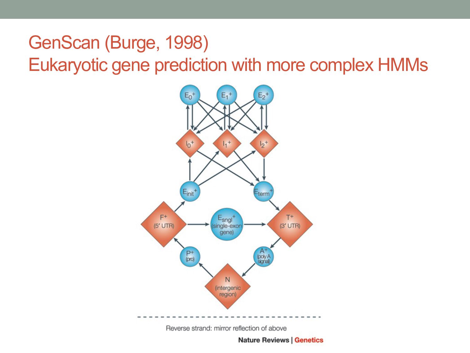
33. HMMs applied to gene prediction • Prokaryotic genomes: • Straightforward 2-state HMMs using codon frequencies or similar • GeneMark (Borodovsky, 1993) • EasyGene (Krogh, 2003) • Eukaryotic genomes: !"#$!$"!$!#$$$!"$!$#$#"##$!"$$#!#!!"!$!"$#$""$$ %&'( %&'( %&'( )(*+'( )(*+'( )(*,+-,(./ )(*,+-,(./ Intergene State First Exon State Intron State
34. GenScan (Burge, 1998) Eukaryotic gene prediction with more complex HMMs
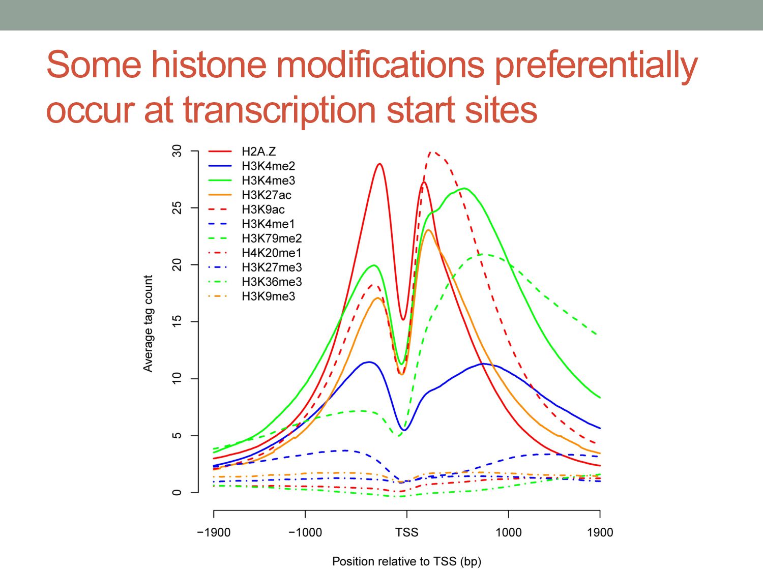
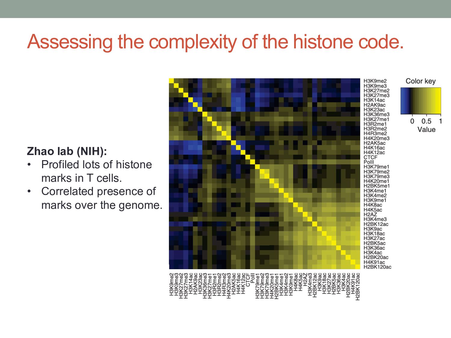
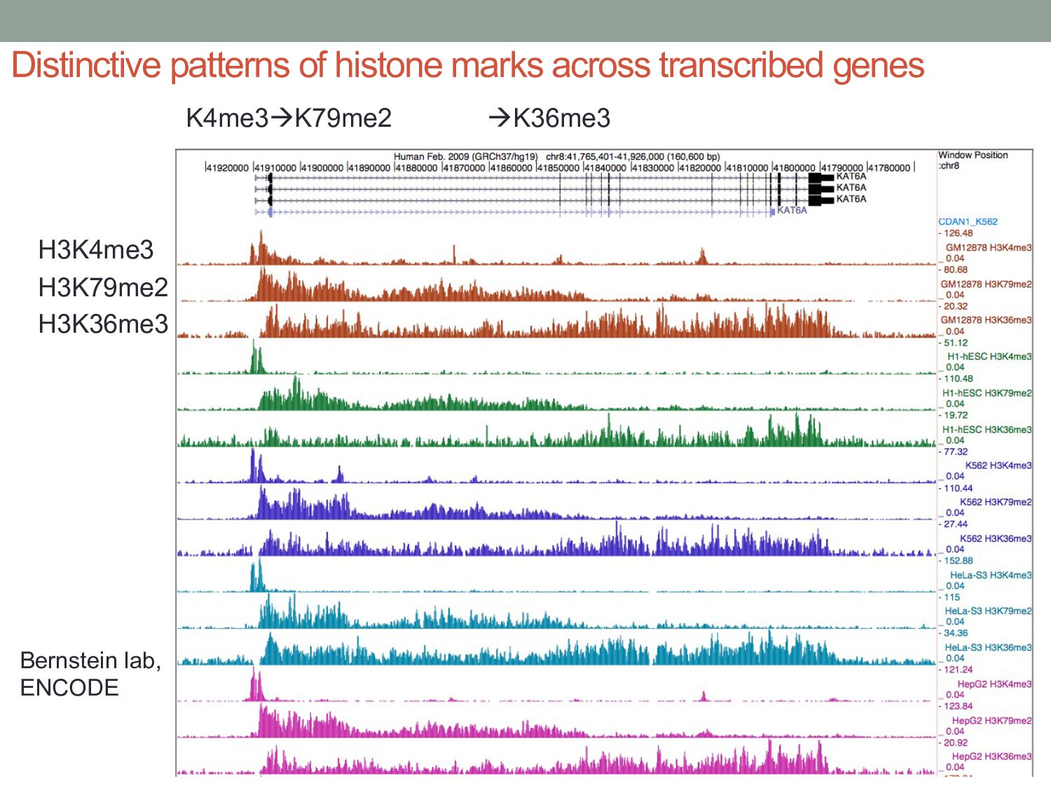
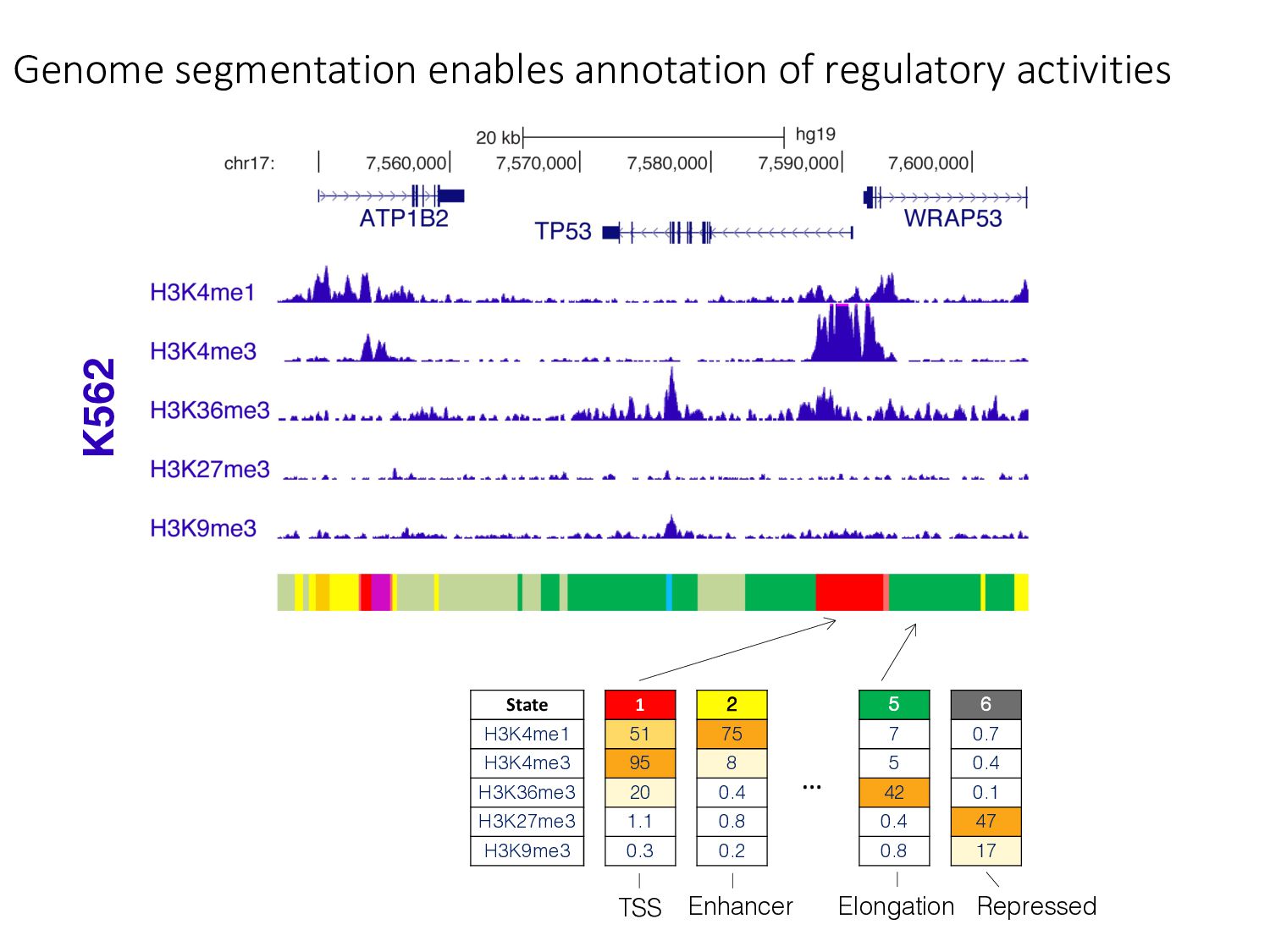
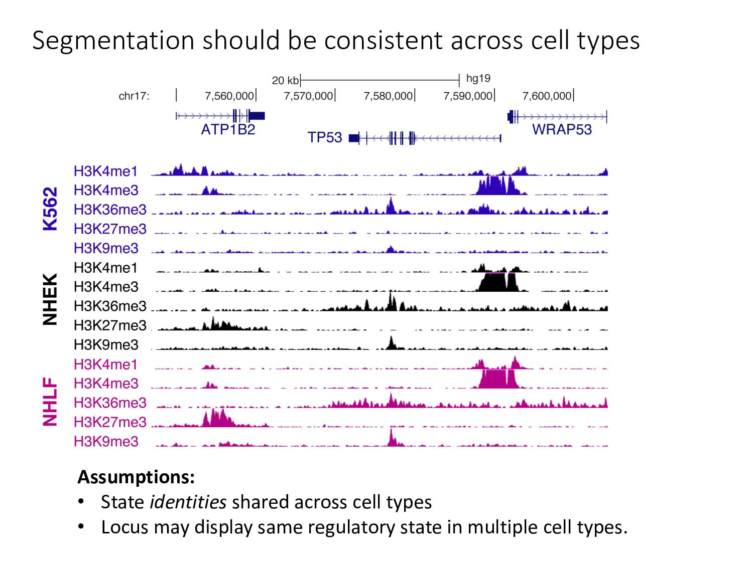
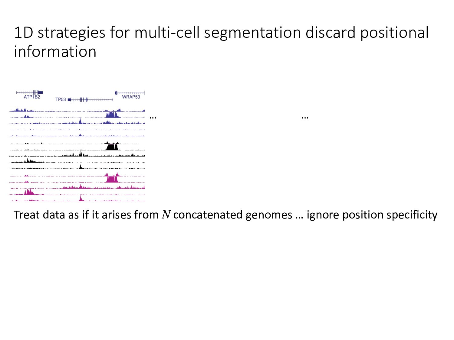
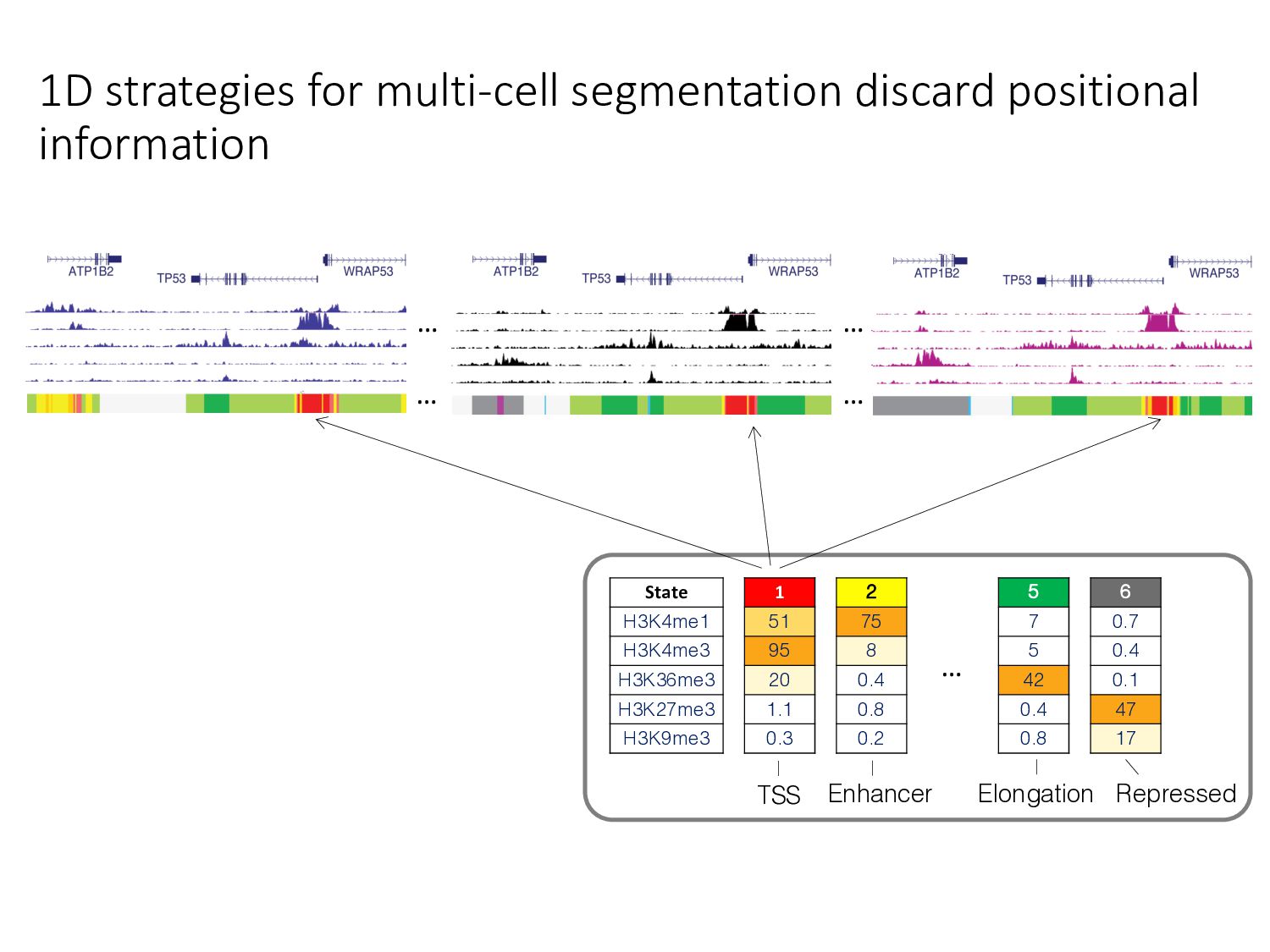
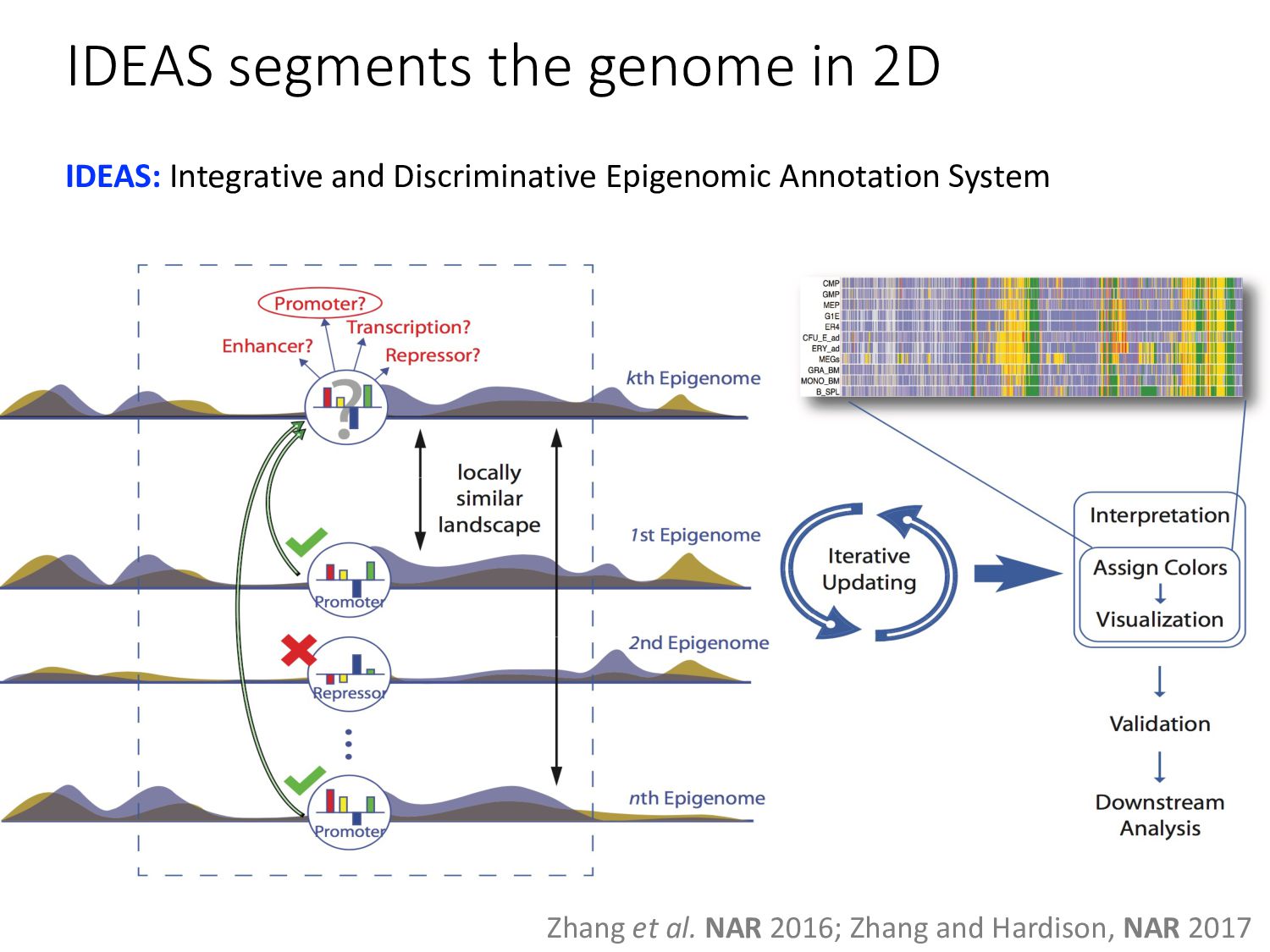
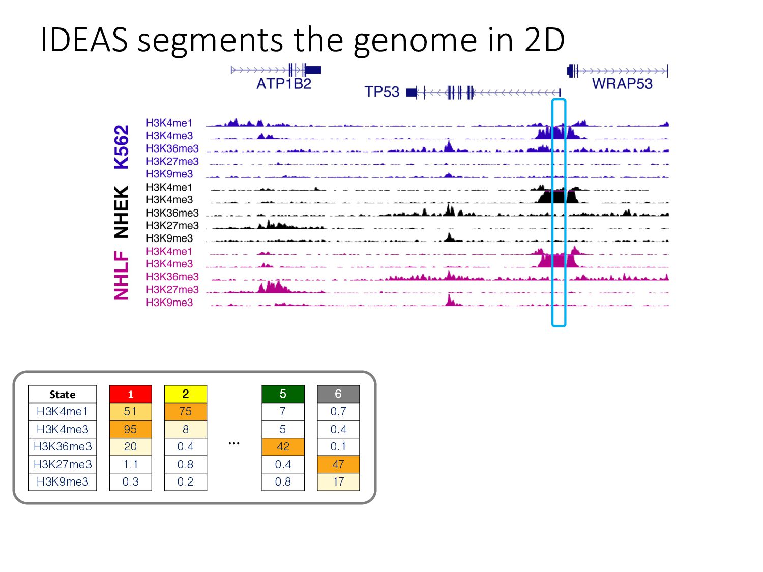
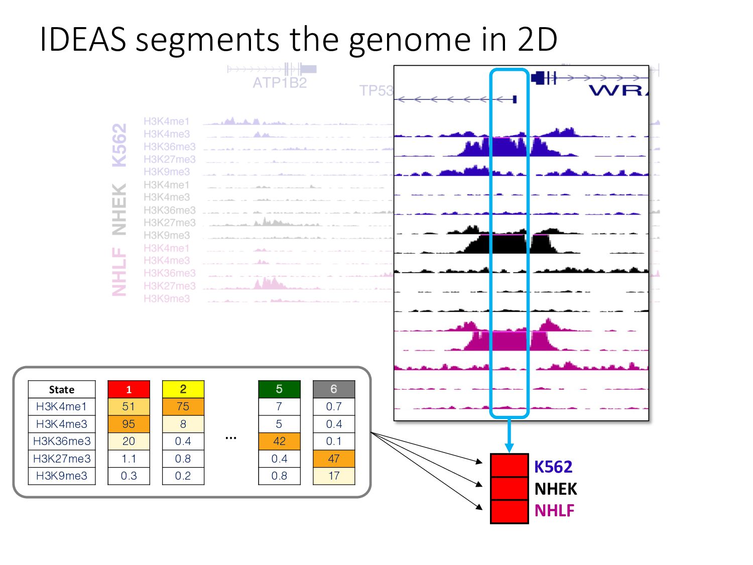
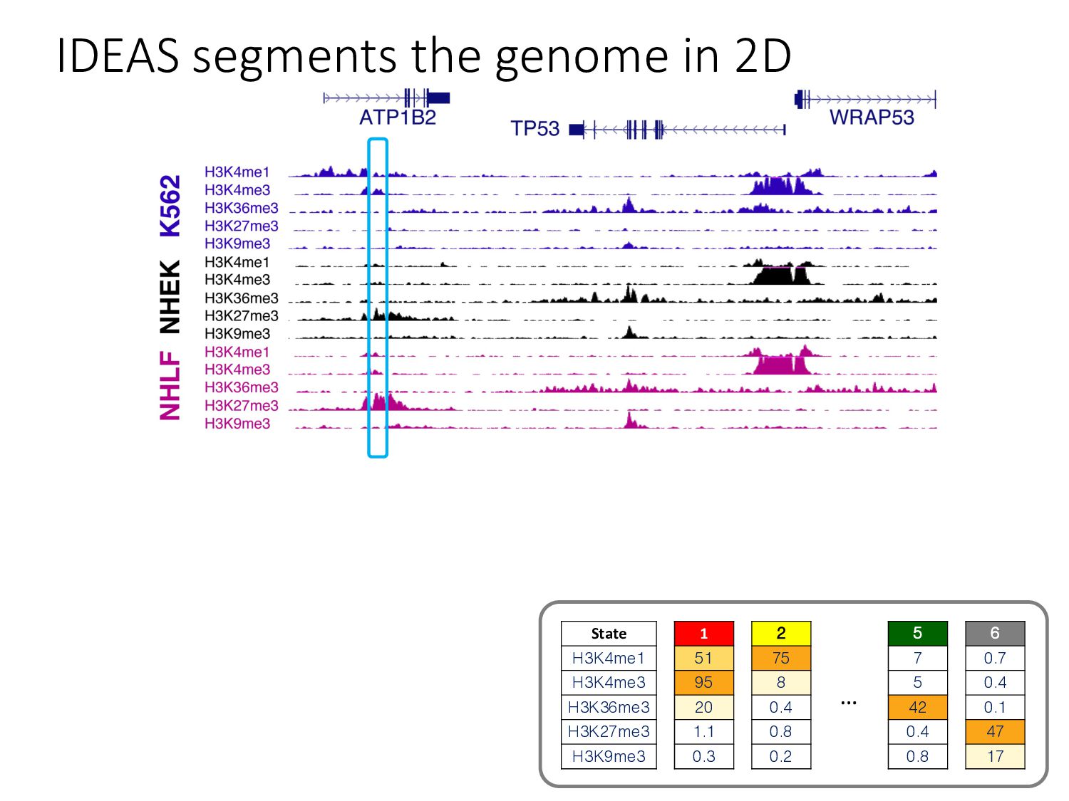
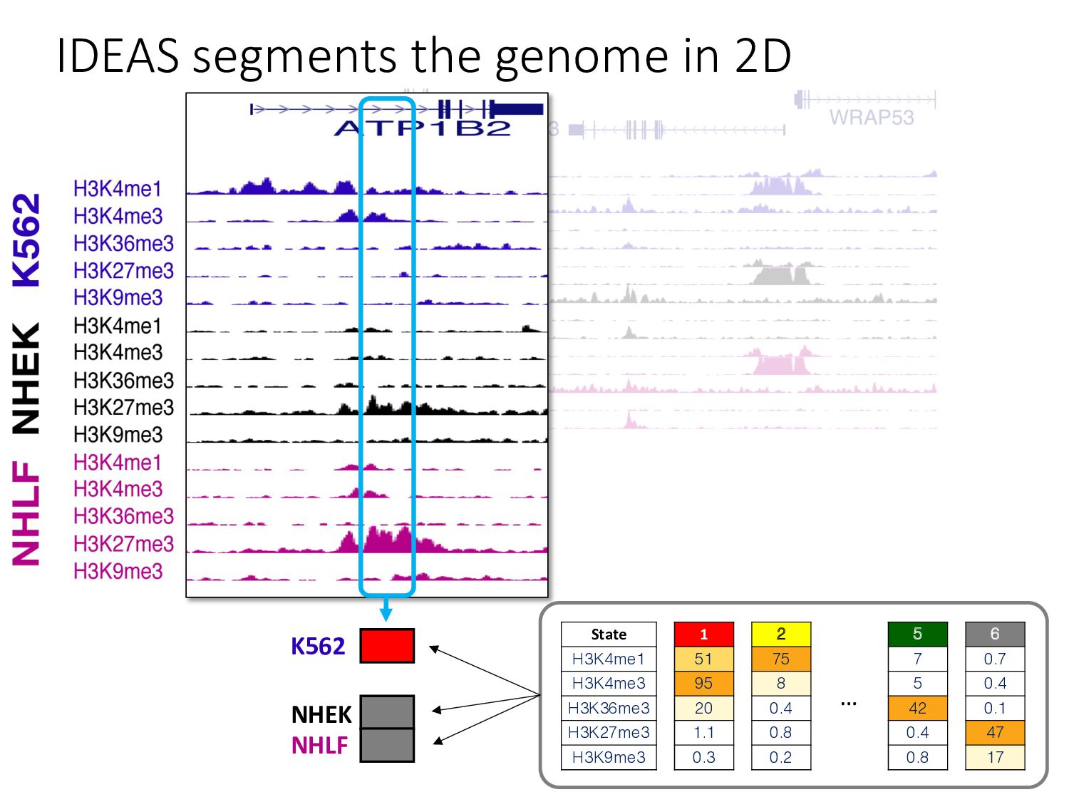
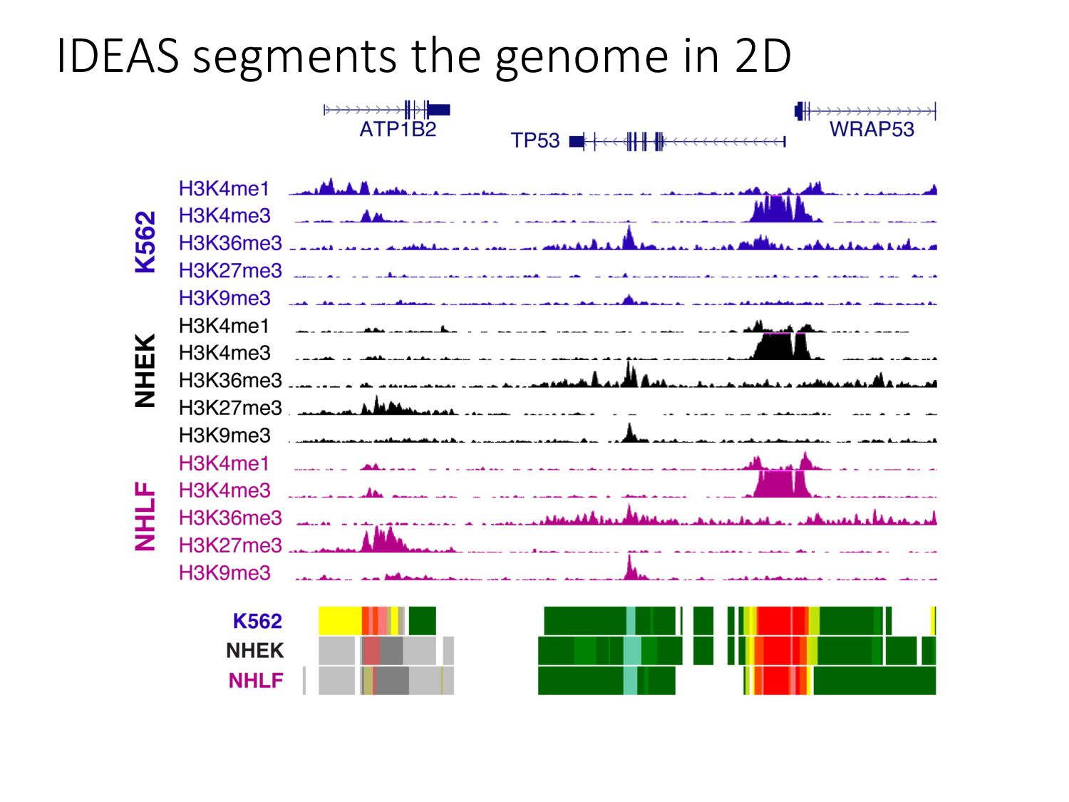
35. “Chromatin state” • A chromatin state is defined by a particular combination of epigenomic activities appearing at the same genomic loci. • Patterns over combinations of: • Histone modifications • Protein-DNA binding • RNA polymerase • DNaseI accessibility • DNA methylation • etc... • Chromatin states correspond to particular modes of functional activity at the underlying regions of the genome.
36. Nucleosome structure • Nucleosome: 147bp wrapped 1.67 times around a histone octamer. • Histone octamer: 2x complexes of H2A-H2B, H3-H4 • Histone tails serve as platforms for epigenetic modifications
37. Histone modifications • Specific positions on histone tails can be chemically modified. • Acetylation (Ac) • Methylation (Me) • Positions can be mono-, di-, or tri-methylated. • Phosphorylation (P) • Ubiquitylation (Ub) • Shorthand notation: • H3K4me3 = Histone 3, Lysine at position 4, tri-methylated • H3K27ac = Histone 3, Lysine at position 27, acetylated • H4R3me2 = Histone 4, Arginine at position 3, di-methylated
38. Histone modifications M = methylation A = acetylation P = phosphorylation U = ubiquitylation
39. Some histone modifications preferentially occur at transcription start sites
40. Histone marks are associated with particular regulatory events • Transcriptional initiation at promoters: • H3K4me3 & H3K9ac • Transcriptional elongation in gene bodies: • H3K79me2 & H3K36me3 • Repressed chromatin: • H3K27me3 or H3K9me3 • Active enhancers: • H3K4me1 and H3K27ac without H3K4me3 • ‘Poised’ enhancers: • H3K4me1 without H3K27ac & H3K4me3
41. The role of histone modifications • Various proteins can recognize/bind to chromatin if particular histone modifications are present. Examples: Trithorax recognizes H3K4me3 Polycomb recognizes H3K27me3
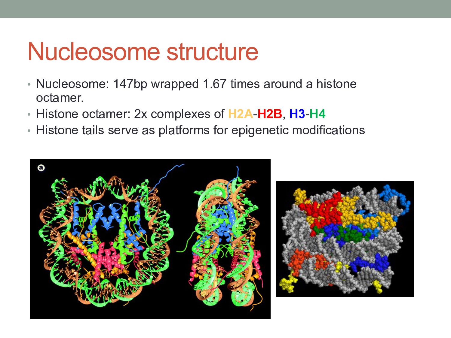
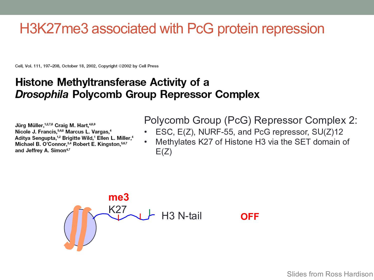
42. H3K27me3 associated with PcG protein repression Polycomb Group (PcG) Repressor Complex 2: • ESC, E(Z), NURF-55, and PcG repressor, SU(Z)12 • Methylates K27 of Histone H3 via the SET domain of E(Z) me3 H3 N-tail K27 OFF Slides from Ross Hardison
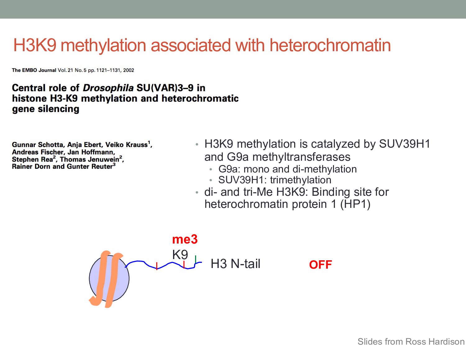
43. H3K9 methylation associated with heterochromatin H3 N-tail me3 K9 OFF • H3K9 methylation is catalyzed by SUV39H1 and G9a methyltransferases • G9a: mono and di-methylation • SUV39H1: trimethylation • di- and tri-Me H3K9: Binding site for heterochromatin protein 1 (HP1) Slides from Ross Hardison
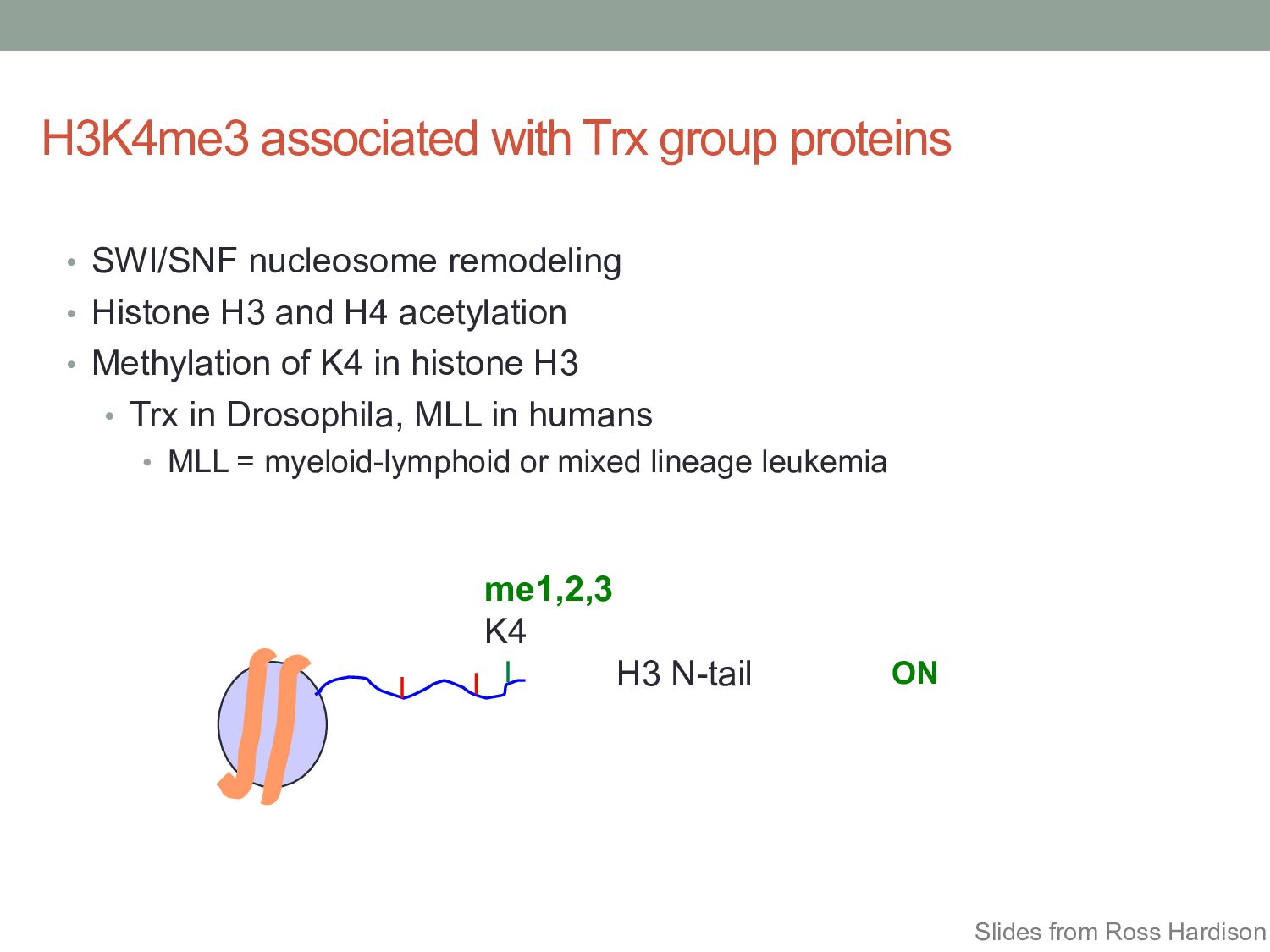
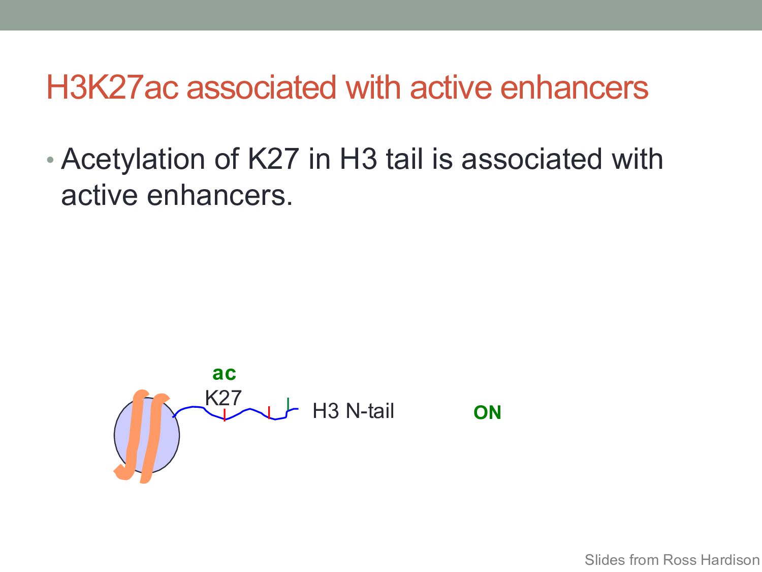
44. H3K4me3 associated with Trx group proteins • SWI/SNF nucleosome remodeling • Histone H3 and H4 acetylation • Methylation of K4 in histone H3 • Trx in Drosophila, MLL in humans • MLL = myeloid-lymphoid or mixed lineage leukemia H3 N-tail me1,2,3 K4 ON Slides from Ross Hardison
45. H3K27ac associated with active enhancers • Acetylation of K27 in H3 tail is associated with active enhancers. ac H3 N-tail K27 ON Slides from Ross Hardison
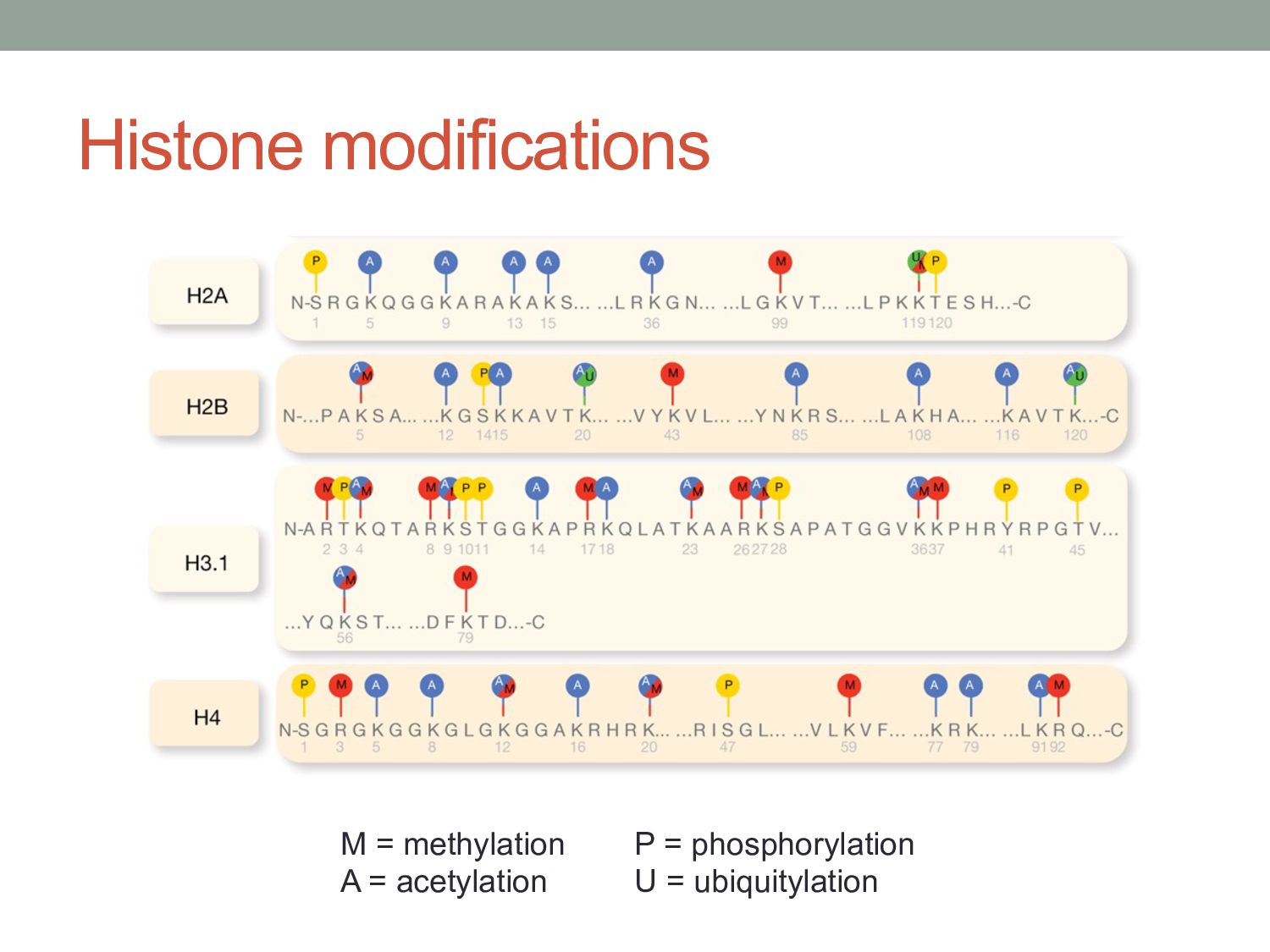
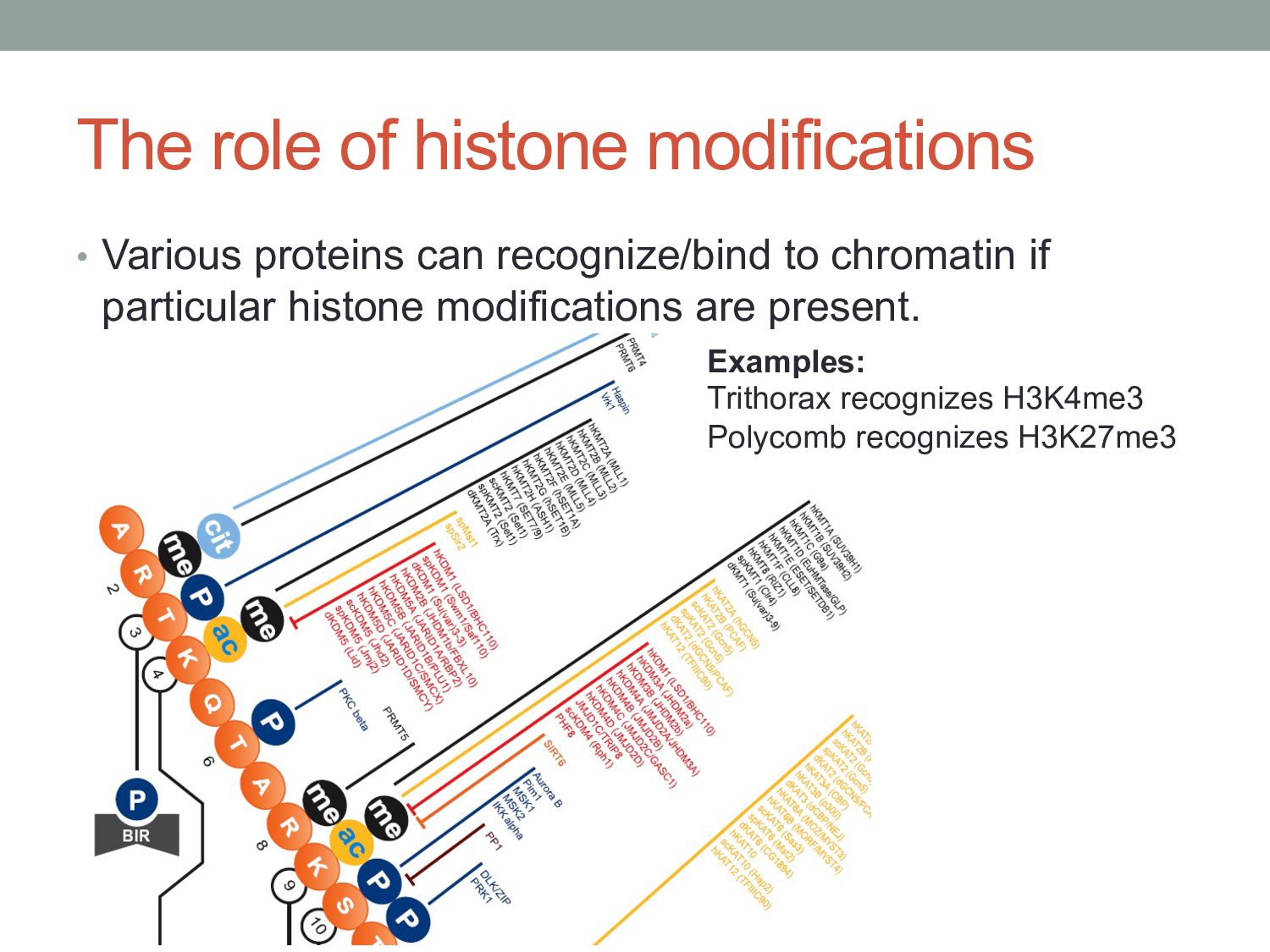
46. The histone code idea • Hypothesis: a “histone code” might exist that extends the information potential of DNA. • Histone modifications and chromatin-associated proteins might serve to store information about the regulatory ‘state’ of underlying genes, and might allow this information to be stably inherited by offspring cells. • Potential complexity of the code is enormous: • e.g. 19 lysine residues on H3 which can be un-, mono-, di-, or tri- methylated… so 419 possible combinations?
47. Assessing the complexity of the histone code. Zhao lab (NIH): • Profiled lots of histone marks in T cells. • Correlated presence of marks over the genome.
48. ENCODE: an encyclopedia of functional elements ENCODE consortium, 2011, PLoS Biology 9: e1001046
49. Distinctive patterns of histone marks across transcribed genes K4me3àK79me2 àK36me3 Bernstein lab, ENCODE H3K4me3 H3K79me2 H3K36me3
50. Genome segmentation enables annotation of regulatory activities K562 State H3K4me1 H3K4me3 H3K36me3 H3K27me3 H3K9me3 1 51 95 20 1.1 0.3 2 75 8 0.4 0.8 0.2 5 7 5 42 0.4 0.8 6 0.7 0.4 0.1 47 17 … TSS Enhancer Elongation Repressed
51. Segmentation should be consistent across cell types Assumptions: • State identities shared across cell types • Locus may display same regulatory state in multiple cell types.
52. 1D strategies for multi-cell segmentation discard positional information … … Treat data as if it arises from N concatenated genomes … ignore position specificity
53. 1D strategies for multi-cell segmentation discard positional information … … State H3K4me1 H3K4me3 H3K36me3 H3K27me3 H3K9me3 1 51 95 20 1.1 0.3 2 75 8 0.4 0.8 0.2 5 7 5 42 0.4 0.8 6 0.7 0.4 0.1 47 17 … TSS Enhancer Elongation Repressed … …
54. IDEAS segments the genome in 2D IDEAS: Integrative and Discriminative Epigenomic Annotation System Zhang et al. NAR 2016; Zhang and Hardison, NAR 2017
55. IDEAS segments the genome in 2D State H3K4me1 H3K4me3 H3K36me3 H3K27me3 H3K9me3 1 51 95 20 1.1 0.3 2 75 8 0.4 0.8 0.2 5 7 5 42 0.4 0.8 6 0.7 0.4 0.1 47 17 …
56. IDEAS segments the genome in 2D State H3K4me1 H3K4me3 H3K36me3 H3K27me3 H3K9me3 1 51 95 20 1.1 0.3 2 75 8 0.4 0.8 0.2 5 7 5 42 0.4 0.8 6 0.7 0.4 0.1 47 17 … K562 NHEK NHLF ? ? ?
57. IDEAS segments the genome in 2D State H3K4me1 H3K4me3 H3K36me3 H3K27me3 H3K9me3 1 51 95 20 1.1 0.3 2 75 8 0.4 0.8 0.2 5 7 5 42 0.4 0.8 6 0.7 0.4 0.1 47 17 …
58. IDEAS segments the genome in 2D State H3K4me1 H3K4me3 H3K36me3 H3K27me3 H3K9me3 1 51 95 20 1.1 0.3 2 75 8 0.4 0.8 0.2 5 7 5 42 0.4 0.8 6 0.7 0.4 0.1 47 17 … K562 NHEK NHLF
59. IDEAS segments the genome in 2D
60. Challenges in chromatin state analysis • How many states are there? • How do chromatin states change across cell types? • What do chromatin states tell us about human genetics & health? • Study variants in functional regions as annotated by HMMs using GWAS. • Examine how chromatin state changes between normal & disease tissues.
61. Further reading • Discovery and characterization of chromatin states for systematic annotation of the human genome. Ernst & Kellis Nature Biotechnology (2010)