Lecture 18 RNA-seq II

BMMB 554 Lecture 18

Transcript

1. L18: RNA-SEQ II Foundations in Data Driven Life Sciences BMMB/MCIBS 554
2. Today’s learning objectives • Understand statistical approaches to modeling count data from functional genomics experiments. • Discuss other challenges in RNA-seq analysis. • Learn about RNA-seq quantification approaches.
3. The Negative Binomial Distribution • Used when the rate of a Poisson process is itself varying
4. Sample-to-sample variation average per-gene count Comparison of two biological replicates Comparison of treatment vs control average per-gene count
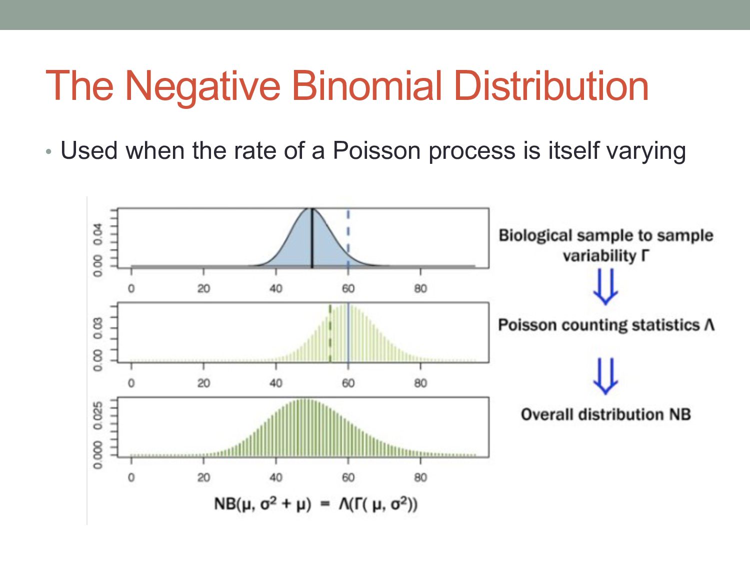
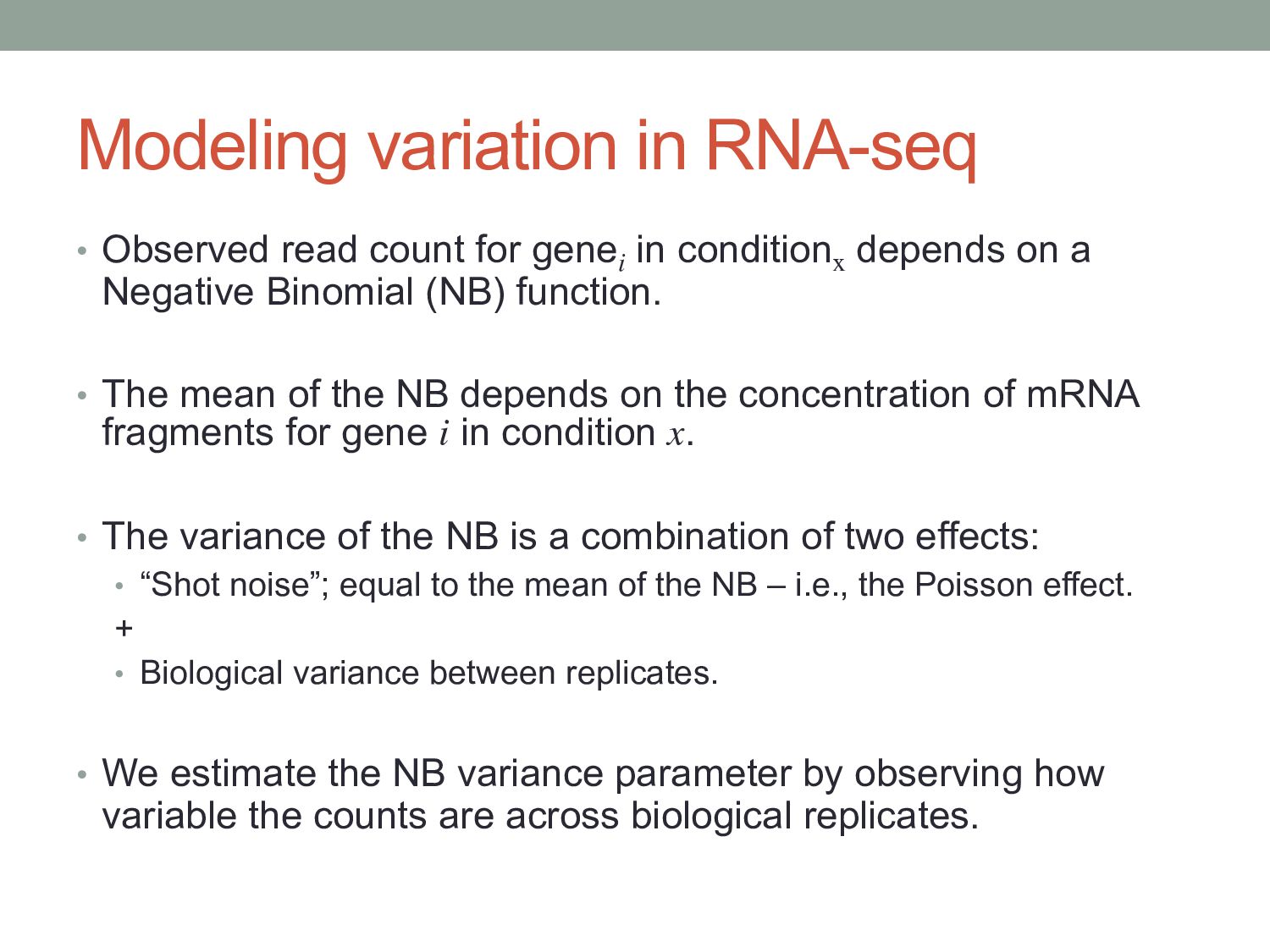
5. Modeling variation in RNA-seq • Observed read count for gene i in conditionx depends on a Negative Binomial (NB) function. • The mean of the NB depends on the concentration of mRNA fragments for gene i in condition x. • The variance of the NB is a combination of two effects: • “Shot noise”; equal to the mean of the NB – i.e., the Poisson effect. + • Biological variance between replicates. • We estimate the NB variance parameter by observing how variable the counts are across biological replicates.
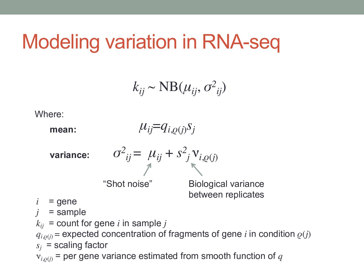
6. Modeling variation in RNA-seq kij ~ NB(μij , σ2 ij ) i = gene j = sample kij = count for gene i in sample j qi,ρ(j) = expected concentration of fragments of gene i in condition ρ(j) sj = scaling factor νi,ρ(j) = per gene variance estimated from smooth function of q Where: μij =qi,ρ(j) sj σ2 ij = μij + s2 j νi,ρ(j) “Shot noise” Biological variance between replicates mean: variance:
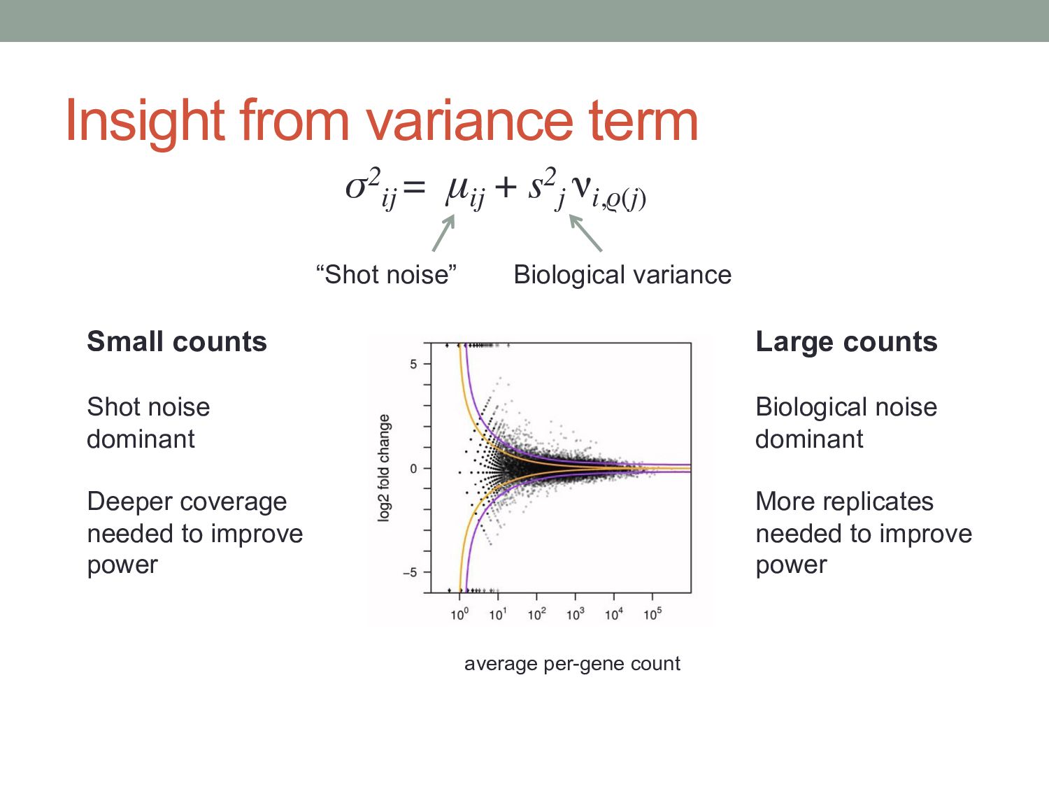
7. Insight from variance term average per-gene count σ2 ij = μij + s2 j νi,ρ(j) “Shot noise” Biological variance Small counts Shot noise dominant Deeper coverage needed to improve power Large counts Biological noise dominant More replicates needed to improve power
8. Sharing estimates of dispersion across genes
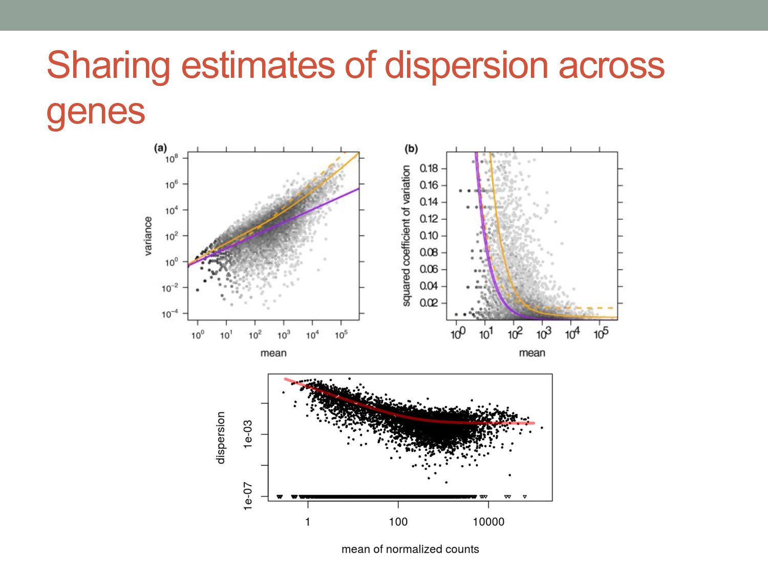
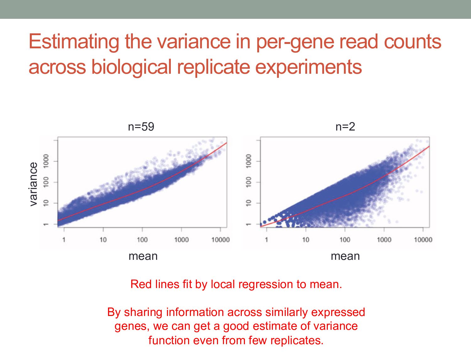
9. Estimating the variance in per-gene read counts across biological replicate experiments n=59 n=2 mean mean variance Red lines fit by local regression to mean. By sharing information across similarly expressed genes, we can get a good estimate of variance function even from few replicates.
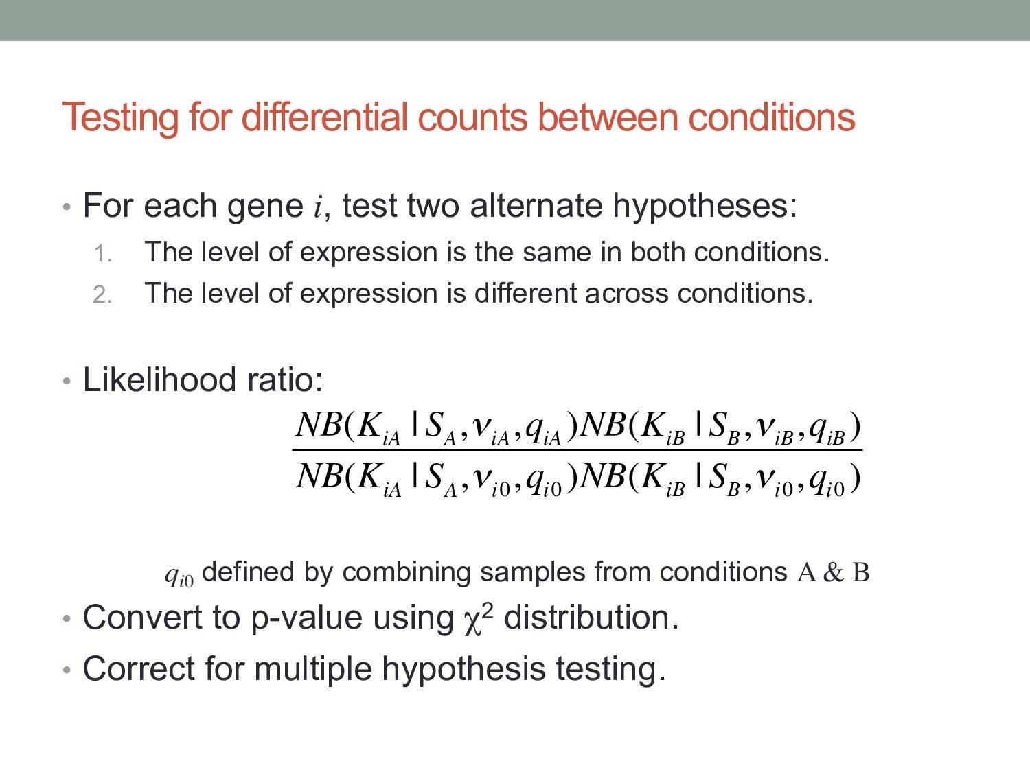
10. Testing for differential counts between conditions • For each gene i, test two alternate hypotheses: 1. The level of expression is the same in both conditions. 2. The level of expression is different across conditions. • Likelihood ratio: qi0 defined by combining samples from conditions A & B • Convert to p-value using χ2 distribution. • Correct for multiple hypothesis testing. NB(K iA | S A ,νiA ,q iA )NB(K iB | S B ,νiB ,q iB ) NB(K iA | S A ,νi0 ,q i0 )NB(K iB | S B ,νi0 ,q i0 )
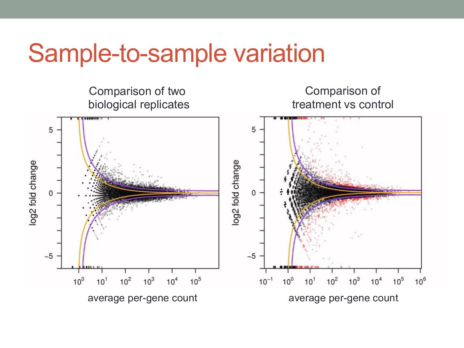
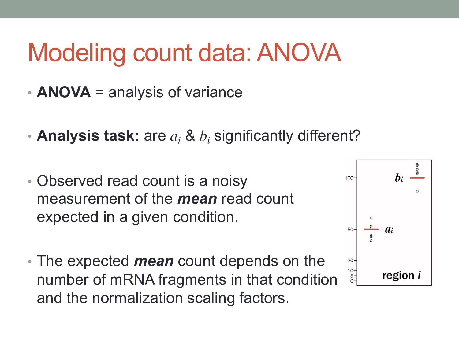
11. Modeling count data: ANOVA • ANOVA = analysis of variance • Analysis task: are ai & bi significantly different? • Observed read count is a noisy measurement of the mean read count expected in a given condition. • The expected mean count depends on the number of mRNA fragments in that condition and the normalization scaling factors.
12. Significance cut-off for determining differential counts average per-gene count Comparison of two biological replicates Comparison of two treatment vs control average per-gene count
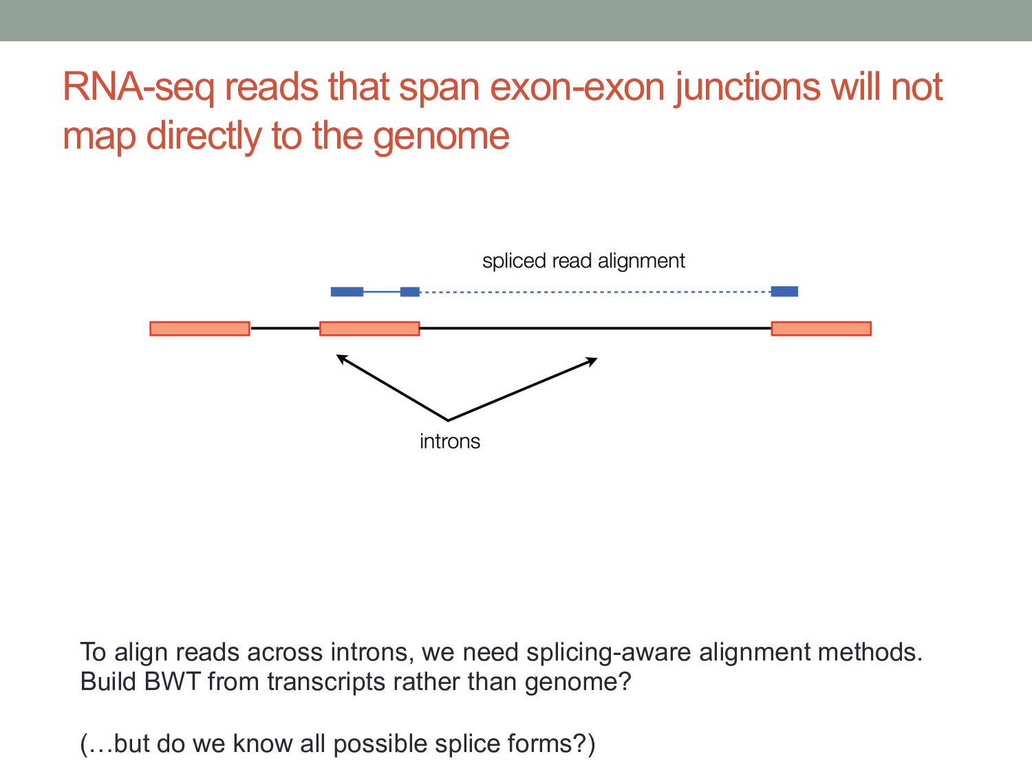
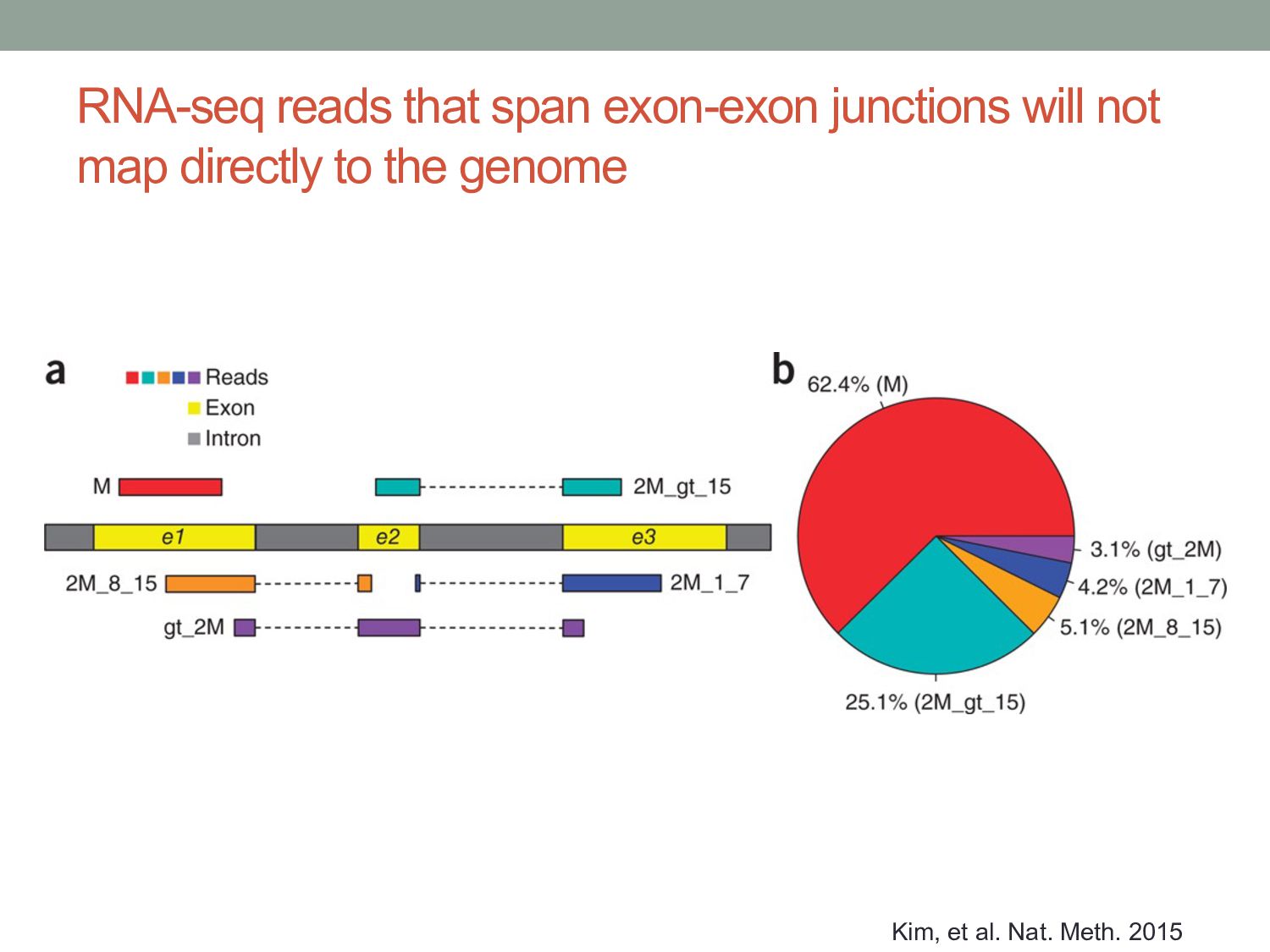
13. RNA-seq reads that span exon-exon junctions will not map directly to the genome To align reads across introns, we need splicing-aware alignment methods. Build BWT from transcripts rather than genome? (…but do we know all possible splice forms?)
14. RNA-seq reads that span exon-exon junctions will not map directly to the genome Kim, et al. Nat. Meth. 2015
15. How do we map to unknown exon-exon boundaries?
16. TopHat
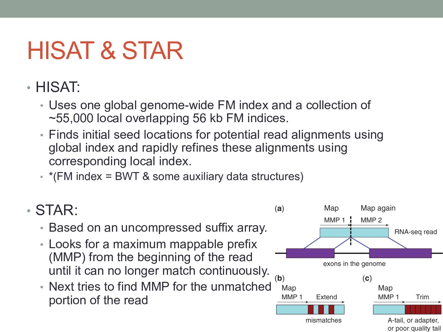
17. HISAT & STAR • HISAT: • Uses one global genome-wide FM index and a collection of ~55,000 local overlapping 56 kb FM indices. • Finds initial seed locations for potential read alignments using global index and rapidly refines these alignments using corresponding local index. • *(FM index = BWT & some auxiliary data structures) • STAR: • Based on an uncompressed suffix array. • Looks for a maximum mappable prefix (MMP) from the beginning of the read until it can no longer match continuously. • Next tries to find MMP for the unmatched portion of the read
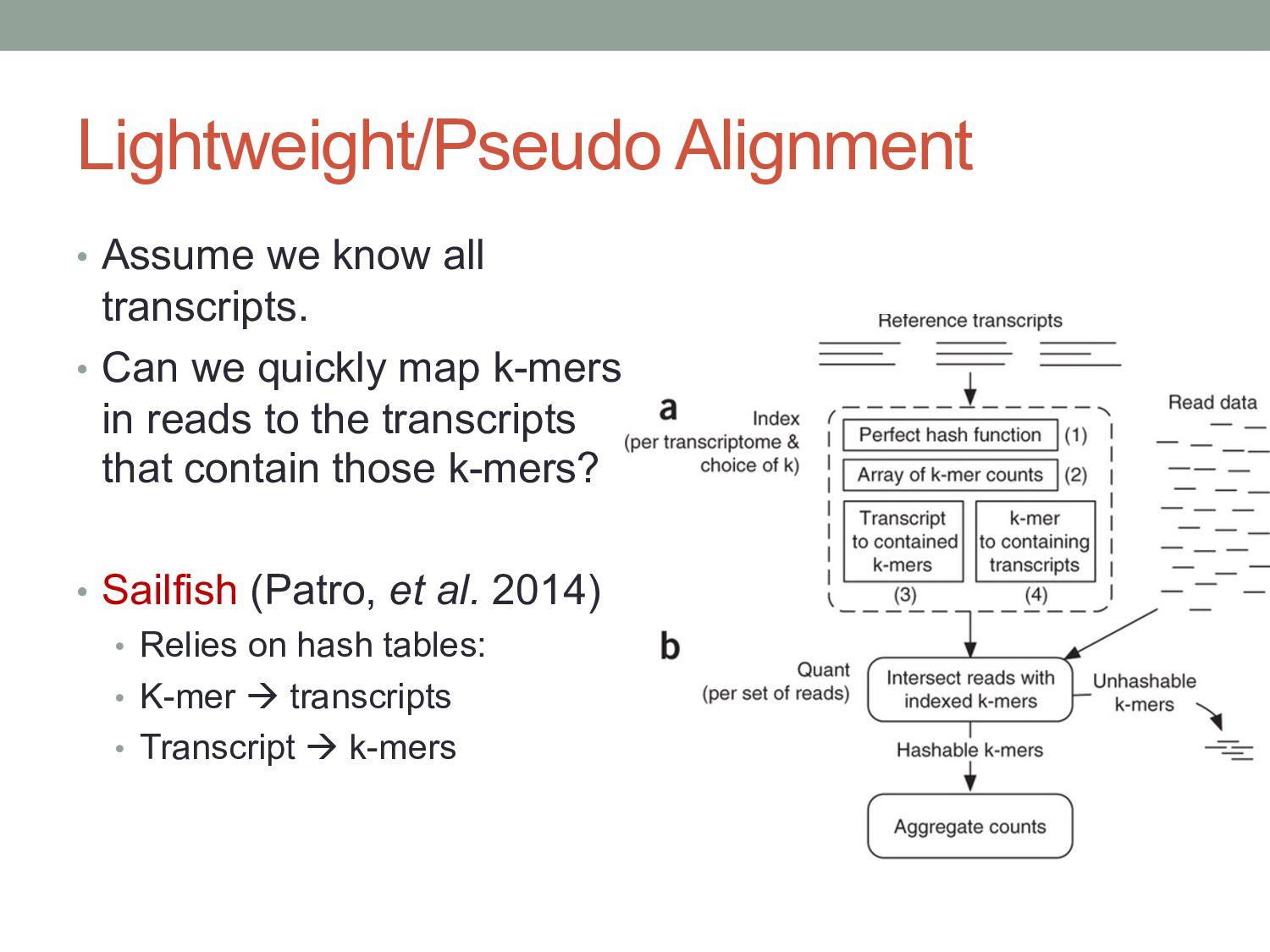
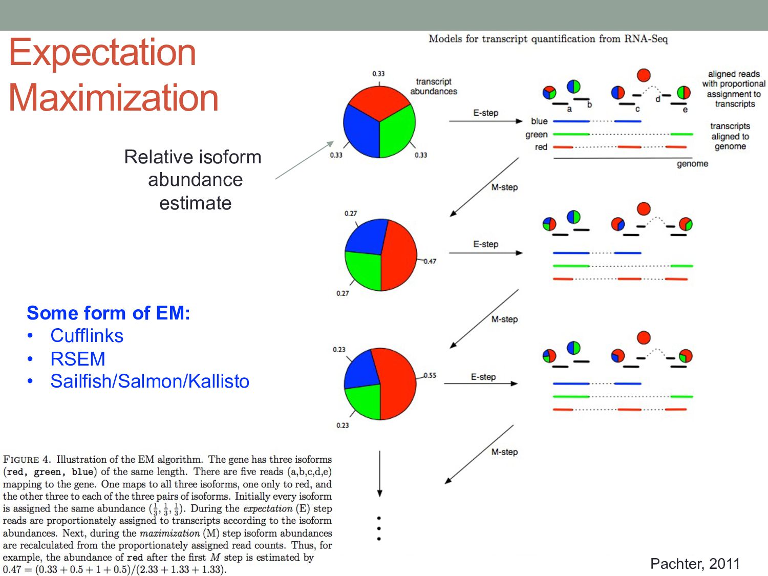
18. Lightweight/Pseudo Alignment • Assume we know all transcripts. • Can we quickly map k-mers in reads to the transcripts that contain those k-mers? • Sailfish (Patro, et al. 2014) • Relies on hash tables: • K-mer à transcripts • Transcript à k-mers
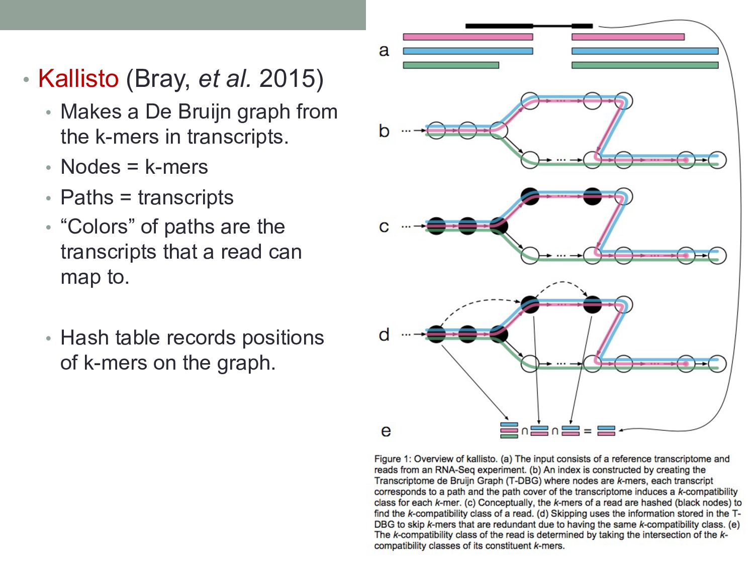
19. • Kallisto (Bray, et al. 2015) • Makes a De Bruijn graph from the k-mers in transcripts. • Nodes = k-mers • Paths = transcripts • “Colors” of paths are the transcripts that a read can map to. • Hash table records positions of k-mers on the graph.
20. • Salmon (Patro, et al. 2015) • Quasi-alignment • Relies on a suffix array and a hash table (k-mer à position on suffix array). • Looks for chains of Maximal Exact Matches (MEMs).
21. Can RNA-seq tell us which isoforms are expressed? Reads Transcripts • Genes can have many isoforms, making it challenging to determine which isoform produced each read.
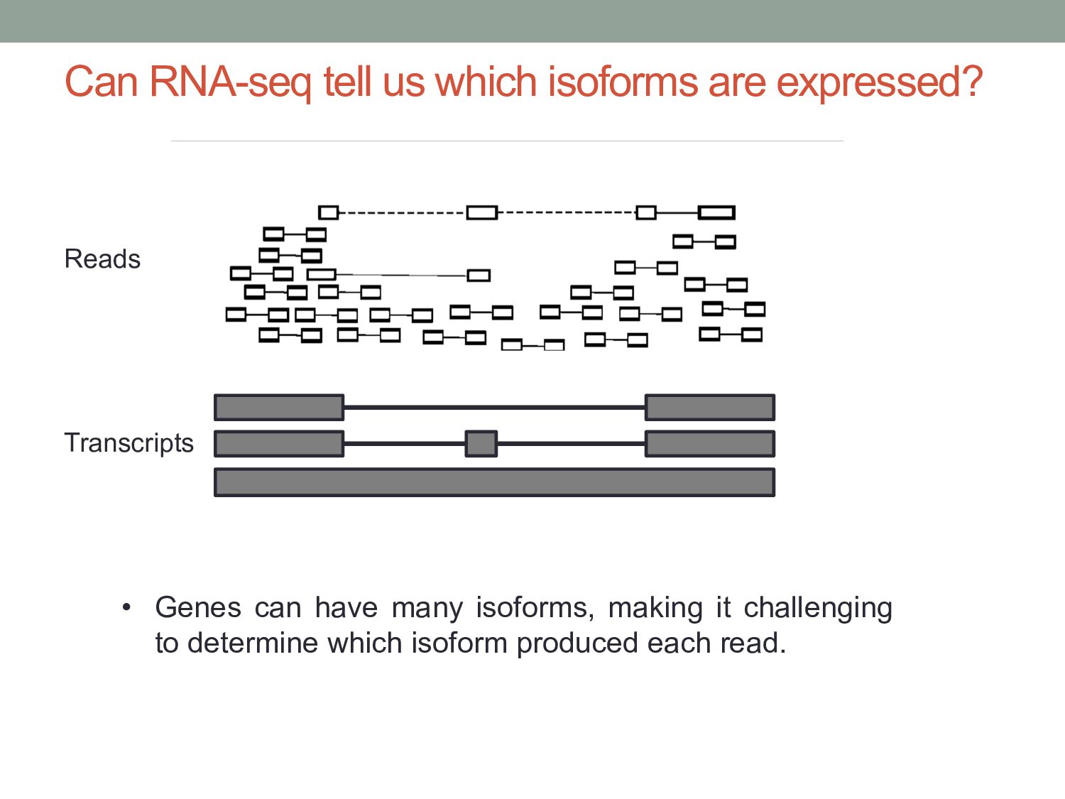
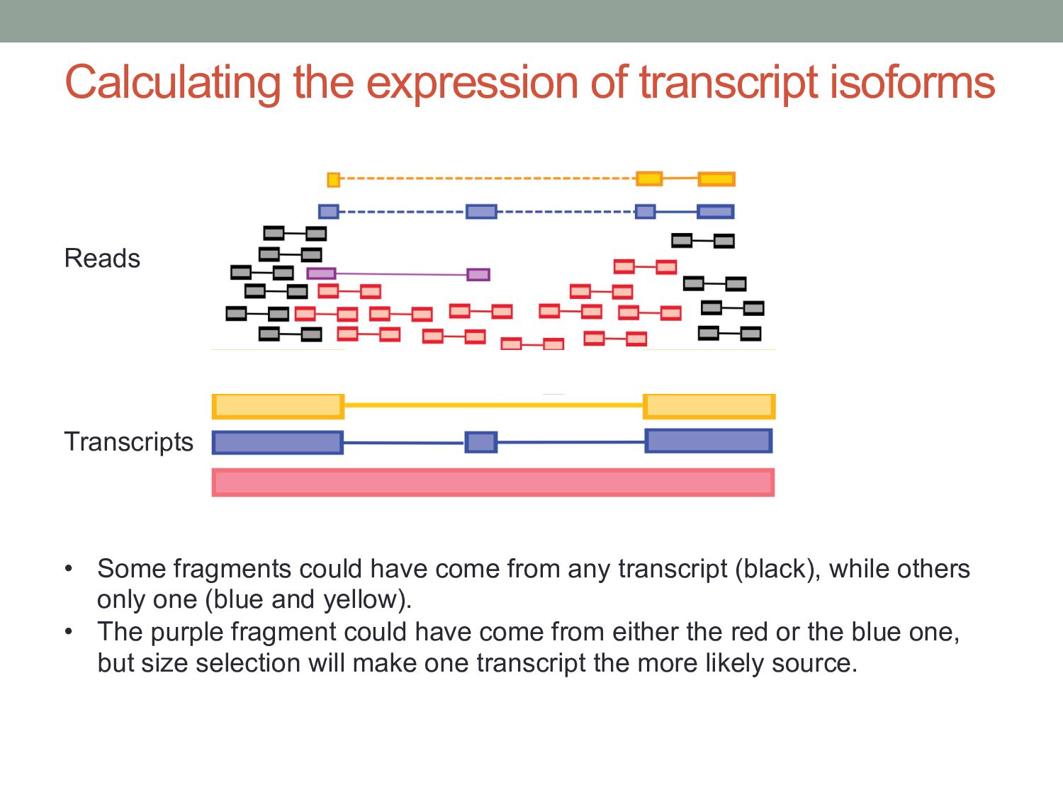
22. Calculating the expression of transcript isoforms • Some fragments could have come from any transcript (black), while others only one (blue and yellow). • The purple fragment could have come from either the red or the blue one, but size selection will make one transcript the more likely source. Reads Transcripts
23. Expectation Maximization Pachter, 2011 Relative isoform abundance estimate
24. Expectation Maximization Pachter, 2011 Relative isoform abundance estimate
25. Expectation Maximization Pachter, 2011 Relative isoform abundance estimate Some form of EM: • Cufflinks • RSEM • Sailfish/Salmon/Kallisto
26. Transcript assembly without a reference
27. StringTie Pertea, et al. Nat. Biotech. 2015
28. RNA-seq tutorial • https://training.galaxyproject.org/training- material/topics/transcriptomics/tutorials/rb- rnaseq/tutorial.html
29. Summary • We’re often interested in discovering how biochemical activities vary across cell types or conditions. With functional genomics assays, this involves analyzing differences in read count information. • Statistical analysis of sequencing (count-based) data needs to account for many sources of variance. • Differentially expressed genes can be found using statistical tests based on the Negative Binomial distribution. • Aligning/quantifying reads to the transcriptome requires methods that are splicing-aware. • Different (pseudo-)alignment methods have trade-offs in speed and sensitivity.