Lecture 17: RNA-seq I

BMMB 554 Lecture 17

Transcript

1. L17: RNA-SEQ I Foundations in Data Driven Life Sciences BMMB/MCIBS 554
2. Today’s learning objectives • Learn how RNA-seq enables transcript abundance measurements. • Understand statistical approaches to modeling count data from functional genomics experiments. • Discuss other challenges in RNA-seq analysis Some material adapted from: Cole Trapnell Wolfgang Huber
3. RNA-seq
4. RNA-seq experimental considerations 1) Isolate RNA: RNA extraction, DNase treatment 2) RNA selection: • Total RNA • PolyA-selection: hybridize to poly(T) oligos attached to beads • rRNA depletion: hybridize to rRNA-specific oligos • Size selection
5. RNA-seq experimental considerations 3) cDNA synthesis Random priming Oligo-dT priming How do we retain strandedness?
6. RNA-seq Illumina TruSeq dUTPs incorporated
7. The more abundant a transcript is, the more fragments we’ll sequence from it Slide adapted from Cole Trapnell RNA-seq
8. RNA-seq Slide adapted from Cole Trapnell
9. Some sources of noise in RNA-seq count data • Gene length • PCR bias • “Sequenceability” • 3’ bias Varies locally along gene
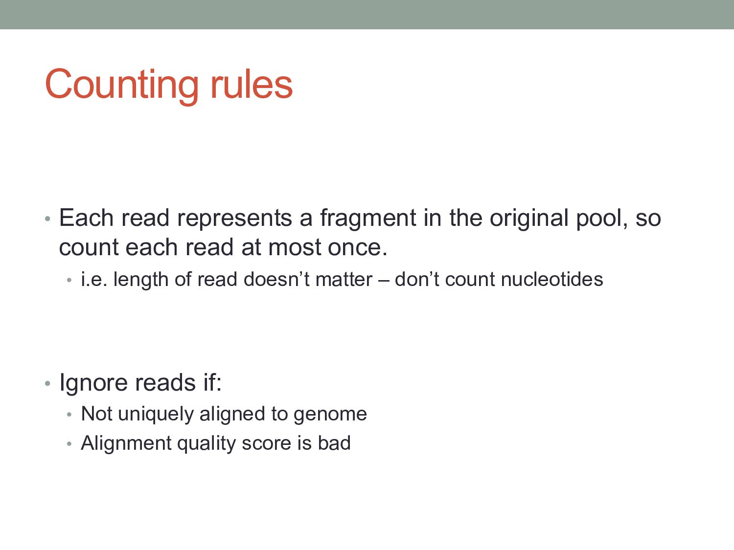
10. Counting rules • Each read represents a fragment in the original pool, so count each read at most once. • i.e. length of read doesn’t matter – don’t count nucleotides • Ignore reads if: • Not uniquely aligned to genome • Alignment quality score is bad
11. RNA-seq (and *-seq) produces count data Gene C1_r1 C1_r2 C2_r1 C2_r2 C3_r1 C3_r2 C4_r1 C4r2 ENSMUSG00000061501 0 0 0 0 0 0 0 0 ENSMUSG00000039377 1 0 0 0 3 0 0 0 ENSMUSG00000039376 5 13 10 10 40 3 16 0 ENSMUSG00000039375 205 193 149 94 203 142 273 108 ENSMUSG00000012848 22011 3367 16112 2971 14393 2781 15096 2482 ENSMUSG00000003269 1547 1710 1411 1751 2327 2094 1497 1655 ENSMUSG00000039385 3185 1628 2470 2161 4490 3118 3209 3078 ENSMUSG00000039382 307 463 236 206 419 295 241 257 ENSMUSG00000039384 734 298 630 283 973 324 469 179 ENSMUSG00000010592 0 0 2 0 0 0 0 0 ENSMUSG00000040701 353 369 282 516 746 505 239 385 Tens of thousands of rows
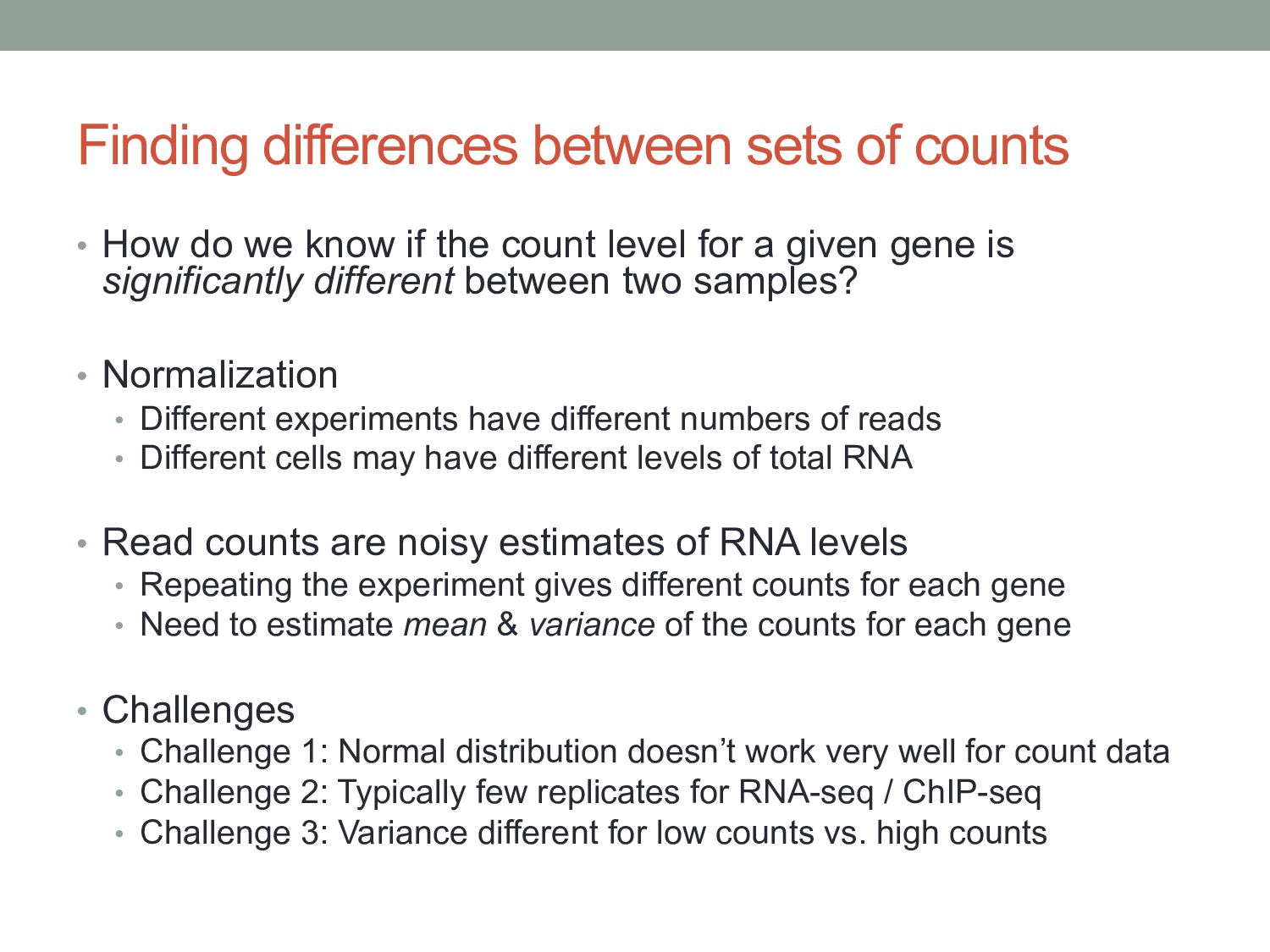
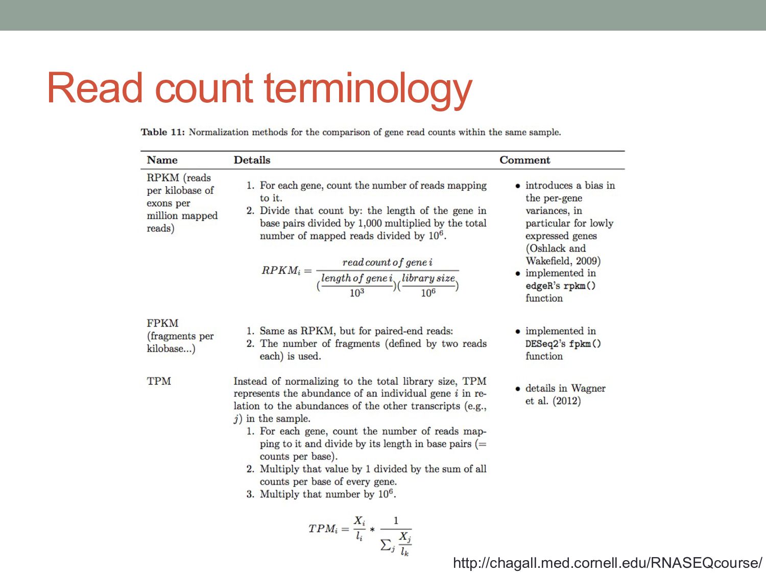
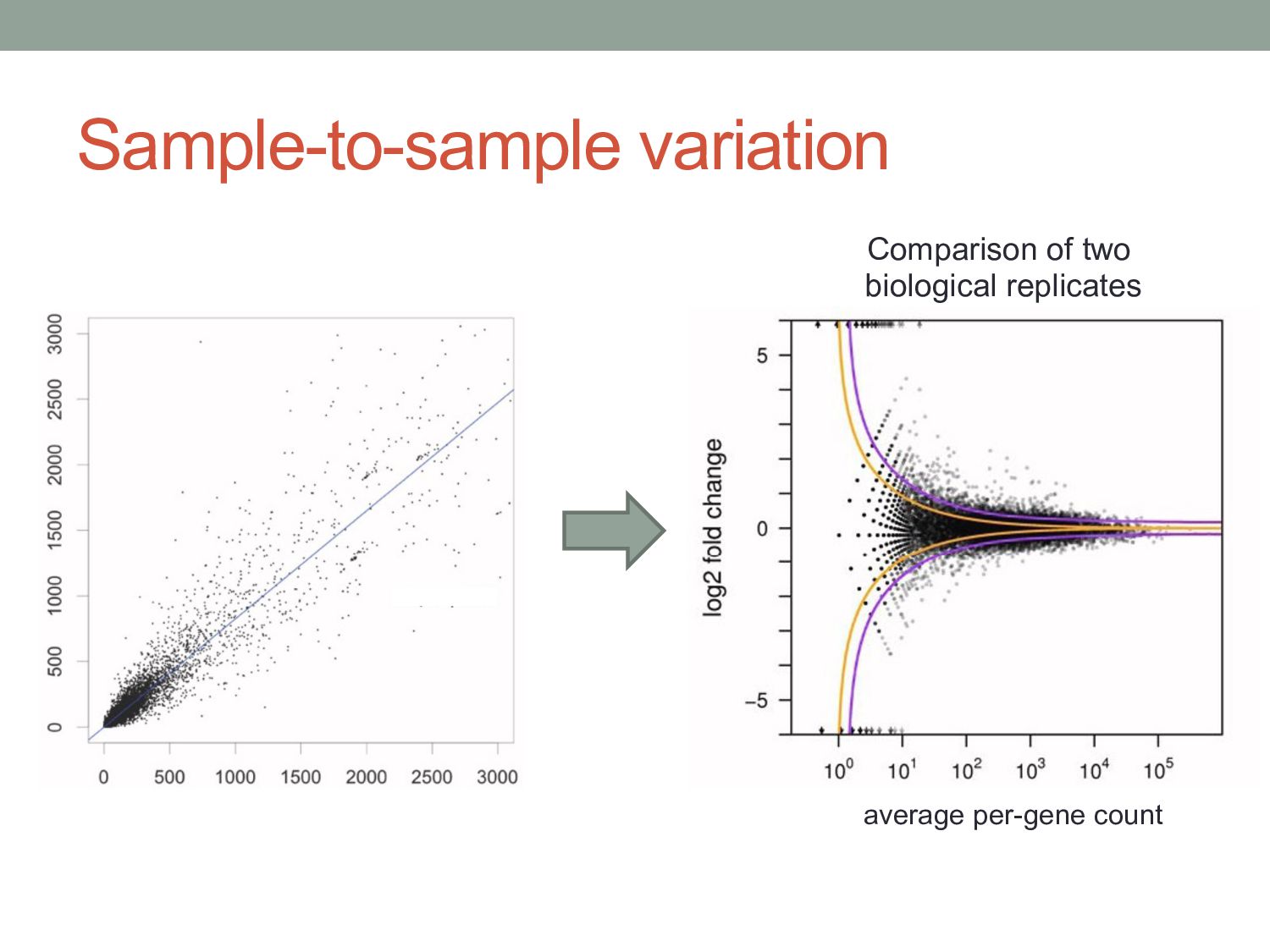
12. Finding differences between sets of counts • How do we know if the count level for a given gene is significantly different between two samples? • Normalization • Different experiments have different numbers of reads • Different cells may have different levels of total RNA • Read counts are noisy estimates of RNA levels • Repeating the experiment gives different counts for each gene • Need to estimate mean & variance of the counts for each gene • Challenges • Challenge 1: Normal distribution doesn’t work very well for count data • Challenge 2: Typically few replicates for RNA-seq / ChIP-seq • Challenge 3: Variance different for low counts vs. high counts
13. Read count terminology http://chagall.med.cornell.edu/RNASEQcourse/
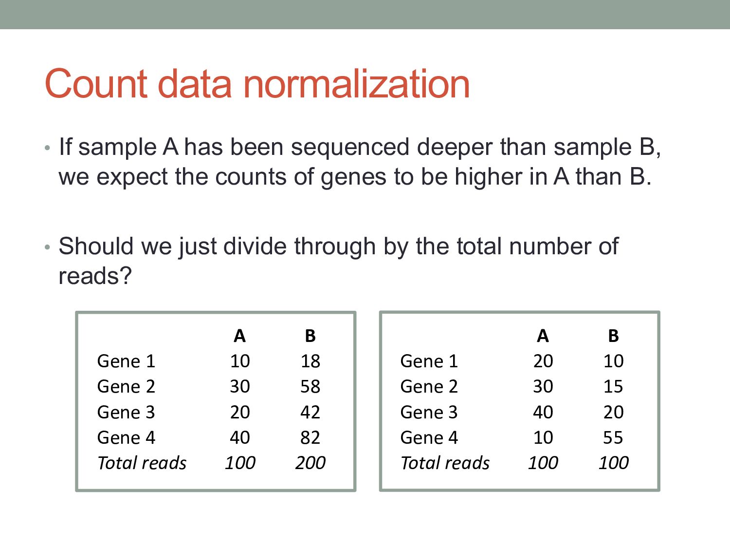
14. Count data normalization • If sample A has been sequenced deeper than sample B, we expect the counts of genes to be higher in A than B. • Should we just divide through by the total number of reads? A B Gene 1 10 18 Gene 2 30 58 Gene 3 20 42 Gene 4 40 82 Total reads 100 200 A B Gene 1 20 10 Gene 2 30 15 Gene 3 40 20 Gene 4 10 55 Total reads 100 100
15. Normalizing one experiment against another Experiment 1 Experiment 2 Possible approaches: • Fit a regression line • Find median ratio between counts
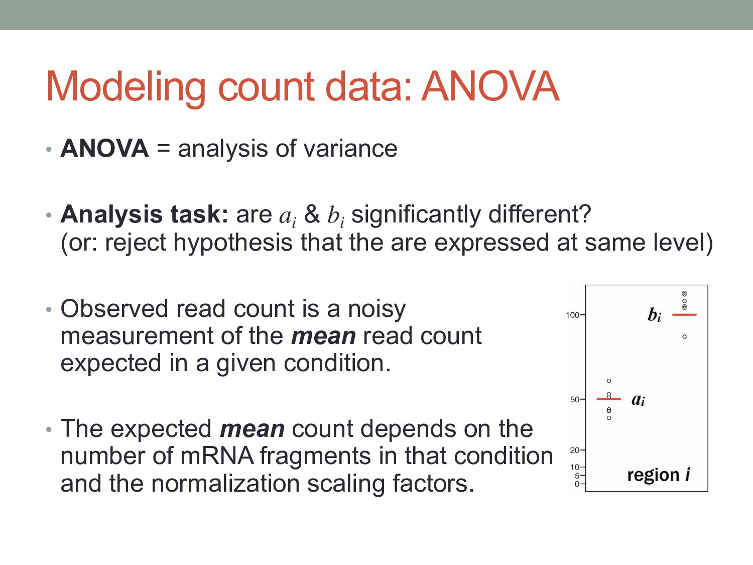
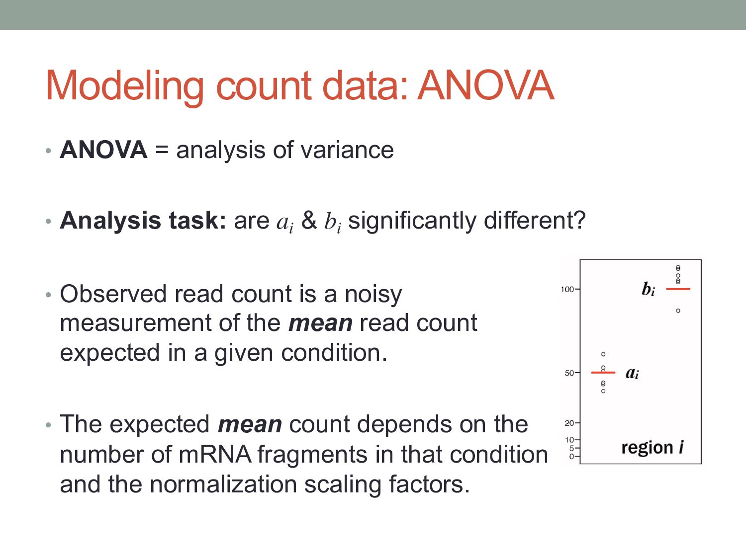
16. Modeling count data: ANOVA • ANOVA = analysis of variance • Analysis task: are ai & bi significantly different? (or: reject hypothesis that the are expressed at same level) • Observed read count is a noisy measurement of the mean read count expected in a given condition. • The expected mean count depends on the number of mRNA fragments in that condition and the normalization scaling factors.
17. Sample-to-sample variation average per-gene count Comparison of two biological replicates
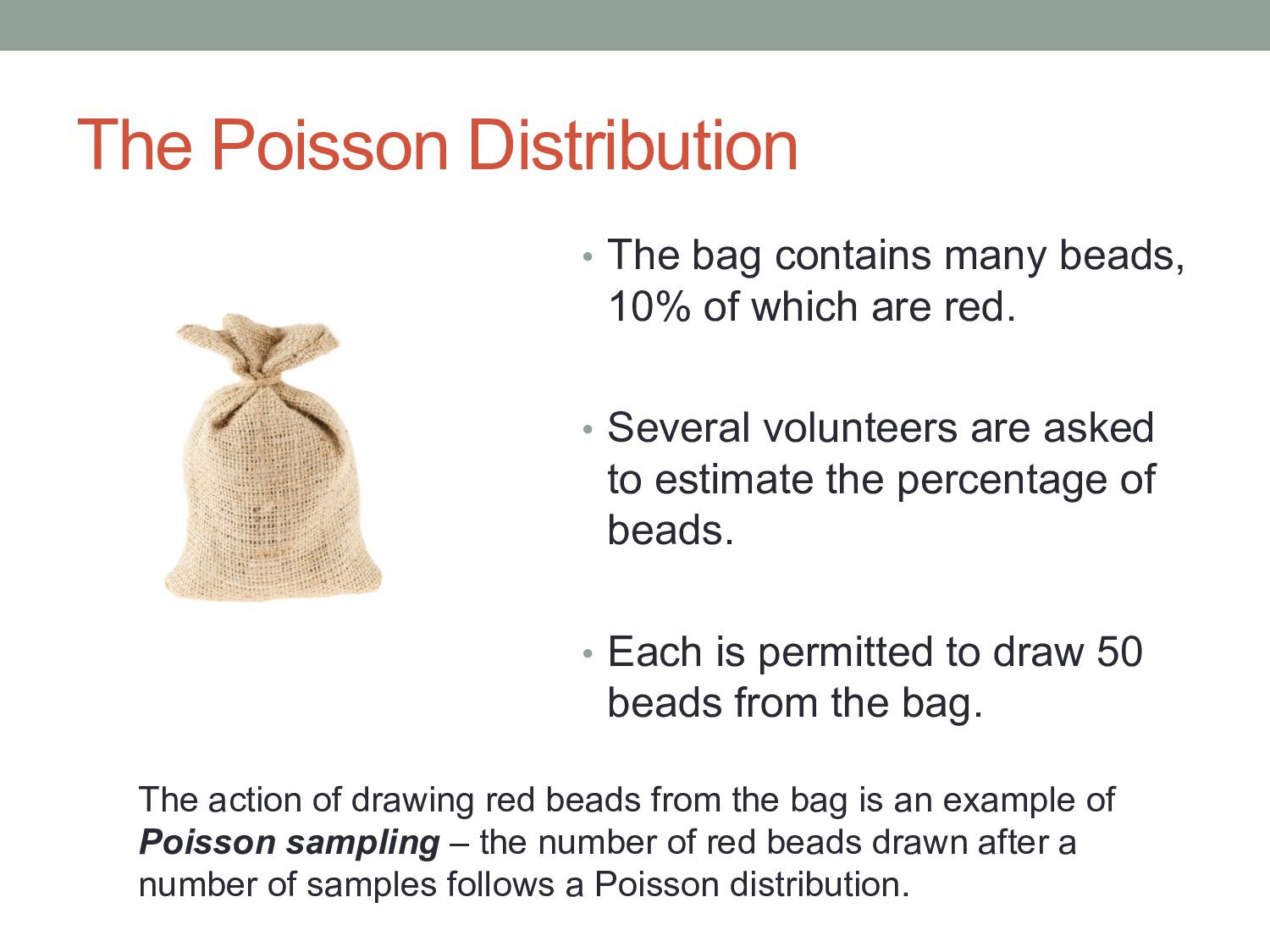
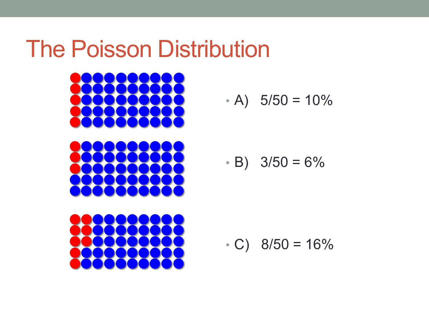
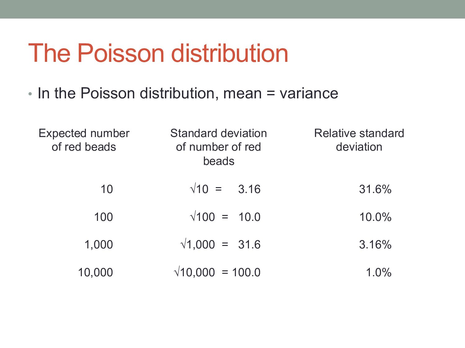
18. The Poisson Distribution • The bag contains many beads, 10% of which are red. • Several volunteers are asked to estimate the percentage of beads. • Each is permitted to draw 50 beads from the bag. The action of drawing red beads from the bag is an example of Poisson sampling – the number of red beads drawn after a number of samples follows a Poisson distribution.
19. The Poisson Distribution • A) 5/50 = 10% • B) 3/50 = 6% • C) 8/50 = 16%
20. The Poisson Distribution • 97/1000 = 9.7% • 107/1000 = 10.7% • 105/1000 = 10.5%
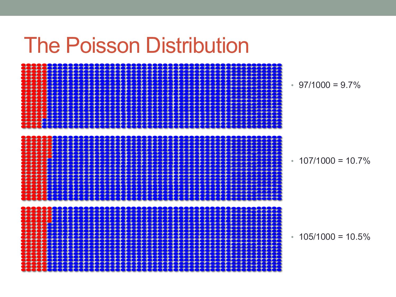
21. The Poisson distribution • In the Poisson distribution, mean = variance Expected number of red beads Standard deviation of number of red beads Relative standard deviation 10 100 1,000 10,000 √10 = 3.16 √100 = 10.0 √1,000 = 31.6 √10,000 = 100.0 31.6% 10.0% 3.16% 1.0%
22. Is the Poisson distribution suitable for modeling RNA-seq variation? Technical replicates Biological replicates σ µ ! " # $ % & 2 Consistent with Poisson Larger than Poisson
23. The Negative Binomial Distribution • Used when the rate of a Poisson process is itself varying
24. Sample-to-sample variation average per-gene count Comparison of two biological replicates Comparison of treatment vs control average per-gene count
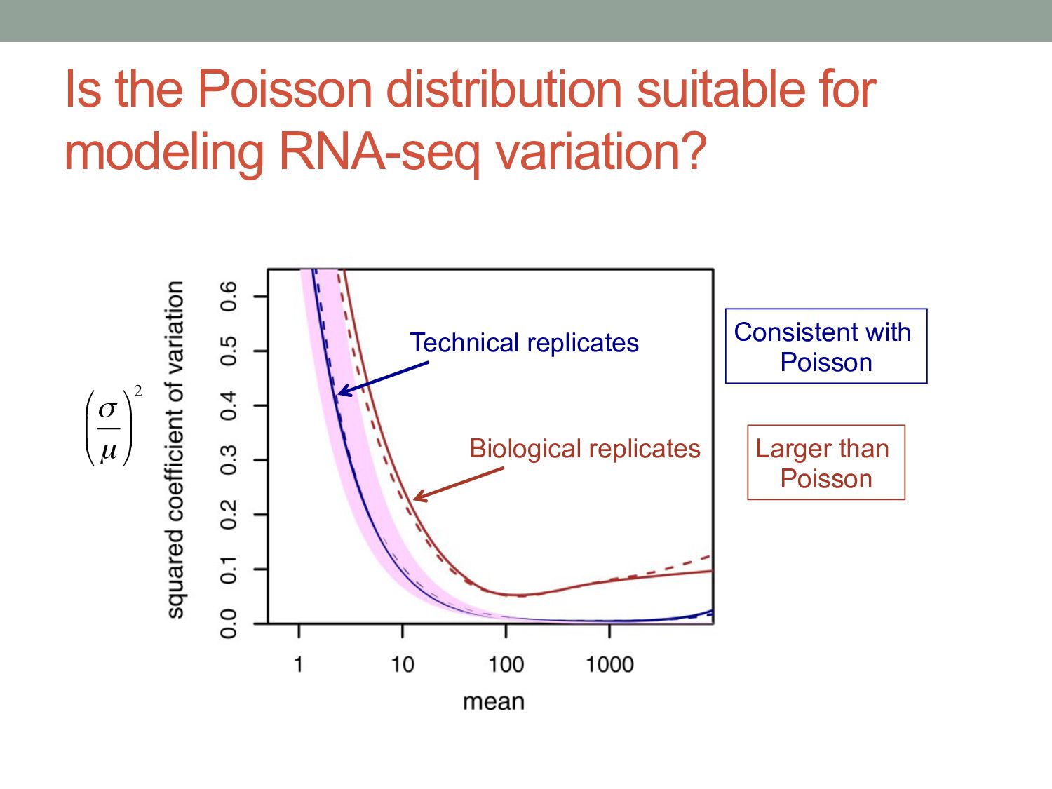
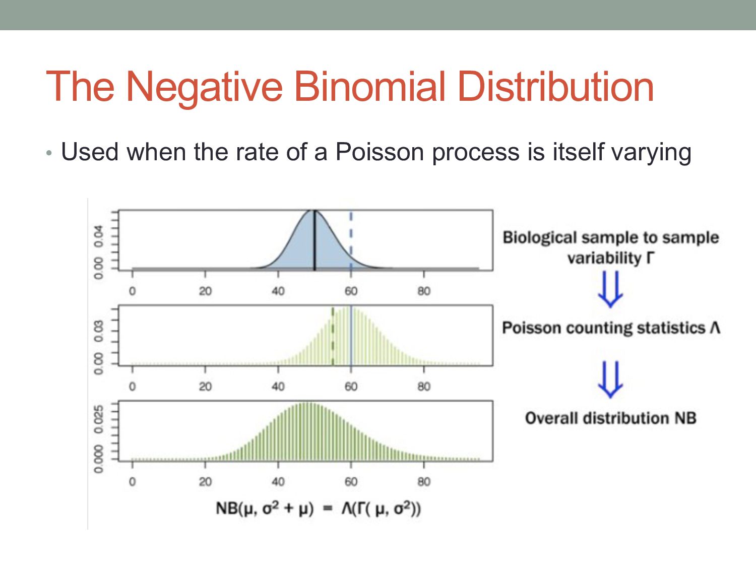
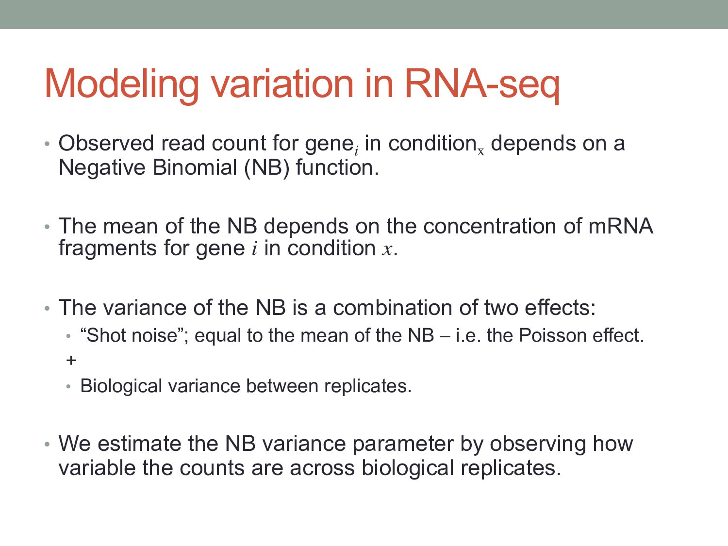
25. Modeling variation in RNA-seq • Observed read count for gene i in conditionx depends on a Negative Binomial (NB) function. • The mean of the NB depends on the concentration of mRNA fragments for gene i in condition x. • The variance of the NB is a combination of two effects: • “Shot noise”; equal to the mean of the NB – i.e. the Poisson effect. + • Biological variance between replicates. • We estimate the NB variance parameter by observing how variable the counts are across biological replicates.
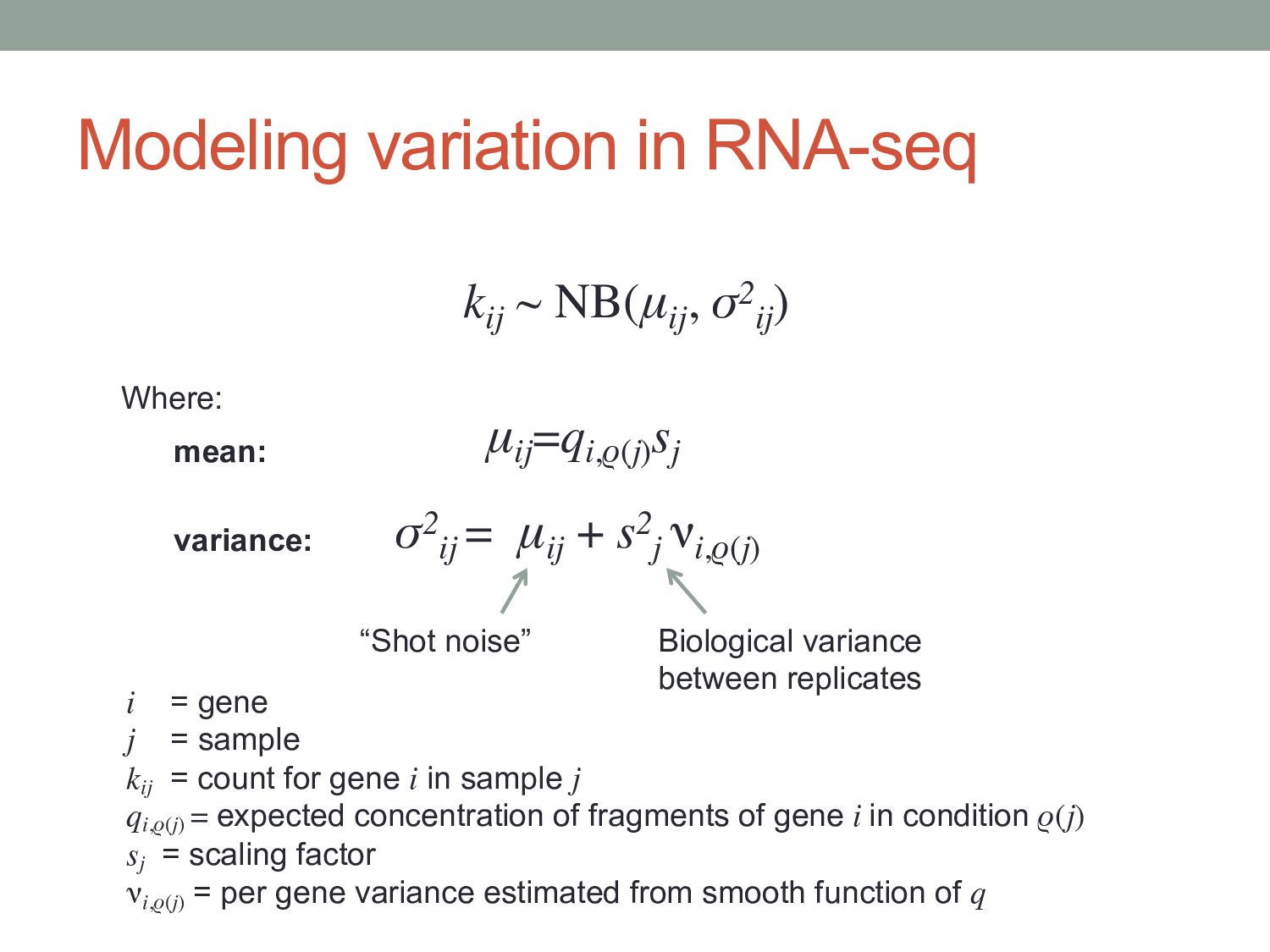
26. Modeling variation in RNA-seq kij ~ NB(μij , σ2 ij ) i = gene j = sample kij = count for gene i in sample j qi,ρ(j) = expected concentration of fragments of gene i in condition ρ(j) sj = scaling factor νi,ρ(j) = per gene variance estimated from smooth function of q Where: μij =qi,ρ(j) sj σ2 ij = μij + s2 j νi,ρ(j) “Shot noise” Biological variance between replicates mean: variance:
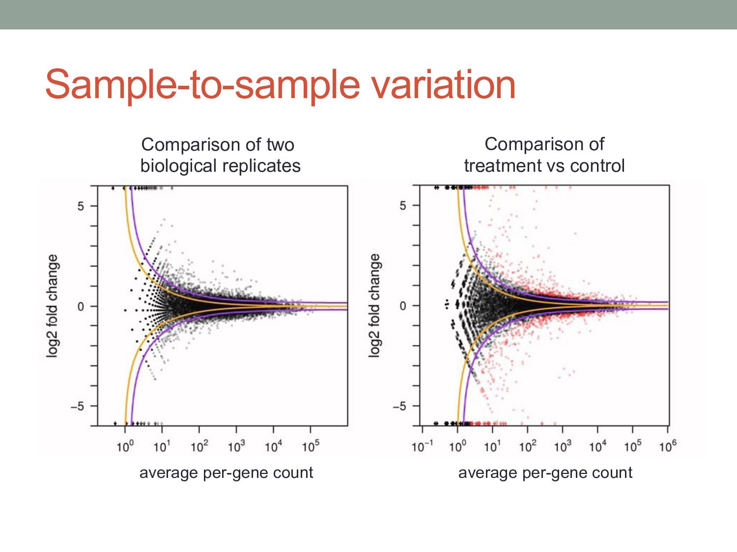
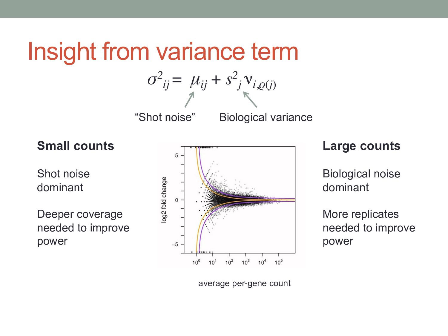
27. Insight from variance term average per-gene count σ2 ij = μij + s2 j νi,ρ(j) “Shot noise” Biological variance Small counts Shot noise dominant Deeper coverage needed to improve power Large counts Biological noise dominant More replicates needed to improve power
28. Sharing estimates of dispersion across genes
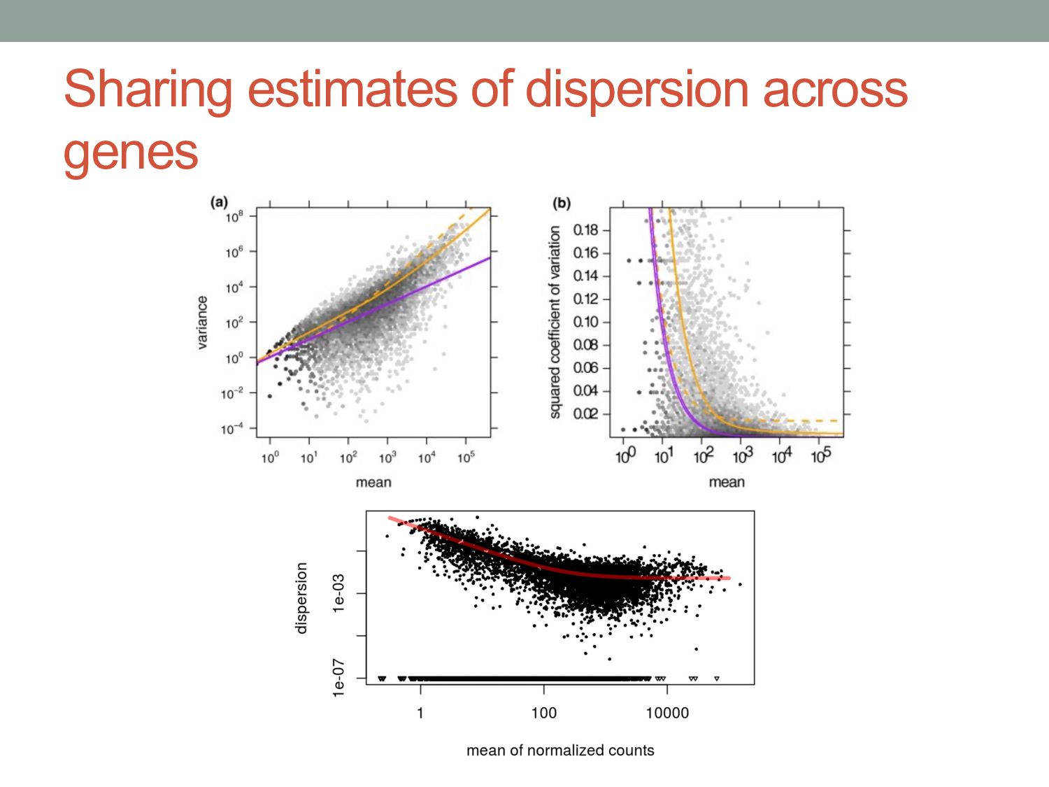
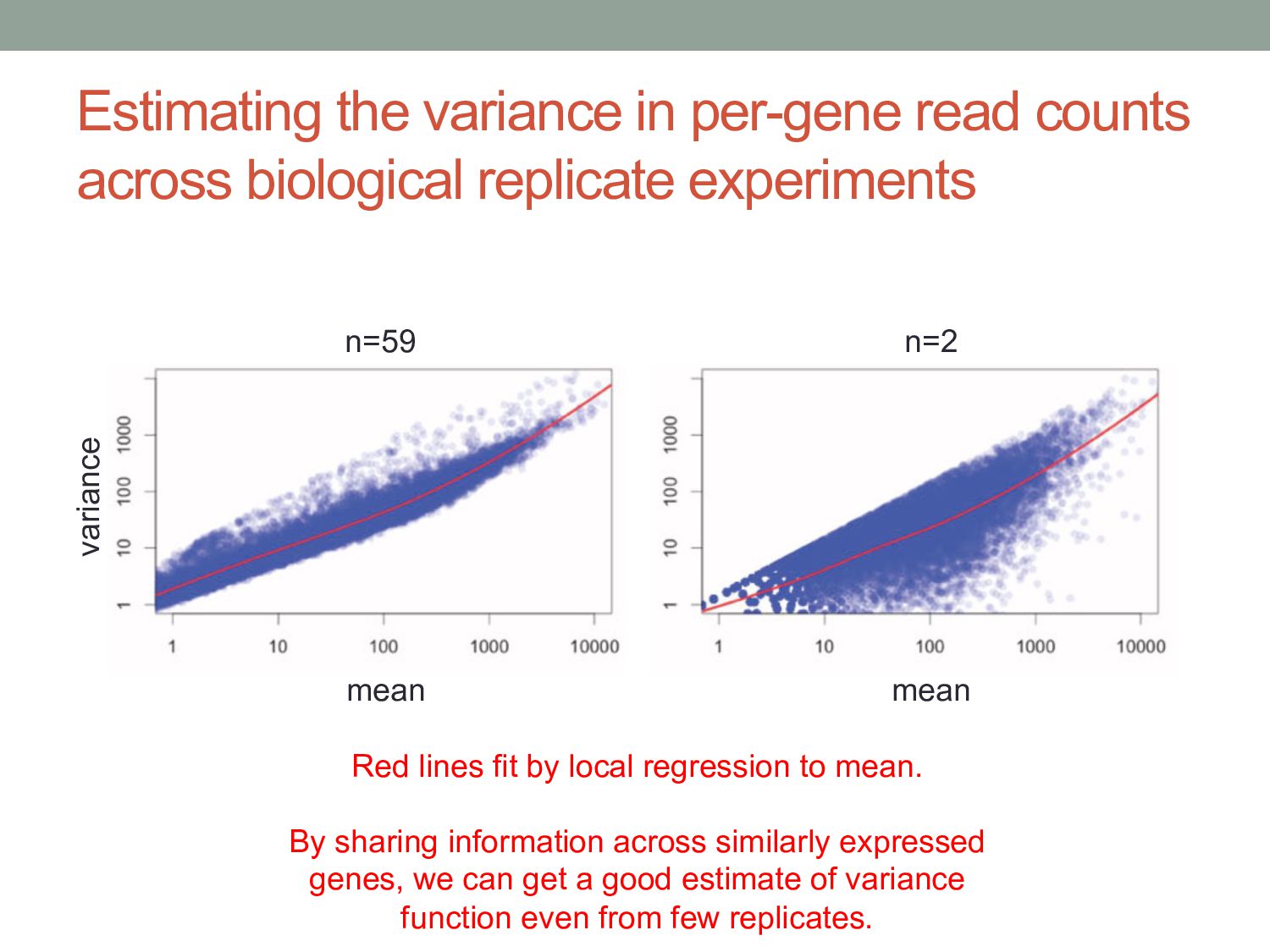
29. Estimating the variance in per-gene read counts across biological replicate experiments n=59 n=2 mean mean variance Red lines fit by local regression to mean. By sharing information across similarly expressed genes, we can get a good estimate of variance function even from few replicates.
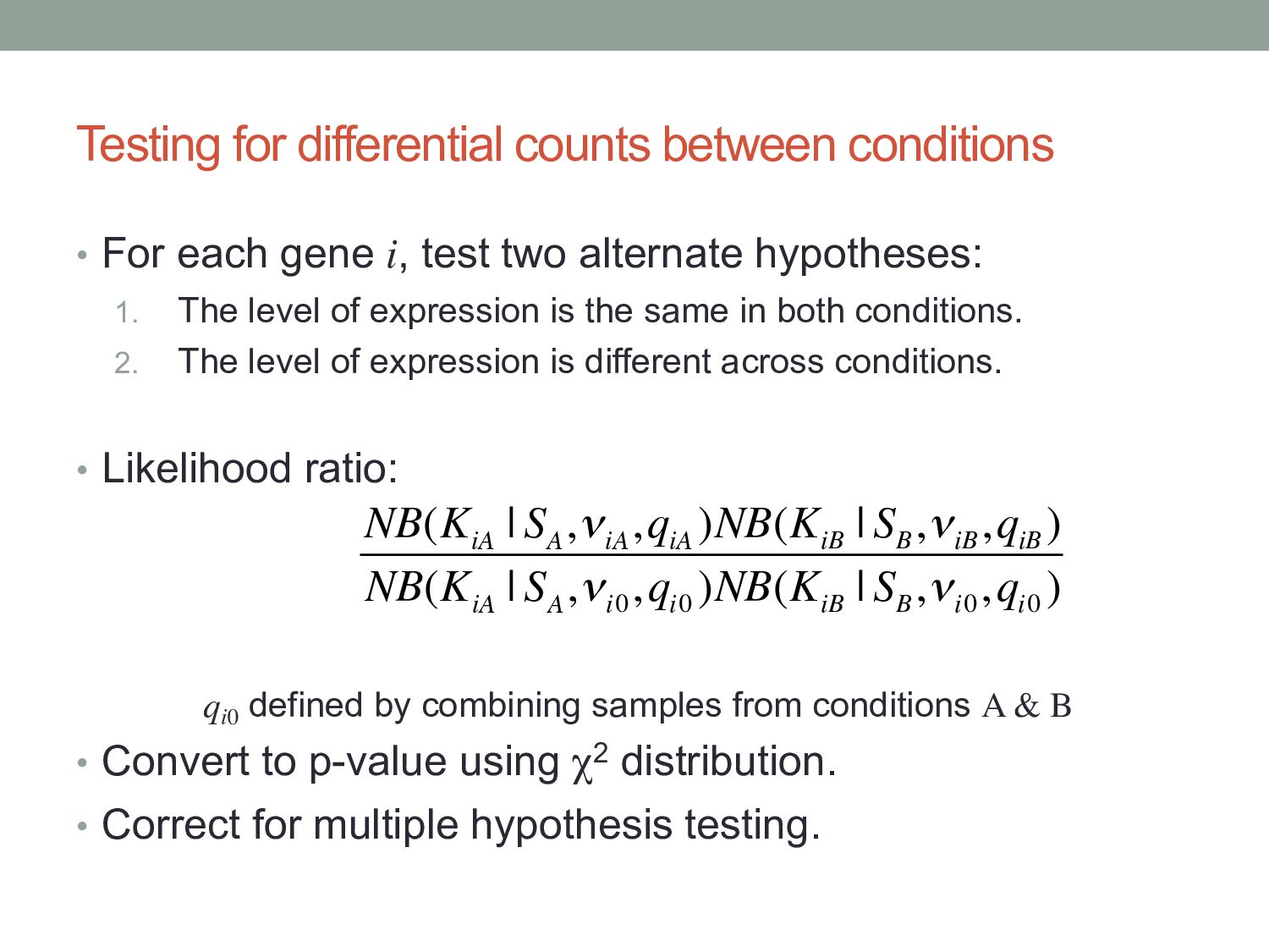
30. Testing for differential counts between conditions • For each gene i, test two alternate hypotheses: 1. The level of expression is the same in both conditions. 2. The level of expression is different across conditions. • Likelihood ratio: qi0 defined by combining samples from conditions A & B • Convert to p-value using χ2 distribution. • Correct for multiple hypothesis testing. NB(K iA | S A ,νiA ,q iA )NB(K iB | S B ,νiB ,q iB ) NB(K iA | S A ,νi0 ,q i0 )NB(K iB | S B ,νi0 ,q i0 )
31. Modeling count data: ANOVA • ANOVA = analysis of variance • Analysis task: are ai & bi significantly different? • Observed read count is a noisy measurement of the mean read count expected in a given condition. • The expected mean count depends on the number of mRNA fragments in that condition and the normalization scaling factors.
32. Significance cut-off for determining differential counts average per-gene count Comparison of two biological replicates Comparison of two treatment vs control average per-gene count
33. RNA-seq reads that span exon-exon junctions will not map directly to the genome To align reads across introns, we need splicing-aware alignment methods
34. How do we map to exon-exon boundaries?
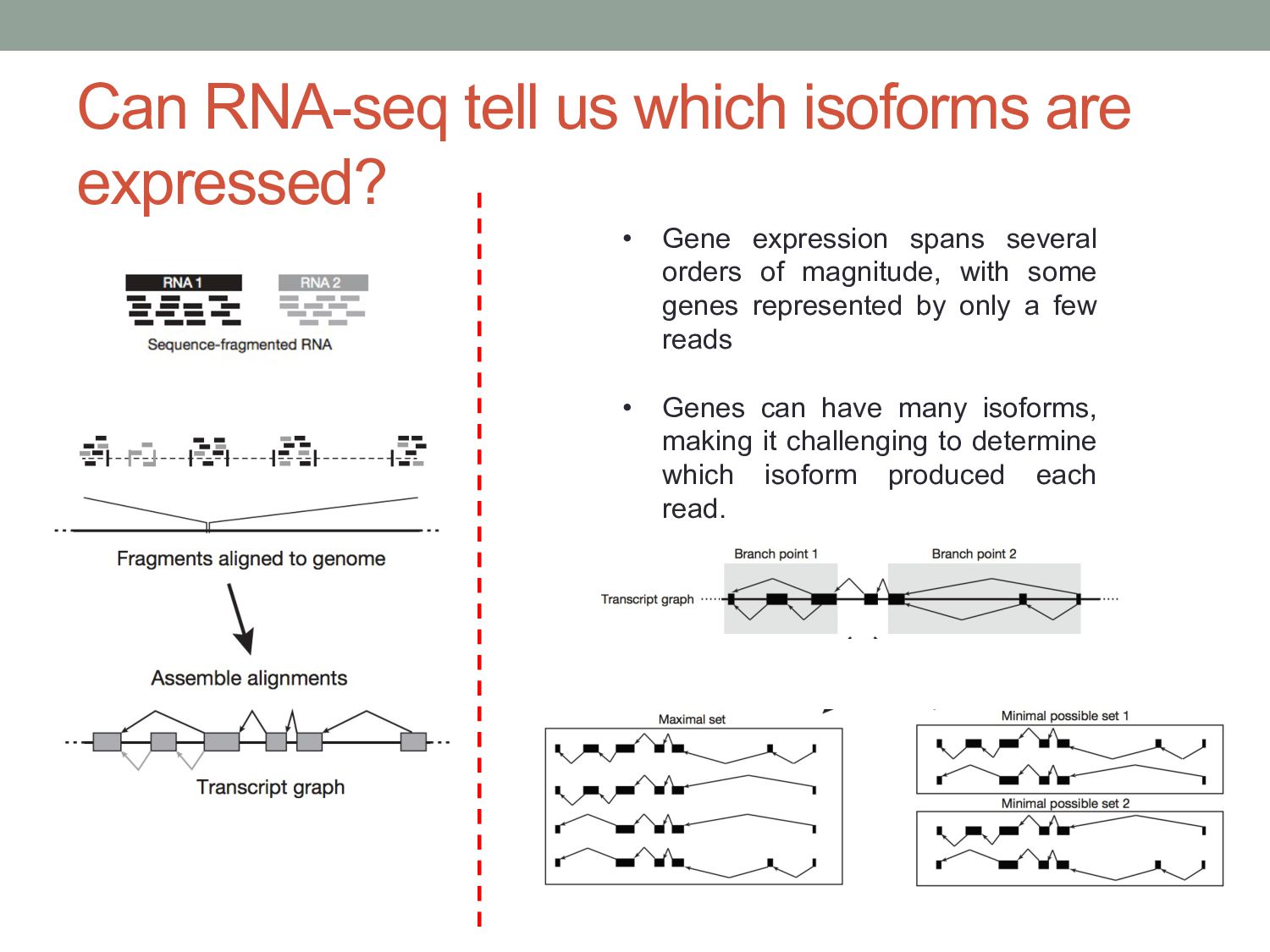
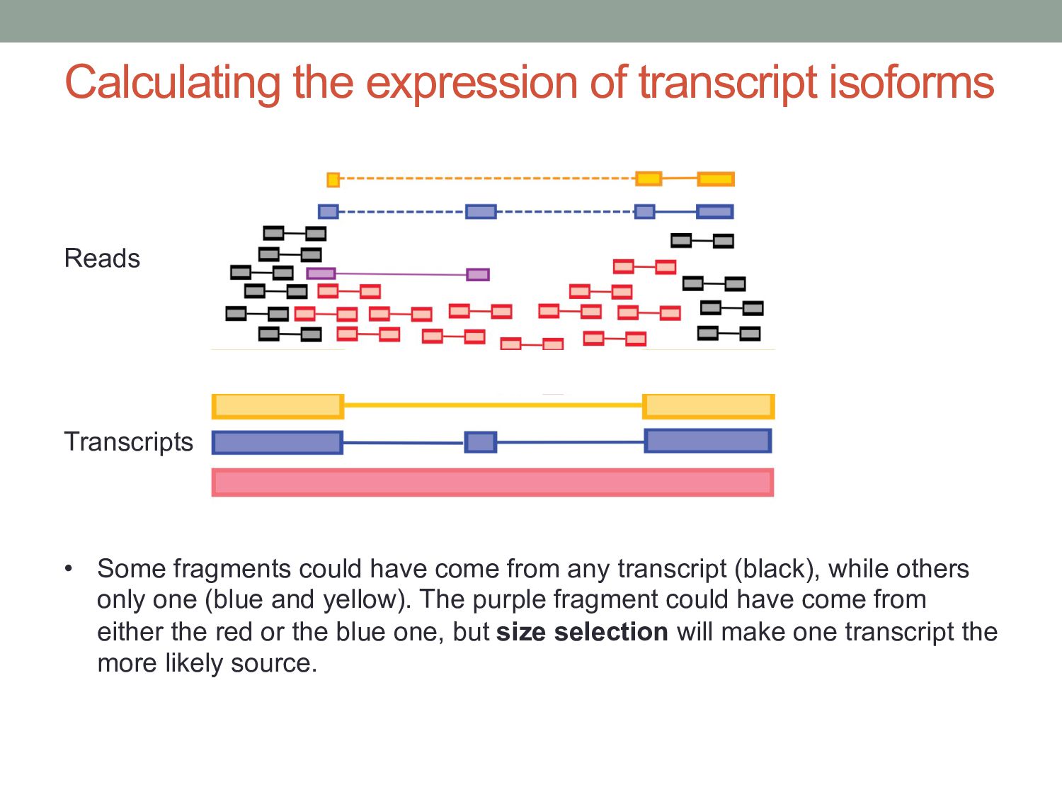
35. • Gene expression spans several orders of magnitude, with some genes represented by only a few reads • Genes can have many isoforms, making it challenging to determine which isoform produced each read. Can RNA-seq tell us which isoforms are expressed?
36. Calculating the expression of transcript isoforms Reads Transcripts
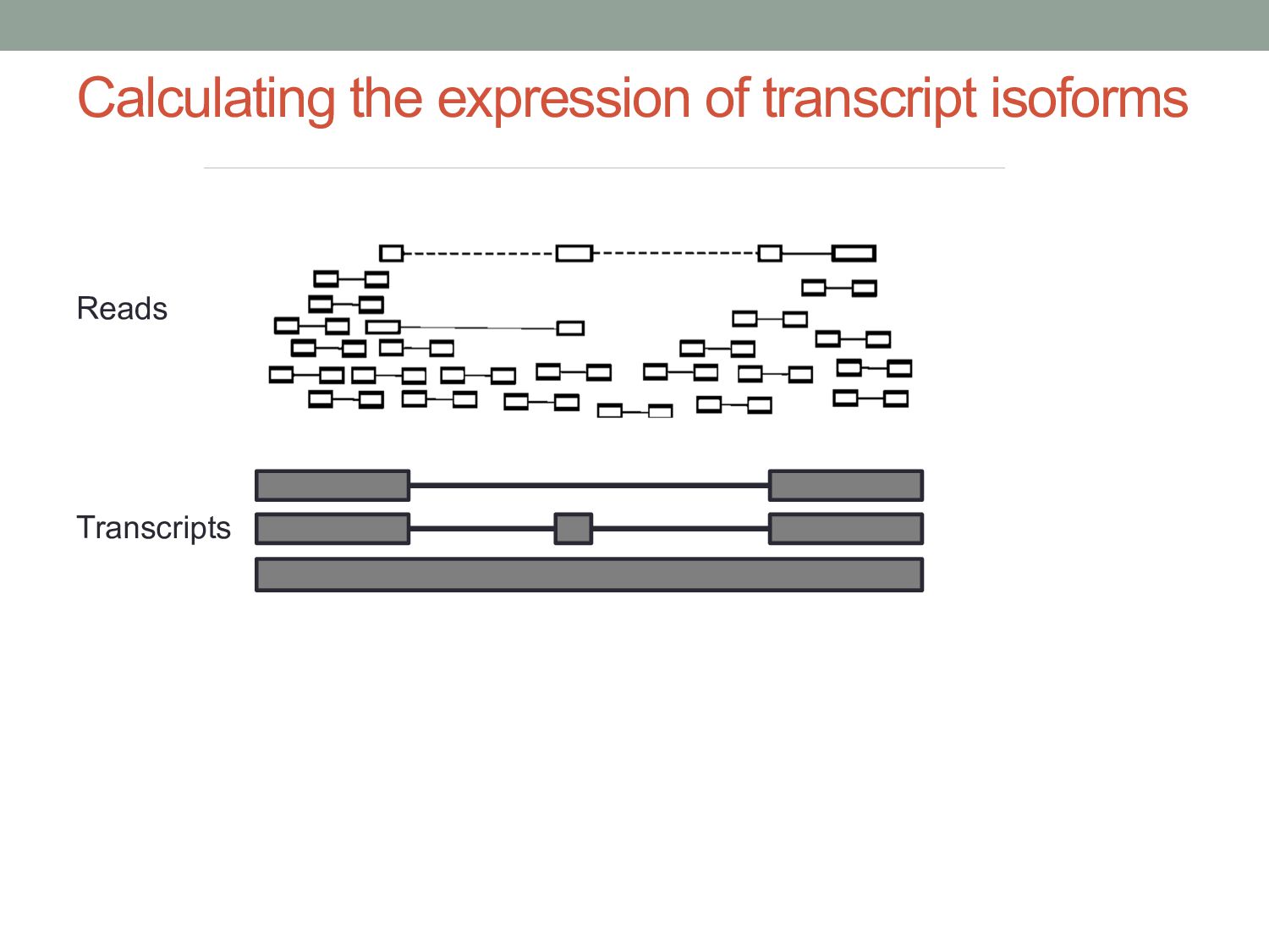
37. Calculating the expression of transcript isoforms • Some fragments could have come from any transcript (black), while others only one (blue and yellow). The purple fragment could have come from either the red or the blue one, but size selection will make one transcript the more likely source. Reads Transcripts
38. Transcript assembly without a reference
39. RNA-seq tutorial • https://training.galaxyproject.org/training- material/topics/transcriptomics/tutorials/rb- rnaseq/tutorial.html
40. Summary • We’re often interested in discovering how biochemical activities vary across cell types or conditions. With functional genomics assays, this involves analyzing differences in read count information. • Statistical analysis of sequencing (count-based) data needs to account for many sources of variance. • Differentially expressed genes can be found using statistical tests based on the Negative Binomial distribution.