Lecture 20 ChIP-seq

BMMB 554 Lecture 20

Transcript

1. L20: CHIP-SEQ Foundations in Data Driven Life Sciences BMMB/MCIBS 554
2. HOW DO TFS FIND THEIR BINDING SITES?
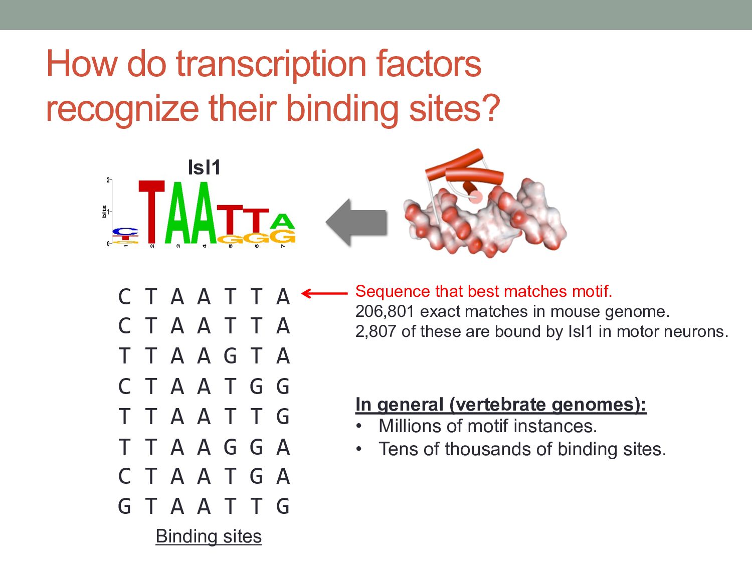
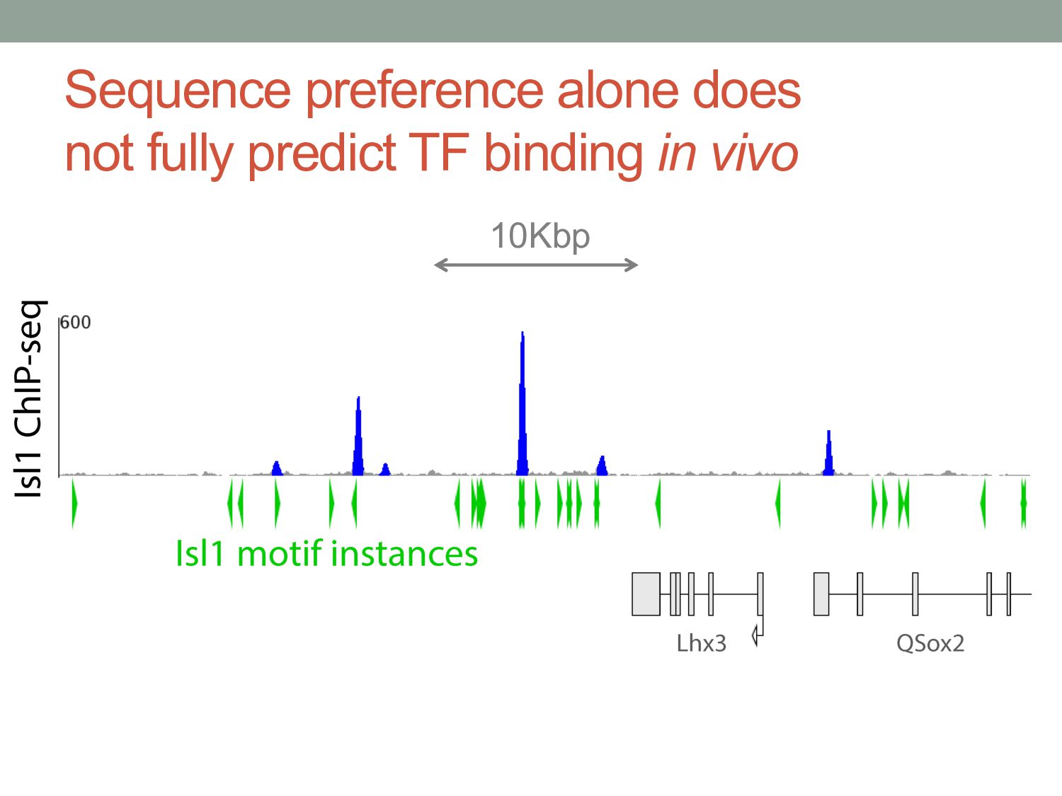
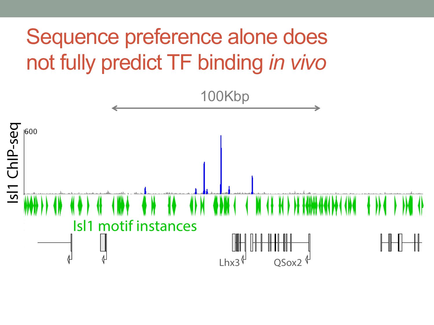
3. How do transcription factors recognize their binding sites? C T A A T T A C T A A T T A T T A A G T A C T A A T G G T T A A T T G T T A A G G A C T A A T G A G T A A T T G Binding sites Sequence that best matches motif. 206,801 exact matches in mouse genome. 2,807 of these are bound by Isl1 in motor neurons. In general (vertebrate genomes): • Millions of motif instances. • Tens of thousands of binding sites. Isl1
4. 10Kbp Sequence preference alone does not fully predict TF binding in vivo
5. 10Kbp Sequence preference alone does not fully predict TF binding in vivo
6. 100Kbp Sequence preference alone does not fully predict TF binding in vivo
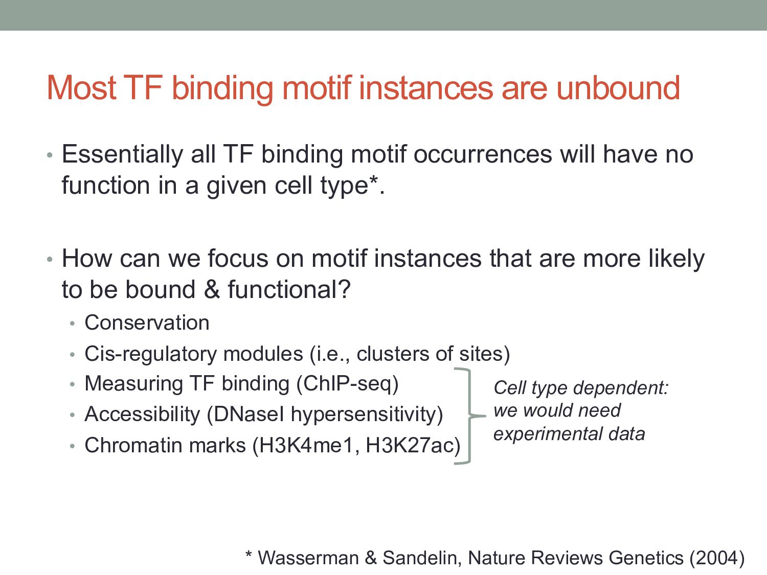
7. Most TF binding motif instances are unbound • Essentially all TF binding motif occurrences will have no function in a given cell type*. • How can we focus on motif instances that are more likely to be bound & functional? • Conservation • Cis-regulatory modules (i.e., clusters of sites) • Measuring TF binding (ChIP-seq) • Accessibility (DNaseI hypersensitivity) • Chromatin marks (H3K4me1, H3K27ac) * Wasserman & Sandelin, Nature Reviews Genetics (2004) Cell type dependent: we would need experimental data
8. Phylogenetic footprinting • Conserved sequences are more likely to be functional.
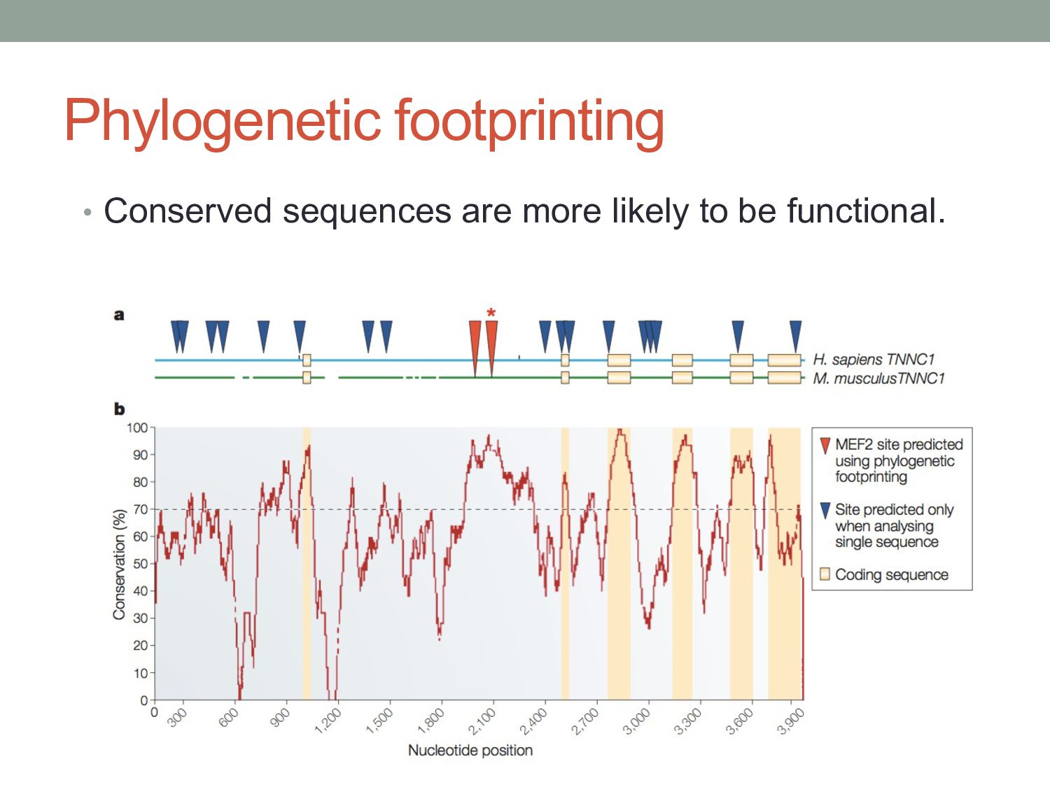
9. Limitations of phylogenetic footprinting • Only ~60% of TF binding sites are directly conserved between human & mouse. • Perhaps even fewer TF binding sites are functionally conserved. • Phylogenetic shadowing approaches allows conservation analysis of binding sites across more closely related species.
10. Cis-regulatory modules • Idea: motif instances should be clustered at real enhancers. • Different combinations of TFs may have different regulatory effects. Regulatory synergy
11. Regulatory regions consist of cooperatively bound TFs
12. Cis-regulatory modules • Multiple TF binding sites will form a stronger binding region. • Motif instances for cooperating TFs should be located together.
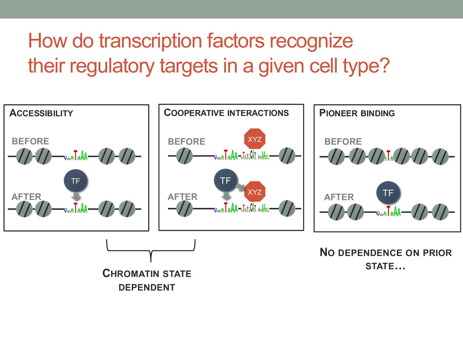
13. How do transcription factors recognize their regulatory targets in a given cell type? CHROMATIN STATE DEPENDENT ACCESSIBILITY TF XYZ COOPERATIVE INTERACTIONS TF XYZ PIONEER BINDING TF BEFORE AFTER BEFORE AFTER BEFORE AFTER NO DEPENDENCE ON PRIOR STATE…
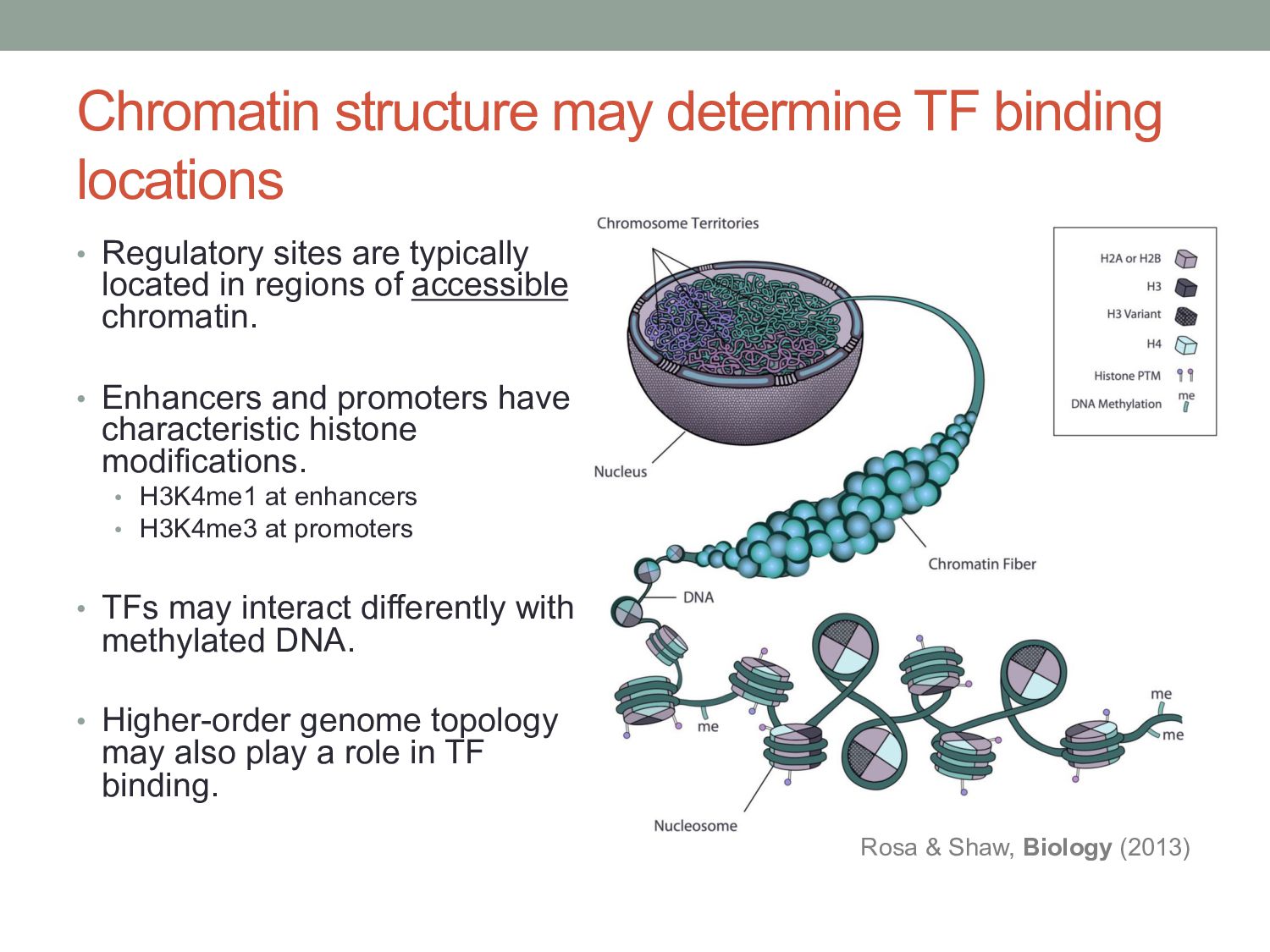
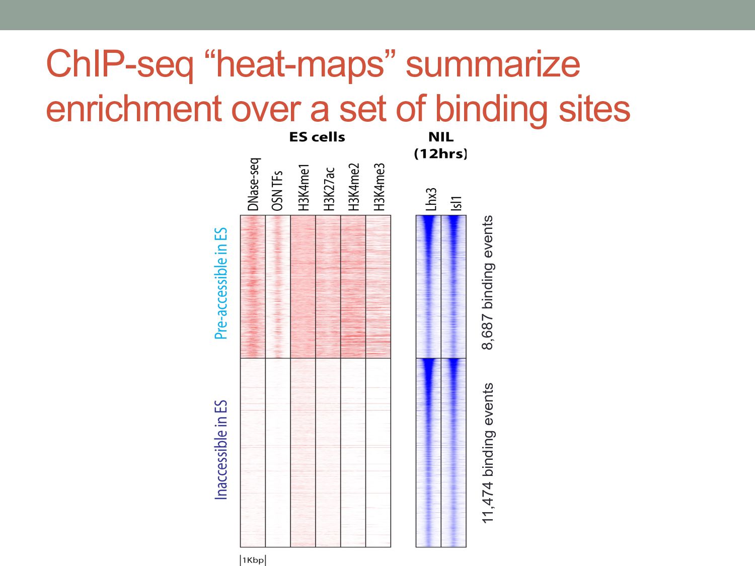
14. Chromatin structure may determine TF binding locations • Regulatory sites are typically located in regions of accessible chromatin. • Enhancers and promoters have characteristic histone modifications. • H3K4me1 at enhancers • H3K4me3 at promoters • TFs may interact differently with methylated DNA. • Higher-order genome topology may also play a role in TF binding. Rosa & Shaw, Biology (2013)
15. PROTEIN-DNA BINDING ASSAYS
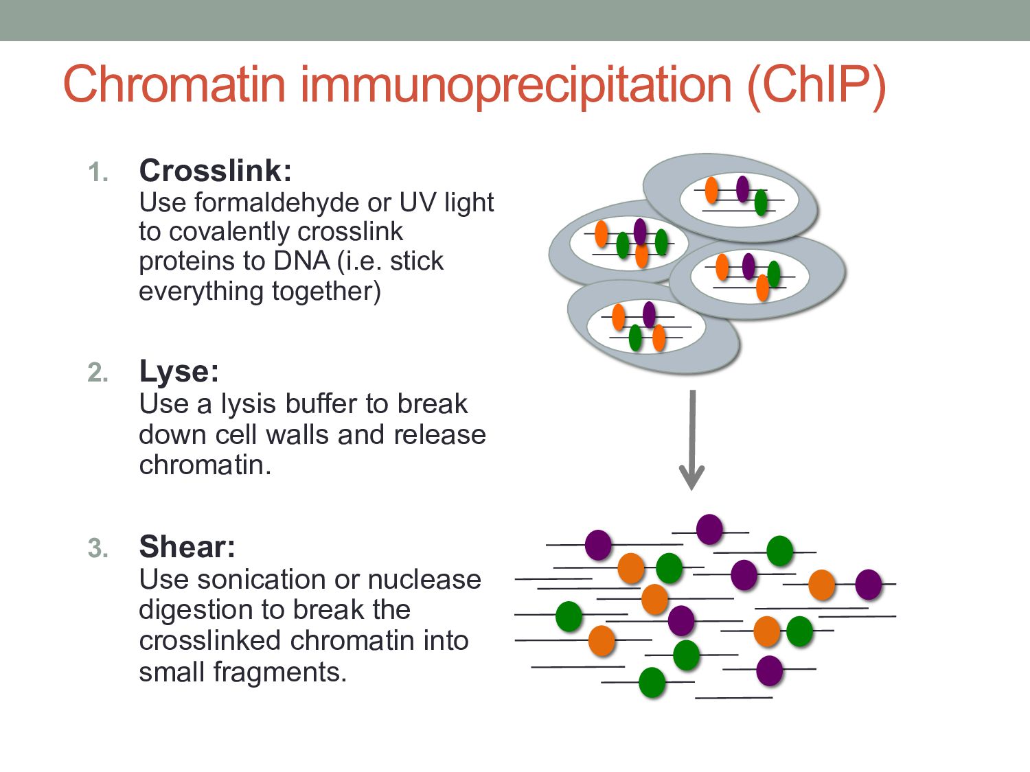
16. Chromatin immunoprecipitation (ChIP) 1. Crosslink: Use formaldehyde or UV light to covalently crosslink proteins to DNA (i.e. stick everything together) 2. Lyse: Use a lysis buffer to break down cell walls and release chromatin. 3. Shear: Use sonication or nuclease digestion to break the crosslinked chromatin into small fragments.
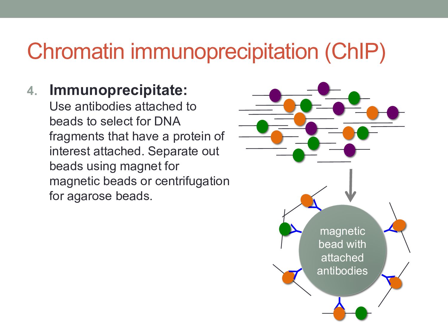
17. Chromatin immunoprecipitation (ChIP) 4. Immunoprecipitate: Use antibodies attached to beads to select for DNA fragments that have a protein of interest attached. Separate out beads using magnet for magnetic beads or centrifugation for agarose beads. Y Y Y Y Y magnetic bead with attached antibodies Y
18. Chromatin immunoprecipitation (ChIP) 5. Reverse crosslinks Incubate at 70°C to reverse cross-linking (i.e., unstick DNA from protein), and separate DNA.
19. Chromatin immunoprecipitation (ChIP) 6. Library preparation: Select DNA fragments that are ~200bp in length. Amplify the fragments using PCR. Size select PCR amplify
20. ChIP-seq • Directly sequence ChIPed DNA fragments using a high-throughput sequencer. • Sequence one or both fragment ends? • à FASTQ file • Map the sequenced reads back to the genome. • Bowtie / BWA • à BAM file
21. ChIP-exo provides higher resolution
22. Other protein-DNA binding assays
23. Using MNase to find protein-DNA interactions
24. VISUALIZING CHIP-SEQ DATA
25. Data smoothing helps ChIP-seq signals to stand out + - 500bp Foxa2 Liver ChIP-seq Aldh1a1 ~35Kbp upstream
26. Data smoothing helps ChIP-seq signals to stand out + - 500bp Foxa2 Liver ChIP-seq extend in 3’ direction Aldh1a1 ~35Kbp upstream
27. Data smoothing helps ChIP-seq signals to stand out + - 500bp Foxa2 Liver ChIP-seq extend in 3’ direction remove strandedness Aldh1a1 ~35Kbp upstream
28. Making genome browser tracks • Why view data in a browser? • Visually assess quality of ChIP-enrichment • Confirm previously known binding targets • Explore the data! • Genome browsers • UCSC genome browser (tracks from Galaxy) [http://genome.ucsc.edu] • IGV [https://www.broadinstitute.org/igv]
29. ChIP-seq “heat-maps” summarize enrichment over a set of binding sites Site 1 Site 2 Site 3 Site N 1Kbp
30. ChIP-seq “heat-maps” summarize enrichment over a set of binding sites 11,474 binding events 8,687 binding events
31. FINDING TF BINDING EVENTS IN CHIP-SEQ DATA
32. ChIP-seq ChIP-seq signal can be punctate or broadly distributed (or both) Park, Nature Reviews Genetics (2009)
33. ChIP-seq ChIP-seq experiments vary in efficiency
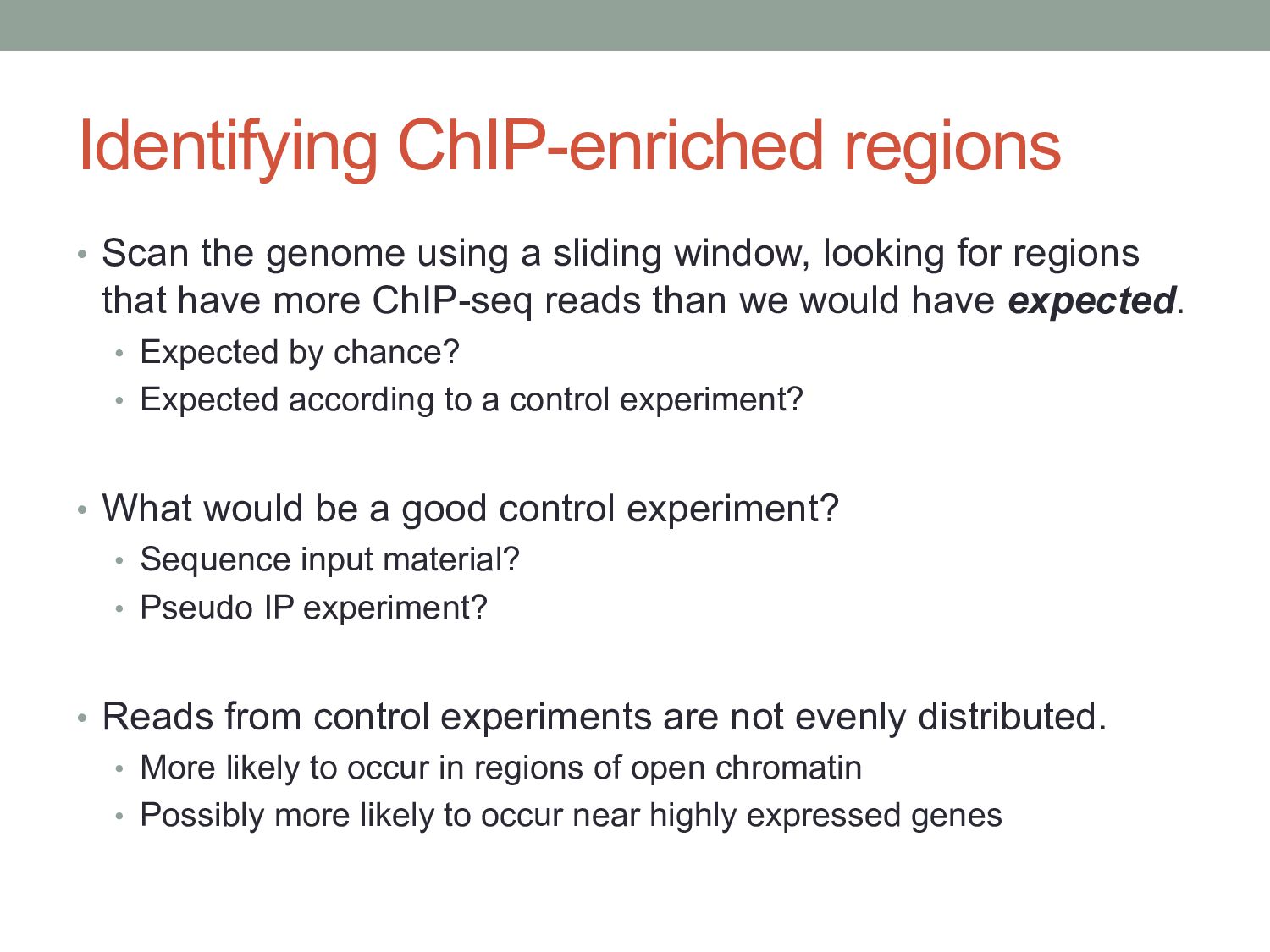
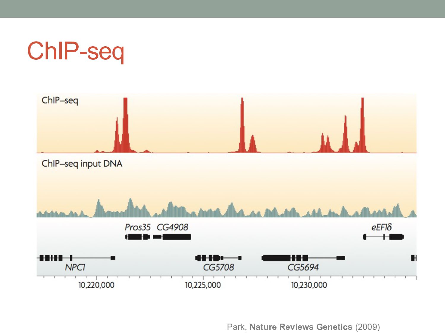
34. Identifying ChIP-enriched regions • Scan the genome using a sliding window, looking for regions that have more ChIP-seq reads than we would have expected. • Expected by chance? • Expected according to a control experiment? • What would be a good control experiment? • Sequence input material? • Pseudo IP experiment? • Reads from control experiments are not evenly distributed. • More likely to occur in regions of open chromatin • Possibly more likely to occur near highly expressed genes
35. ChIP-seq Park, Nature Reviews Genetics (2009)
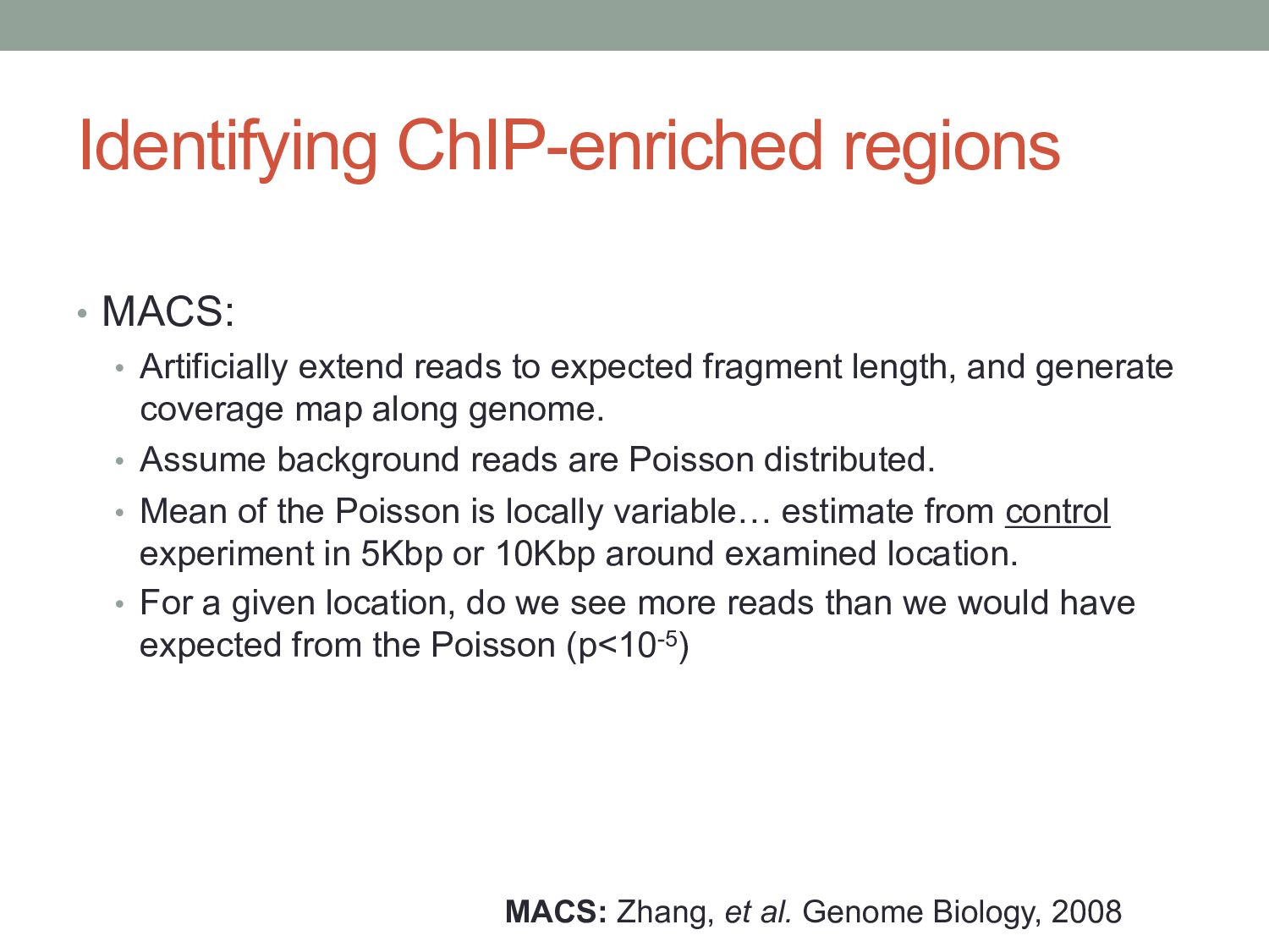
36. Identifying ChIP-enriched regions • MACS: • Artificially extend reads to expected fragment length, and generate coverage map along genome. • Assume background reads are Poisson distributed. • Mean of the Poisson is locally variable… estimate from control experiment in 5Kbp or 10Kbp around examined location. • For a given location, do we see more reads than we would have expected from the Poisson (p<10-5) MACS: Zhang, et al. Genome Biology, 2008
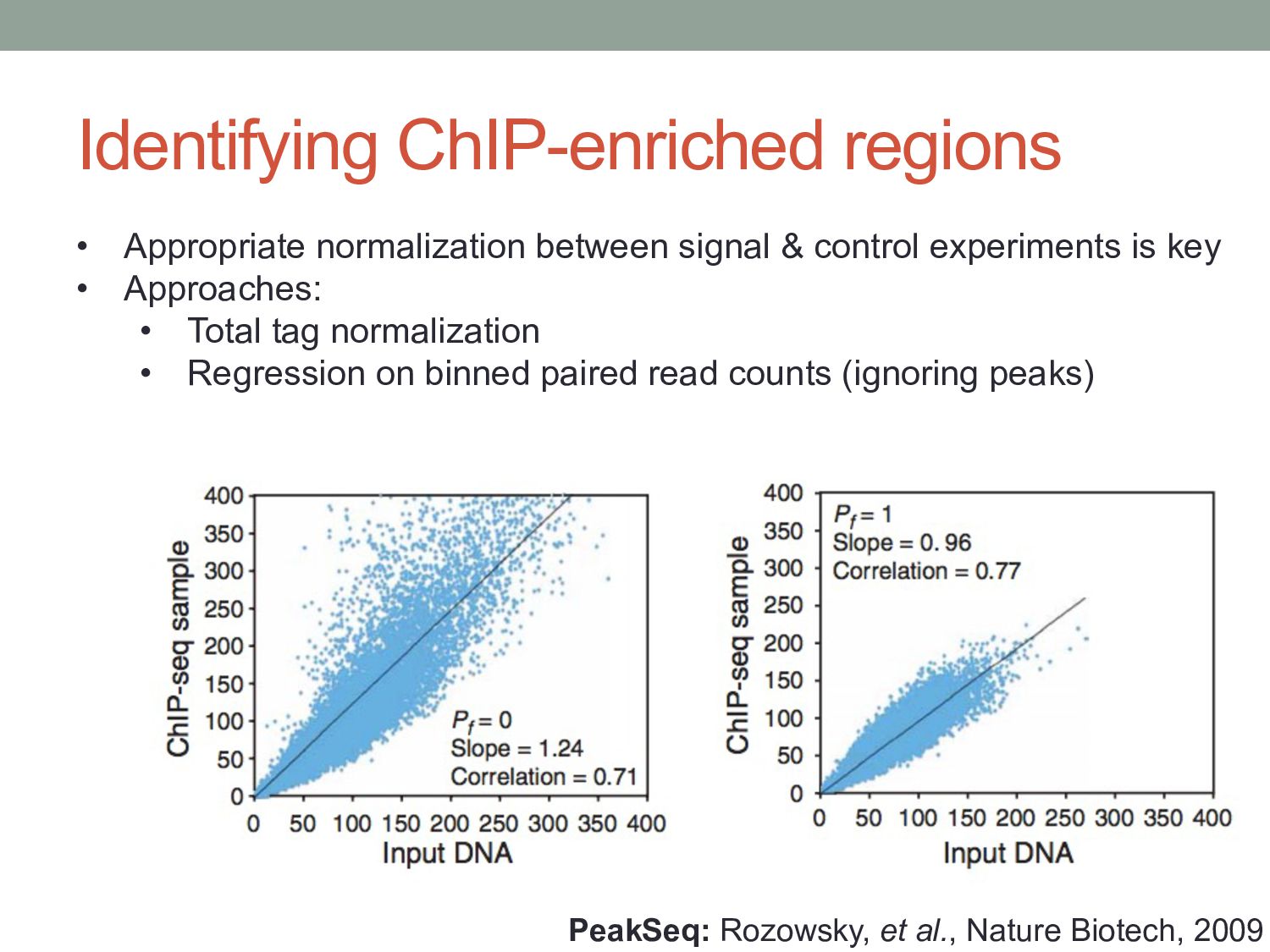
37. Identifying ChIP-enriched regions PeakSeq: Rozowsky, et al., Nature Biotech, 2009 • Appropriate normalization between signal & control experiments is key • Approaches: • Total tag normalization • Regression on binned paired read counts (ignoring peaks)
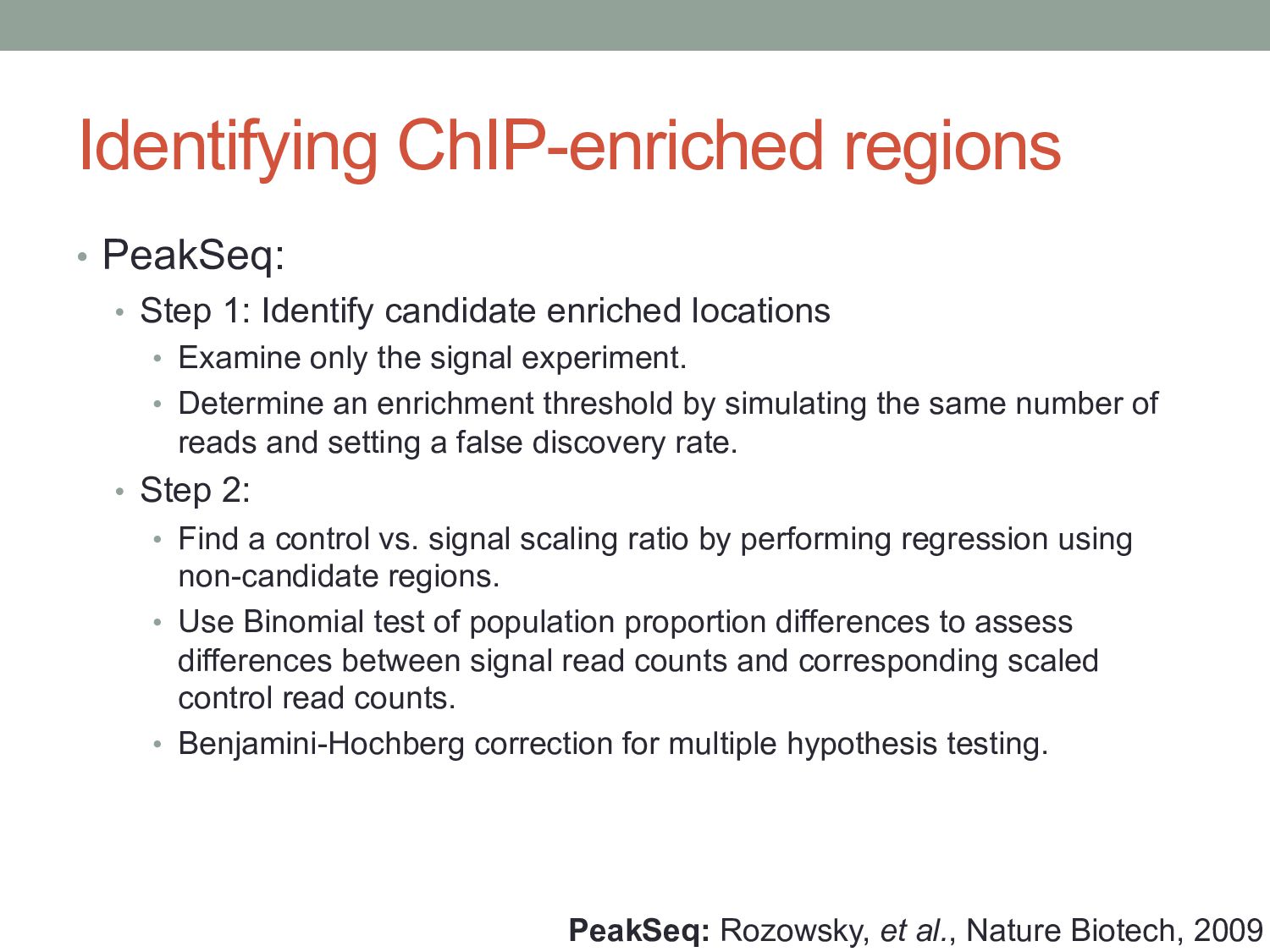
38. Identifying ChIP-enriched regions • PeakSeq: • Step 1: Identify candidate enriched locations • Examine only the signal experiment. • Determine an enrichment threshold by simulating the same number of reads and setting a false discovery rate. • Step 2: • Find a control vs. signal scaling ratio by performing regression using non-candidate regions. • Use Binomial test of population proportion differences to assess differences between signal read counts and corresponding scaled control read counts. • Benjamini-Hochberg correction for multiple hypothesis testing. PeakSeq: Rozowsky, et al., Nature Biotech, 2009
39. How many locations does a protein bind? • Statistical answers: • p-value thresholds (significance of enrichment) • Fold-enrichment cutoffs • Greater sequencing depth typically yields higher numbers of peaks. • Statistical significance vs. biological significance?
40. Identifying precise TF binding locations • ChIP-seq reads are distributed bimodally around binding sites. • Regions of ChIP-enrichment are known as “peaks”. Valouev, et al. Nature Methods (2008)
41. Identifying precise TF binding locations
42. Computational challenge: resolve the structure of TF binding events from ChIP-seq data How many binding events are here? How close to the actual bound bases are event predictions? + -
43. Mixture models of ChIP-seq binding events Lhx3 ChIP-seq
44. Mixture models of ChIP-seq binding events Lhx3 ChIP-seq
45. Mixture models of ChIP-seq binding events Lhx3 ChIP-seq
46. Mixture models of ChIP-seq binding events Lhx3 ChIP-seq Predicted binding events: Motif instances: 140bp 160bp
47. GPS/GEM/ChExMix allow more accurate spatial resolution of binding events GEM: http://groups.csail.mit.edu/cgs/gem/
48. EVALUATING CHIP-SEQ QUALITY
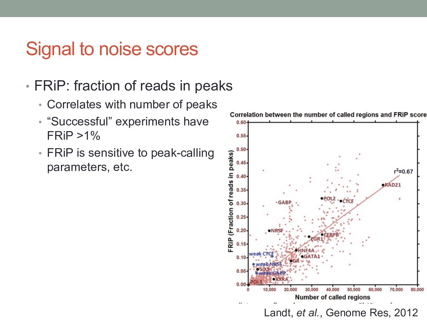
49. Signal to noise scores • FRiP: fraction of reads in peaks • Correlates with number of peaks • “Successful” experiments have FRiP >1% • FRiP is sensitive to peak-calling parameters, etc. Landt, et al., Genome Res, 2012
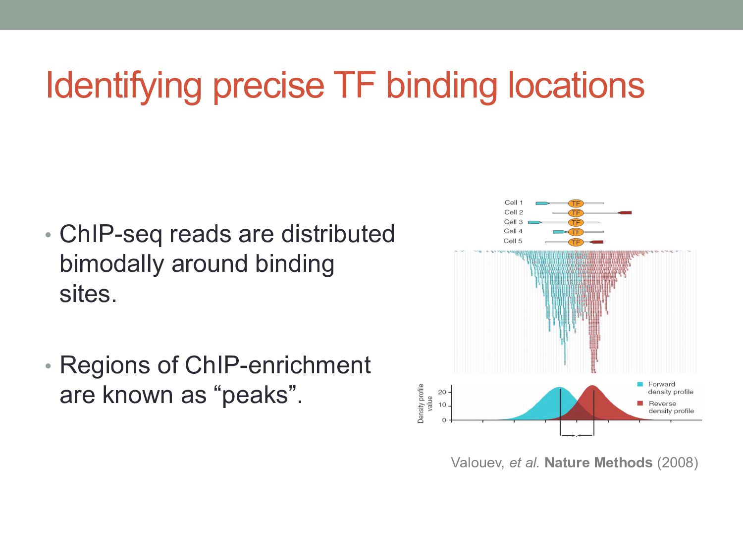
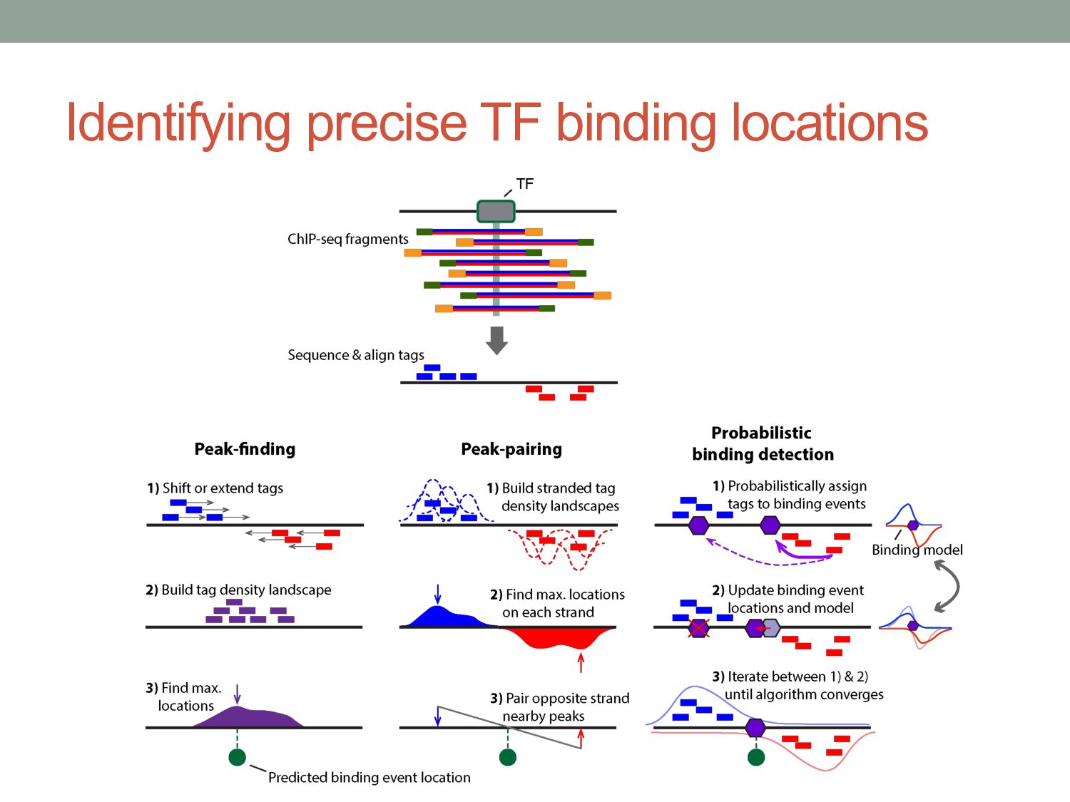
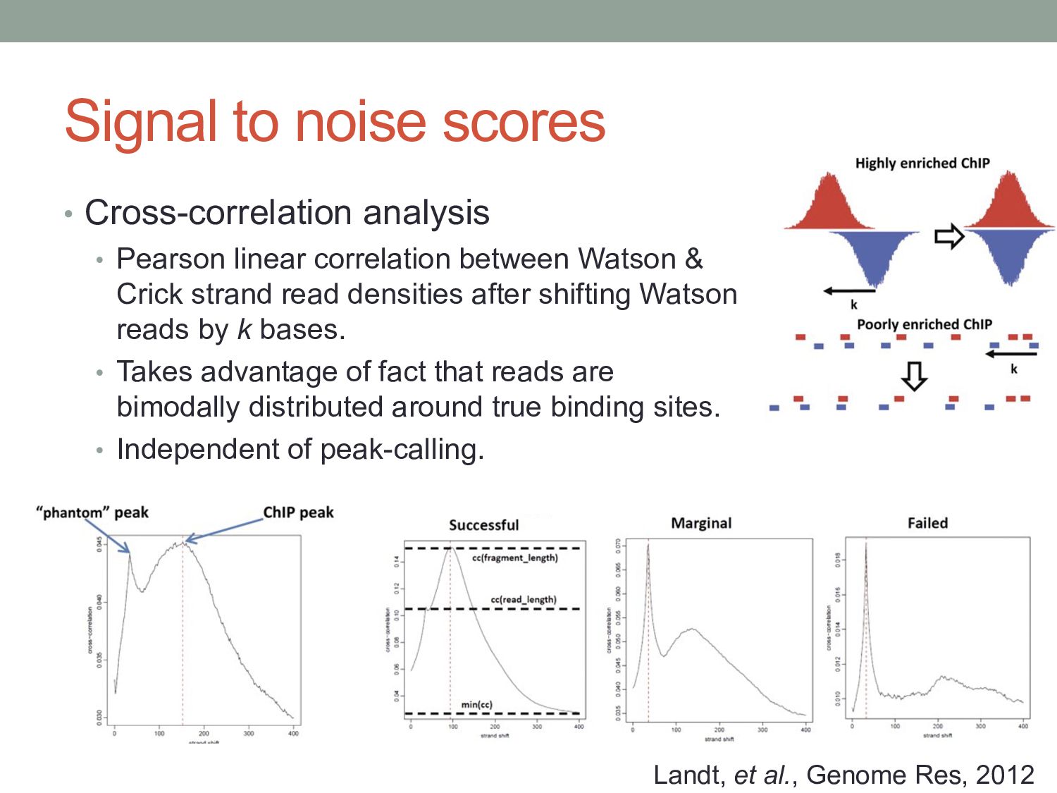
50. Signal to noise scores • Cross-correlation analysis • Pearson linear correlation between Watson & Crick strand read densities after shifting Watson reads by k bases. • Takes advantage of fact that reads are bimodally distributed around true binding sites. • Independent of peak-calling. Landt, et al., Genome Res, 2012
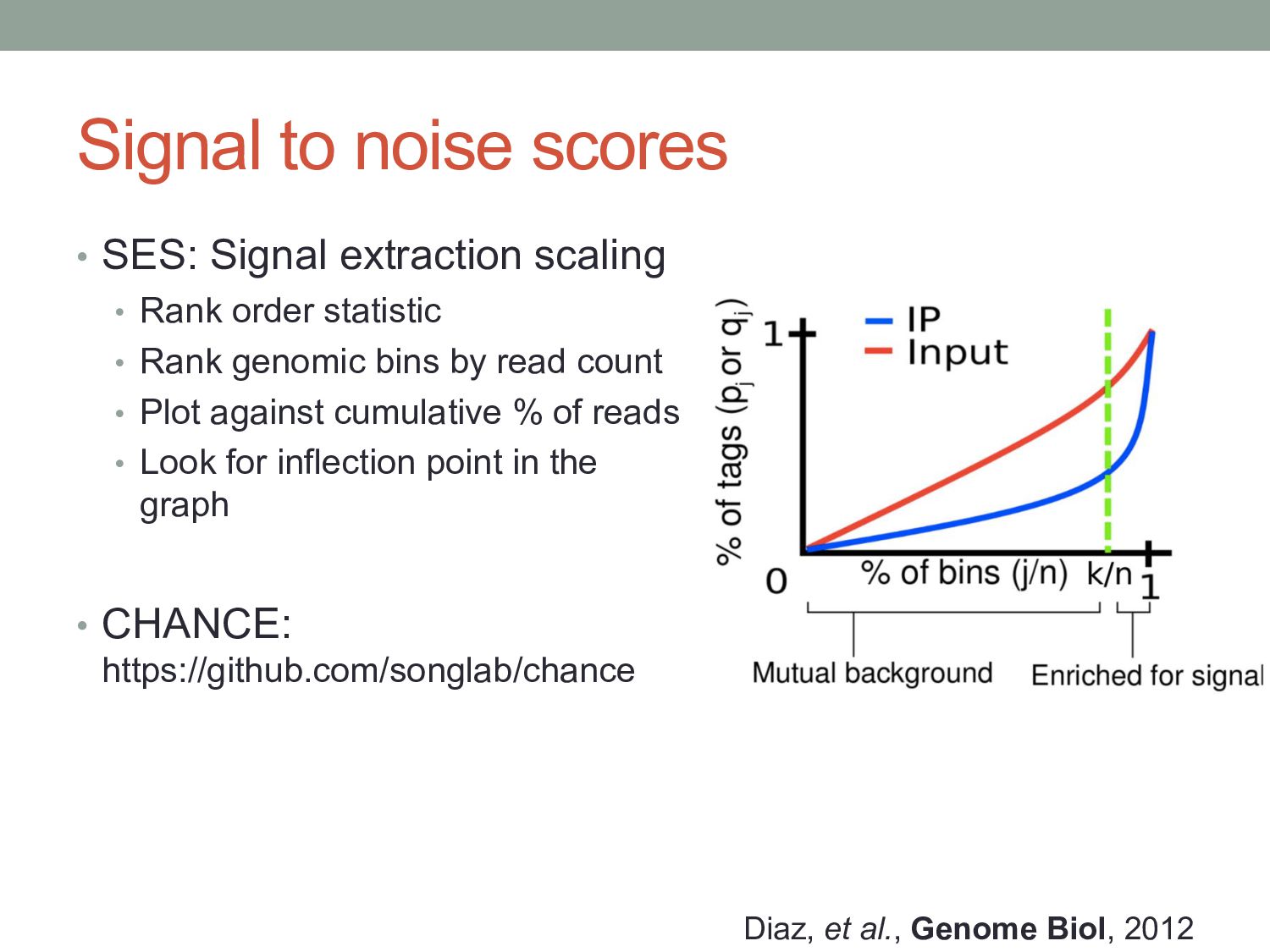
51. Signal to noise scores • SES: Signal extraction scaling • Rank order statistic • Rank genomic bins by read count • Plot against cumulative % of reads • Look for inflection point in the graph • CHANCE: https://github.com/songlab/chance Diaz, et al., Genome Biol, 2012
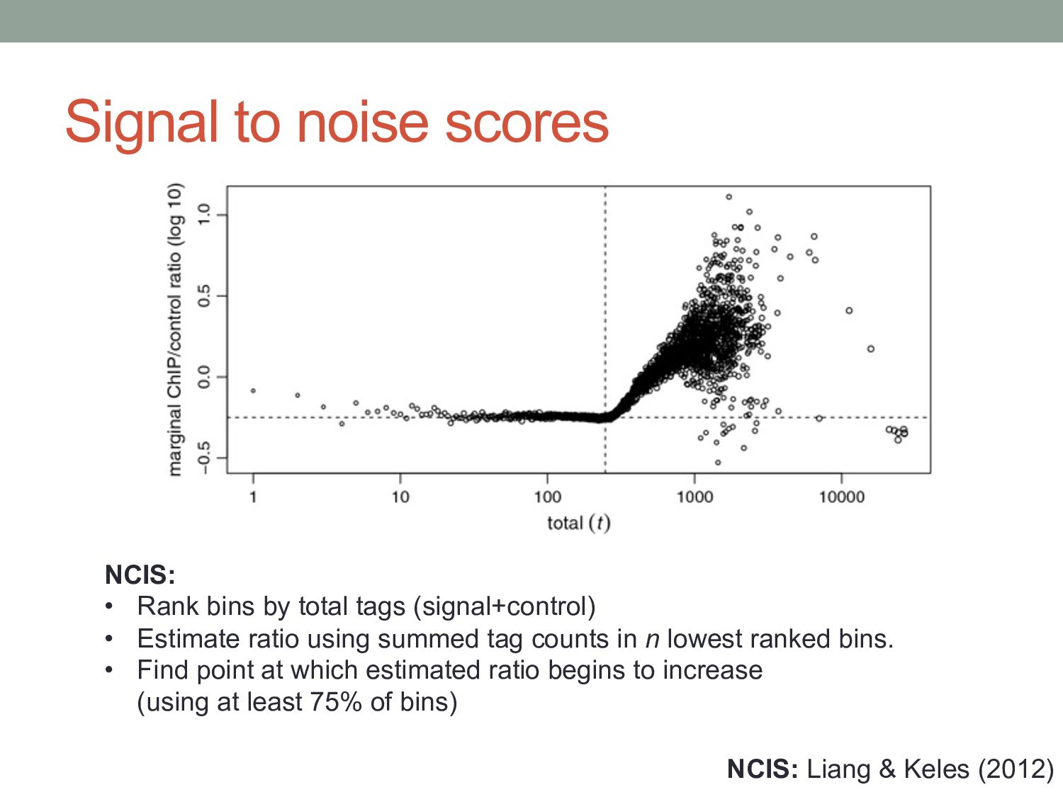
52. Signal to noise scores NCIS: Liang & Keles (2012) NCIS: • Rank bins by total tags (signal+control) • Estimate ratio using summed tag counts in n lowest ranked bins. • Find point at which estimated ratio begins to increase (using at least 75% of bins)
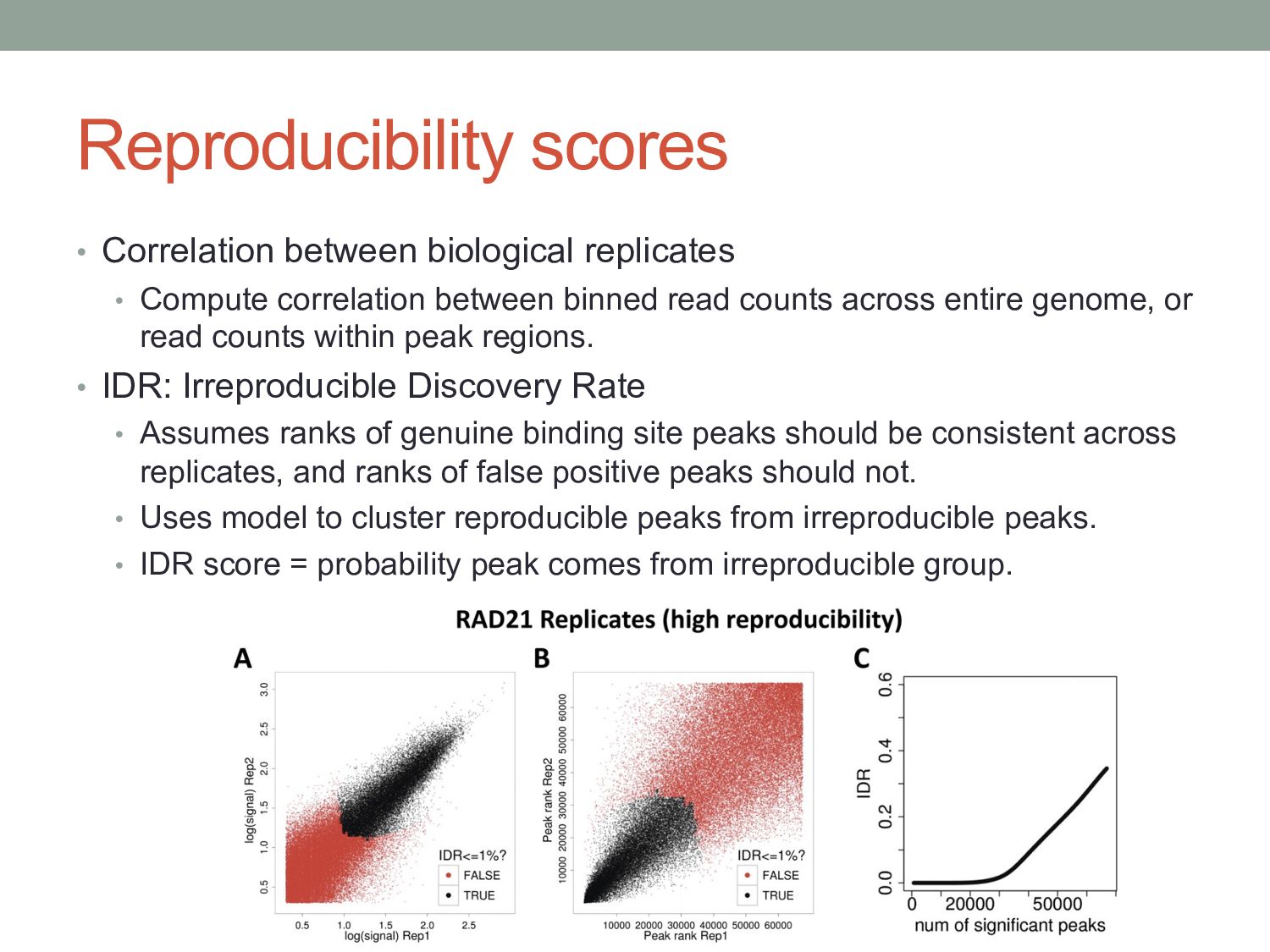
53. Reproducibility scores • Correlation between biological replicates • Compute correlation between binned read counts across entire genome, or read counts within peak regions. • IDR: Irreproducible Discovery Rate • Assumes ranks of genuine binding site peaks should be consistent across replicates, and ranks of false positive peaks should not. • Uses model to cluster reproducible peaks from irreproducible peaks. • IDR score = probability peak comes from irreproducible group.
54. Peak-finders have a wide range of reproducibility Li, et al., Annals of Applied Statistics (2011)
55. Summary • We cannot (yet) predict where a given transcription factor will bind in a given cell type. • Motif scanning yields too many potential sites. • ChIP-seq or other experimental approaches are required. • Analysis of ChIP-seq and other protein-DNA binding assay data is not fully standardized • Choice of peak-finding methodology & interpretation of QC metrics is dataset-dependent. • Many tools available for ChIP-seq analysis, only some of which are accessible beyond the command-line. • Few principled performance comparisons have been performed.
56. Further reading • Park PJ “ChIP-seq: advantages and disadvantages of a maturing technology”, Nature Reviews Genetics (2009) 10(10):669-680 • Landt S, et al. “ChIP-seq guidelines and practices of the ENCODE and modENCODE consortia”, Genome Research (2012) 22:1813 – 1831 • Carroll TS, et al. “Impact of artifact removal on ChIP quality metrics in ChIP-seq and ChIP-exo data”, Frontiers in Genetics (2014) 5:75 • Mahony S & Pugh BF “Protein-DNA binding in high resolution”, Critical Reviews in Biochemistry and Molecular Biology (2015) 4:269-283