lecture 21 motif-finding

BMMB 554 Lecture 21

Transcript

1. L21: MOTIF-FINDING Foundations in Data Driven Life Sciences BMMB 554
2. Learning objectives • Understand the ideas behind the Expectation Maximization machine-learning algorithm. • Learn how this algorithm is applied to discover DNA motifs.
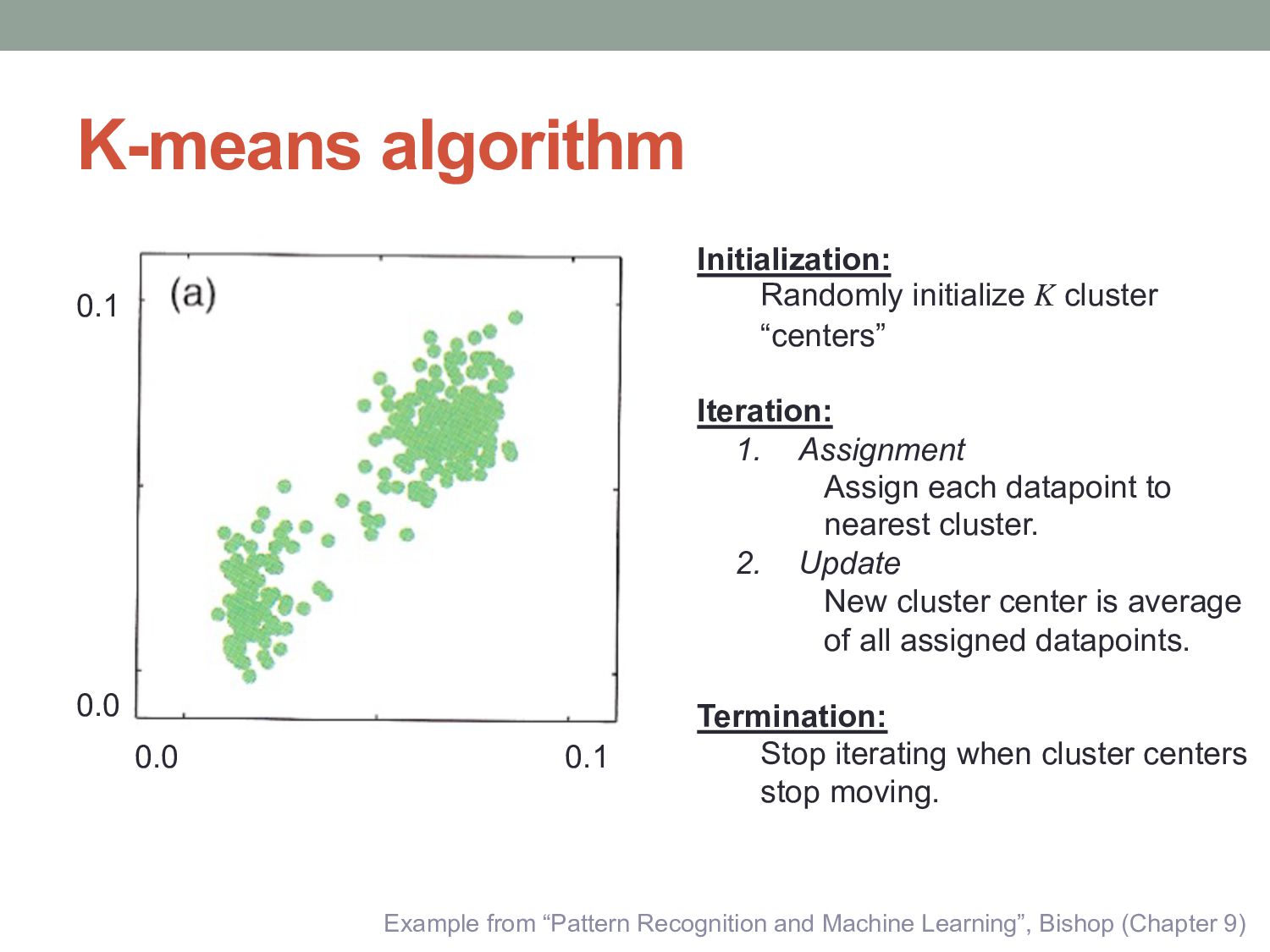
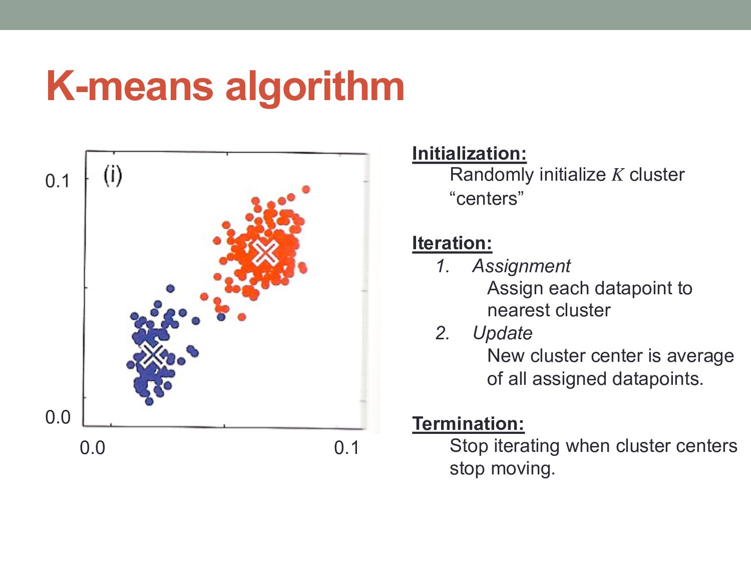
3. K-means algorithm 0.0 0.1 0.1 0.0 Example from “Pattern Recognition and Machine Learning”, Bishop (Chapter 9) Initialization: Randomly initialize K cluster “centers” Iteration: 1. Assignment Assign each datapoint to nearest cluster. 2. Update New cluster center is average of all assigned datapoints. Termination: Stop iterating when cluster centers stop moving.
4. K-means algorithm 0.0 0.1 0.1 0.0 Initialization: Randomly initialize K cluster “centers” Iteration: 1. Assignment Assign each datapoint to nearest cluster 2. Update New cluster center is average of all assigned datapoints. Termination: Stop iterating when cluster centers stop moving.
5. K-means algorithm 0.0 0.1 0.1 0.0 Initialization: Randomly initialize K cluster “centers” Iteration: 1. Assignment Assign each datapoint to nearest cluster 2. Update New cluster center is average of all assigned datapoints. Termination: Stop iterating when cluster centers stop moving.
6. K-means algorithm 0.0 0.1 0.1 0.0 Initialization: Randomly initialize K cluster “centers” Iteration: 1. Assignment Assign each datapoint to nearest cluster 2. Update New cluster center is average of all assigned datapoints. Termination: Stop iterating when cluster centers stop moving.
7. K-means algorithm 0.0 0.1 0.1 0.0 Initialization: Randomly initialize K cluster “centers” Iteration: 1. Assignment Assign each datapoint to nearest cluster 2. Update New cluster center is average of all assigned datapoints. Termination: Stop iterating when cluster centers stop moving.
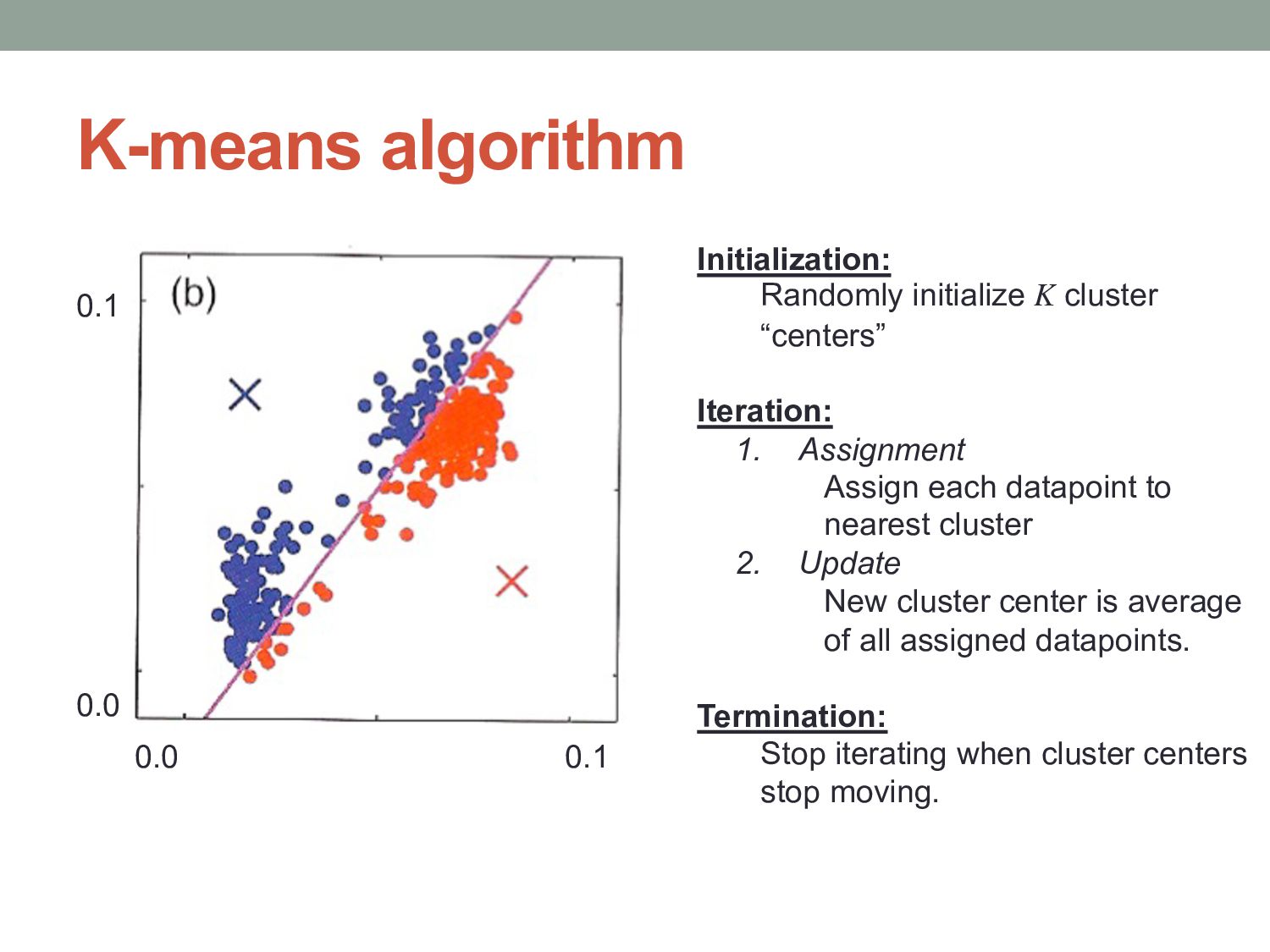
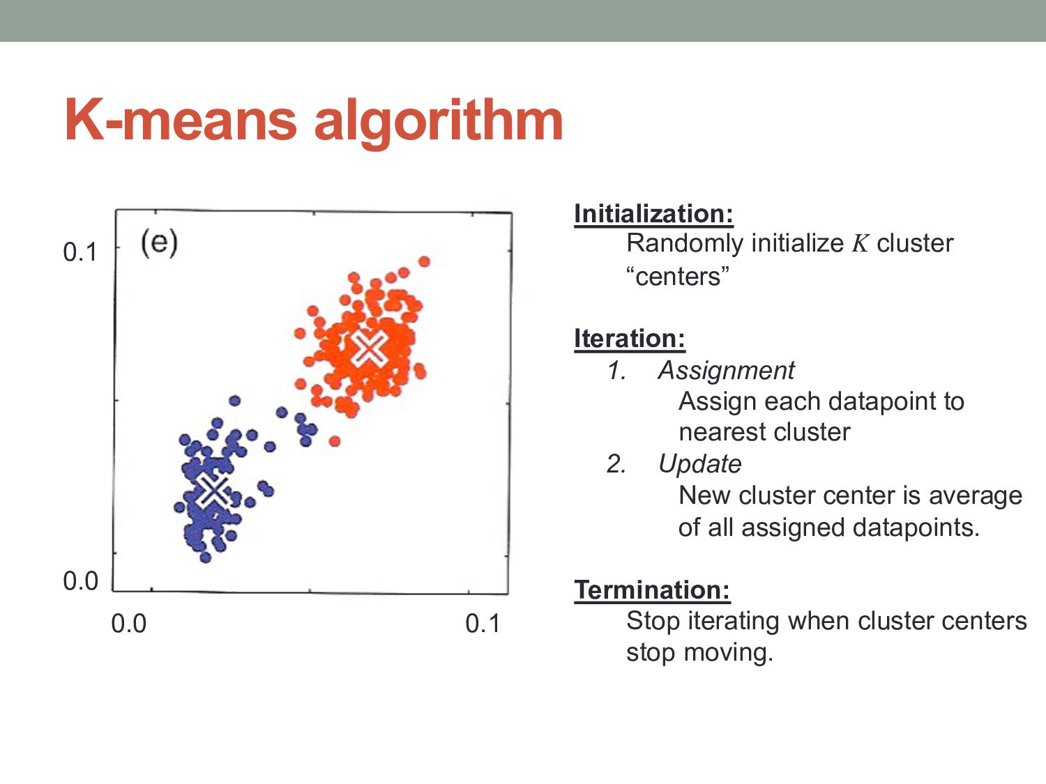
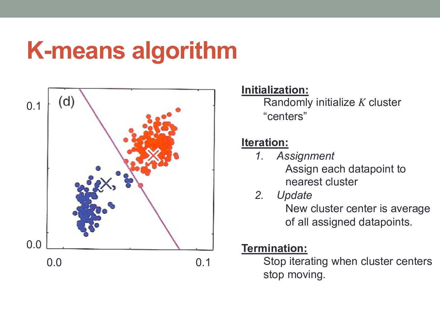
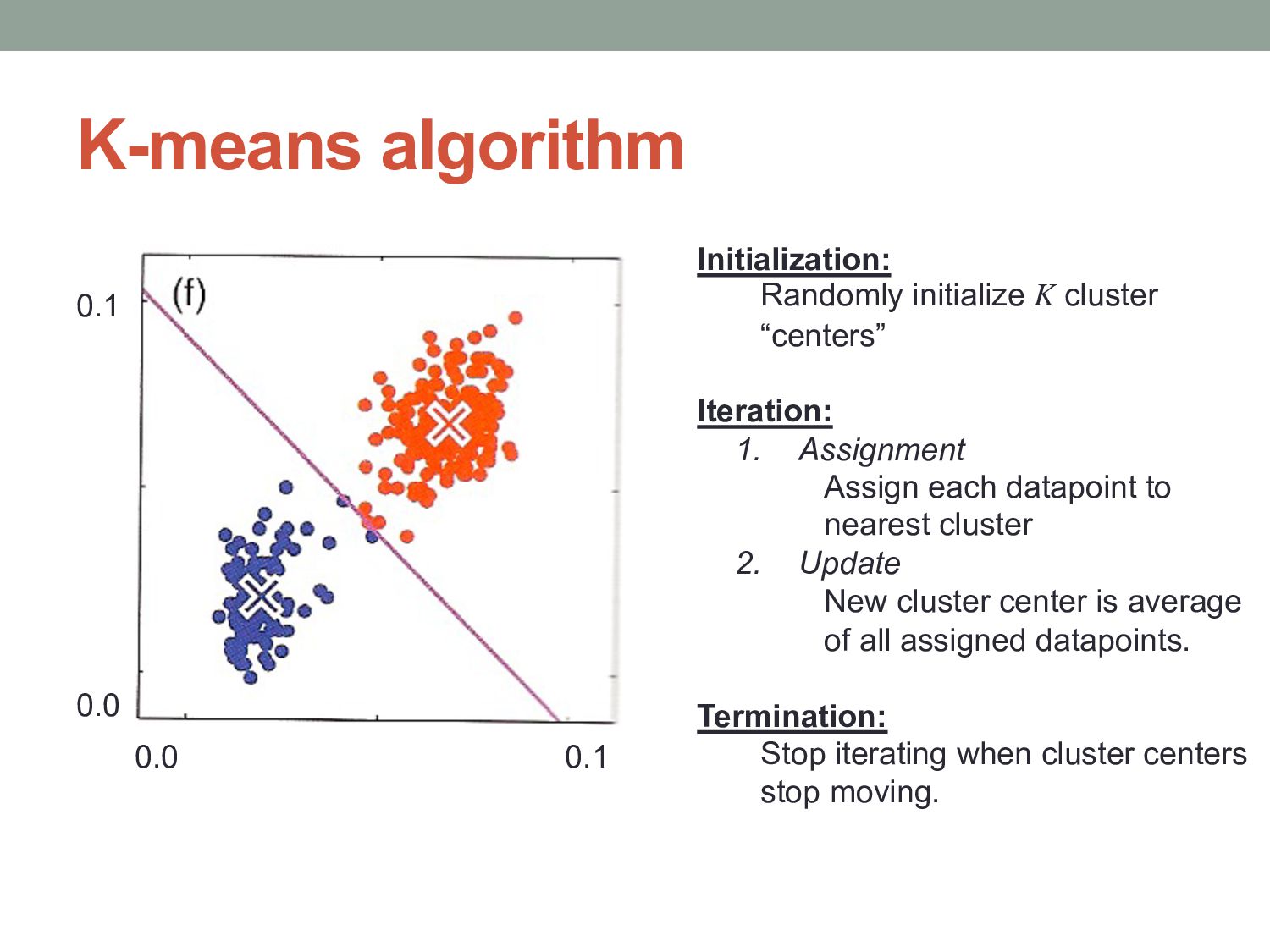
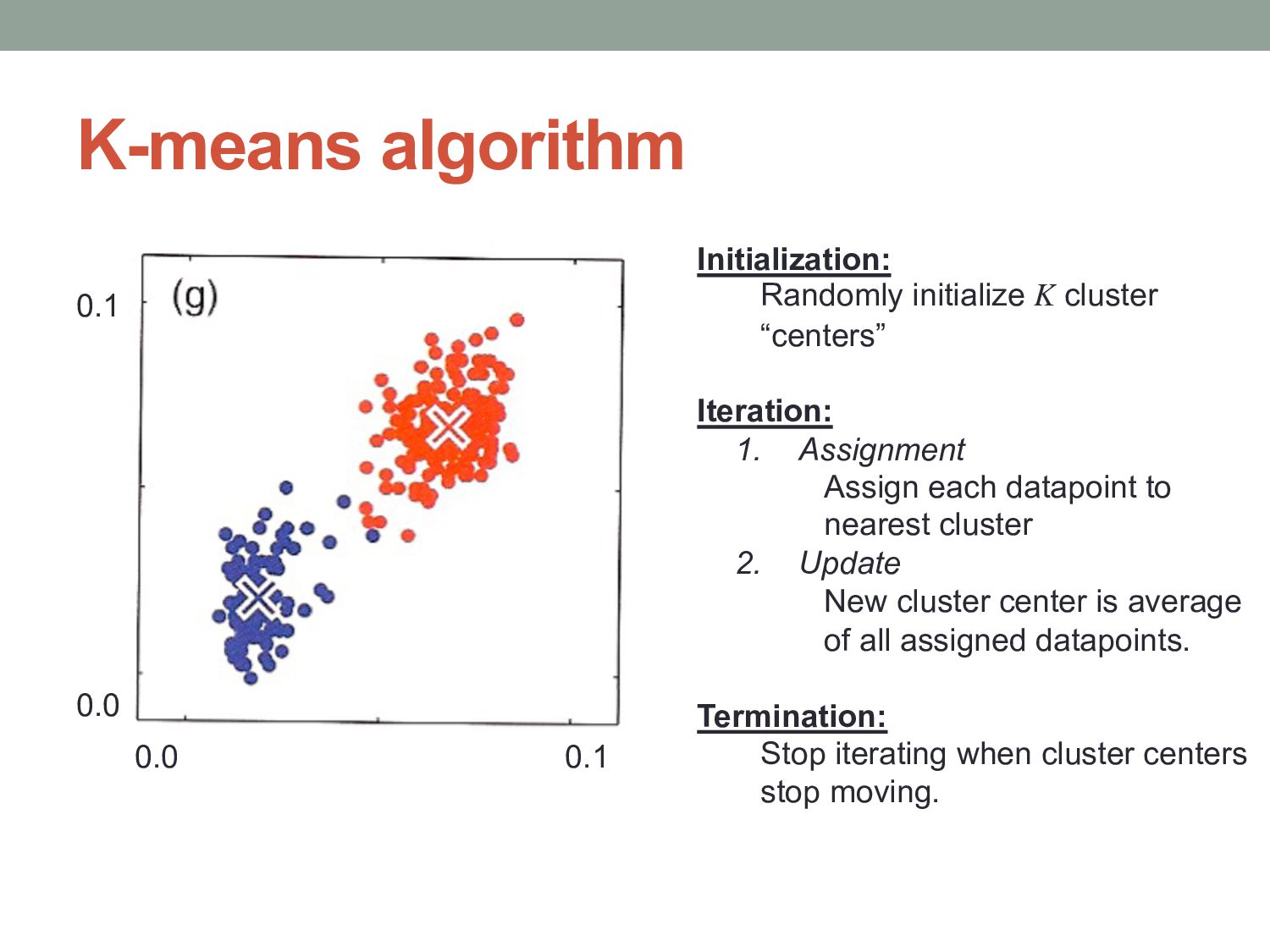
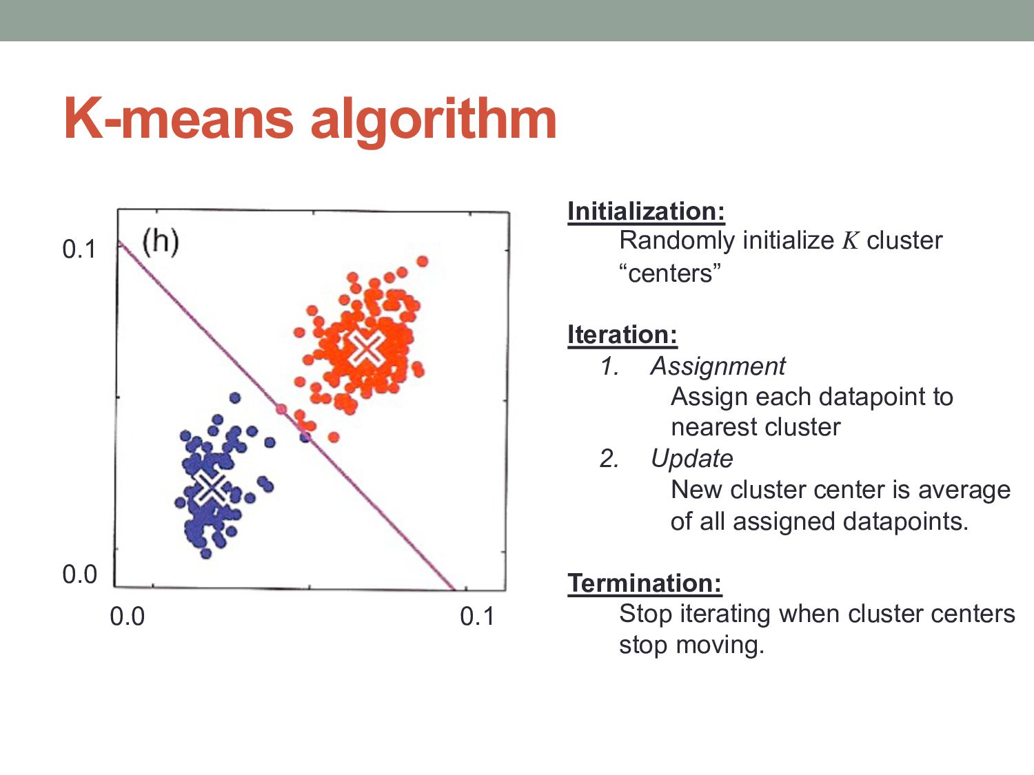
8. K-means algorithm 0.0 0.1 0.1 0.0 Initialization: Randomly initialize K cluster “centers” Iteration: 1. Assignment Assign each datapoint to nearest cluster 2. Update New cluster center is average of all assigned datapoints. Termination: Stop iterating when cluster centers stop moving.
9. K-means algorithm 0.0 0.1 0.1 0.0 Initialization: Randomly initialize K cluster “centers” Iteration: 1. Assignment Assign each datapoint to nearest cluster 2. Update New cluster center is average of all assigned datapoints. Termination: Stop iterating when cluster centers stop moving.
10. K-means algorithm 0.0 0.1 0.1 0.0 Initialization: Randomly initialize K cluster “centers” Iteration: 1. Assignment Assign each datapoint to nearest cluster 2. Update New cluster center is average of all assigned datapoints. Termination: Stop iterating when cluster centers stop moving.
11. K-means algorithm 0.0 0.1 0.1 0.0 Initialization: Randomly initialize K cluster “centers” Iteration: 1. Assignment Assign each datapoint to nearest cluster 2. Update New cluster center is average of all assigned datapoints. Termination: Stop iterating when cluster centers stop moving.
12. K-means Christopher Bishop: “Pattern Recognition and Machine Learning” (Chapter 9)
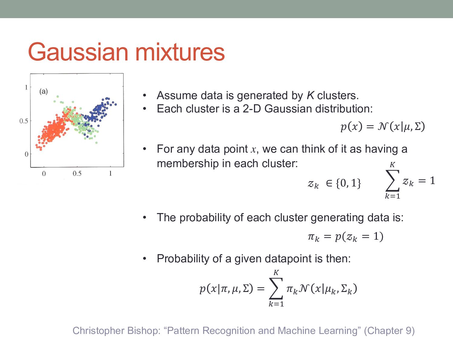
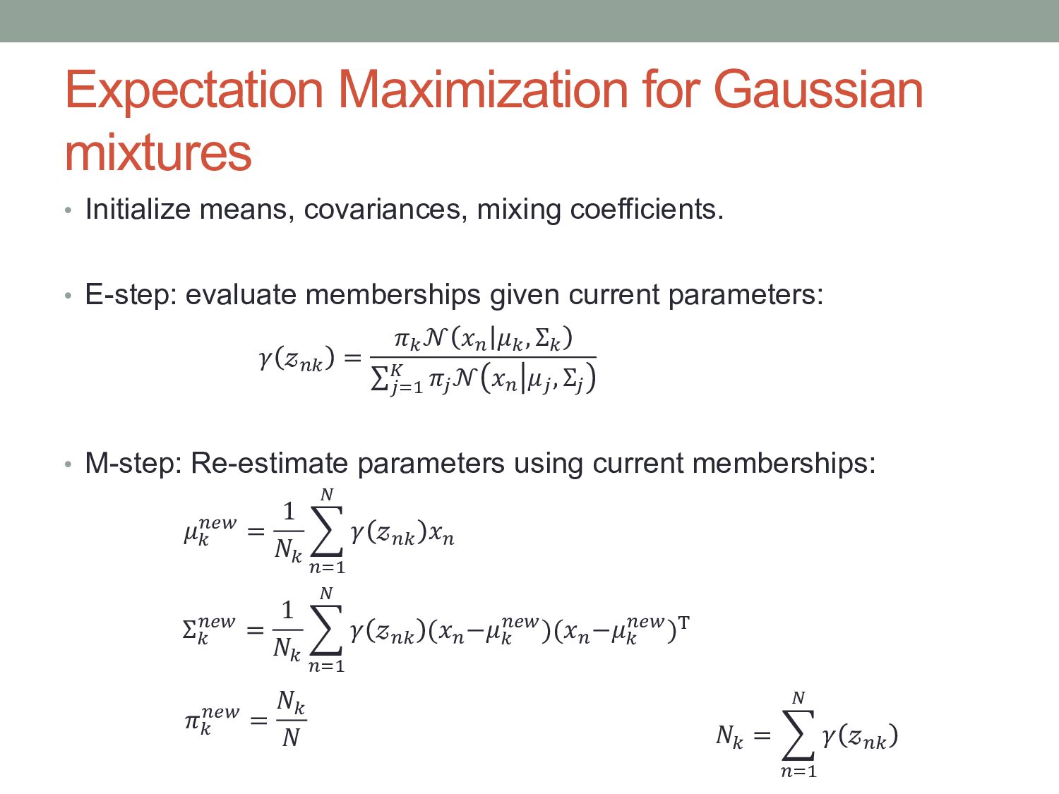
13. Gaussian mixtures Christopher Bishop: “Pattern Recognition and Machine Learning” (Chapter 9) • Assume data is generated by K clusters. • Each cluster is a 2-D Gaussian distribution: • For any data point x, we can think of it as having a membership in each cluster: • The probability of each cluster generating data is: • Probability of a given datapoint is then: 𝑝 𝑥 = 𝒩 𝑥 𝜇, Σ 𝑝 𝑥|𝜋, 𝜇, Σ = * !"# $ 𝜋! 𝒩 𝑥 𝜇! , Σ! 𝜋! = 𝑝(𝓏! = 1) 𝓏! ∈ {0, 1} * !"# $ 𝓏! = 1
14. Gaussian mixtures Christopher Bishop: “Pattern Recognition and Machine Learning” (Chapter 9)
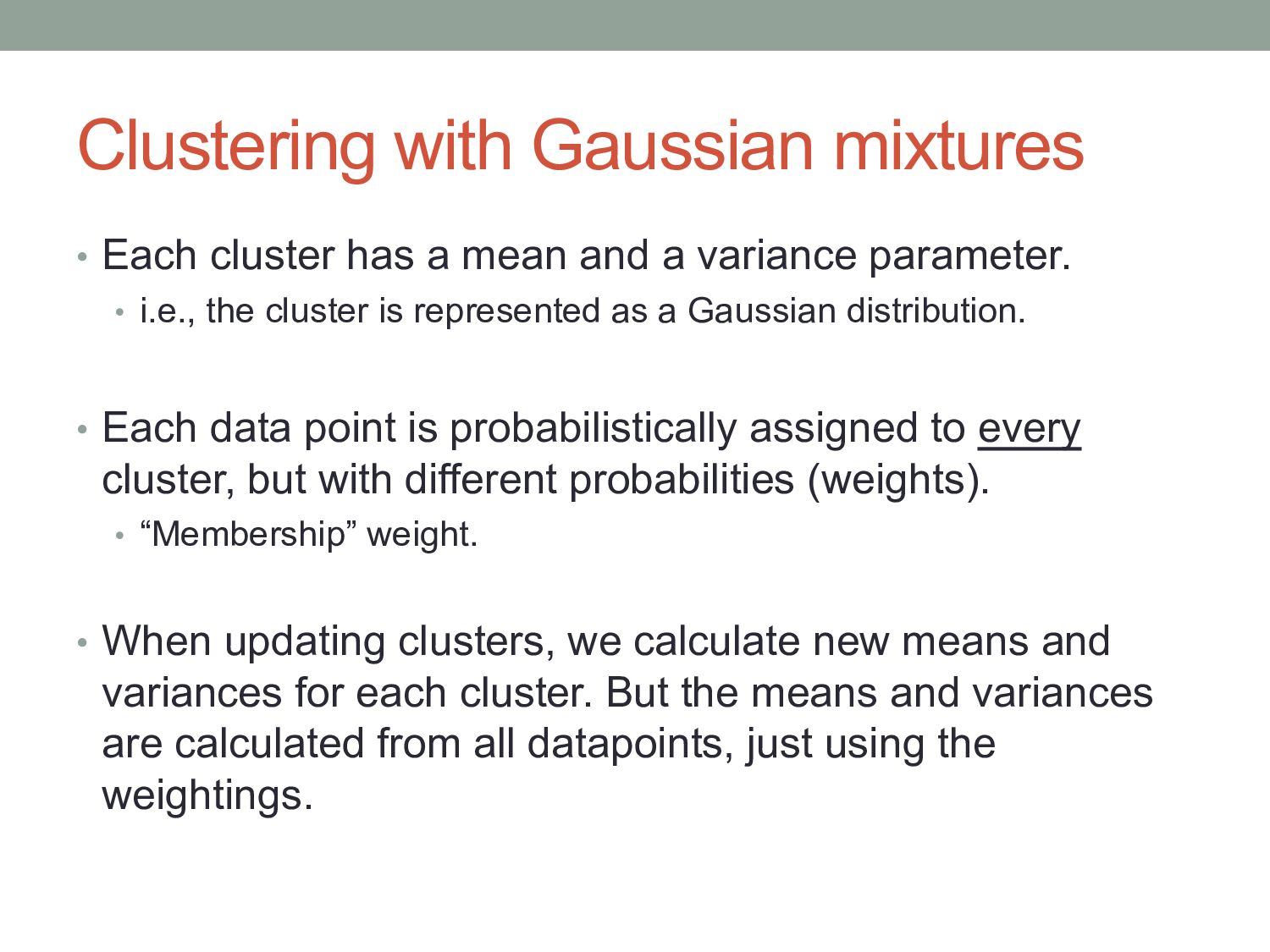
15. Clustering with Gaussian mixtures • Each cluster has a mean and a variance parameter. • i.e., the cluster is represented as a Gaussian distribution. • Each data point is probabilistically assigned to every cluster, but with different probabilities (weights). • “Membership” weight. • When updating clusters, we calculate new means and variances for each cluster. But the means and variances are calculated from all datapoints, just using the weightings.
16. Expectation Maximization for Gaussian mixtures • Initialize means, covariances, mixing coefficients. • E-step: evaluate memberships given current parameters: • M-step: Re-estimate parameters using current memberships: 𝛾 𝓏%! = 𝜋! 𝒩 𝑥% 𝜇! , Σ! ∑ &"# $ 𝜋& 𝒩 𝑥% 𝜇& , Σ& 𝜇! %'( = 1 𝑁! * %"# ) 𝛾 𝓏%! 𝑥% Σ! %'( = 1 𝑁! * %"# ) 𝛾 𝓏%! (𝑥% −𝜇! %'()(𝑥% −𝜇! %'()* 𝜋! %'( = 𝑁! 𝑁 𝑁! = * %"# ) 𝛾 𝓏%!
17. De novo motif-finding problem • GIVEN • A set of unaligned sequences that contain instances of a motif • The expected motif length (k) • The form of the data model • i.e., how do we group data into “motif” and “non-motif”? • An objective function • i.e., a way of quantifying the way that a model fits data • FIND • The motif that optimizes the objective function
18. Discovering regulatory motifs • Problem: We hypothesize that a set of sequences may be bound by the same regulator – can we discover shared patterns? • Methods: Mixture models / Expectation Maximization >YBR018C GAL7 GACGGTAGCAACAAGAATATAGCACGAGCCGCGGAGTTCATTTCGTTACTTTTGATATCACTCACAACTATTGCGAAGCGCTTCAGTGAAAAAATCATAA GGAAAAGTTGTAAATATTATTGGTAGTATTCGTTTGGTAAAGTAGAGGGGGTAATTTTTCCCCTTTATTTTGTTCATACATTCTTAAATTGCTTTGCCTC TCCTTTTGGAAAGCTATACTTCGGAGCACTGTTGAGCGAAGGCTCATTAGATATATTTTCTGTCATTTTCCTTAACCCAAAAATAAGGGAAAGGGTCCAA AAAGCGCTCGGACAACTGTTGACCGTGATCCGAAGGACTGGCTATACAGTGTTCACAAAATAGCCAAGCTGAAAATAATGTGTAGCTATGTTCAGTTAGT TTGGCTAGCAAAGATATAAAAGCAGGTCGGAAATATTTATGGGCATTATTATGCAGAGCATCAACATGATA >YBR019C GAL10 ATCGCTTCGCTGATTAATTACCCCAGAAATAAGGCTAAAAAACTAATCGCATTATCATCCTATGGTTGTTAATTTGATTCGTTAATTTGAAGGTTTGTGG GGCCAGGTTCTGCCAATTTTTCCTCTTCATAACCATAAAAGCTAGTATTGTAGAATCTTTATTGTTCGGAGCAGTGCGGCGCGAGGCACATCTGCGTTTC AGGAACGCGACCGGTGAAGACGAGGACGCACGGAGGAGAGTCTTCCGTCGGAGGGCTGTCGCCCGCTCGGCGGCTTCTAATCCGTACTTCAATATAGCAA TGAGCAGTTAAGCGTATTACTGAAAGTTCCAAAGAGAAGGTTTTTTTAGGCTAAGATAATGGGGCTCTTTACATTTCCACAACATATAAGTAAGATTAGA TATGGATATGTATATGGTGGTAATGCCATGTAATATGATTATTAAACTTCTTTGCGTCCATCCAAAAAAAAAG >YBR020W GAL1 ACATGGCATTACCACCATATACATATCCATATCTAATCTTACTTATATGTTGTGGAAATGTAAAGAGCCCCATTATCTTAGCCTAAAAAAACCTTCTCTT TGGAACTTTCAGTAATACGCTTAACTGCTCATTGCTATATTGAAGTACGGATTAGAAGCCGCCGAGCGGGCGACAGCCCTCCGACGGAAGACTCTCCTCC GTGCGTCCTCGTCTTCACCGGTCGCGTTCCTGAAACGCAGATGTGCCTCGCGCCGCACTGCTCCGAACAATAAAGATTCTACAATACTAGCTTTTATGGT TATGAAGAGGAAAAATTGGCAGTAACCTGGCCCCACAAACCTTCAAATTAACGAATCAAATTAACAACCATAGGATGATAATGCGATTAGTTTTTTAGCC TTATTTCTGGGGTAATTAATCAGCGAAGCGATGATTTTTGATCTATTAACAGATATATAAATGGAAAAGCTGCATAACCACTTTAACTAATACTTTCAAC ATTTTCAGTTTGTATTACTTCTTATTCAAATGTCATAAAAGTATCAACAAAAAATTGTTAATATACCTCTATA >YLR081W GAL2 AGGTTGCAATTTCTTTTTCTATTAGTAGCTAAAAATGGGTCACGTGATCTATATTCGAAAGGGGCGGTTGCCTCAGGAAGGCACCGGCGGTCTTTCGTCC GTGCGGAGATATCTGCGCCGTTCAGGGGTCCATGTGCCTTGGACGATATTAAGGCAGAAGGCAGTATCGGGGCGGATCACTCCGAACCGAGATTAGTTAA GCCCTTCCCATCTCAAGATGGGGAGCAAATGGCATTATACTCCTGCTAGAAAGTTAACTGTGCACATATTCTTAAATTATACAACATTCTGGAGAGCTAT TGTTCAAAAAACAAACATTTCGCAGGCTAAAATGTGGAGATAGGATAAGTTTTGTAGACATATATAAACAATCAGTAATTGGATTGAAAATTTGGTGTTG TGAATTGCTCTTCATTATGCACCTTATTCAATTATCATCAAGAATAGTAATAGTTAAGTAAACACAAGATTA >YBR018C GAL7 GACGGTAGCAACAAGAATATAGCACGAGCCGCGGAGTTCATTTCGTTACTTTTGATATCACTCACAACTATTGCGAAGCGCTTCAGTGAAAAAATCATAA GGAAAAGTTGTAAATATTATTGGTAGTATTCGTTTGGTAAAGTAGAGGGGGTAATTTTTCCCCTTTATTTTGTTCATACATTCTTAAATTGCTTTGCCTC TCCTTTTGGAAAGCTATACTTCGGAGCACTGTTGAGCGAAGGCTCATTAGATATATTTTCTGTCATTTTCCTTAACCCAAAAATAAGGGAAAGGGTCCAA AAAGCGCTCGGACAACTGTTGACCGTGATCCGAAGGACTGGCTATACAGTGTTCACAAAATAGCCAAGCTGAAAATAATGTGTAGCTATGTTCAGTTAGT TTGGCTAGCAAAGATATAAAAGCAGGTCGGAAATATTTATGGGCATTATTATGCAGAGCATCAACATGATA >YBR019C GAL10 ATCGCTTCGCTGATTAATTACCCCAGAAATAAGGCTAAAAAACTAATCGCATTATCATCCTATGGTTGTTAATTTGATTCGTTAATTTGAAGGTTTGTGG GGCCAGGTTCTGCCAATTTTTCCTCTTCATAACCATAAAAGCTAGTATTGTAGAATCTTTATTGTTCGGAGCAGTGCGGCGCGAGGCACATCTGCGTTTC AGGAACGCGACCGGTGAAGACGAGGACGCACGGAGGAGAGTCTTCCGTCGGAGGGCTGTCGCCCGCTCGGCGGCTTCTAATCCGTACTTCAATATAGCAA TGAGCAGTTAAGCGTATTACTGAAAGTTCCAAAGAGAAGGTTTTTTTAGGCTAAGATAATGGGGCTCTTTACATTTCCACAACATATAAGTAAGATTAGA TATGGATATGTATATGGTGGTAATGCCATGTAATATGATTATTAAACTTCTTTGCGTCCATCCAAAAAAAAAG >YBR020W GAL1 ACATGGCATTACCACCATATACATATCCATATCTAATCTTACTTATATGTTGTGGAAATGTAAAGAGCCCCATTATCTTAGCCTAAAAAAACCTTCTCTT TGGAACTTTCAGTAATACGCTTAACTGCTCATTGCTATATTGAAGTACGGATTAGAAGCCGCCGAGCGGGCGACAGCCCTCCGACGGAAGACTCTCCTCC GTGCGTCCTCGTCTTCACCGGTCGCGTTCCTGAAACGCAGATGTGCCTCGCGCCGCACTGCTCCGAACAATAAAGATTCTACAATACTAGCTTTTATGGT TATGAAGAGGAAAAATTGGCAGTAACCTGGCCCCACAAACCTTCAAATTAACGAATCAAATTAACAACCATAGGATGATAATGCGATTAGTTTTTTAGCC TTATTTCTGGGGTAATTAATCAGCGAAGCGATGATTTTTGATCTATTAACAGATATATAAATGGAAAAGCTGCATAACCACTTTAACTAATACTTTCAAC ATTTTCAGTTTGTATTACTTCTTATTCAAATGTCATAAAAGTATCAACAAAAAATTGTTAATATACCTCTATA >YLR081W GAL2 AGGTTGCAATTTCTTTTTCTATTAGTAGCTAAAAATGGGTCACGTGATCTATATTCGAAAGGGGCGGTTGCCTCAGGAAGGCACCGGCGGTCTTTCGTCC GTGCGGAGATATCTGCGCCGTTCAGGGGTCCATGTGCCTTGGACGATATTAAGGCAGAAGGCAGTATCGGGGCGGATCACTCCGAACCGAGATTAGTTAA GCCCTTCCCATCTCAAGATGGGGAGCAAATGGCATTATACTCCTGCTAGAAAGTTAACTGTGCACATATTCTTAAATTATACAACATTCTGGAGAGCTAT TGTTCAAAAAACAAACATTTCGCAGGCTAAAATGTGGAGATAGGATAAGTTTTGTAGACATATATAAACAATCAGTAATTGGATTGAAAATTTGGTGTTG TGAATTGCTCTTCATTATGCACCTTATTCAATTATCATCAAGAATAGTAATAGTTAAGTAAACACAAGATTA
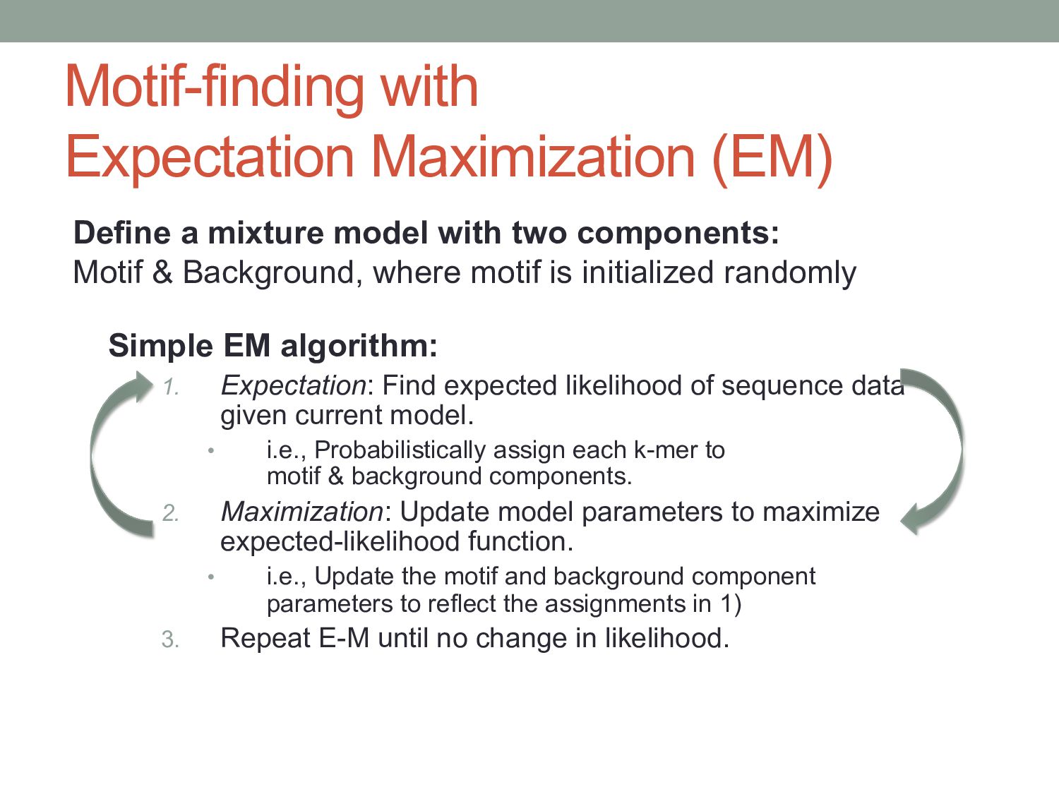
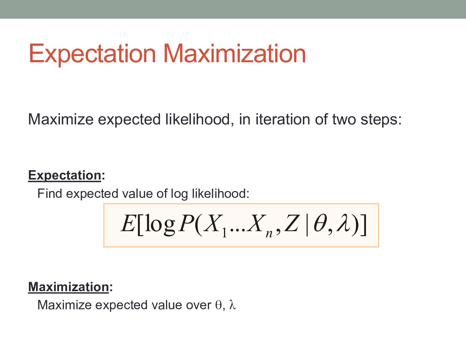
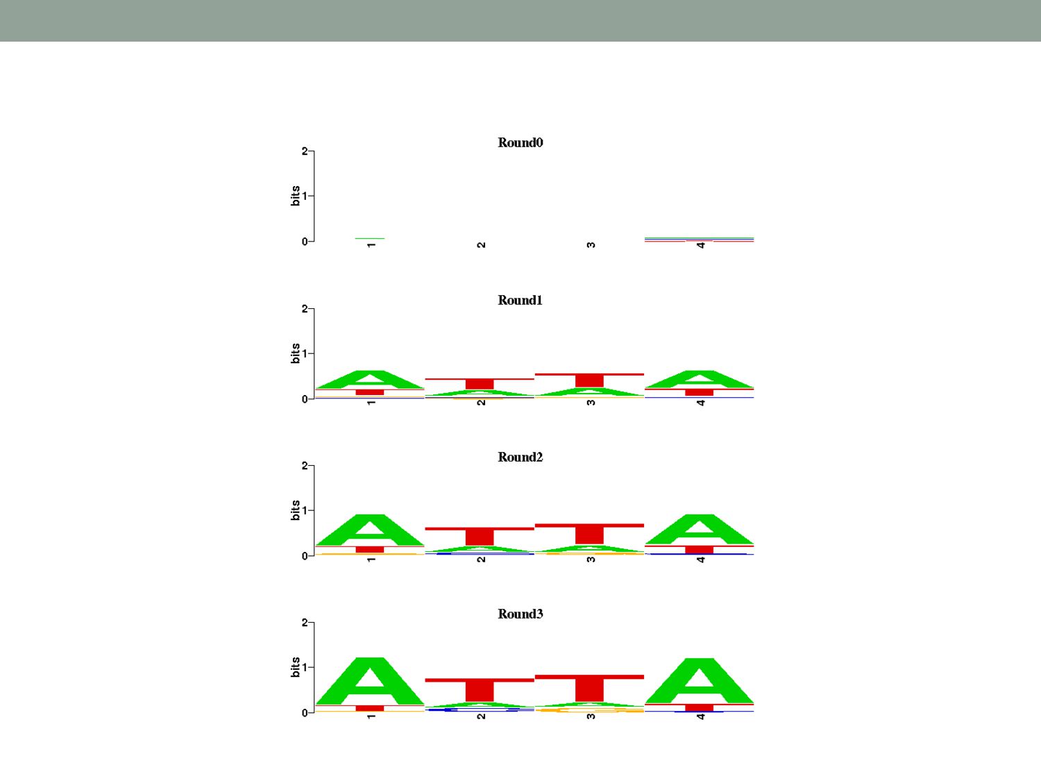
19. Motif-finding with Expectation Maximization (EM) Simple EM algorithm: 1. Expectation: Find expected likelihood of sequence data given current model. • i.e., Probabilistically assign each k-mer to motif & background components. 2. Maximization: Update model parameters to maximize expected-likelihood function. • i.e., Update the motif and background component parameters to reflect the assignments in 1) 3. Repeat E-M until no change in likelihood. Define a mixture model with two components: Motif & Background, where motif is initialized randomly
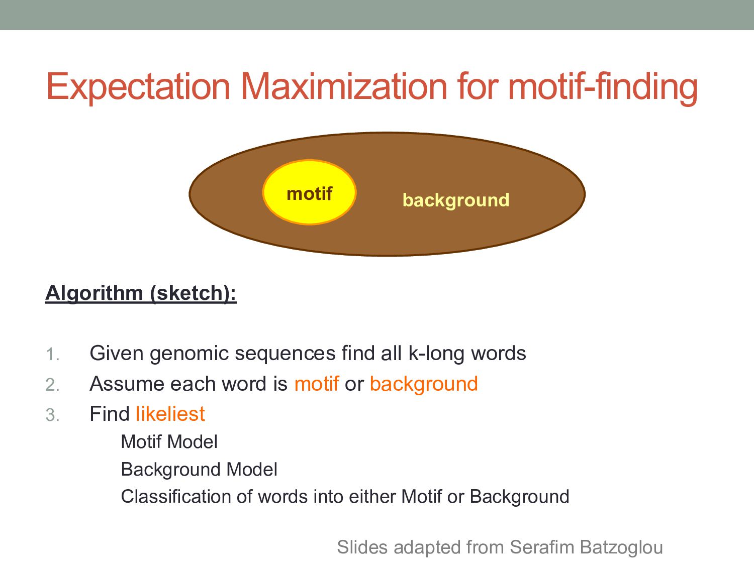
20. All K-long words motif background Expectation Maximization for motif-finding Algorithm (sketch): 1. Given genomic sequences find all k-long words 2. Assume each word is motif or background 3. Find likeliest Motif Model Background Model Classification of words into either Motif or Background Slides adapted from Serafim Batzoglou
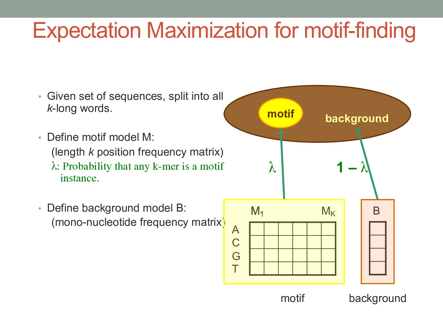
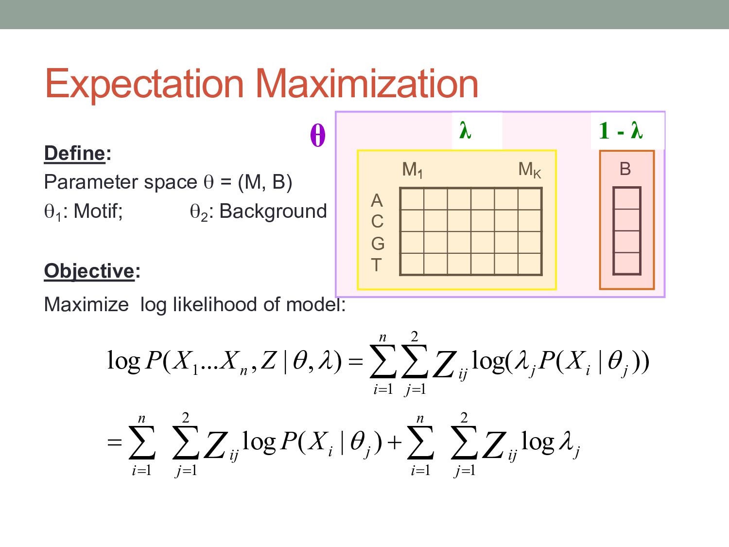
21. Expectation Maximization for motif-finding • Given set of sequences, split into all k-long words. • Define motif model M: (length k position frequency matrix) λ: Probability that any k-mer is a motif instance. • Define background model B: (mono-nucleotide frequency matrix) motif background A C G T M1 MK M1 B motif background λ 1 – λ
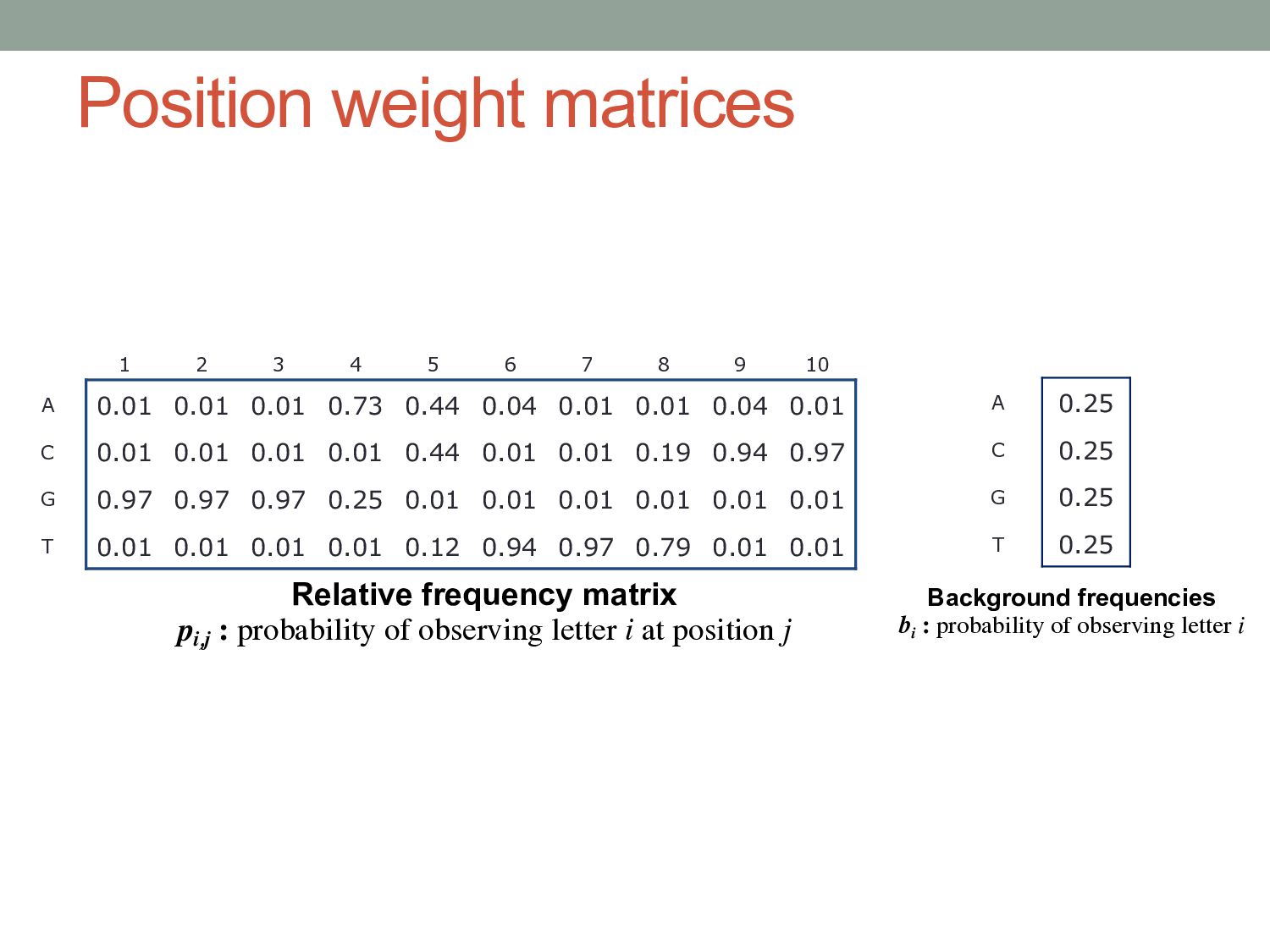
22. Position weight matrices 1 2 3 4 5 6 7 8 9 10 A 0.01 0.01 0.01 0.73 0.44 0.04 0.01 0.01 0.04 0.01 C 0.01 0.01 0.01 0.01 0.44 0.01 0.01 0.19 0.94 0.97 G 0.97 0.97 0.97 0.25 0.01 0.01 0.01 0.01 0.01 0.01 T 0.01 0.01 0.01 0.01 0.12 0.94 0.97 0.79 0.01 0.01 Relative frequency matrix pi,j : probability of observing letter i at position j A 0.25 C 0.25 G 0.25 T 0.25 Background frequencies bi : probability of observing letter i
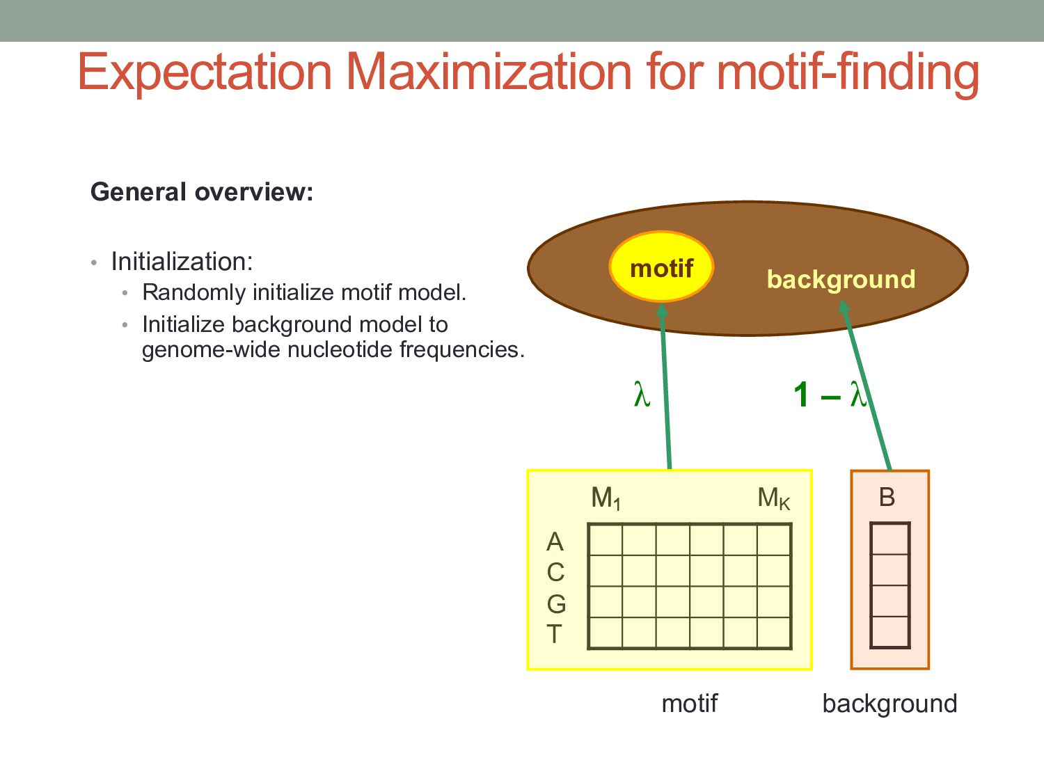
23. Expectation Maximization for motif-finding General overview: • Initialization: • Randomly initialize motif model. • Initialize background model to genome-wide nucleotide frequencies. motif background A C G T M1 MK M1 B motif background λ 1 – λ
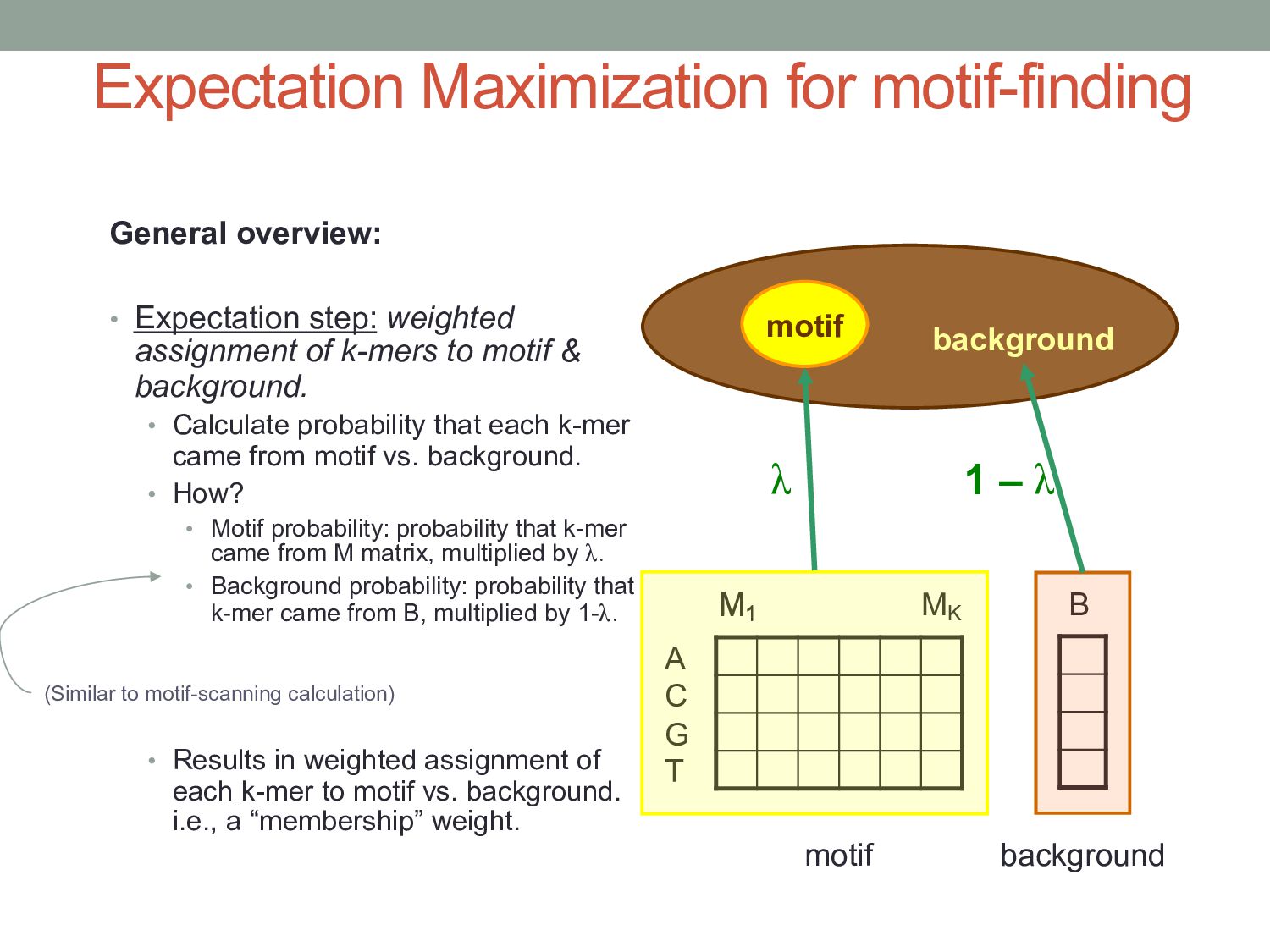
24. Expectation Maximization for motif-finding General overview: • Expectation step: weighted assignment of k-mers to motif & background. • Calculate probability that each k-mer came from motif vs. background. • How? • Motif probability: probability that k-mer came from M matrix, multiplied by λ. • Background probability: probability that k-mer came from B, multiplied by 1-λ. • Results in weighted assignment of each k-mer to motif vs. background. i.e., a “membership” weight. motif background A C G T M1 MK M1 B motif background λ 1 – λ (Similar to motif-scanning calculation)
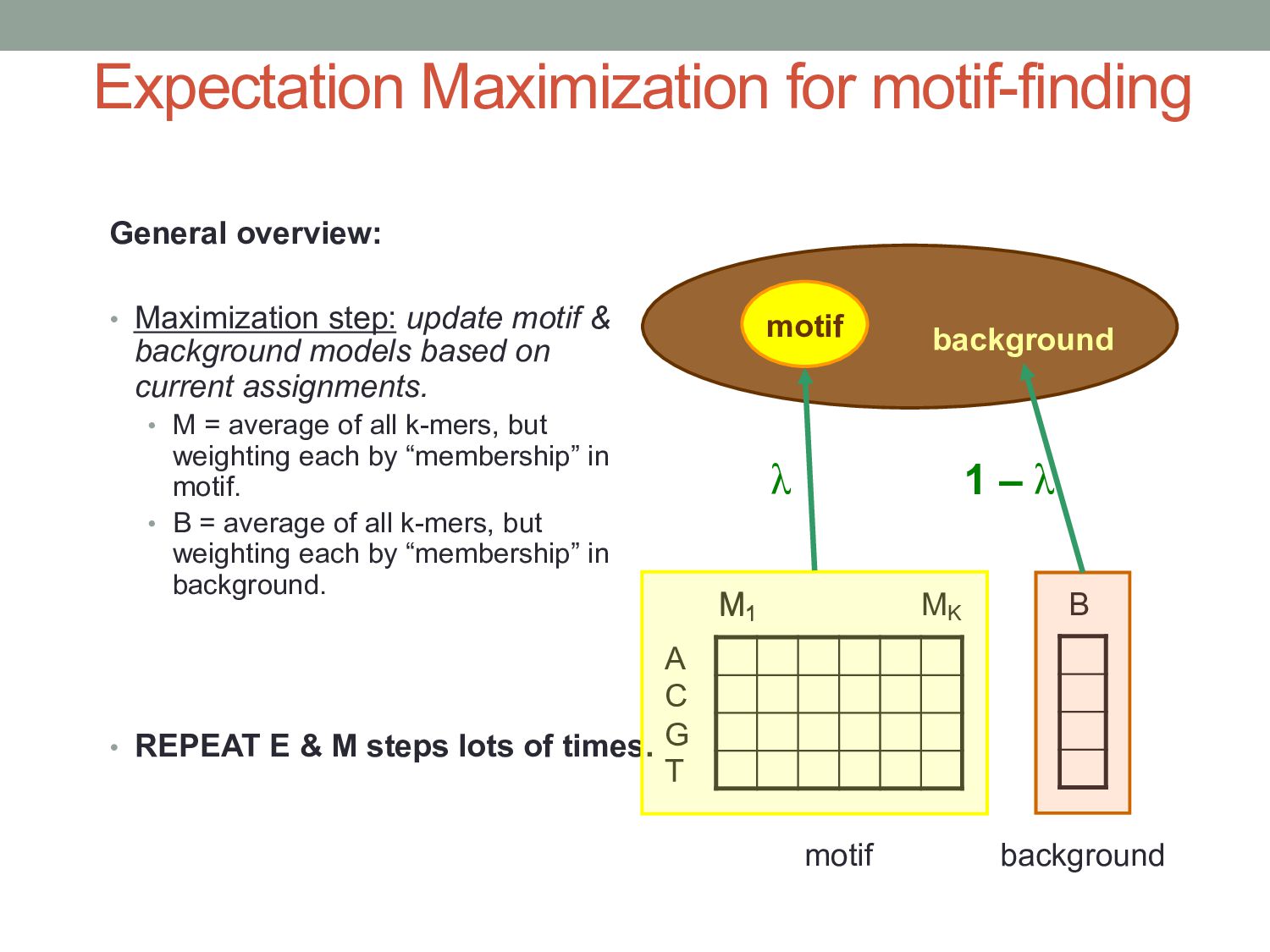
25. Expectation Maximization for motif-finding General overview: • Maximization step: update motif & background models based on current assignments. • M = average of all k-mers, but weighting each by “membership” in motif. • B = average of all k-mers, but weighting each by “membership” in background. • REPEAT E & M steps lots of times. motif background A C G T M1 MK M1 B motif background λ 1 – λ
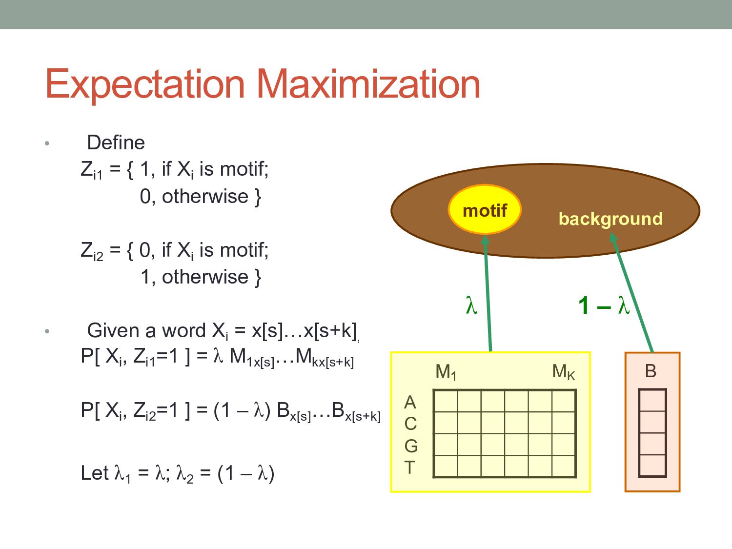
26. Expectation Maximization • Define Zi1 = { 1, if Xi is motif; 0, otherwise } Zi2 = { 0, if Xi is motif; 1, otherwise } • Given a word Xi = x[s]…x[s+k], P[ Xi , Zi1 =1 ] = λ M1x[s] …Mkx[s+k] P[ Xi , Zi2 =1 ] = (1 – λ) Bx[s] …Bx[s+k] Let λ1 = λ; λ2 = (1 – λ) motif background A C G T M1 MK M1 B λ 1 – λ
27. Expectation Maximization Define: Parameter space θ = (M, B) θ1 : Motif; θ2 : Background Objective: Maximize log likelihood of model: å å å å åå = = = = = = + = = 2 1 2 1 1 1 1 2 1 1 log ) | ( log )) | ( log( ) , | , ... ( log j j j ij n i j i ij n i n i j j i j ij n Z Z Z X P X P Z X X P l q q l l q A C G T M1 MK M1 B l 1 – l θ λ 1 - λ
28. Expectation Maximization Maximize expected likelihood, in iteration of two steps: Expectation: Find expected value of log likelihood: Maximization: Maximize expected value over θ, λ )] , | , ... ( [log 1 l q Z X X P E n
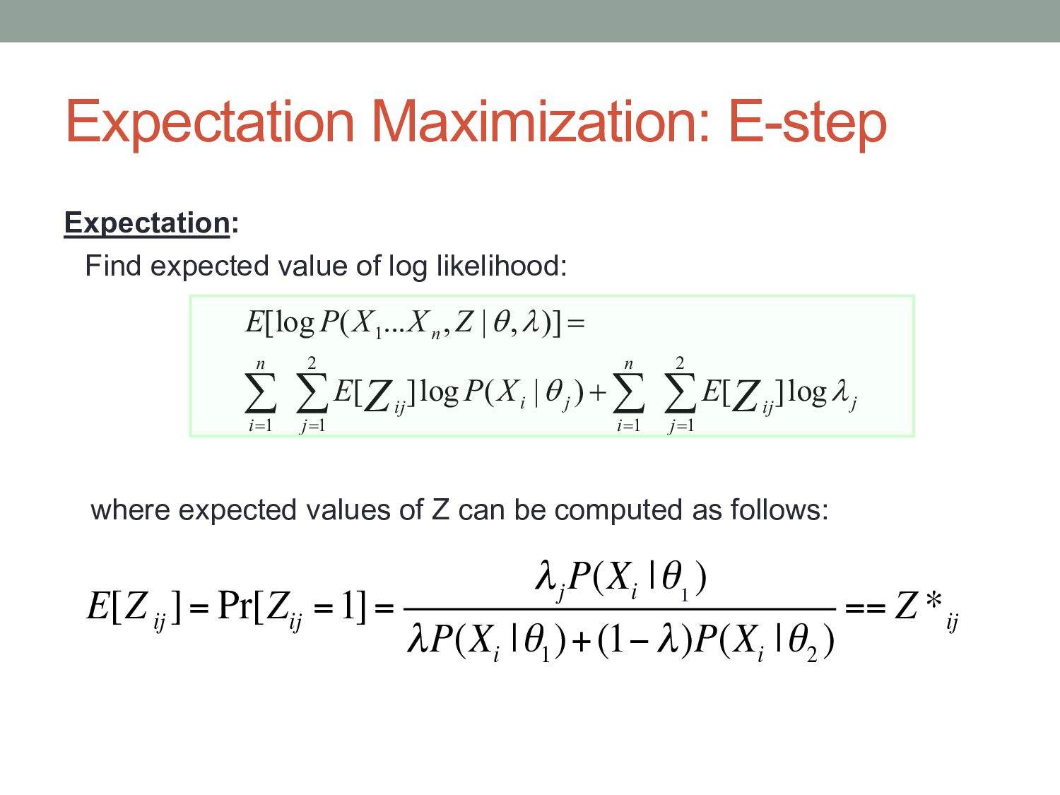
29. Expectation: Find expected value of log likelihood: å å å å = = = = + = 2 1 2 1 1 1 1 log ] [ ) | ( log ] [ )] , | , ... ( [log j j j ij n i j i ij n i n Z Z E X P E Z X X P E l q l q !"#$#%#&'#()#*%+,-.#/%01%2%(,3%4#%(05'.)#*%,/%10--0!/6 E[Z ij ]= Pr[Z ij =1]= λj P(X i |θj ) λP(X i |θ1 )+(1−λ)P(X i |θ2 ) == Z * ij Expectation Maximization: E-step 1
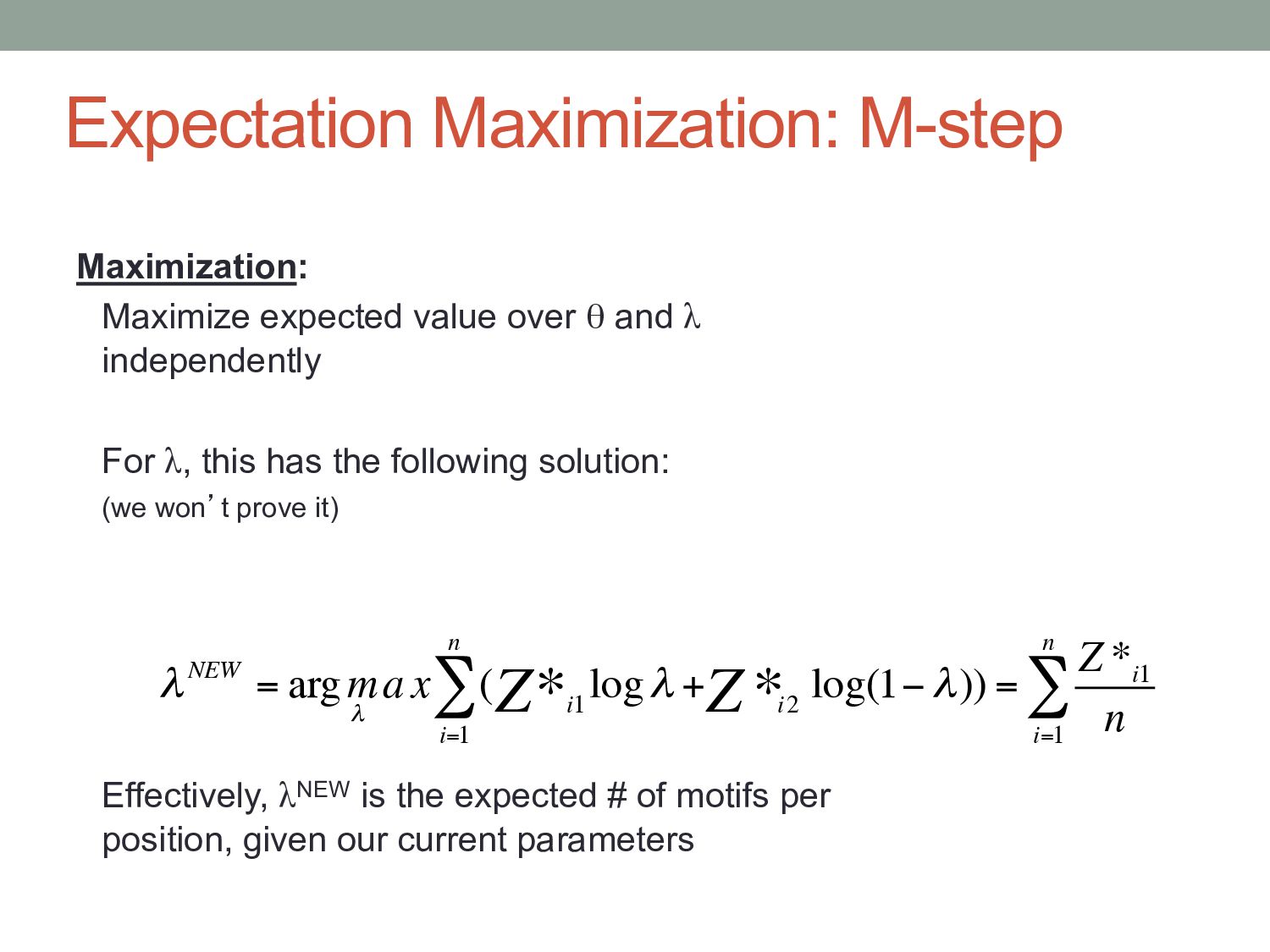
30. Expectation Maximization: M-step Maximization: Maximize expected value over θ and λ independently For λ, this has the following solution: (we won’t prove it) Effectively, λNEW is the expected # of motifs per position, given our current parameters λNEW = argm λ a x ( i1 Z* logλ + i2 Z * log(1− λ)) = Z * i1 n i=1 n ∑ i=1 n ∑
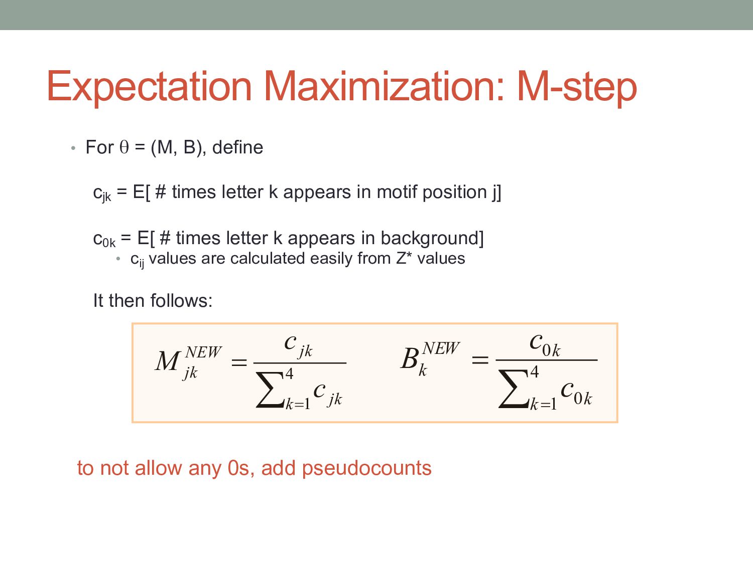
31. • For θ = (M, B), define cjk = E[ # times letter k appears in motif position j] c0k = E[ # times letter k appears in background] • cij values are calculated easily from Z* values It then follows: å = = 4 1 k jk jk NEW jk c c M å = = 4 1 0 0 k k k NEW k c c B )0%30)%,--0!%,37%8/9%,**%'/#.*0(0.3)/ Expectation Maximization: M-step
32. Motif-finding example • Find a length 4 motif in the following sequence: ATTACGATTAAATTA • Random starting motif: • Uniform background (A=C=G=T=0.25) • λmotif = 0.2, λbackground = 0.8 Motif 1 2 3 4 A 0.4 0.25 0.25 0.35 C 0.2 0.2 0.25 0.3 G 0.2 0.25 0.2 0.1 T 0.2 0.3 0.3 0.25
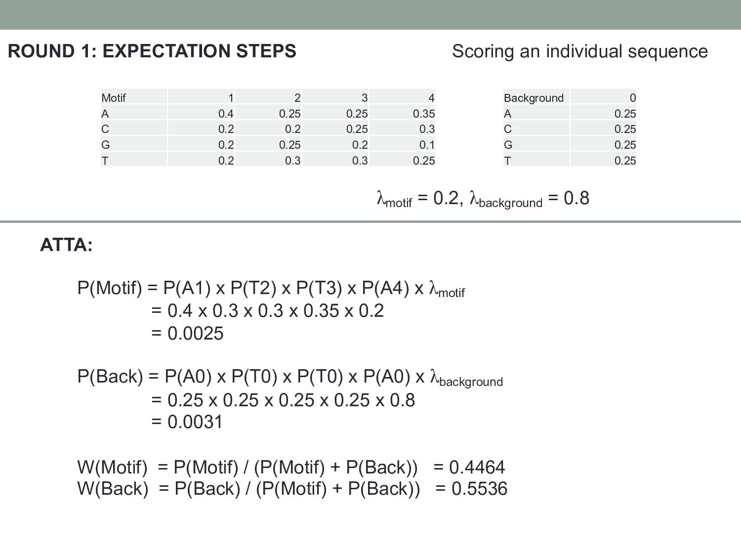
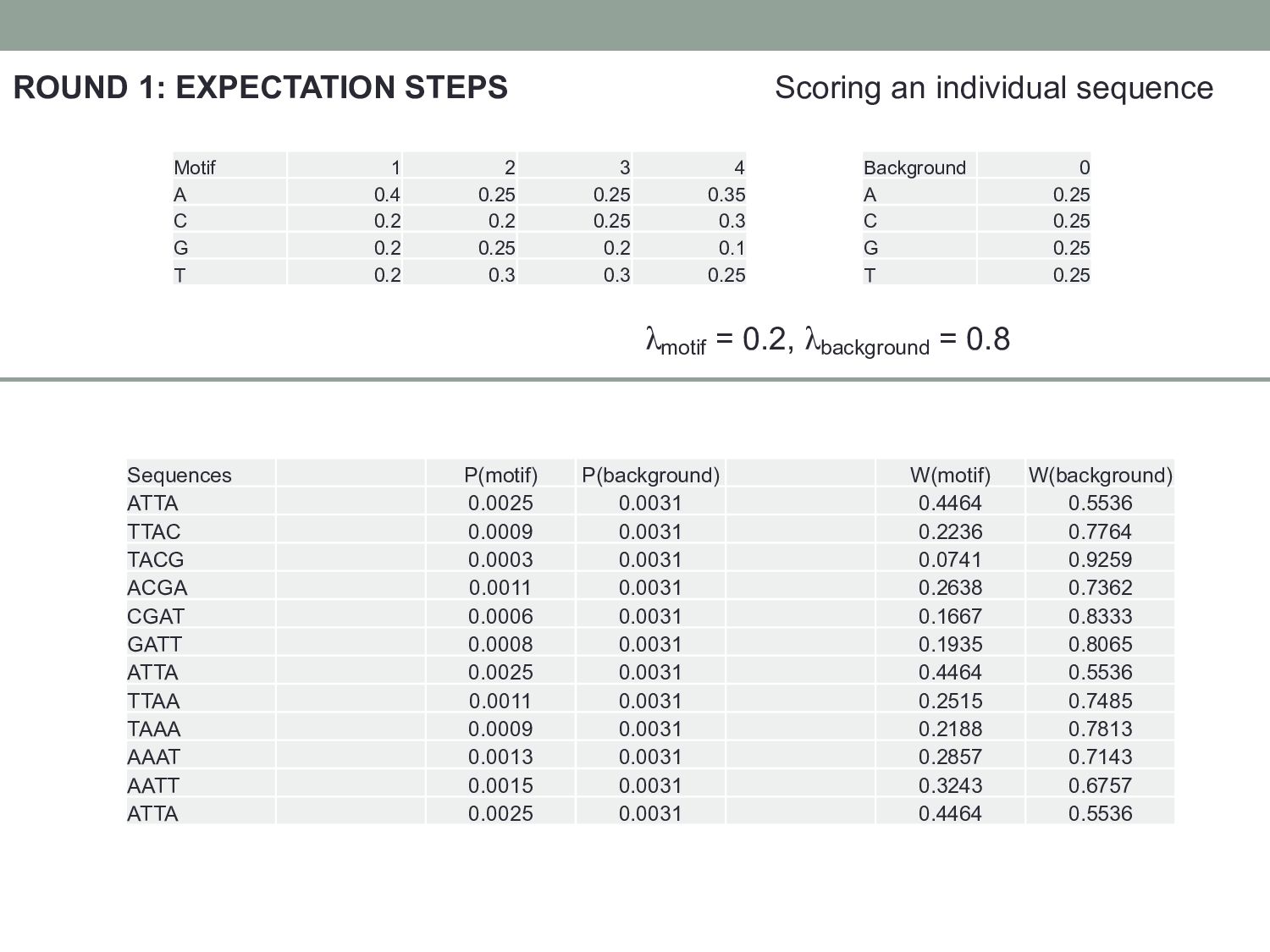
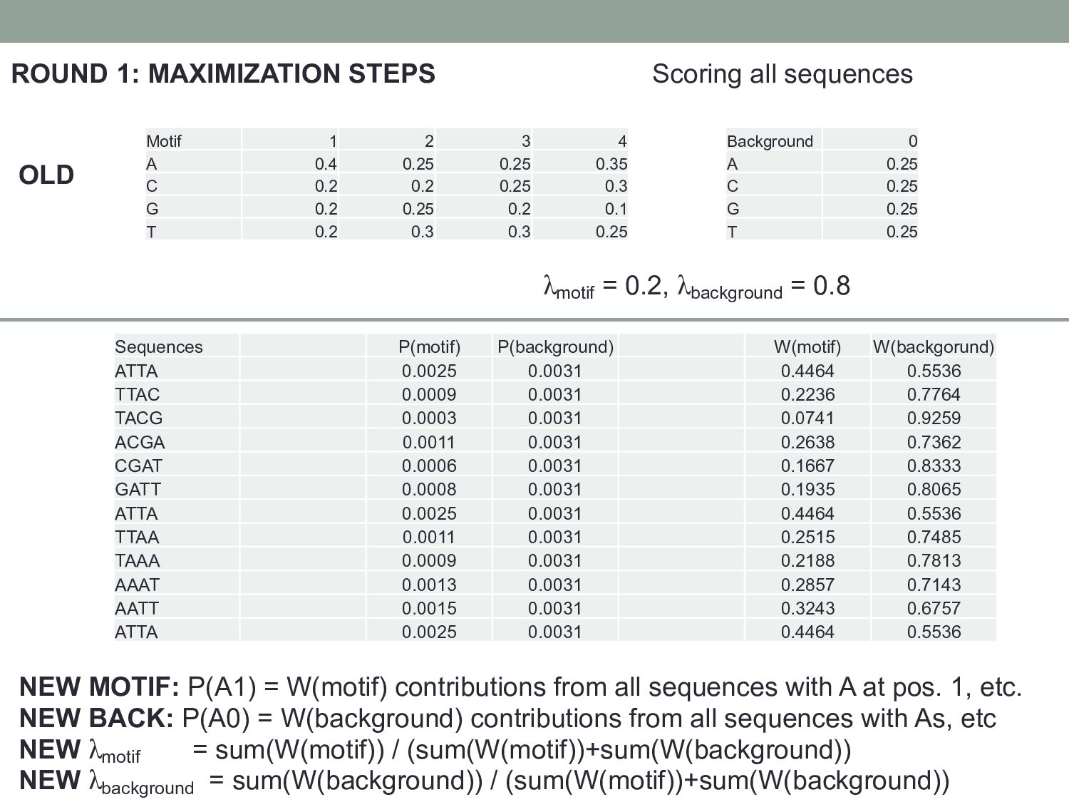
33. ROUND 1: EXPECTATION STEPS Scoring an individual sequence Motif 1 2 3 4 Background 0 A 0.4 0.25 0.25 0.35 A 0.25 C 0.2 0.2 0.25 0.3 C 0.25 G 0.2 0.25 0.2 0.1 G 0.25 T 0.2 0.3 0.3 0.25 T 0.25 ATTA: P(Motif) = P(A1) x P(T2) x P(T3) x P(A4) x λmotif = 0.4 x 0.3 x 0.3 x 0.35 x 0.2 = 0.0025 P(Back) = P(A0) x P(T0) x P(T0) x P(A0) x λbackground = 0.25 x 0.25 x 0.25 x 0.25 x 0.8 = 0.0031 W(Motif) = P(Motif) / (P(Motif) + P(Back)) = 0.4464 W(Back) = P(Back) / (P(Motif) + P(Back)) = 0.5536 λmotif = 0.2, λbackground = 0.8
34. ROUND 1: EXPECTATION STEPS Scoring an individual sequence Motif 1 2 3 4 Background 0 A 0.4 0.25 0.25 0.35 A 0.25 C 0.2 0.2 0.25 0.3 C 0.25 G 0.2 0.25 0.2 0.1 G 0.25 T 0.2 0.3 0.3 0.25 T 0.25 λmotif = 0.2, λbackground = 0.8 Sequences P(motif) P(background) W(motif) W(background) ATTA 0.0025 0.0031 0.4464 0.5536 TTAC 0.0009 0.0031 0.2236 0.7764 TACG 0.0003 0.0031 0.0741 0.9259 ACGA 0.0011 0.0031 0.2638 0.7362 CGAT 0.0006 0.0031 0.1667 0.8333 GATT 0.0008 0.0031 0.1935 0.8065 ATTA 0.0025 0.0031 0.4464 0.5536 TTAA 0.0011 0.0031 0.2515 0.7485 TAAA 0.0009 0.0031 0.2188 0.7813 AAAT 0.0013 0.0031 0.2857 0.7143 AATT 0.0015 0.0031 0.3243 0.6757 ATTA 0.0025 0.0031 0.4464 0.5536
35. ROUND 1: MAXIMIZATION STEPS Scoring all sequences Motif 1 2 3 4 Background 0 A 0.4 0.25 0.25 0.35 A 0.25 C 0.2 0.2 0.25 0.3 C 0.25 G 0.2 0.25 0.2 0.1 G 0.25 T 0.2 0.3 0.3 0.25 T 0.25 λmotif = 0.2, λbackground = 0.8 Sequences P(motif) P(background) W(motif) W(backgorund) ATTA 0.0025 0.0031 0.4464 0.5536 TTAC 0.0009 0.0031 0.2236 0.7764 TACG 0.0003 0.0031 0.0741 0.9259 ACGA 0.0011 0.0031 0.2638 0.7362 CGAT 0.0006 0.0031 0.1667 0.8333 GATT 0.0008 0.0031 0.1935 0.8065 ATTA 0.0025 0.0031 0.4464 0.5536 TTAA 0.0011 0.0031 0.2515 0.7485 TAAA 0.0009 0.0031 0.2188 0.7813 AAAT 0.0013 0.0031 0.2857 0.7143 AATT 0.0015 0.0031 0.3243 0.6757 ATTA 0.0025 0.0031 0.4464 0.5536 OLD NEW MOTIF: P(A1) = W(motif) contributions from all sequences with A at pos. 1, etc. NEW BACK: P(A0) = W(background) contributions from all sequences with As, etc NEW λmotif = sum(W(motif)) / (sum(W(motif))+sum(W(background)) NEW λbackground = sum(W(background)) / (sum(W(motif))+sum(W(background))
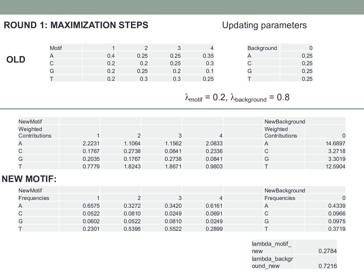
36. ROUND 1: MAXIMIZATION STEPS Updating parameters Motif 1 2 3 4 Background 0 A 0.4 0.25 0.25 0.35 A 0.25 C 0.2 0.2 0.25 0.3 C 0.25 G 0.2 0.25 0.2 0.1 G 0.25 T 0.2 0.3 0.3 0.25 T 0.25 λmotif = 0.2, λbackground = 0.8 OLD NewMotif NewBackground Weighted Contributions 1 2 3 4 Weighted Contributions 0 A 2.2231 1.1064 1.1562 2.0833 A 14.6897 C 0.1767 0.2738 0.0841 0.2336 C 3.2718 G 0.2035 0.1767 0.2738 0.0841 G 3.3019 T 0.7779 1.8243 1.8671 0.9803 T 12.5904 NewMotif NewBackground Frequencies 1 2 3 4 Frequencies 0 A 0.6575 0.3272 0.3420 0.6161 A 0.4339 C 0.0522 0.0810 0.0249 0.0691 C 0.0966 G 0.0602 0.0522 0.0810 0.0249 G 0.0975 T 0.2301 0.5395 0.5522 0.2899 T 0.3719 lambda_motif_ new 0.2784 lambda_backgr ound_new 0.7216 NEW MOTIF:
37. ROUND 2: EXPECTATION STEPS λmotif = 0.2784, λbackground = 0.7216 Motif 1 2 3 4 Background 0 A 0.6575 0.3272 0.3420 0.6161 A 0.4339 C 0.0522 0.0810 0.0249 0.0691 C 0.0966 G 0.0602 0.0522 0.0810 0.0249 G 0.0975 T 0.2301 0.5395 0.5522 0.2899 T 0.3719 Sequences P(motif) P(background) W(motif) W(backgorund) ATTA 0.0336 0.0188 0.6414 0.3586 TTAC 0.0008 0.0042 0.1632 0.8368 TACG 0.0000 0.0011 0.0117 0.9883 ACGA 0.0007 0.0013 0.3662 0.6338 CGAT 0.0001 0.0011 0.0642 0.9358 GATT 0.0009 0.0042 0.1721 0.8279 ATTA 0.0336 0.0188 0.6414 0.3586 TTAA 0.0073 0.0188 0.2793 0.7207 TAAA 0.0044 0.0219 0.1677 0.8323 AAAT 0.0059 0.0219 0.2131 0.7869 AATT 0.0096 0.0188 0.3379 0.6621 ATTA 0.0336 0.0188 0.6414 0.3586
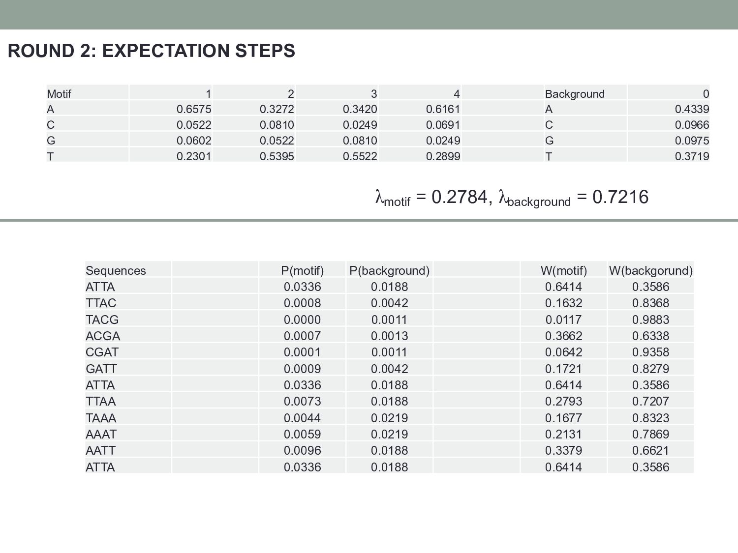
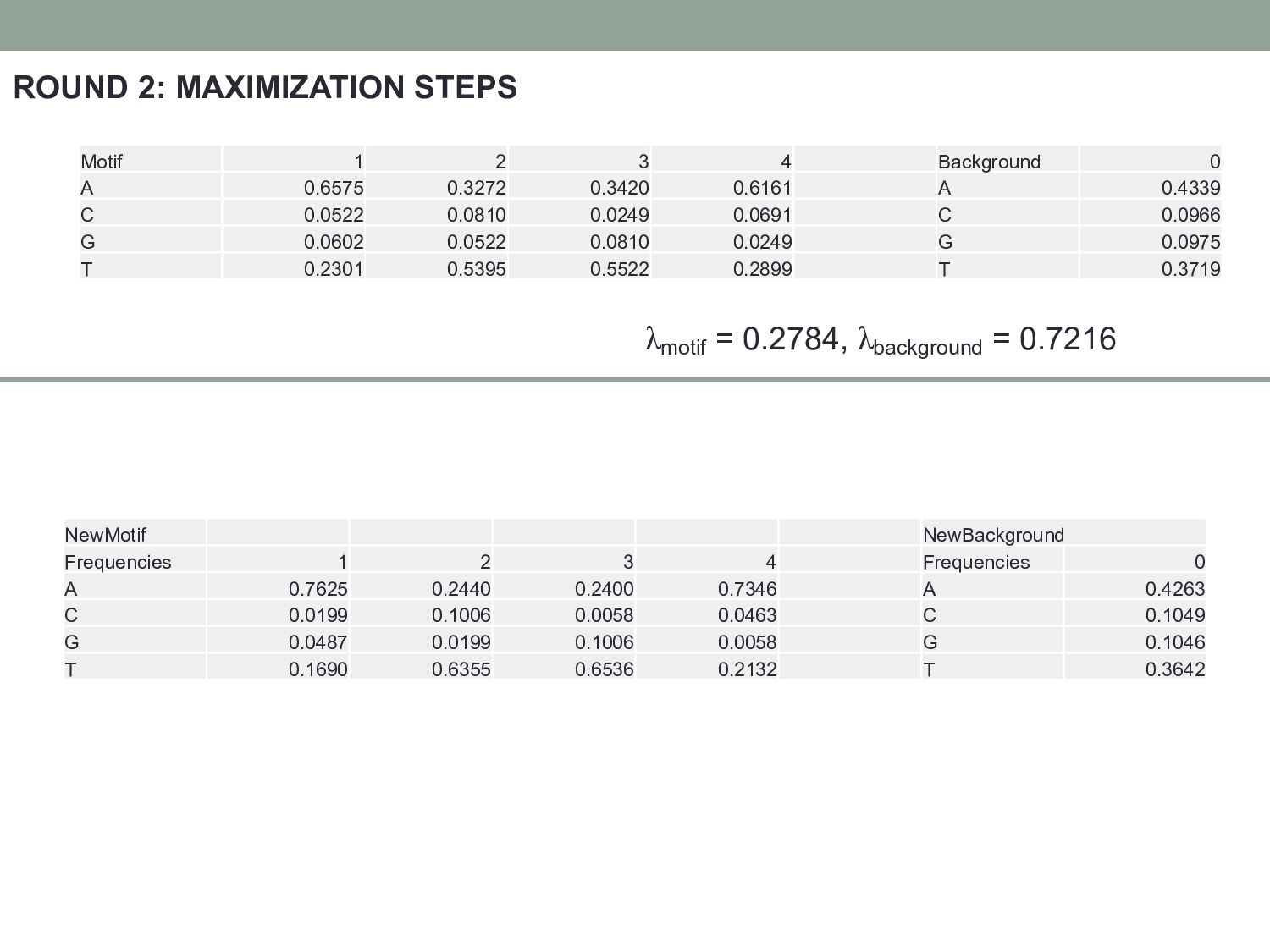
38. ROUND 2: MAXIMIZATION STEPS λmotif = 0.2784, λbackground = 0.7216 Motif 1 2 3 4 Background 0 A 0.6575 0.3272 0.3420 0.6161 A 0.4339 C 0.0522 0.0810 0.0249 0.0691 C 0.0966 G 0.0602 0.0522 0.0810 0.0249 G 0.0975 T 0.2301 0.5395 0.5522 0.2899 T 0.3719 NewMotif NewBackground Frequencies 1 2 3 4 Frequencies 0 A 0.7625 0.2440 0.2400 0.7346 A 0.4263 C 0.0199 0.1006 0.0058 0.0463 C 0.1049 G 0.0487 0.0199 0.1006 0.0058 G 0.1046 T 0.1690 0.6355 0.6536 0.2132 T 0.3642
40. Problems… • EM not guaranteed to find the globally optimal motif. • How do we know the length of the motif? • EM approach assumes one motif in the data… what if there are more? • Is the model too simplistic?
41. Further reading • Motif scanning & motif-finding: • “Practical strategies for discovering regulatory DNA sequence motifs”, MacIsaac & Fraenkel, PLoS Comp Bio (2006) • “Applied bioinformatics for the identification of regulatory elements”, Wasserman & Sandelin, Nature Rev Genetics (2004) • MEME: • “Fitting a mixture model by expectation maximization to discover motifs in biopolymers”, Bailey & Elkan, Proc. ISMB (1994) • Gene regulation & Gal4 system: “Genes & Signals”, Ptashne & Gann (2002)
42. Summary • Motif-finding approaches can be used to discover over- represented sequence patterns in collections of sequences. • Expectation Maximization (EM) is a machine-learning approach that iteratively estimates/optimizes parameters in a statistical model. • EM can be used to discover motif signals in statistical models that include TF binding motifs vs. unbound sequence.
44. FINDING TF BINDING EVENTS IN CHIP-SEQ DATA
45. Identifying precise TF binding locations • ChIP-seq reads are distributed bimodally around binding sites. • Regions of ChIP-enrichment are known as “peaks”. Valouev, et al. Nature Methods (2008)
46. Identifying precise TF binding locations
47. Computational challenge: resolve the structure of TF binding events from ChIP-seq data How many binding events are here? How close to the actual bound bases are event predictions? + -
48. Mixture models of ChIP-seq binding events Lhx3 ChIP-seq
49. Mixture models of ChIP-seq binding events Lhx3 ChIP-seq
50. Mixture models of ChIP-seq binding events Lhx3 ChIP-seq
51. Mixture models of ChIP-seq binding events Lhx3 ChIP-seq Predicted binding events: Motif instances: 140bp 160bp
52. GPS/GEM/ChExMix allow more accurate spatial resolution of binding events GEM: http://groups.csail.mit.edu/cgs/gem/
53. Further reading • Park PJ “ChIP-seq: advantages and disadvantages of a maturing technology”, Nature Reviews Genetics (2009) 10(10):669-680 • Landt S, et al. “ChIP-seq guidelines and practices of the ENCODE and modENCODE consortia”, Genome Research (2012) 22:1813 – 1831 • Carroll TS, et al. “Impact of artifact removal on ChIP quality metrics in ChIP-seq and ChIP-exo data”, Frontiers in Genetics (2014) 5:75 • Mahony S & Pugh BF “Protein-DNA binding in high resolution”, Critical Reviews in Biochemistry and Molecular Biology (2015) 4:269-283