A Map of the PyData Stack

A talk given at Toulouse Data Science meetup in April 2016. Slightly adjusted version (I went into more detail due to time) of my talk from PyData Amsterdam. I spoke about the current PyData ecosystem, what you use things for and what you don't. What tools are expected soon and what is mature right now/ will be more mature in the future. Tools mentioned include Dask, Pandas, NumPy, Numba, Cython, Spark and Bcolz. I included code examples too.

Transcript

1. A Map of the Stack
   A Map of the Stack
   

   View Slide

2. Hi I'm Peadar Coyle
   Hi I'm Peadar Coyle
   (Pronounced PAH-DER - I'm Irish)!!
   @springcoil
   @springcoil
   https://github.com/springcoil
   All views are my own and do not represent
   any future, current or past employers.
   Code: http://bit.ly/pydatakeynotespringcoil​
   

   View Slide

3. Who I've worked with
   Who I've worked with
   Contributor to PyMC3 and other open source software
   Author and Speaker at PyData and EuroSciPy
   Check out 'Interviews with Data Scientists' - 24 data
   scientists interviewed - proceeds go to NumFOCUS
   http://bit.ly/interviewswithdatasci​
   

   View Slide

4. My new Adventure
   My new Adventure
   I joined Channel 4 in early April as a Senior Data Scientist to
   work on customer segmentation and recommendation engines
   Channel 4 is an award winning not-for-profit TV channel and
   digital channel. Famous for Father Ted, the IT Crowd and many
   other shows.
   

   View Slide

5. Version 3 is the way forward!
   

   View Slide

6. It's April 2016 I want to do
   It's April 2016 I want to do
   Analytics in PyData
   Analytics in PyData
   It depends what you want to do
   This talk includes sample code
   What is new, what is not new, etc
   Very influenced by
   I'll talk a bit more about Statistics and ML
   There'll be no bikes in my talk :)
   Rob Story
   

   View Slide

7. Why use Python for
   Why use Python for
   Analytics anyway?
   Analytics anyway?
   Although Python is not very fast for things like
   webservers (Go would be better) it is **very** fast
   for things like HPC or Numerics.
   Because of C and Fortran (and maybe others like Rust
   or Theano in the future)
   (HT: Rob Story)
   

   View Slide

8. PyData strengths
   PyData strengths
   A rich and varied ecosystem
   Lots of activities, lots of different ways of attacking
   the same problems
   A great history of attacking hard problems by
   community effort
   

   View Slide

9. And many others.
   Open Source can't thrive without industrial
   and academic support
   Thanks to these guys and girls...
   

   View Slide

10. The PyData Stack
    The PyData Stack
    And many many more...
    

    View Slide

11. Our wonderful ecosystem
    Our wonderful ecosystem
    I'll talk about what is new in PyData
    I'll talk about what tools to use with different
    localities of datasets (in memory, out-of-core and
    distributed)
    I'll talk about our Statistical tools including PyMC3
    I'll talk about the future!!
    

    View Slide

12. What's new and
    What's new and
    useful in PyData
    useful in PyData
    

    View Slide

13. New in the core of
    New in the core of
    the stack
    the stack
    It is impossible to talk about PyData
    It is impossible to talk about PyData
    without mentioning NumPy and
    without mentioning NumPy and
    Pandas
    Pandas
    

    View Slide

14. Improvements throughout the stack
    Matplotlib colours, Sympy new release,
    improvements in NumPy
    New @ operator in NumPy
    Assign, and pipe in Pandas
    

    View Slide

15. Pandas - assign
    Pandas - assign
    df = pd.DataFrame({'A': range(1, 11), 'B': np.random.randn(10)})
    df.assign(ln_A_plus_1=lambda x: np.log(x.A)+1)
    Creates a copy of the dataframe with a
    nice new column.
    Really useful for percentages, logarithms
    etc - standard Financial Analysis and Data
    Analysis stuff.
    

    View Slide

16. View Slide

17. I have a data
    I have a data
    problem to solve
    problem to solve
    In practice grouping and counting
    In practice grouping and counting
    things :)
    things :)
    

    View Slide

18. Adult data set
    data
    age workclass fnlwgt education-categorical educ
    0 39 State-gov 77516 Bachelors 13
    2 38 Private 215646 HS-grad 9
    3 53 Private 234721 11th 7
    4 28 Private 338409 Bachelors 13
    5 37 Private 284582 Masters 14
    6 49 Private 160187 9th 5
    Source UCI Adult data set, csv version
    here: http://pymc-
    devs.github.io/pymc3/Bayesian_LogReg/
    

    View Slide

19. I can only use
    I can only use
    standard library
    standard library
    I'm stuck on a restricted machine and I only have Python
    2.6
    (Example shamelessly stolen from Rob Story and
    adapted for my data set)
    

    View Slide

20. import csv
    conversion_map = {
    'age': int,
    'workclass': str,
    'fnlwgt': int,
    'education-categorical': str,
    'educ': int,
    'occupation': str,
    'sex': str,
    'capital-gain': float,
    'capital-loss': float,
    'hours': int,
    'native-country': str,
    'income': str
    }
    Write a conversion map and use csv
    

    View Slide

21. Load the csv data source
    def converter(type_map, row):
    """Yep, we need to roll our own type conversions."""
    converted_row = {}
    for col, val in row.items():
    converter = type_map.get(col)
    if converter:
    converted_row[col] = converter(val)
    else:
    converted_row[col] = val
    return converted_row
    with open('adult.csv', 'r') as f:
    reader = csv.DictReader(f)
    adult2 = [converter(conversion_map, r) for r in reader]
    

    View Slide

22. How does it look
    >>> adult2[:2]
    [{'': '0',
    'age': 39,
    'capital-loss': 0.0,
    'captial-gain': '2174',
    'educ': 13,
    'education-categorical': ' Bachelors',
    'fnlwgt': 77516,
    'hours': 40,
    'income': ' <=50K',
    'marital-status': ' Never-married',
    'native-country': ' United-States',
    'occupation': ' Adm-clerical',
    'relationship': ' Not-in-family',
    'sex': ' Male',
    'workclass': ' State-gov'},
    

    View Slide

23. I want to get the maximum age in my dataset
    def get_max_age():
    max_age = 0
    for row in adult2:
    if row['age'] > 1 and row['age'] > max_age:
    max_age = row['age']
    return max_age
    >>> get_max_age()
    90
    # Or you could do it like this generator expression
    >>> max(row['age'] for row in adult2 if row['age'] > 1)
    90
    

    View Slide

24. Let's say you wanted to group things
    # defaultdict is awesome. defaultdict is awesome.
    from collections import defaultdict
    def grouper(grouping_col, seq):
    """People have definitely written a faster version than what I'm ab
    Thanks to Rob Story for this one"""
    groups = defaultdict(lambda: defaultdict(list))
    for row in seq:
    group = groups[row[grouping_col]]
    for k, v in row.items():
    if k != grouping_col:
    group[k].append(v)
    return groups
    >>> groups = grouper('occupation', adult2)
    

    View Slide

25. A natural question is the mean number of hours by occupation
    summary = {}
    for group, values in groups.items():
    summary[group] = sum(values['hours']) / len(values['hours'])
    >>> summary
    {' ?': 31.90613130765057,
    ' Adm-clerical': 37.55835543766578,
    ' Armed-Forces': 40.666666666666664,
    ' Craft-repair': 42.30422054159551,
    ' Exec-managerial': 44.9877029021151,
    ' Farming-fishing': 46.989939637826964,
    ' Handlers-cleaners': 37.947445255474456,
    ' Machine-op-inspct': 40.755744255744254,
    ' Other-service': 34.70166919575114,
    ' Priv-house-serv': 32.88590604026846,
    ' Prof-specialty': 42.38671497584541,
    ' Protective-serv': 42.87057010785824,
    ' Sales': 40.78109589041096,
    ' Tech-support': 39.432112068965516,
    ' Transport-moving': 44.65623043206011}
    

    View Slide

26. Interlude: Itertools
    Interlude: Itertools
    It is common advice but it's worth being
    aware of itertools if you want to write
    something like this.
    http://jmduke.com/posts/a-gentle-
    introduction-to-itertools/
    

    View Slide

27. I wanna count things
    I wanna count things
    - in a functional way
    - in a functional way
    

    View Slide

28. PyToolz
    PyToolz
    PSA: PyToolz is awesome allows you to use functional
    programming techniques in Python.
    I want to make it faster - I'll use CyToolz
    http://toolz.readthedocs.org/en/latest/index.html
    

    View Slide

29. PyToolz example
    PyToolz example
    #I wanna see the frequencies of ages in the dataset
    >>> tz.frequencies([r['age'] for r in adult2])
    # Toolz has currying!
    #I want to count by all of the occupations with greater than 15 years of education
    import toolz.curried as tzc
    >>> tzc.pipe(adult2,
    tzc.filter(lambda r: r['educ'] > 15),
    tzc.map(lambda r: (r['occupation'],)),
    tzc.countby(lambda r: r[0]),
    dict)
    {' ?': 15,
    ' Adm-clerical': 5,
    ' Craft-repair': 2,
    ' Exec-managerial': 55,
    ' Farming-fishing': 1,
    ' Machine-op-inspct': 1,
    ' Other-service': 1,
    ' Prof-specialty': 321,
    ' Sales': 8,
    ' Tech-support': 3,
    ' Transport-moving': 1}
    

    View Slide

30. Summary: Toolz
    Summary: Toolz
    Toolz has some great virtues
    Composability: They interoperate due to core data
    structures
    Purity: They don't change their input or rely on external
    state
    Lazy: Only evaluated when needed
    They also support serializability so they're easy to
    accelerate or parallelize
    

    View Slide

31. Interlude
    Interlude
    

    View Slide

32. Pandas
    Pandas
    Not going to talk too much about Pandas in this talk.
    It is fast becoming a stable and core member of the
    PyData stack
    Really useful for indexed data like time series data or csv
    file data
    Statsmodels and seaborn already consider it a core
    member of the stack
    

    View Slide

33. # One little example of the power of the Pandas API
    adult.groupby('educ').mean()
    >>> age fnlwgt captial-gain
    educ
    1 42.764706 235889.372549 898.392157
    2 46.142857 239303.000000 125.875000
    3 42.885886 232448.333333 176.021021
    4 48.445820 188079.171827 233.939628
    5 41.060311 202485.066148 342.089494
    

    View Slide

34. I won't talk about Numpy either
    Xarray and Dask are all either dependent on it or
    strongly influenced by it
    Pandas depends on it
    Many other projects like Scipy depend on it
    The speed optimizations and the ability to release the
    GIL allow this to be very fast for modern hardware
    Recent improvements include the '@' operator
    making it a lot easier to write good linear algebra
    code in NumPy
    

    View Slide

35. End of Interlude
    End of Interlude
    

    View Slide

36. Labelled heterogenous data
    NumPy arrays plus labels - excellent for
    'Scientific data' :) Or multi-indexed data
    I have weather forecasting data in NetCDF
    - this is what you use
    

    View Slide

37. Xarray looks like this
    Xarray looks like this
    arr = np.array([[1, 2, 3, 4],
    [10, 20, 30, 40],
    [100, 200, 300, 400]])
    dim0_coords = ['a', 'b', 'c']
    dim1_coords = ['foo', 'bar', 'baz', 'qux']
    da = xray.DataArray(arr, [('x', dim0_coords), ('y', dim1_coords)])
    da
    da.loc['b']
    There are plenty of examples in the notebooks
    Code: http://bit.ly/pydatakeynotespringcoil​
    

    View Slide

38. >> da[0:3]
    
    array([[ 1, 2, 3, 4],
    [ 10, 20, 30, 40],
    [100, 200, 300, 400]])
    Coordinates:
    * x (x) * y (y) >>> da.dims
    ('x', 'y')
    >> da.coords
    Coordinates:
    * x (x) * y (y) # Get a mean by label
    >> da.mean(dim='y')
    
    array([ 2.5, 25. , 250. ])
    Coordinates:
    * x (x)

    View Slide

39. I want to disconnect or 'decouple' my expressions for
    computations from my backend
    Why can't I do Pandas like things on Postgresql?
    I have some data in CSV, some in HDF5 (PyTables),
    some in my SQL database
    I still run into in-memory problems
    

    View Slide

40. I have bigger-than-I-can-RAM-data
    Getting a bigger machine is overkill
    Why are my analytical expressions tied to my data
    structure?
    Can I have expressions that work across data
    structure *and* storage?
    

    View Slide

41. Blaze: An interface to query data on different
    storage systems
    Dask: Parallel computing through task
    scheduling and blocked algorithms
    Datashape: A data description language
    DyND: A C++ library for dynamic,
    multidimensional arrays
    Odo: Data migration between different
    storage systems
    Blaze Ecosystem
    Blaze Ecosystem
    

    View Slide

42. We'll talk about Dask later
    We'll talk about Dask later
    We'll use Odo and Blaze in this demo
    Datashape and DyND are awesome but I won't talk
    about them
    

    View Slide

43. import blaze as bz
    bz_adult = bz.symbol('adult2', bz.discover(adult))
    >>> type(bz_adult)
    blaze.expr.expressions.Symbol
    >>> mean_age = bz.by(bz_adult.occupation,
    price=bz_adult.age.mean())
    >>> hours_count = bz.by(bz_adult[bz_adult.hours > 35].educ,
    count=bz_adult.workclass.count())
    # We haven't actually computed anything yet!
    # Let's make Pandas compute it.
    bz.compute(mean_age, adult)
    

    View Slide

44. # We have here the count of number of years of education
    # by a certain filter of greater than 35 hours of work per week.
    >>> bz.compute(hours_count, adult)
    educ count
    0 1 51
    1 2 168
    2 3 333
    3 4 646
    4 5 514
    5 6 933
    6 7 1175
    7 8 433
    

    View Slide

45. Let's compute in
    Let's compute in
    Postgres!
    Postgres!
    # Blaze/Odo make it easy to move data between containers
    # Note that we have an empty table already created
    pg_datasource = bz.odo(adult,
    "postgresql://peadarcoyle@localhost/pydata::adult2")
    # Now we're going to use Postgres as our computation engine
    result = bz.compute(hours_count, pg_datasource)
    result
    
    # I don't want a selectable. I want a DataFrame
    # odo again
    bz.odo(bz.compute(hours_count, pg_datasource), pd.DataFrame)
    educ count
    0 8 433
    1 16 413
    2 15 576
    3 4 646
    4 1 51
    

    View Slide

46. Let's store in Bcolz (we'll see Bcolz and
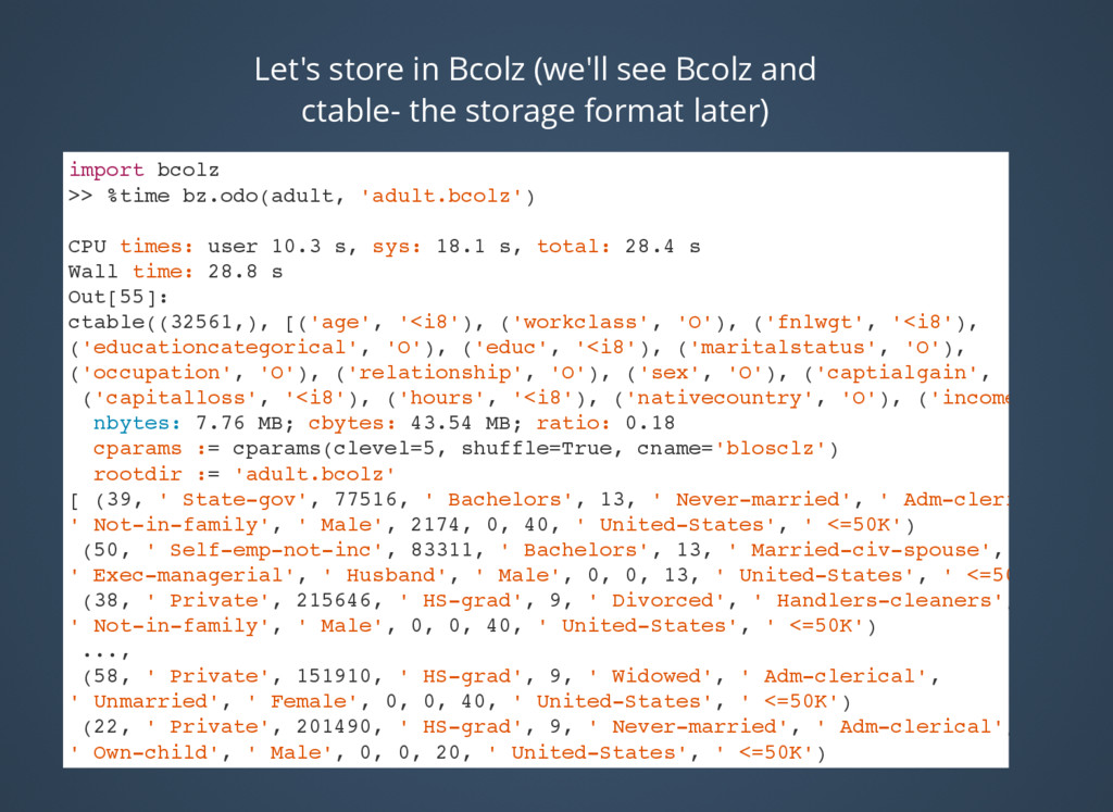
    ctable- the storage format later)
    import bcolz
    >> %time bz.odo(adult, 'adult.bcolz')
    CPU times: user 10.3 s, sys: 18.1 s, total: 28.4 s
    Wall time: 28.8 s
    Out[55]:
    ctable((32561,), [('age', '('educationcategorical', 'O'), ('educ', '('occupation', 'O'), ('relationship', 'O'), ('sex', 'O'), ('captialgain', '('capitalloss', 'nbytes: 7.76 MB; cbytes: 43.54 MB; ratio: 0.18
    cparams := cparams(clevel=5, shuffle=True, cname='blosclz')
    rootdir := 'adult.bcolz'
    [ (39, ' State-gov', 77516, ' Bachelors', 13, ' Never-married', ' Adm-clerical',
    ' Not-in-family', ' Male', 2174, 0, 40, ' United-States', ' <=50K')
    (50, ' Self-emp-not-inc', 83311, ' Bachelors', 13, ' Married-civ-spouse',
    ' Exec-managerial', ' Husband', ' Male', 0, 0, 13, ' United-States', ' <=50K')
    (38, ' Private', 215646, ' HS-grad', 9, ' Divorced', ' Handlers-cleaners',
    ' Not-in-family', ' Male', 0, 0, 40, ' United-States', ' <=50K')
    ...,
    (58, ' Private', 151910, ' HS-grad', 9, ' Widowed', ' Adm-clerical',
    ' Unmarried', ' Female', 0, 0, 40, ' United-States', ' <=50K')
    (22, ' Private', 201490, ' HS-grad', 9, ' Never-married', ' Adm-clerical',
    ' Own-child', ' Male', 0, 0, 20, ' United-States', ' <=50K')
    (52, ' Self-emp-inc', 287927, ' HS-grad', 9, ' Married-civ-spouse',
    

    View Slide

47. What else?
    What else?
    You can use any SQL supported by
    SQLAlchemy as your computation. It also
    supports Python lists, Spark DataFrames,
    MongoDB, Numpy arrays...
    

    View Slide

48. I want to maximize my
    I want to maximize my
    speed of reading/writing
    speed of reading/writing
    on a single computer
    on a single computer
    bcolz is a columnar data store for fast data storage
    and retrieval with built-in high performance
    compression. It supports both in-memory and out-
    of-memory storage and operations.
    Cf. .
    http://bcolz.blosc.org/
    

    View Slide

49. Bcolz
    Bcolz
    Fast IO and leverages Blosc for compression
    For certain problems like reading timeseries and
    doing analytics this can be useful
    We've seen immature projects like Castra built on top
    of it.
    We'll see more and more tools leveraging fast
    compression structures.
    Here I use POIWorld a dataset of 'Points of Interest'
    from OpenStreetMap
    Has some great synergies with binary formats like
    HDF5
    

    View Slide

50. df_poiworld = pd.read_csv('POIWorld.csv', usecols=columns)
    dc = bcolz.ctable.fromdataframe(df_poiworld)
    dc
    ctable((9140052,), [('name', 'O'), ('amenity', 'O'),
    ('Longitude', 'nbytes: 575.61 MB; cbytes: 3.00 GB; ratio: 0.19
    cparams := cparams(clevel=5, shuffle=True, cname='blosclz')
    [(nan, 'post_box', -0.20698000000000003, 51.9458753)
    (nan, 'post_box', -0.268633, 51.938183)
    (nan, 'post_box', -0.274278, 51.930209999999995) ...,
    (nan, nan, -77.2697855, 39.24023820000001)
    (nan, nan, -77.2777191, 39.237238399999995)
    (nan, 'drinking_water', -5.8, nan)]
    

    View Slide

51. >>> dc.cols
    age : carray((32561,), int64)
    nbytes: 254.38 KB; cbytes: 256.00 KB; ratio: 0.99
    cparams := cparams(clevel=5, shuffle=True, cname='blosclz')
    [39 50 38 ..., 58 22 52]
    workclass : carray((32561,), |S17)
    nbytes: 540.56 KB; cbytes: 303.83 KB; ratio: 1.78
    cparams := cparams(clevel=5, shuffle=True, cname='blosclz')
    [b' State-gov' b' Self-emp-not-inc' b' Private' ..., b' Private'
    b' Private' b' Self-emp-inc']
    educ : carray((32561,), int64)
    nbytes: 254.38 KB; cbytes: 256.00 KB; ratio: 0.99
    cparams := cparams(clevel=5, shuffle=True, cname='blosclz')
    [13 13 9 ..., 9 9 9]
    occupation : carray((32561,), |S18)
    nbytes: 572.36 KB; cbytes: 338.49 KB; ratio: 1.69
    cparams := cparams(clevel=5, shuffle=True, cname='blosclz')
    [b' Adm-clerical' b' Exec-managerial' b' Handlers-cleaners' ...,
    b' Adm-clerical' b' Adm-clerical' b' Exec-managerial']
    sex : carray((32561,), |S7)
    nbytes: 222.58 KB; cbytes: 256.00 KB; ratio: 0.87
    cparams := cparams(clevel=5, shuffle=True, cname='blosclz')
    [b' Male' b' Male' b' Male' ..., b' Female' b' Male' b' Female']
    hours : carray((32561,), int64)
    nbytes: 254.38 KB; cbytes: 256.00 KB; ratio: 0.99
    cparams := cparams(clevel=5, shuffle=True, cname='blosclz')
    [40 13 40 ..., 40 20 40]
    

    View Slide

52. %%time
    #Generate 1GB of data
    >> N = 100000 * 1000
    >> import bcolz
    >> ct = bcolz.fromiter(((i, i ** 2) for i in range(N)),
    dtype="i4, i8",
    count=N,
    cparams=bcolz.cparams(clevel=9))
    CPU times: user 59.6 s, sys: 1.08 s, total: 1min
    Wall time: 59.1 s
    >> ct
    ctable((100000000,), [('f0', 'nbytes: 1.12 GB; cbytes: 151.84 MB; ratio: 7.54
    cparams := cparams(clevel=9, shuffle=True, cname='blosclz')
    [(0, 0) (1, 1) (2, 4) ..., (99999997, 9999999400000009)
    (99999998, 9999999600000004) (99999999, 9999999800000001
    That is 7 times compression in-memory
    You can also store on disk and read it fast
    

    View Slide

53. >> %time ct.eval('f0 ** 2 + sqrt(f1)')
    CPU times: user 4.38 s, sys: 1.96 s, total: 6.34 s
    Wall time: 1.26 s
    Out[36]:
    carray((100000000,), float64)
    nbytes: 762.94 MB; cbytes: 347.33 MB; ratio: 2.20
    cparams := cparams(clevel=5, shuffle=True, cname='blosclz')
    [ 0.00000000e+00 2.00000000e+00 6.00000000e+00 ..., 1.37491943e+09
    1.57491943e+09 1.77491942e+09]
    Fast numerical calculations
    Integration with Numexpr to handle expressions
    Intelligent use of caching and multithreading to
    optimize numerical calcuations
    

    View Slide

54. Let's look at Adult dataset
    Let's look at Adult dataset
    again
    again
    With Bcolz you can do Pandas like things
    Based on NumPy but has support for PyTables/HDF5
    (which may be faster)
    Uses chunking. The chunked nature of bcolz objects,
    together with buffered I/O, makes appends very
    cheap
    This makes this ideal for say storing and retrieving
    market data.
    This is for fast fetch, and write rarely...
    

    View Slide

55. dc['workclass' == ' State-gov']
    #dc.cols
    # You can do DataFrame-like stuff
    dc['workclass' == ' State-gov']
    Out[117]:
    (39, b' State-gov', 13, b' Adm-clerical', b' Male', 40)
    PSA: Bcolz version 1 release candidate is out
    There are some challenges with integration into the rest of
    PyData, this should stabilize.
    

    View Slide

56. Quantopian Inc a crowd-sourced hedge fund uses Bcolz
    Each Column Is Stored Separately
    Escapes the GIL
    Better compression ratio for binary data
    Allows you to compress in-memory/ on disk and retrieve fast
    https://quantopian.github.io/talks/NeedForSpeed/slides.html
    

    View Slide

57. My data is bigger
    My data is bigger
    than RAM or in a
    than RAM or in a
    cluster
    cluster
    Use Dask or specifically
    Use Dask or specifically
    dask.array
    dask.array
    

    View Slide

58. Dask looks like this!
    Dask looks like this!
    Basically the
    Basically the
    Pandas/NumPy API
    Pandas/NumPy API
    import dask.array as da
    # create a dask array from the above array
    a2 = da.from_array(a, chunks=200)
    # multiply this array by a factor
    b2 = a2 * 4
    # find the minimum value
    b2_min = b2.min()
    print(b2_min)
    

    View Slide

59. #I want to tell if this is a School
    #or not and then plot it on a graph
    >> is_school = with_amenity.amenity.str.contains('[Ss]chool')
    >> school = with_amenity[is_school]
    #Very similar to pandas but you need to
    #call compute on the dask objects
    >> dd.compute(school.amenity.count())
    (342025,)
    # So we have about 342k schools in
    # UK and Ireland in the OpenStreetMap project
    

    View Slide

60. import dask.dataframe as dd
    lon, lat = dd.compute(school.Longitude,
    school.Latitude)
    import matplotlib.pyplot as plt
    from mpl_toolkits.basemap import Basemap
    fig, ax = plt.subplots(figsize=(10, 15))
    m = Basemap(projection='mill',
    lon_0=-5.23636, lat_0=53.866772,
    llcrnrlon=-10.65073, llcrnrlat=49.16209,
    urcrnrlon=1.76334, urcrnrlat=60.860699)
    m.drawmapboundary(fill_color='#ffffff', linewidth=.0)
    x, y = m(lon.values, lat.values)
    m.scatter(x, y, s=1, marker=',', color="steelblue", alpha=0.6);
    Compute in Dask and plot in Matplotlib
    Notice how similar to Pandas and NumPy
    the API is.
    

    View Slide

61. UK and Irish schools in Open Street Map
    

    View Slide

62. When do you use Dask?
    When do you use Dask?
    Medium data is greater than RAM size
    Generally Dask comes into it's own on around 16GB
    datasets
    Anything around the 1TB - 1PB range probably needs
    either a good SQL database or something like Spark
    Benchmark: My own Laptop has 4 cores and about
    8GB of RAM
    

    View Slide

63. Distributed Arrays
    Distributed Arrays
    - distributed arrays backed by Spark
    - other distributed arrays
    - another kind of distributed array (virtual)
    - Distributed arrays using task scheduling
    Bolt
    DistArray
    Biggus
    Dask.array
    

    View Slide

64. Very exciting technology for the JVM community
    Improvements in PySpark and interoperability
    Improvements in Machine Learning libraries
    Comes into it's own with lots of JSON blobs on
    many nodes
    Dramatic speed improvements for the 'easy to
    distribute' problems
    

    View Slide

65. Interlude
    Interlude
    

    View Slide

66. I want to speed up my code
    I want to speed up my code
    Numba (A fast LLVM based JIT compiler that is easy to use
    via decorators)
    Cython (A language that allows you to blend C objects for
    great speedup)
    PyPy (Another compiler but without support for NumPy
    code) Recent improvements in PyPy
    Plenty of tutorials online, and new tools are arriving...
    

    View Slide

67. End of Interlude
    End of Interlude
    

    View Slide

68. Recent improvements in
    Recent improvements in
    dealing with 'Big Data'
    dealing with 'Big Data'
    Distributed computing has improved in Dask
    See website
    PyData will just get better and better at dealing with
    'big data'
    Soon you may not need to use the JVM to deal with
    HDFS.
    Spark is improving too. Spark is very exciting and I
    could give an entire talk in Spark. Other people are
    doing that!
    Matt Rocklins
    

    View Slide

69. Arrow and Ibis
    Arrow and Ibis
    The project and
    This is combination of better SQL integration with the
    Pandas API and better columnar data structures for
    dealing with HDFS/Impala/ etc
    Arrow Ibis
    Source: Wes McKinney
    

    View Slide

70. Ibis Example
    Ibis Example
    rounds = con.table('pokemon_types')
    rounds.info()
    #This is a Pokemon table in SQLite
    rounds.slot.value_counts()
    slot count
    0 1 784
    1 2 395
    SQLite in the background but could be
    Impala - all with a pandas like API
    

    View Slide

71. PyData Map
    PyData Map
    https:/
    /peadarcoyle.wordpress.com/201
    https:/
    /peadarcoyle.wordpress.com/201
    6/03/02/a-map-of-the-pydata-stack/
    6/03/02/a-map-of-the-pydata-stack/
    Wouldn't it be great to have a map for the
    stack
    I had a a go
    

    View Slide

72. View Slide

73. I wanna do Stats/ML
    I wanna do Stats/ML
    There's lots of cool stuff in
    There's lots of cool stuff in
    PyData Land!
    PyData Land!
    

    View Slide

74. PyMC3
    PyMC3
    Recent improvements to documentation!!
    Written on top of Theano
    Timeseries examples, Bayesian Logistic Regression
    Model evaluation functions
    PSA: It's now in Beta
    

    View Slide

75. Bayesian LogReg
    Bayesian LogReg
    Subtitle
    Subtitle
    data[data['native-country']==" United-States"]
    income = 1 * (data['income'] == " >50K")
    age2 = np.square(data['age'])
    data = data[['age', 'educ', 'hours']]
    data['age2'] = age2
    data['income'] = income
    with pm.Model() as logistic_model:
    pm.glm.glm('income ~ age + age2 + educ + hours',
    data, family=pm.glm.families.Binomial())
    trace_logistic_model = pm.sample(2000,
    pm.NUTS(), progressbar=True)
    

    View Slide

76. Statsmodels
    Statsmodels
    PSA: If you want to help PyData a lot -
    PSA: If you want to help PyData a lot -
    work on Statsmodels
    work on Statsmodels
    

    View Slide

77. Scikit-Learn
    Scikit-Learn
    The best documentation in PyData
    Lots of cool improvements
    Chat to Andreas about this - he's at PyData
    Amsterdam
    

    View Slide

78. I want to analyze text
    I want to analyze text
    Production ready NLP toolkits all under open source
    

    View Slide

79. The future...
    The future...
    What is coming next
    What is coming next
    

    View Slide

80. Apache Arrow
    Apache Arrow
    Substantially improved data access speeds
    Closer to native performance Python extensions like
    Apache Spark
    New in-memory analytics functionality for
    nested/JSON-like data
    

    View Slide

81. Theano
    Theano
    Computational toolkits
    Computational toolkits
    Lasagne
    

    View Slide

82. So cite, send pull requests and/or help NumFOCUS!
    

    View Slide

83. View Slide