The Netflix Prize

Transcript

1. The Netflix Prize
   St. Louis Machine Learning
   August 22, 2012
   Steven Borrelli
   steve@borrelli.org
   @stevendborrelli {twitter, github}
   

   View Slide

2. The problem with recommendations?
   

   View Slide

3. • Founded 1997: DVDs rental by mail
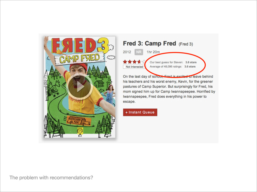
   • Users can rent as many movies per month, keep them without any late fees.
   But in order to get a new DVD they need to mail one back to Netflix.
   • Problem: most customers have a limited number of movies they know about
   or are interested in watching. This leads to customers quitting the service
   when they run out of films they want to request.
   • 1997-2000: No recommendation system (total catalog grows from 1k-5k
   movies)
   • 2000: Development of Cinematch Begins
   

   View Slide

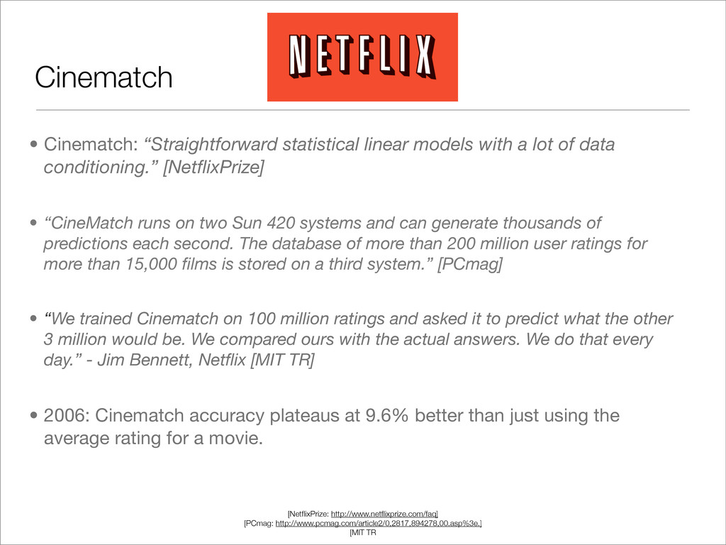
4. • Cinematch: “Straightforward statistical linear models with a lot of data
   conditioning.” [NetflixPrize]
   • “CineMatch runs on two Sun 420 systems and can generate thousands of
   predictions each second. The database of more than 200 million user ratings for
   more than 15,000 films is stored on a third system.” [PCmag]
   • “We trained Cinematch on 100 million ratings and asked it to predict what the other
   3 million would be. We compared ours with the actual answers. We do that every
   day.” - Jim Bennett, Netflix [MIT TR]
   • 2006: Cinematch accuracy plateaus at 9.6% better than just using the
   average rating for a movie.
   Cinematch
   [NetflixPrize: http://www.netflixprize.com/faq]
   [PCmag: http://www.pcmag.com/article2/0,2817,894278,00.asp%3e.]
   [MIT TR
   

   View Slide

5. The Netflix Prize
   

   View Slide

6. The Netflix Prize
   • Netflix to provide anonymized customer rating information
   • $1,000,000 to the competitor than can improve Cinematch by 10% on the
   same data set.
   • $50,000 annual “Progress Prize” for the system that most improves the
   accuracy of the last year’s winner.
   • Started October 2, 2006. If there is no winner, contest ends October 2, 2011.
   • Winners must describe to the world how their algorithm works.
   

   View Slide

7. The goal
   • Minimize RMSE = Root Mean Square Error
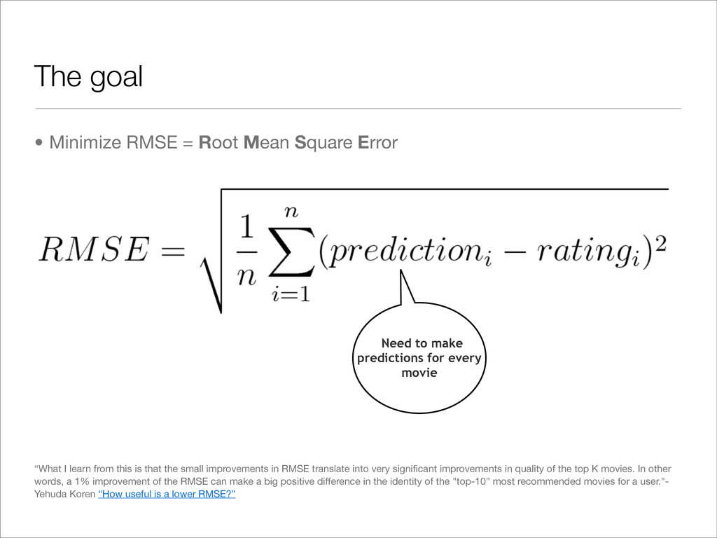
   “What I learn from this is that the small improvements in RMSE translate into very significant improvements in quality of the top K movies. In other
   words, a 1% improvement of the RMSE can make a big positive difference in the identity of the "top-10” most recommended movies for a user."-
   Yehuda Koren “How useful is a lower RMSE?”
   Need to make
   predictions for every
   movie
   

   View Slide

8. The goal
   Quiz Test
   Movie Average
   Cinematch
   Grand Prize
   1.0540
   0.9514 0.9525
   0.8563 0.8572
   

   View Slide

9. The Data
   

   View Slide

10. The Netflix Dataset
    • Number of Netflix customers in training set: 480,189
    • Training dataset: 100,480,507 ratings, scale of 1-5. The most recent 9
    ratings were taken and divided into three buckets:
    • Probe dataset: 1,408,395 ratings
    • Two Qualifying data sets: 2,817,131 ratings (divided 50-50 into quiz set and
    test set; quiz set results posted to Leaderboard)
    • Rating dates for training set: 10/98 to 12/05
    http://www.research.att.com/articles/featured_stories/2010_01/2010_02_netflix_article.html?fbid=gncVF5QUO56
    

    View Slide

11. The Netflix Dataset
    http://www.research.att.com/articles/featured_stories/2010_01/2010_02_netflix_article.html?fbid=gncVF5QUO56
    training set
    99,072,112 ratings
    17,770 files:
    Composed of
    ratings from users
    who made at least
    20 ratings
    Ratings Data Set
    104,706,033 entries
    probe set
    1,408,395 ratings
    rating, rating>
    quiz set
    1,408,342 entries
    rating>
    test set
    1,408,789 entries
    rating>
    Contestants use to
    test solution
    Used for
    leaderboard
    Used to
    determine
    winners
    Most recent 9
    ratings divided into
    three groups
    

    View Slide

12. Training vs. Probe
    http://www7.nationalacademies.org/cnstat/Bell%20Presentation.pdf
    

    View Slide

13. Differences between training and probe sets
    http://www.pitt.edu/~druzdzel/psfiles/zeszyty08.pdf
    

    View Slide

14. Time-dependent effects - weekdays
    http://www.pitt.edu/~druzdzel/psfiles/zeszyty08.pdf
    

    View Slide

15. Lessons:
    • Take time to understand the data
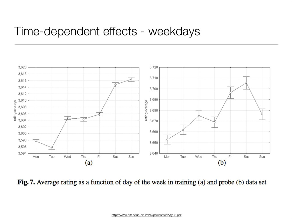
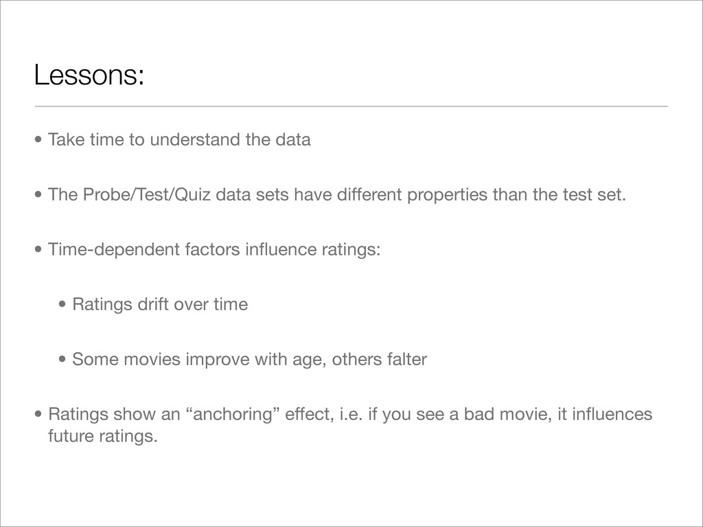
    • The Probe/Test/Quiz data sets have different properties than the test set.
    • Time-dependent factors influence ratings:
    • Ratings drift over time
    • Some movies improve with age, others falter
    • Ratings show an “anchoring” effect, i.e. if you see a bad movie, it influences
    future ratings.
    

    View Slide

16. Netflix Prize competition update
    

    View Slide

17. The Race
    • A week after the contest started, Cinematch had been beaten by 1%
    • Within a month, the lead had increased to almost 5%.
    • Several teams were early leaders:
    • WXYZConsulting, a team of Yi Zhang and Wei Xu. (A front runner during Nov-Dec 2006.)
    • ML@UToronto A, a team from the University of Toronto led by Prof. Geoffrey Hinton (A front runner during
    parts of Oct-Dec 2006.)
    • Gravity, a team of four scientists from the Budapest University of Technology (A front runner during Jan-May
    2007.)
    • BellKor, a group of scientists from AT&T Labs. (A front runner since May 2007.)
    http://www.cs.uic.edu/~liub/KDD-cup-2007/proceedings/The-Netflix-Prize-Bennett.pdf
    http://en.wikipedia.org/wiki/Netflix_Prize
    

    View Slide

18. Baseline Predictors
    

    View Slide

19. Baseline Predictors
    “...Typical collaborative filtering data exhibit large
    user and item biases – i.e., systematic tendencies for
    some users to give higher ratings than others, and
    for some items to receive higher ratings than
    others.” - Winning team’s 2009 GrandPrize Paper
    http://www.netflixprize.com/assets/GrandPrize2009_BPC_BellKor.pdf
    

    View Slide

20. Baseline Predictors
    bui = μ + bu + bi
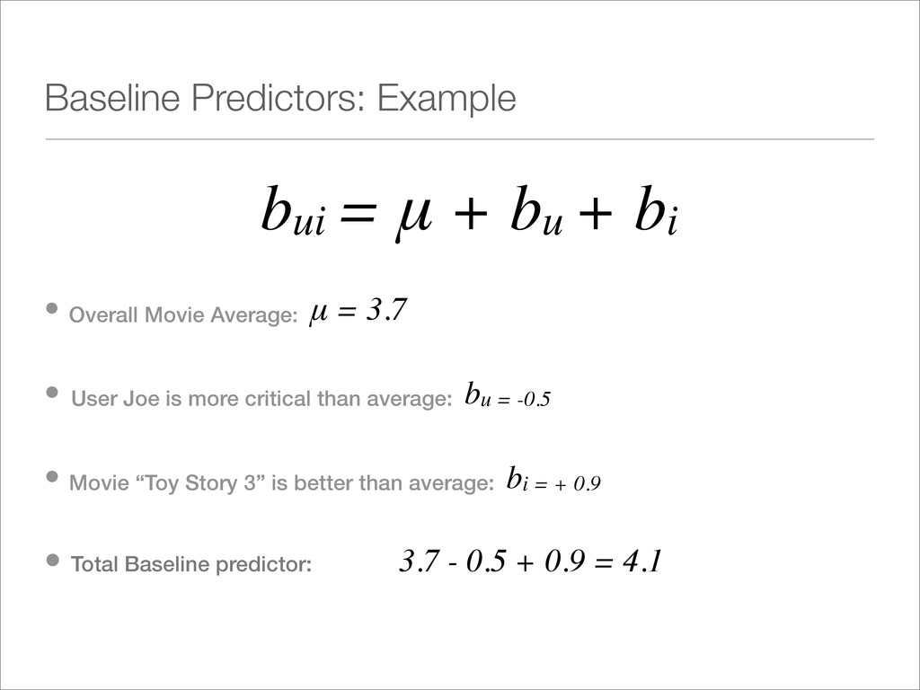
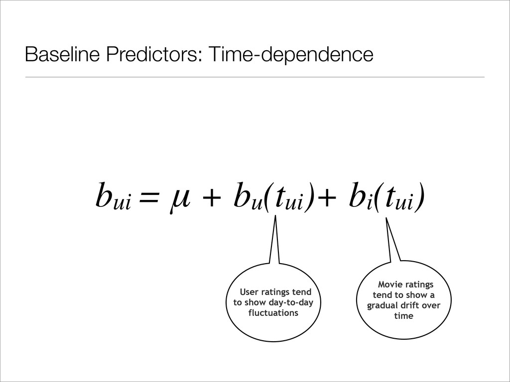
    Average rating for all
    movies (3.6)
    User bias (rates
    movies better/worse
    than other users)
    Movie bias (rated
    better/worse than
    other movies)
    Baseline prediction for
    user u on movie i.
    

    View Slide

21. Baseline Predictors: Example
    bui = μ + bu + bi
    • Overall Movie Average: μ = 3.7
    • User Joe is more critical than average: bu = -0.5
    • Movie “Toy Story 3” is better than average: bi = + 0.9
    • Total Baseline predictor: 3.7 - 0.5 + 0.9 = 4.1
    

    View Slide

22. Baseline Predictors: Time-dependence
    bui = μ + bu(tui)+ bi(tui)
    User ratings tend
    to show day-to-day
    fluctuations
    Movie ratings
    tend to show a
    gradual drift over
    time
    

    View Slide

23. Effect of baseline predictors
    Days since user’s 1st rating
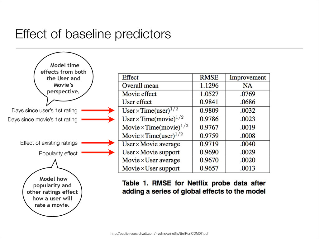
    Days since movie’s 1st rating
    Popularity effect
    Effect of existing ratings
    http://public.research.att.com/~volinsky/netflix/BellKorICDM07.pdf
    Model how
    popularity and
    other ratings effect
    how a user will
    rate a movie.
    Model time
    effects from both
    the User and
    Movie’s
    perspective.
    

    View Slide

24. Netflix Prize competition update
    

    View Slide

25. Progress Prize 2007
    • Won by KorBell/BellKor (AT&T) with an RMSE of 0.8712, 8.43% improvement
    • Blended 107 models, used SVD and RBM to model latent factors.
    http://www.cs.uic.edu/~liub/KDD-cup-2007/proceedings/The-Netflix-Prize-Bennett.pdf
    http://en.wikipedia.org/wiki/Netflix_Prize
    

    View Slide

26. Collaborative Filtering: latent factors
    

    View Slide

27. User/Movie Ratings Matrix
    1
    4
    3 2
    4
    5 5
    4
    3
    1
    4
    n movies (~ 18,000)
    m users (~ 480,000)
    • 480,000 * 18000 ~ 8.5 billion entries
    • Only have 100 million ratings
    • Matrix is 98.8% empty.
    • Goal is develop a model for the
    missing ratings.
    

    View Slide

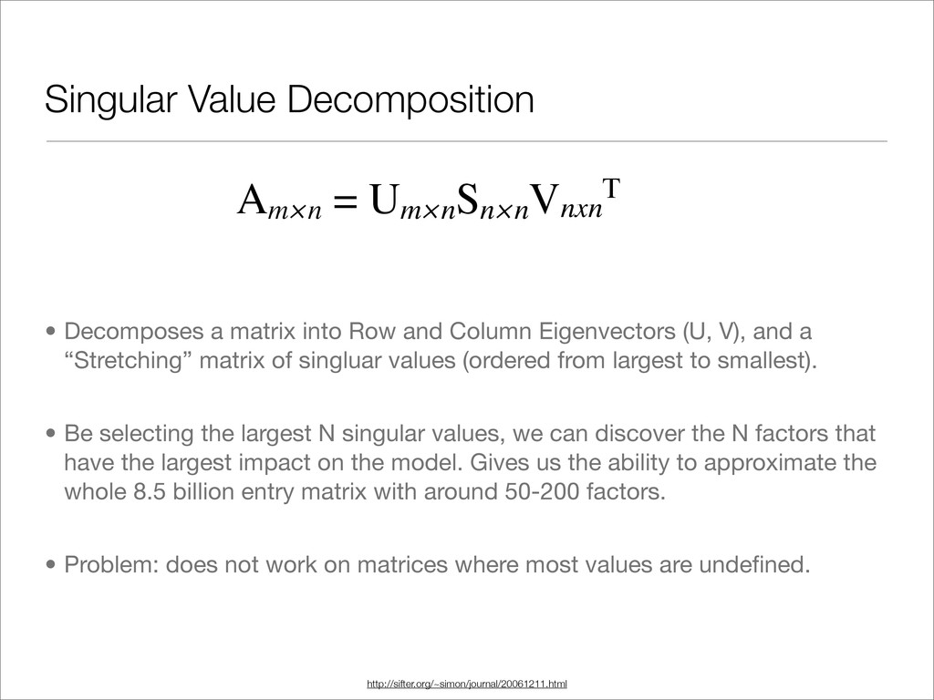
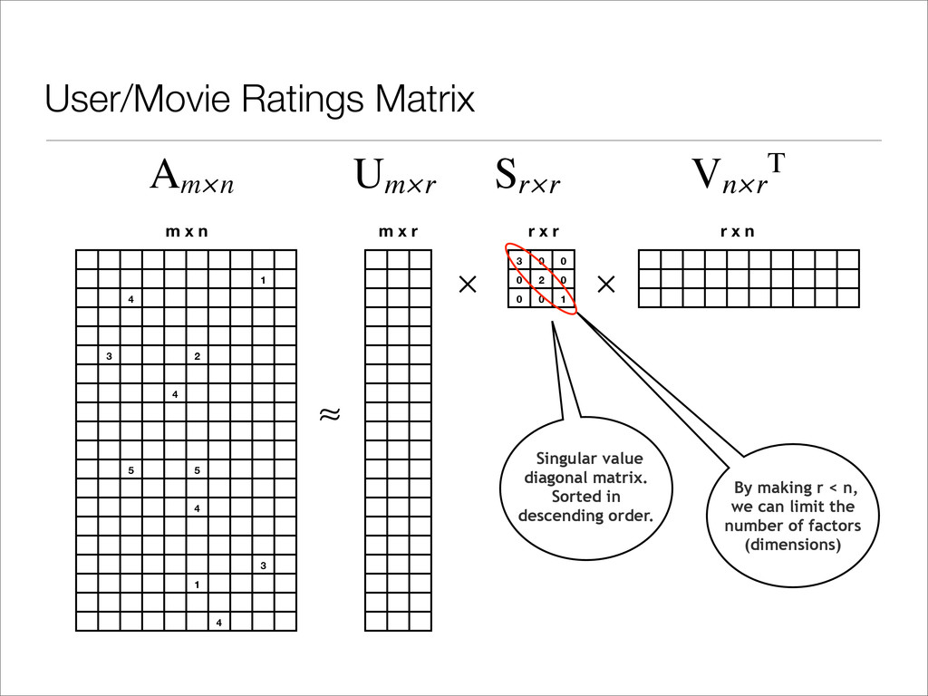
28. • Decomposes a matrix into Row and Column Eigenvectors (U, V), and a
    “Stretching” matrix of singluar values (ordered from largest to smallest).
    • Be selecting the largest N singular values, we can discover the N factors that
    have the largest impact on the model. Gives us the ability to approximate the
    whole 8.5 billion entry matrix with around 50-200 factors.
    • Problem: does not work on matrices where most values are undefined.
    Singular Value Decomposition
    http://sifter.org/~simon/journal/20061211.html
    Am×n
    = Um×n
    Sn×n
    Vnxn
    T
    

    View Slide

29. User/Movie Ratings Matrix
    1
    4
    3 2
    4
    5 5
    4
    3
    1
    4
    m x n
    3 0 0
    0 2 0
    0 0 1
    m x r r x r r x n
    ×
    ≈
    ×
    Singular value
    diagonal matrix.
    Sorted in
    descending order.
    Am×n
    Um×r
    Sr×r
    Vn×r
    T
    By making r < n,
    we can limit the
    number of factors
    (dimensions)
    

    View Slide

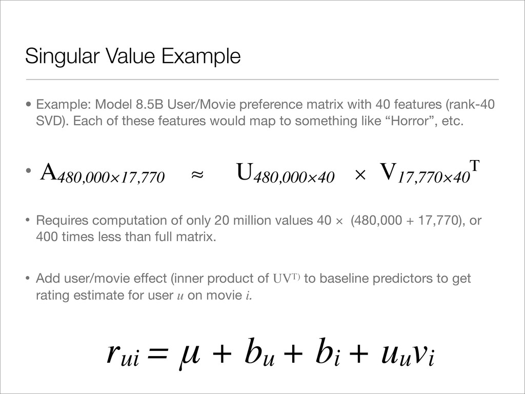
30. • Example: Model 8.5B User/Movie preference matrix with 40 features (rank-40
    SVD). Each of these features would map to something like “Horror”, etc.
    • A480,000×17,770
    U480,000×40
    V17,770×40
    T
    • Requires computation of only 20 million values 40 × (480,000 + 17,770), or
    400 times less than full matrix.
    • Add user/movie effect (inner product of UVT) to baseline predictors to get
    rating estimate for user u on movie i.
    rui = μ + bu + bi + uuvi
    Singular Value Example
    ≈ ×
    

    View Slide

31. Simon Funk: Breakthrough in SVD
    http://sifter.org/~simon/journal/20061211.html
    

    View Slide

32. Incremental SVD
    • Select R number of features to use. Run calculations on existing ratings.
    Learning rate discovered through testing.
    • Incremental gradient descent: follow steepest descent of the partial derivative
    of the error, which is a simple equation.
    /*
    * Where:
    * real *userValue = userFeature[featureBeingTrained];
    * real *movieValue = movieFeature[featureBeingTrained];
    * real lrate = 0.001;
    */
    static inline
    void train(int user, int movie, real rating)
    {
    real err = lrate * (rating - predictRating(movie, user));
    userValue[user] += err * movieValue[movie];
    movieValue[movie] += err * userValue[user];
    }
    http://www.infosci.cornell.edu/courses/info4300/2011fa/slides/08.pdf
    

    View Slide

33. Conditional Restricted Boltzmann Machine
    Implicit
    binary vector: 1
    if user rated movie
    (we can get value
    out of quiz/test
    data!)
    http://www.machinelearning.org/proceedings/icml2007/papers/407.pdf
    Rating binary
    vector: position is set
    to 1 to match user
    rating (i.e., 3)
    Hidden factors we
    are trying to learn.
    Factors could
    be children’s
    movies, sci-fi, or
    international
    films.
    

    View Slide

34. • Start with a training vector on the visible units.
    • Update states on hidden units in parallel using logistic activation.
    • Use hidden units to reconstruct visible units in parallel.
    Daydreaming RBMS
    http://www.cs.toronto.edu/~hinton/absps/guideTR.pdf
    h1 h2 h3
    h1 h2 h3
    h1 h2 h3
    v1 v2 v3
    v1 v2 v3
    v1 v2 v3
    v1 v2 v3
    t0
    t0
    t1
    t1 tn-1
    t2 tn
    0 n
    

    View Slide

35. Collaborative Filtering: neighborhood models
    

    View Slide

36. View Slide

37. Netflix Prize competition update
    

    View Slide

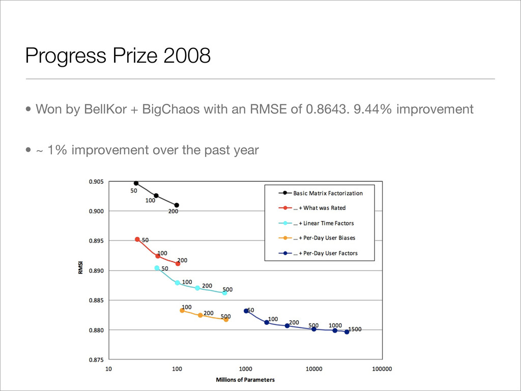
38. • Won by BellKor + BigChaos with an RMSE of 0.8643. 9.44% improvement
    • ~ 1% improvement over the past year
    Progress Prize 2008
    http://www.cs.uic.edu/~liub/KDD-cup-2007/proceedings/The-Netflix-Prize-Bennett.pdf
    http://en.wikipedia.org/wiki/Netflix_Prize
    

    View Slide

39. Ensemble methods
    

    View Slide

40. Technique Distribution
    

    View Slide

41. Ensemble Methods
    • “..using increasingly complex models is only one way of improving accuracy.
    An apparently easier way to achieve better accuracy is by blending multiple
    simpler models.” - BellKor 2008 Progress Prize Solution
    • Combine model predictions: a blended collection of simple models is often
    more accurate than a single complex one.
    

    View Slide

42. • Linear Model Blend: w = (XT X + λI)−1XT y (standard least squares solutions)
    • Neural Network Blending
    Ensemble Methods
    

    View Slide

43. • Gradient Boosted Decision Trees:
    • Each cell represents a simple decision tree. The tree on the left trains on the
    raw data. The second tree trains on the residual error of the first; the third tree
    on the residuals of the second and so on.
    • Grand prize winners blended over 800 models.
    Ensemble Methods
    

    View Slide

44. Lessons:
    • Use latent factorization methods to learn dimensions of the problem
    • Use regularization at every step to reduce overfitting. Learn regularization
    weights through trial and error.
    • Use neighborhood models (k-NN) in combination with latent factors. Take into
    account relevance of neighbor’s effects. If local similarity is weak, use global
    factors.
    • Single models hit an accuracy wall, combining predictors can increase
    accuracy.
    

    View Slide

45. The Finale
    

    View Slide

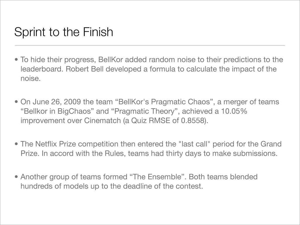
46. • To hide their progress, BellKor added random noise to their predictions to the
    leaderboard. Robert Bell developed a formula to calculate the impact of the
    noise.
    • On June 26, 2009 the team “BellKor's Pragmatic Chaos”, a merger of teams
    “Bellkor in BigChaos” and “Pragmatic Theory”, achieved a 10.05%
    improvement over Cinematch (a Quiz RMSE of 0.8558).
    • The Netflix Prize competition then entered the "last call" period for the Grand
    Prize. In accord with the Rules, teams had thirty days to make submissions.
    • Another group of teams formed “The Ensemble”. Both teams blended
    hundreds of models up to the deadline of the contest.
    Sprint to the Finish
    

    View Slide

47. http://www.research.att.com/articles/featured_stories/2010_05/201005_netflix2_article.html?fbid=gncVF5QUO56
    

    View Slide

48. View Slide

49. View Slide

50. The Napoleon Dynamite Problem
    • Frequently rated movies with polarized ratings.
    http://whimsley.typepad.com/whimsley/2009/10/netflix-prize-was-the-napoleon-dynamite-problem-solved.html
    100K+ Ratings
    1.1934 RMSE
    

    View Slide

51. Aftermath
    

    View Slide

52. Aftermath
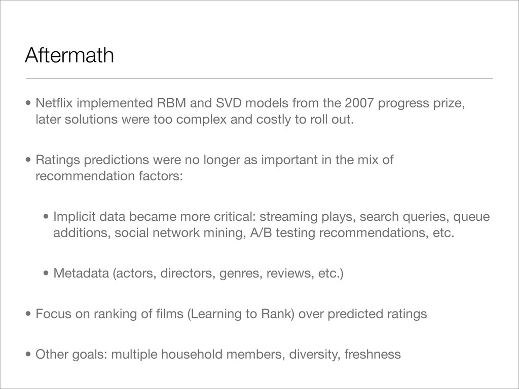
    • Netflix implemented RBM and SVD models from the 2007 progress prize,
    later solutions were too complex and costly to roll out.
    • Ratings predictions were no longer as important in the mix of
    recommendation factors:
    • Implicit data became more critical: streaming plays, search queries, queue
    additions, social network mining, A/B testing recommendations, etc.
    • Metadata (actors, directors, genres, reviews, etc.)
    • Focus on ranking of films (Learning to Rank) over predicted ratings
    • Other goals: multiple household members, diversity, freshness
    

    View Slide

53. Where to go next
    • Try a contest! http://kaggle.com
    • Sources for the presentation: http://borrelli.org/2012/08/11/netflix-prize-links/
    • There are a tremendous amount of open-source tools available:
    • RStudio: http://www.rstudio.org/
    • Python Scikit-Learn: http://scikit-learn.org/stable/
    • Apache Mahout: http://mahout.apache.org
    

    View Slide

54. Thank you for coming!
    

    View Slide