California Institute of Technology. Government sponsorship acknowledged Stephen R. Taylor Bayesian model-emulation of GW spectra for probes of the final-parsec problem with pulsar-timing arrays JET PROPULSION LABORATORY, CALIFORNIA INSTITUTE OF TECHNOLOGY Joseph Simon (UWM), Laura Sampson (CIERA, Northwestern University)
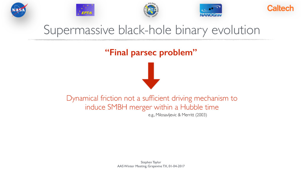
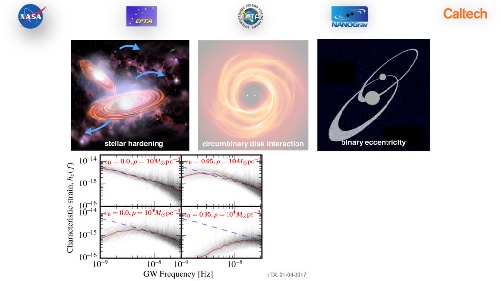
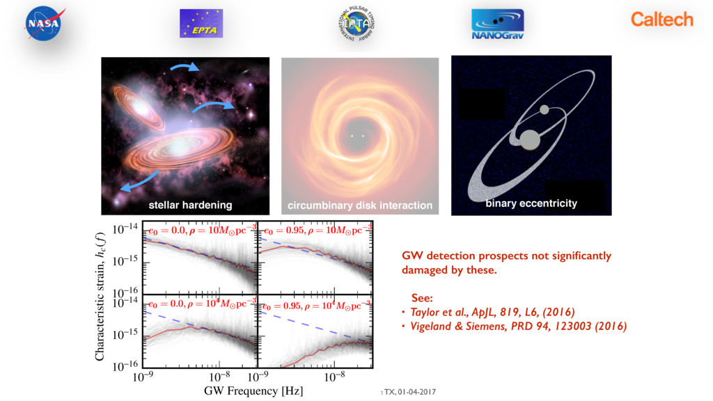
problem” Dynamical friction not a sufficient driving mechanism to induce SMBH merger within a Hubble time e.g., Milosavljevic & Merritt (2003) Supermassive black-hole binary evolution
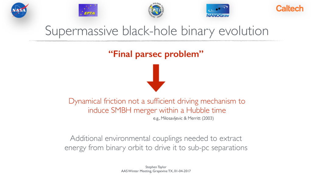
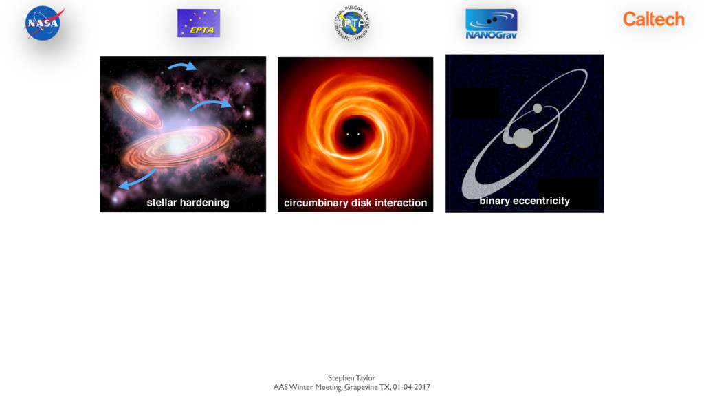
problem” Dynamical friction not a sufficient driving mechanism to induce SMBH merger within a Hubble time e.g., Milosavljevic & Merritt (2003) Additional environmental couplings needed to extract energy from binary orbit to drive it to sub-pc separations Supermassive black-hole binary evolution
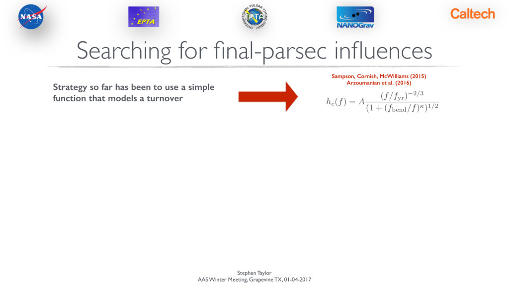
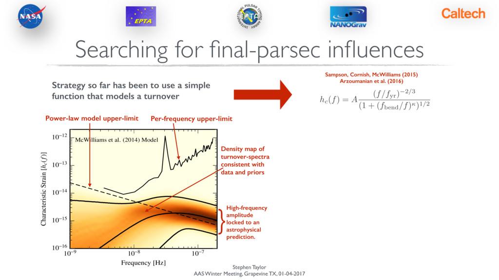
final-parsec influences hc(f) = A (f/fyr) 2/3 (1 + (fbend/f))1/2 Sampson, Cornish, McWilliams (2015) Arzoumanian et al. (2016) Strategy so far has been to use a simple function that models a turnover
final-parsec influences 12 10-9 10-8 10-7 Frequency [Hz] 10-16 10-15 10-14 10-13 10-12 Characteristic Strain [hc(f)] McWilliams et al. (2014) Model hc(f) = A (f/fyr) 2/3 (1 + (fbend/f))1/2 Sampson, Cornish, McWilliams (2015) Arzoumanian et al. (2016) Strategy so far has been to use a simple function that models a turnover Per-frequency upper-limit Power-law model upper-limit Density map of turnover-spectra consistent with data and priors }High-frequency amplitude locked to an astrophysical prediction.
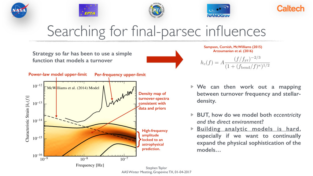
final-parsec influences 12 10-9 10-8 10-7 Frequency [Hz] 10-16 10-15 10-14 10-13 10-12 Characteristic Strain [hc(f)] McWilliams et al. (2014) Model hc(f) = A (f/fyr) 2/3 (1 + (fbend/f))1/2 Sampson, Cornish, McWilliams (2015) Arzoumanian et al. (2016) ! We can then work out a mapping between turnover frequency and stellar- density. ! BUT, how do we model both eccentricity and the direct environment? Building analytic models is hard, especially if we want to continually expand the physical sophistication of the models… Strategy so far has been to use a simple function that models a turnover Per-frequency upper-limit Power-law model upper-limit Density map of turnover-spectra consistent with data and priors }High-frequency amplitude locked to an astrophysical prediction.
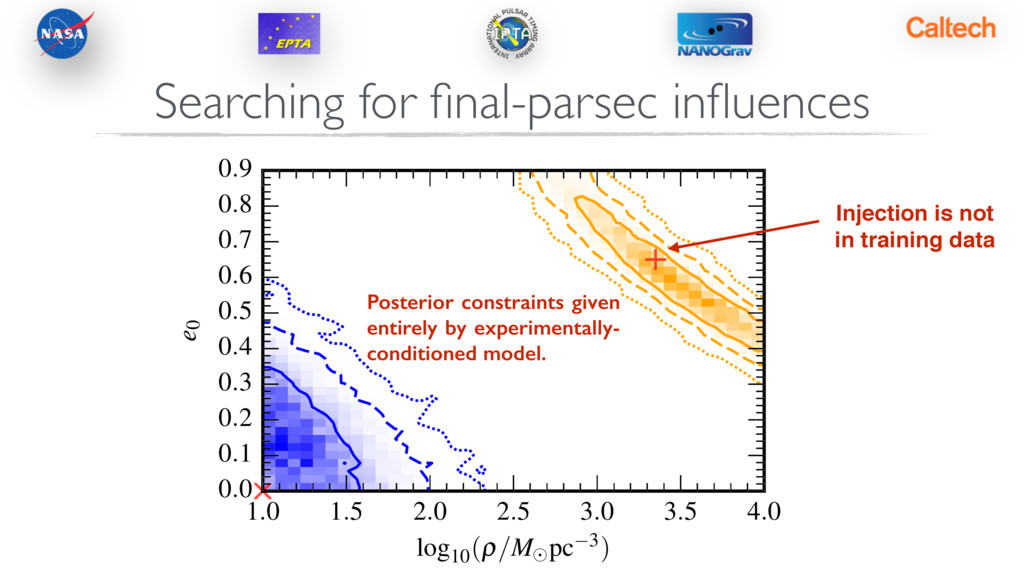
emulation Run a small number of expensive SMBHB population simulations. Train a Gaussian process to learn the shape of the spectrum. Learn the spectral variance due to finiteness of the SMBHB population. ! We have a predictor for the shape of the spectrum, AND a measure of the uncertainty from the interpolation scheme. Searching for final-parsec influences
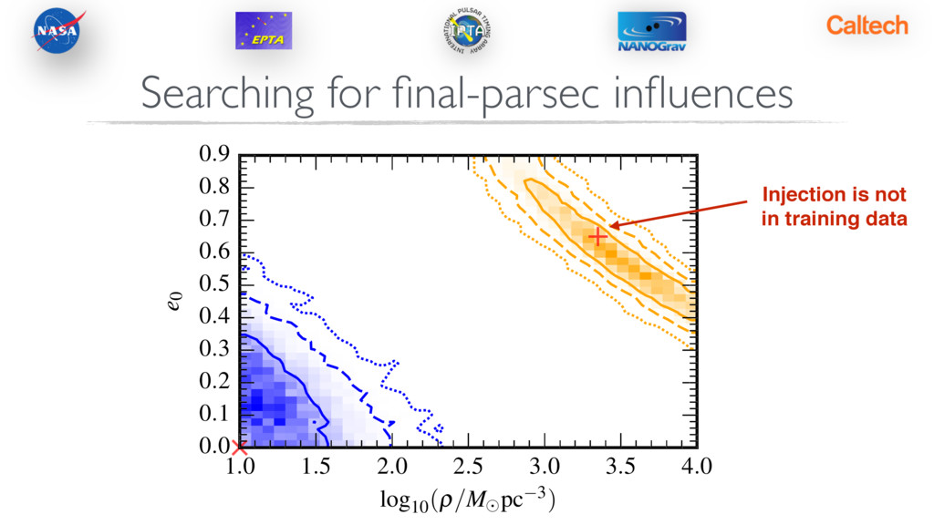
final-parsec influences 1.0 1.5 2.0 2.5 3.0 3.5 4.0 log10 (r/M pc 3) 0.0 0.1 0.2 0.3 0.4 0.5 0.6 0.7 0.8 0.9 e0 Injection is not ! in training data ! Posterior constraints given entirely by experimentally- conditioned model.
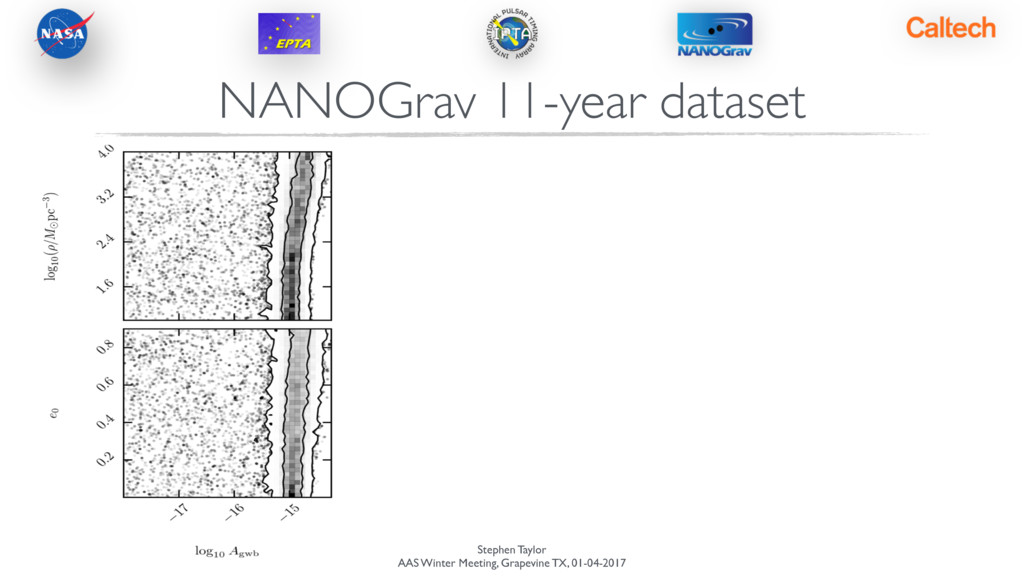
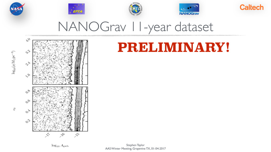
dataset PRELIMINARY! There are (very) early hints of a low-frequency process that is common to all NANOGrav pulsars. ! This could have a variety of sources, including (but not limited to) a GW background. ! As such, we can attempt dynamical constraints without anchoring the high-frequency strain amplitude with a prior. ! Dynamical constraints are weak, but there are some subtle signs of covariance between the high-frequency amplitude and the eccentricity/stellar-density.
history of SMBHBs is encoded in the strain spectrum of GWs in the PTA band. ! We can now build physically-sophisticated spectral models by training Gaussian Processes on simulated populations of binaries. Sometimes its easier to simulate the Universe than write down an equation. ! “Constraints On The Dynamical Environments Of Supermassive Black- hole Binaries Using Pulsar-timing Arrays”, Taylor, Simon, Sampson, arXiv:1612.02817 ! This approach can be adapted for LIGO and LISA population inference, to map from distributions of source properties back to progenitor characteristics.