Government sponsorship acknowledged Stephen R. Taylor Introduction To NANOGrav Data Analysis JET PROPULSION LABORATORY, CALIFORNIA INSTITUTE OF TECHNOLOGY
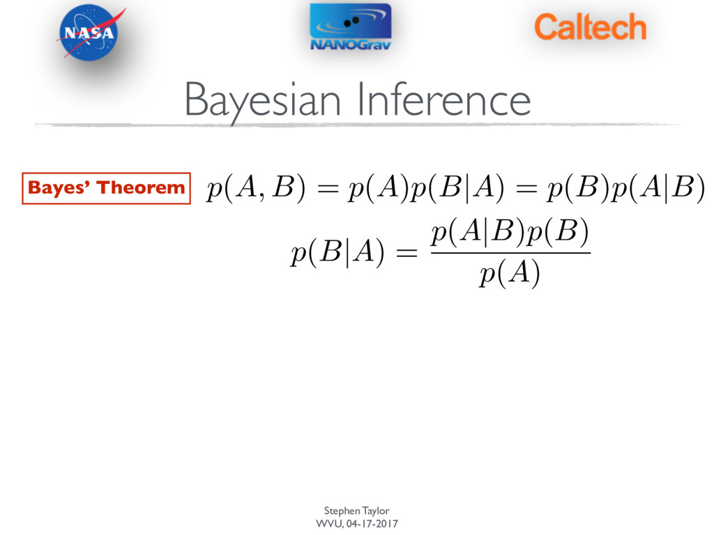
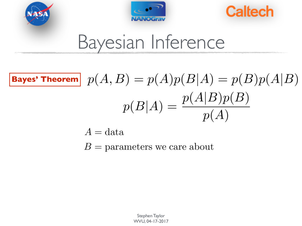
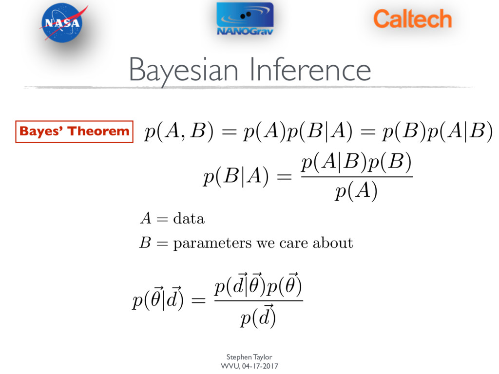
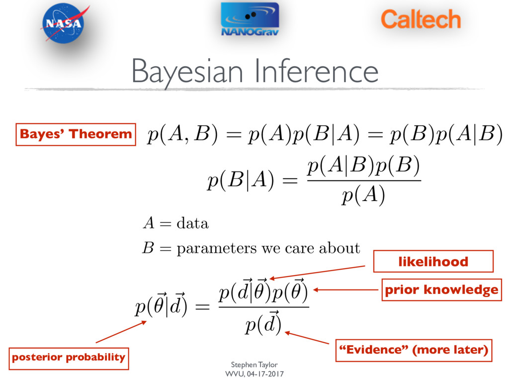
= p(B)p(A|B) p(B|A) = p(A|B)p(B) p(A) Bayes’ Theorem A = data B = parameters we care about p(~ ✓|~ d) = p(~ d|~ ✓)p(~ ✓) p(~ d) posterior probability likelihood prior knowledge “Evidence” (more later)
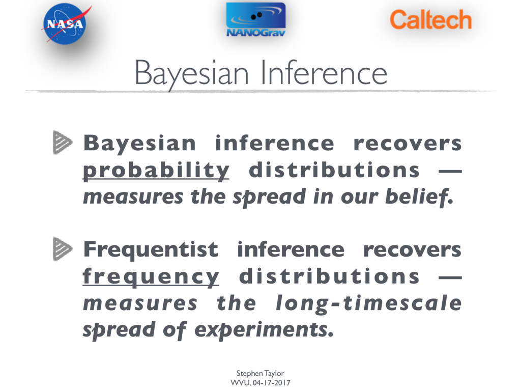
distributions — measures the spread in our belief. Frequentist inference recovers frequency distributions — measures the long-timescale spread of experiments.
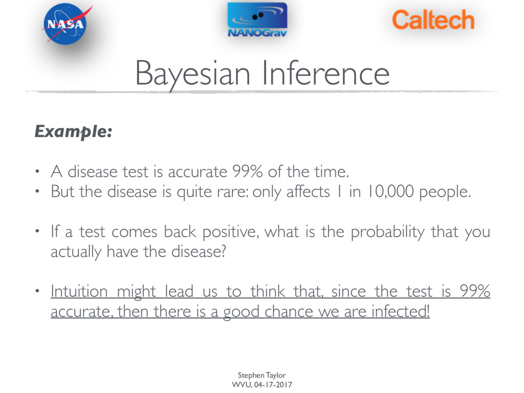
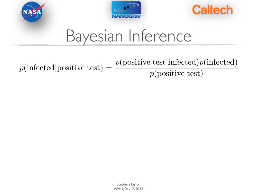
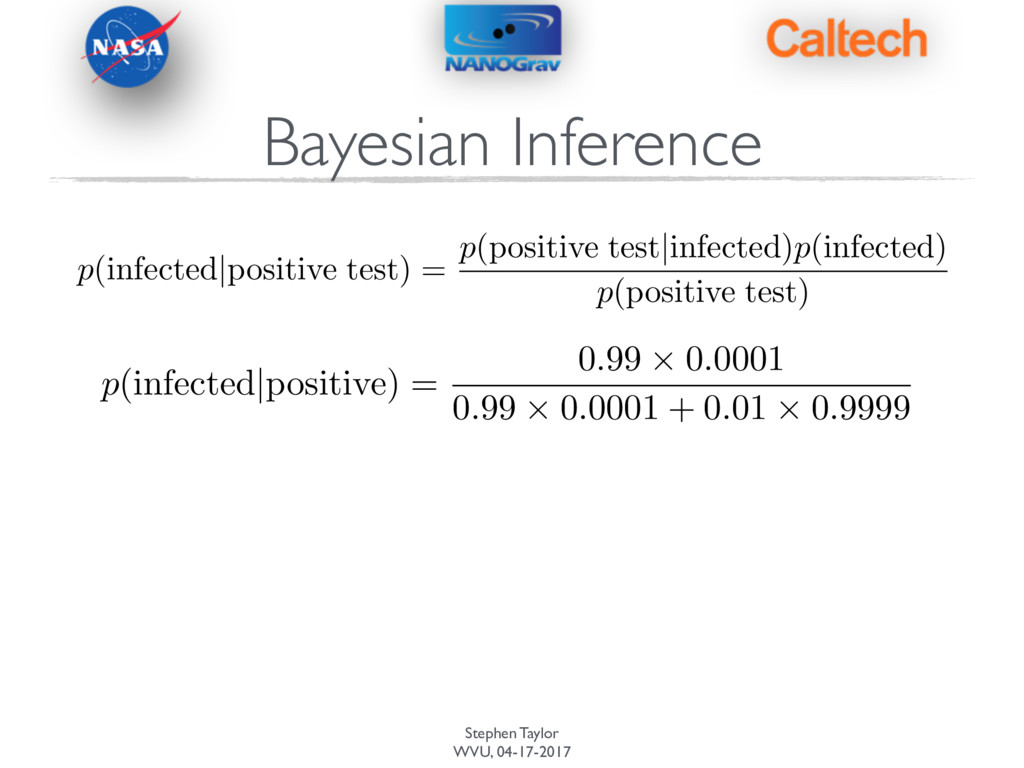
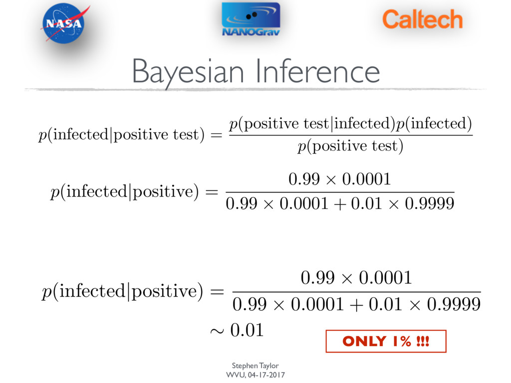
test is accurate 99% of the time. • But the disease is quite rare: only affects 1 in 10,000 people. • If a test comes back positive, what is the probability that you actually have the disease? • Intuition might lead us to think that, since the test is 99% accurate, then there is a good chance we are infected!
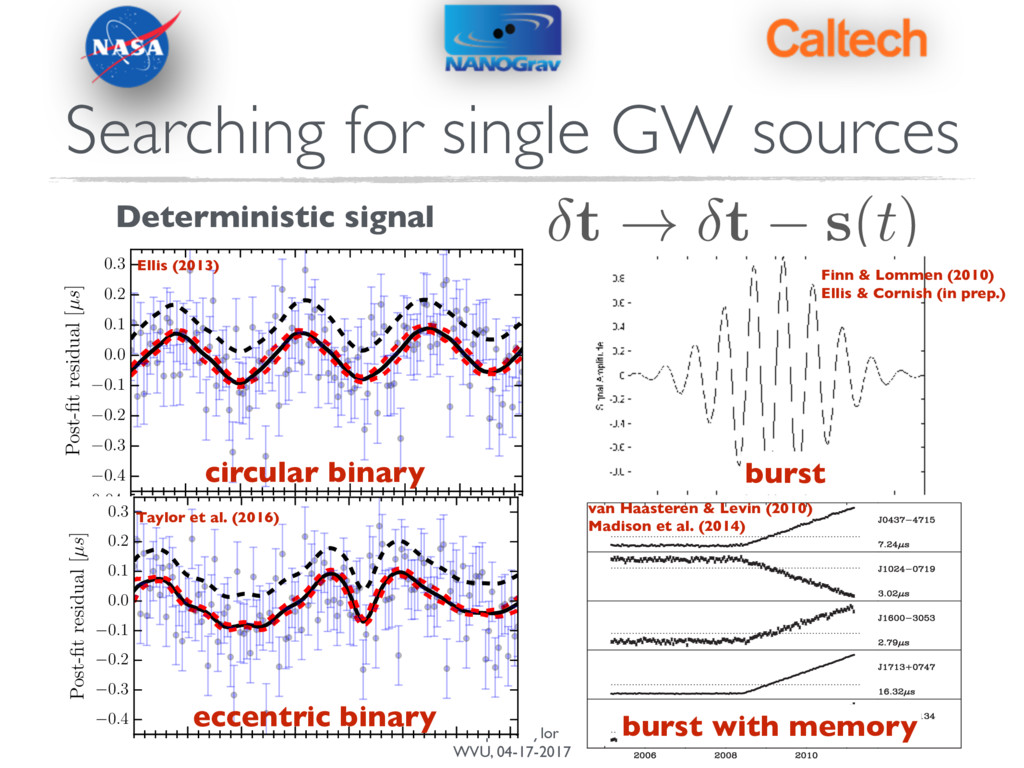
of signals • (1) stochastic — characterize through statistical properties, e.g. standard deviation • (2) deterministic — characterize through amplitude, phase, etc.
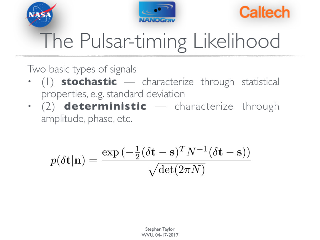
of signals • (1) stochastic — characterize through statistical properties, e.g. standard deviation • (2) deterministic — characterize through amplitude, phase, etc. p ( t|n ) = exp ( 1 2 ( t s ) T N 1 ( t s )) p det(2 ⇡N )
of signals • (1) stochastic — characterize through statistical properties, e.g. standard deviation • (2) deterministic — characterize through amplitude, phase, etc. p ( t|n ) = exp ( 1 2 ( t s ) T N 1 ( t s )) p det(2 ⇡N ) The only difference between treating stochastic signals and deterministic signals is through our prior on s
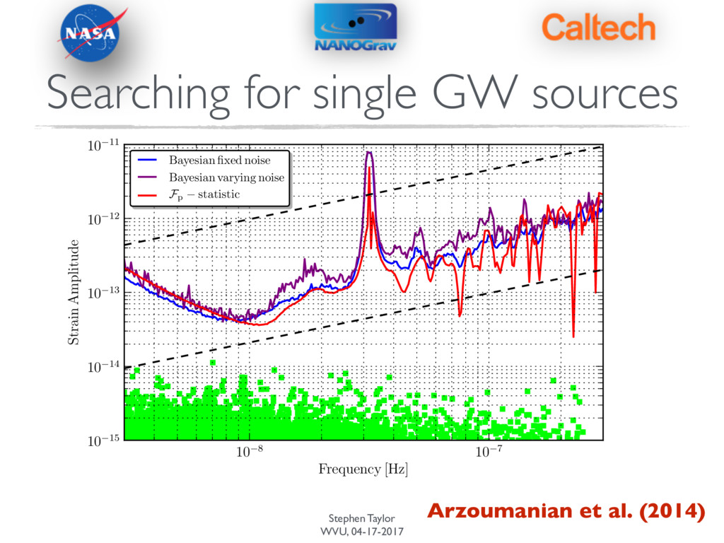
[Hz] 10 15 10 14 10 13 10 12 10 11 Strain Amplitude Bayesian fixed noise Bayesian varying noise Fp statistic Figure 5. Sky-averaged upper limit on the strain amplitude, h 0 as a function of GW frequency. The Bayesian upper limits are computed using a fixed-noise model (thick black(blue)) and a varying noise model (thin black(purple)) and the frequentist upper limit (gray(red)) is computed using the Fp-statistic. The dashed curves indicate lines of constant chirp mass for a source with a distance to the Virgo cluster (16.5 Mpc) and chirp mass of 109M (lower) and 1010M (upper). The gray(green) squares show the strain amplitude of the loudest GW sources in 1000 monte-carlo realizations using an optimistic phenomenological Arzoumanian et al. (2014) Searching for single GW sources
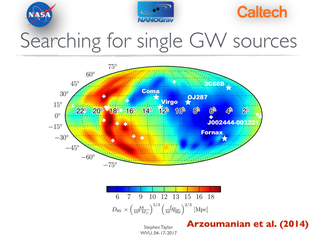
⌘5/3 ⇣ fgw 10 8Hz ⌘2/3 [Mpc] Figure 6. 95% lower limit on the luminosity distance as a function of sky location computed using the Fp-statistic plotted in equatorial coordinates . The values in the colorbar are calculated assuming a chirp mass of M = 109M and a GW frequency f gw = 1 ⇥ 10-8 Hz. The white diamonds denote the locations of the pulsars in the sky and the black(white) stars denote possible SMBHBs or clusters possibly containing SMBHBs. As expected from the antenna pattern functions of the pulsars, we are most sensitive to GWs from sky locations near the pulsars. The luminosity distances to the potential sources are 92.3, 1575.5, 2161.7, 16.5, 104.5, and 19 Mpc for 3C66B, OJ287, J002444-003221, Virgo Cluster, Coma Cluster, and Fornax Cluster, respectively. (Color figure available in the online version.) 6 7 9 10 12 13 15 16 18 D95 ⇥ ⇣ M 109 M ⌘5/3 ⇣ fgw 10 8Hz ⌘2/3 [Mpc] Coma Virgo OJ287 Fornax 3C66B J002444-003221 Figure 7. 95% lower limit on the luminosity distance as a function of sky location computed using the Bayesian method including the noise model. The values in the colorbar are calculated assuming a chirp mass of M = 109M and a GW frequency f gw = 1 ⇥ 10-8 Hz. The white diamonds denote the locations of the Arzoumanian et al. (2014) Searching for single GW sources
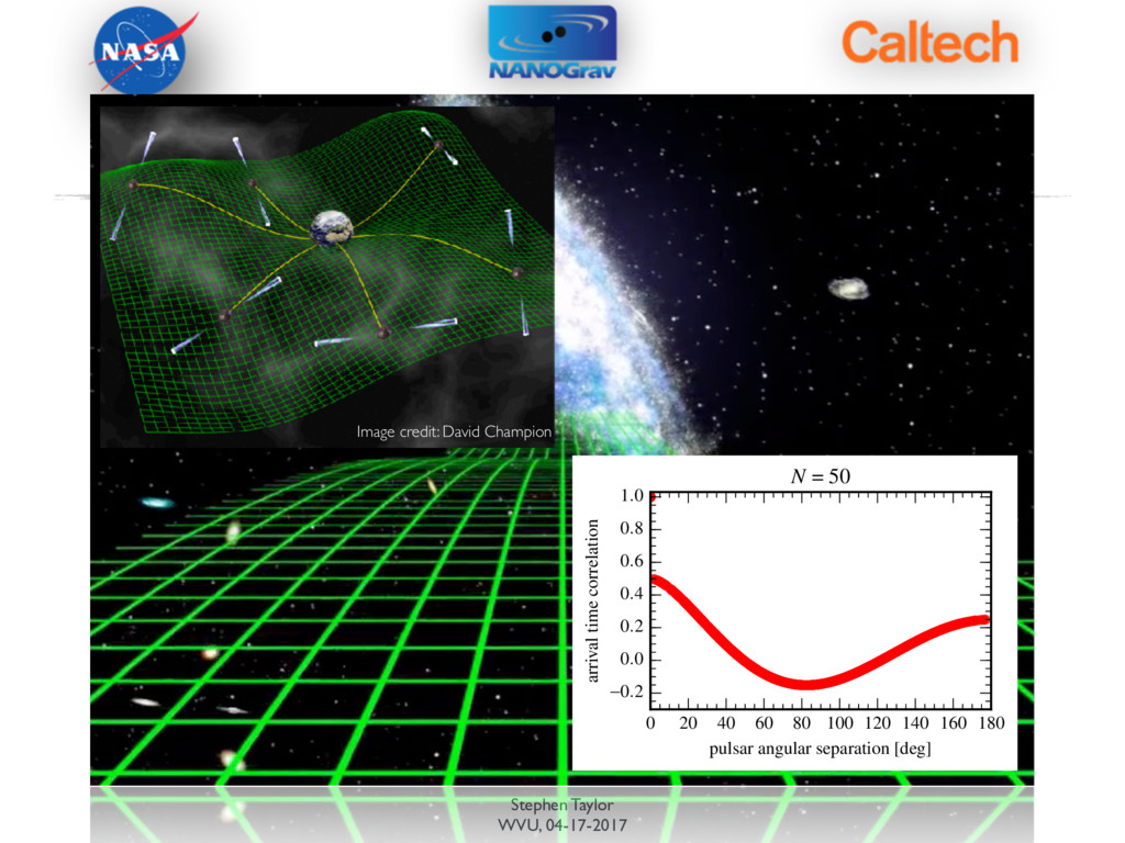
We have lots of binaries, so we can’t track all of them. • Look at statistical properties of the signal, e.g. the variance. • All information on the background is in signal variance and cross correlations between pulsars.
We have lots of binaries, so we can’t track all of them. • Look at statistical properties of the signal, e.g. the variance. • All information on the background is in signal variance and cross correlations between pulsars.
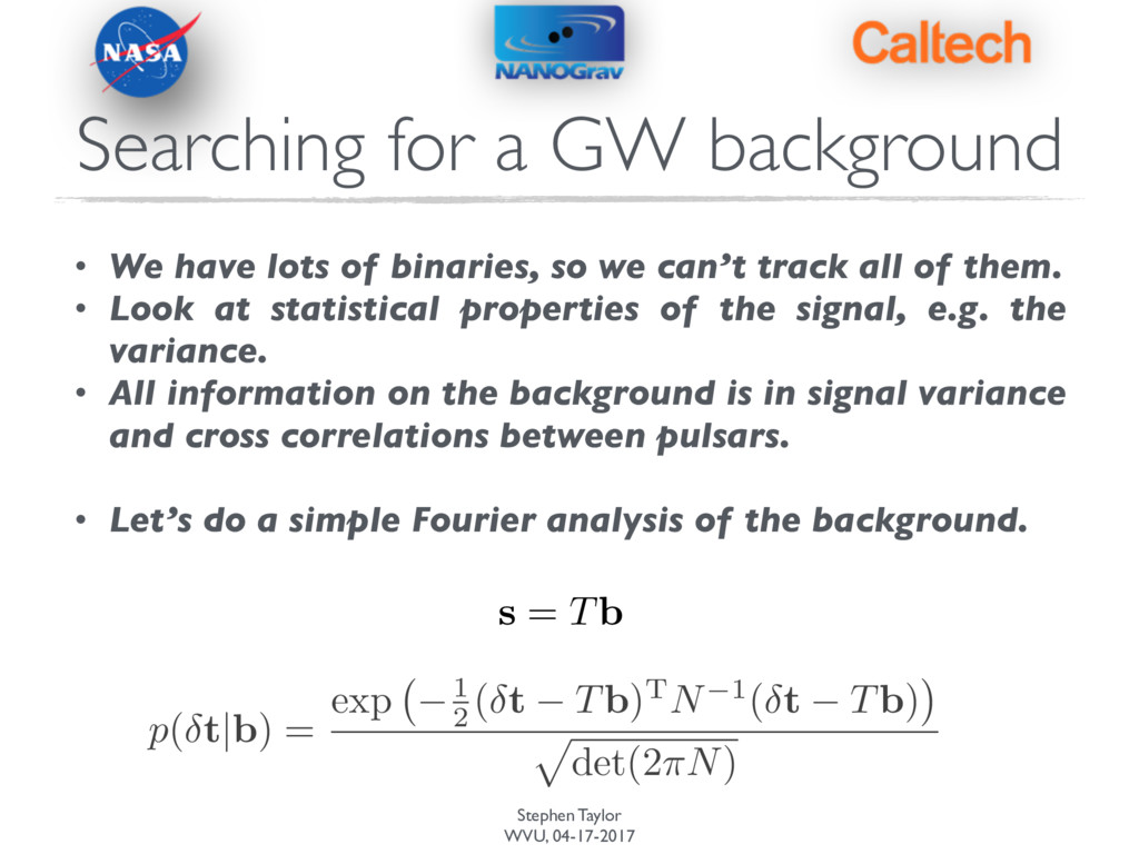
We have lots of binaries, so we can’t track all of them. • Look at statistical properties of the signal, e.g. the variance. • All information on the background is in signal variance and cross correlations between pulsars. • Let’s do a simple Fourier analysis of the background.
We have lots of binaries, so we can’t track all of them. • Look at statistical properties of the signal, e.g. the variance. • All information on the background is in signal variance and cross correlations between pulsars. • Let’s do a simple Fourier analysis of the background. s = Tb
1 2 ( t Tb ) TN 1 ( t Tb ) p det(2 ⇡N ) Searching for a GW background • We have lots of binaries, so we can’t track all of them. • Look at statistical properties of the signal, e.g. the variance. • All information on the background is in signal variance and cross correlations between pulsars. • Let’s do a simple Fourier analysis of the background. s = Tb
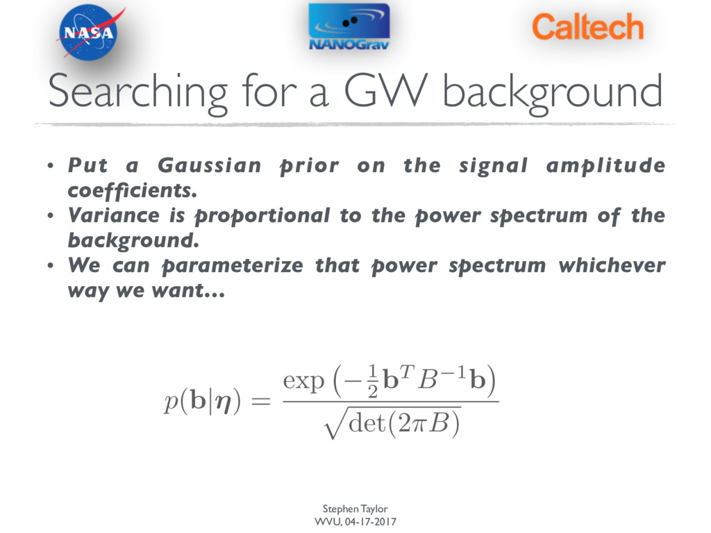
Put a Gaussian prior on the signal amplitude coefficients. • Variance is proportional to the power spectrum of the background. • We can parameterize that power spectrum whichever way we want…
( b|⌘ ) = exp 1 2 bT B 1b p det(2 ⇡B ) • Put a Gaussian prior on the signal amplitude coefficients. • Variance is proportional to the power spectrum of the background. • We can parameterize that power spectrum whichever way we want…
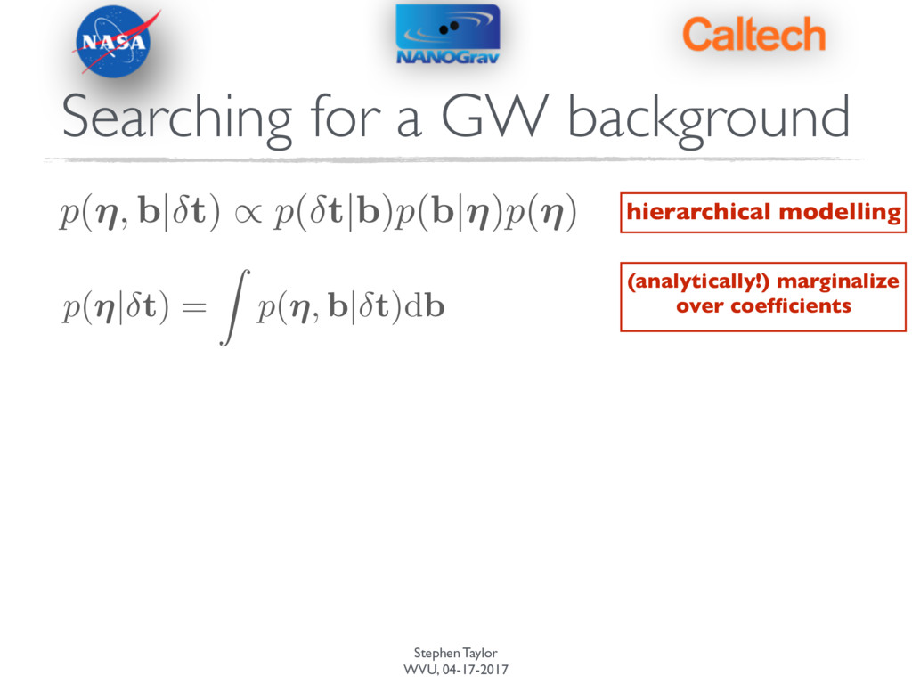
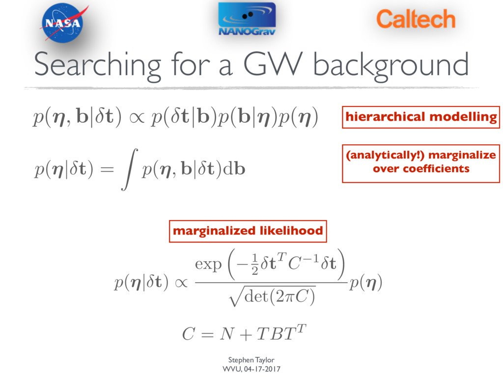
t)db p(⌘, b| t) / p( t|b)p(b|⌘)p(⌘) p ( ⌘| t ) / exp ⇣ 1 2 tT C 1 t ⌘ p det(2 ⇡C ) p ( ⌘ ) C = N + TBTT hierarchical modelling (analytically!) marginalize over coefficients marginalized likelihood Searching for a GW background
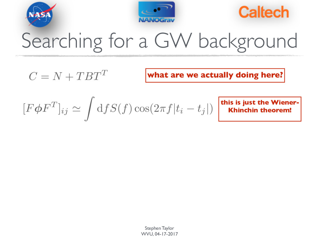
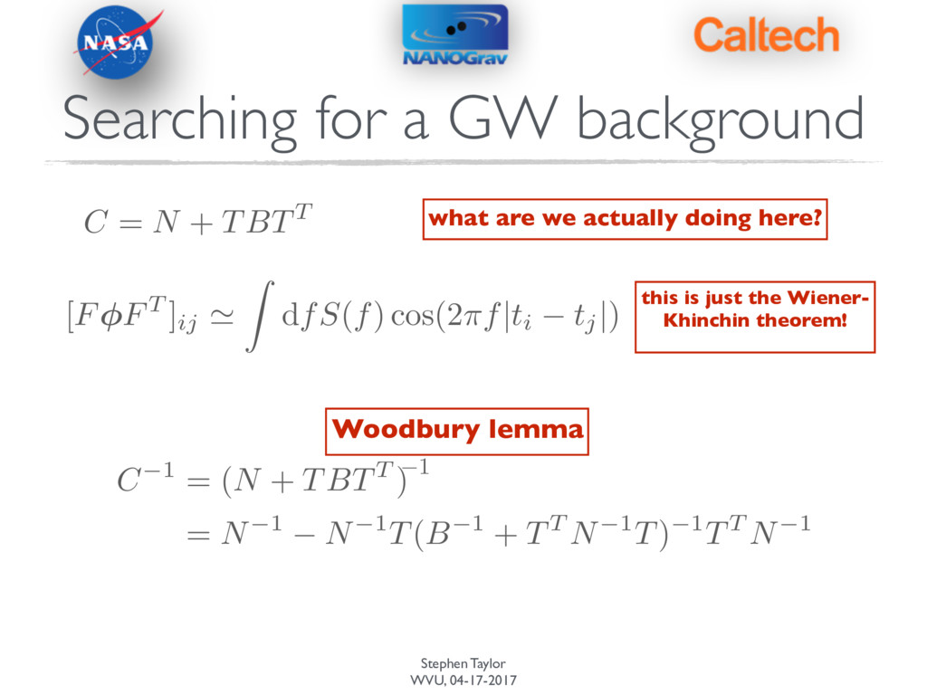
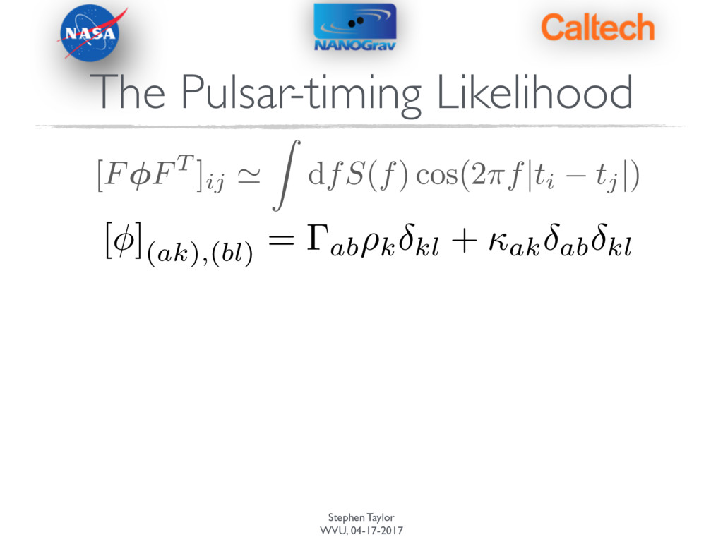
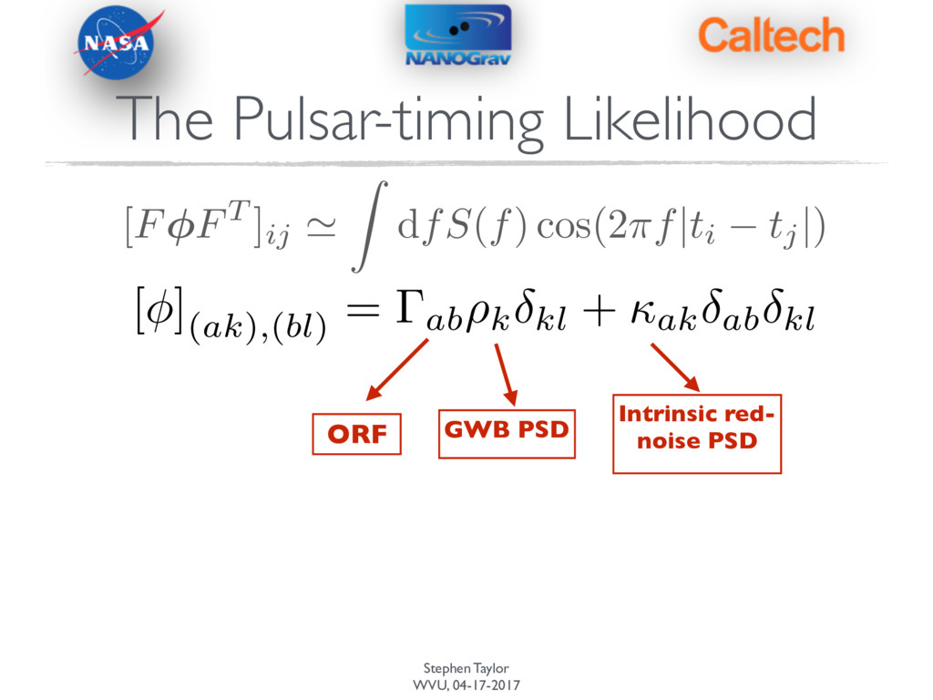
are we actually doing here? this is just the Wiener- Khinchin theorem! [ F FT ]ij ' Z d fS ( f ) cos(2 ⇡f|ti tj | ) C 1 = (N + TBTT ) = N 1 N 1T(B 1 + TT N 1T) 1TT N 1 Woodbury lemma 1 Searching for a GW background
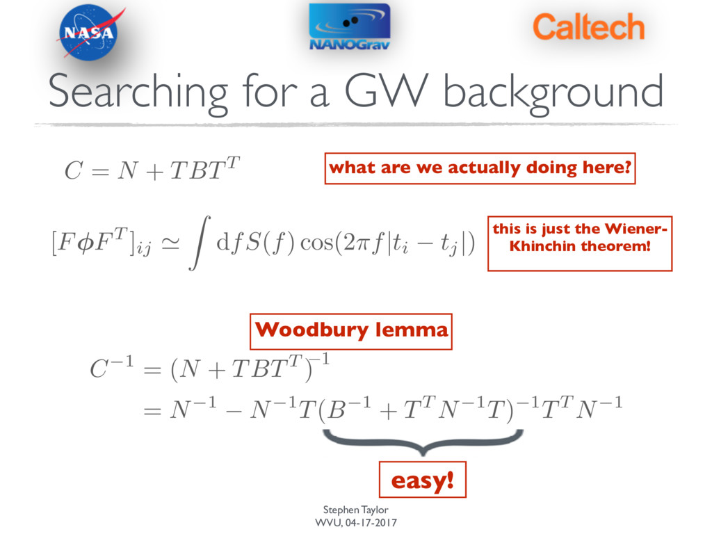
are we actually doing here? this is just the Wiener- Khinchin theorem! [ F FT ]ij ' Z d fS ( f ) cos(2 ⇡f|ti tj | ) C 1 = (N + TBTT ) = N 1 N 1T(B 1 + TT N 1T) 1TT N 1 easy! Woodbury lemma 1 Searching for a GW background
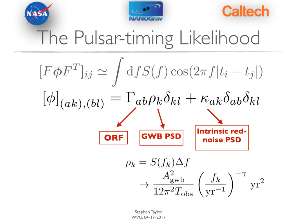
Intrinsic red- noise PSD [ F FT ]ij ' Z d fS ( f ) cos(2 ⇡f|ti tj | ) ⇢k = S(fk) f ! A2 gwb 12⇡2 T obs ✓ fk yr 1 ◆ yr2 [ ](ak),(bl) = ab⇢k kl + ak ab kl
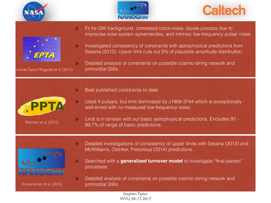
dipole process due to imprecise solar-system ephemerides, and intrinsic low-frequency pulsar noise. Investigated consistency of constraints with astrophysical predictions from Sesana (2013). Upper limit cuts out 5% of plausible amplitude distribution. Detailed analysis of constraints on possible cosmic-string network and primordial GWs Detailed investigations of consistency of upper limits with Sesana (2013) and McWilliams, Ostriker, Pretorious (2014) predictions. Searched with a generalized turnover model to investigate “final-parsec” processes. Detailed analysis of constraints on possible cosmic-string network and primordial GWs Best published constraints to date. Used 4 pulsars, but limit dominated by J1909-3744 which is exceptionally well-timed with no measured low-frequency noise. Limit is in tension with our basic astrophysical predictions. Excludes 91 - 99.7% of range of basic predictions. Lentati, Taylor, Mingarelli et al. (2015) Arzoumanian et al. (2016) Shannon et al. (2015)
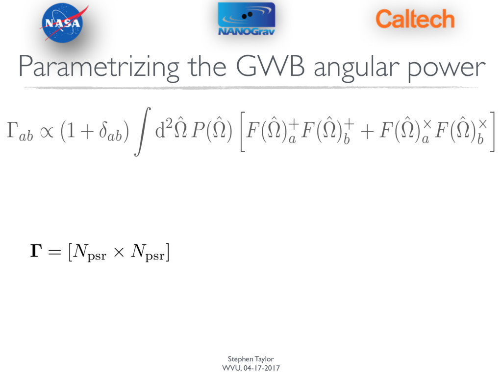
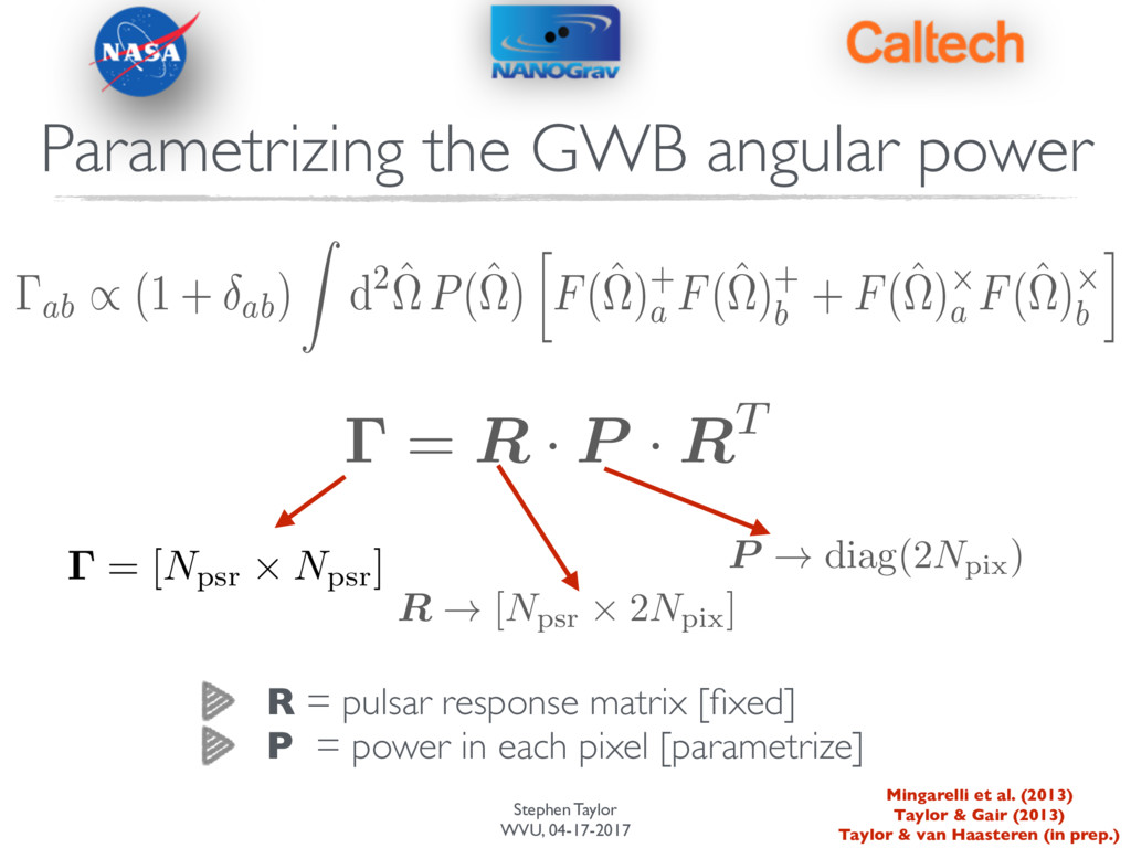
/ (1 + ab) Z d2 ˆ ⌦P(ˆ ⌦) h F(ˆ ⌦)+ a F(ˆ ⌦)+ b + F(ˆ ⌦)⇥ a F(ˆ ⌦)⇥ b i = R · P · RT R ! [N psr ⇥ 2N pix ] P ! diag(2N pix ) R = pulsar response matrix [fixed] P = power in each pixel [parametrize] Mingarelli et al. (2013) Taylor & Gair (2013) Taylor & van Haasteren (in prep.) = [Npsr ⇥ Npsr]
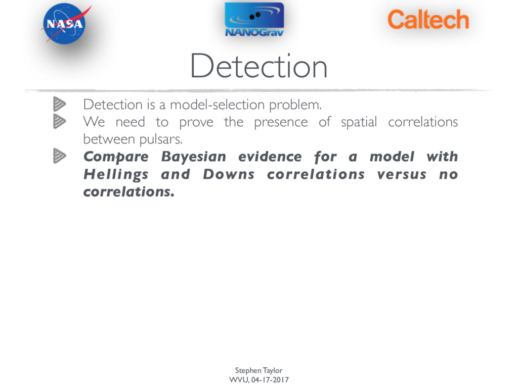
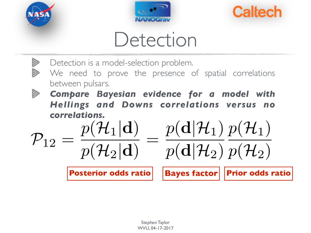
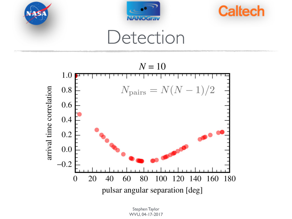
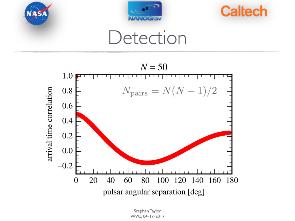
We need to prove the presence of spatial correlations between pulsars. Compare Bayesian evidence for a model with Hellings and Downs correlations versus no correlations.
We need to prove the presence of spatial correlations between pulsars. Compare Bayesian evidence for a model with Hellings and Downs correlations versus no correlations. P12 = p(H1 |d) p(H2 |d) = p(d|H1) p(d|H2) p(H1) p(H2) Posterior odds ratio Bayes factor Prior odds ratio
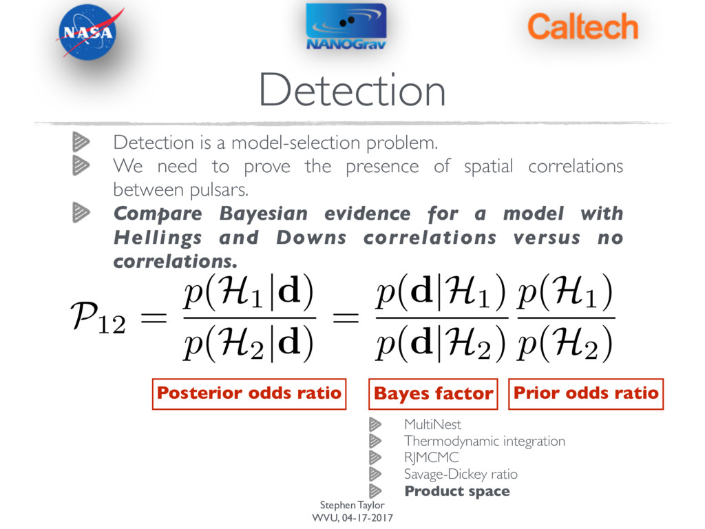
We need to prove the presence of spatial correlations between pulsars. Compare Bayesian evidence for a model with Hellings and Downs correlations versus no correlations. P12 = p(H1 |d) p(H2 |d) = p(d|H1) p(d|H2) p(H1) p(H2) Posterior odds ratio Bayes factor Prior odds ratio MultiNest Thermodynamic integration RJMCMC Savage-Dickey ratio Product space
area for statistical inference. We can do single-source searches and stochastic background searches all together in our pipelines. Current limits are cutting into astrophysically interesting territory. We can probe the dynamics and environments of supermassive black-holes binaries. Detection within 10 years (or even sooner) looks good.
tempo2.git) to read in “par” and “tim” files and to perform the timing-model analysis. Libstempo (https://github.com/vallis/libstempo) is a python module that wraps around TEMPO2. All our Bayesian codes interact with TEMPO2 using libstempo. Our production level codes include PAL2 (https:// github.com/jellis18/PAL2), NX01 (https://github.com/ stevertaylor/NX01), and Piccard (not in active development), and soon ENTERPRISE (https:// github.com/nanograv/enterprise).