Recovery Guarantees for Low Complexity Models

GT Image, IMB, Bordeaux, October 2013.

Transcript

1. Recovery Guarantees for Low Complexity Models Samuel Vaiter CEREMADE, Univ. Paris-Dauphine October 17, 2013 Séminaire Image, IMB, Bordeaux I
2. People & Papers • V., M. Golbabaee, M. J. Fadili et G. Peyré, Model Selection with Piecewise Regular Gauges, Tech. report, http://arxiv.org/abs/1307.2342 , 2013 • J. Fadili, V. and G. Peyré, Linear Convergence Rates for Gauge Regularization, ongoing work
3. Our work • Study of models, not algorithms • Impact of the noise • Understand the geometry 3 parts of this talk 1. Defining our framework of interest 2. Noise robustness results 3. Some examples
4. Linear Inverse Problem denoising inpainting deblurring
5. Linear Inverse Problem : Forward Model y = Φ x0 + w y ∈ RQ observations Φ ∈ RQ×N linear operator x0 ∈ RN unknown vector w ∈ RQ realization of a noise (bounded here)
6. Linear Inverse Problem : Forward Model y = Φ x0 + w y ∈ RQ observations Φ ∈ RQ×N linear operator x0 ∈ RN unknown vector w ∈ RQ realization of a noise (bounded here) Objective: Recover x0 from y.
7. The Variational Approach x ∈ argmin x∈RN F(y, x) + λ J(x) (Pλ(y)) Trade-off between data fidelity and prior regularization
8. The Variational Approach x ∈ argmin x∈RN F(y, x) + λ J(x) (Pλ(y)) Trade-off between data fidelity and prior regularization • Data fidelity: 2 loss, logistic, etc. F(y, x) = 1 2 ||y − Φx||2 2
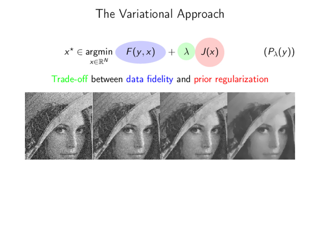
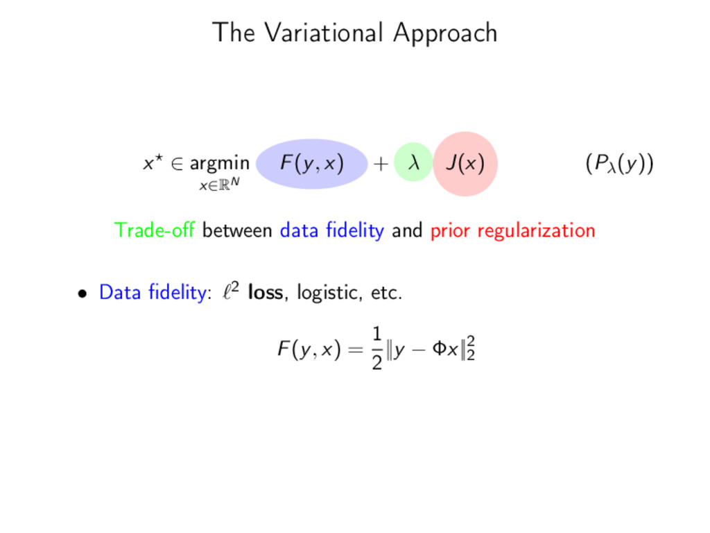
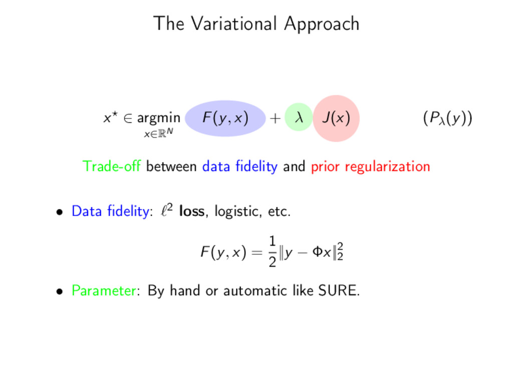
9. The Variational Approach x ∈ argmin x∈RN F(y, x) + λ J(x) (Pλ(y)) Trade-off between data fidelity and prior regularization • Data fidelity: 2 loss, logistic, etc. F(y, x) = 1 2 ||y − Φx||2 2 • Parameter: By hand or automatic like SURE.
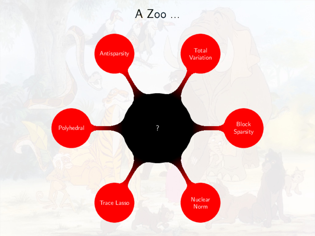
10. The Variational Approach x ∈ argmin x∈RN F(y, x) + λ J(x) (Pλ(y)) Trade-off between data fidelity and prior regularization • Data fidelity: 2 loss, logistic, etc. F(y, x) = 1 2 ||y − Φx||2 2 • Parameter: By hand or automatic like SURE. • Regularization: ?
11. A Zoo ... ? Block Sparsity Nuclear Norm Trace Lasso Polyhedral Antisparsity Total Variation
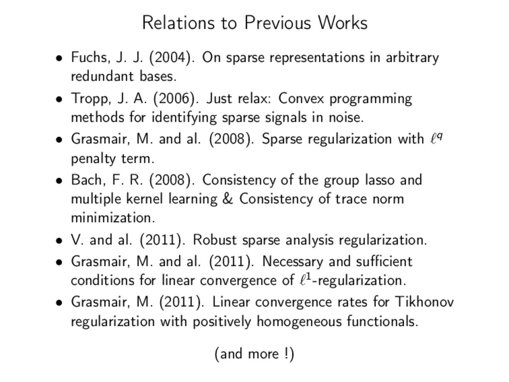
12. Relations to Previous Works • Fuchs, J. J. (2004). On sparse representations in arbitrary redundant bases. • Tropp, J. A. (2006). Just relax: Convex programming methods for identifying sparse signals in noise. • Grasmair, M. and al. (2008). Sparse regularization with q penalty term. • Bach, F. R. (2008). Consistency of the group lasso and multiple kernel learning & Consistency of trace norm minimization. • V. and al. (2011). Robust sparse analysis regularization. • Grasmair, M. and al. (2011). Necessary and sufficient conditions for linear convergence of 1-regularization. • Grasmair, M. (2011). Linear convergence rates for Tikhonov regularization with positively homogeneous functionals. (and more !)
13. First Part: Gauges and Model Space
14. Back to the Source: Union of Linear Models 2 components signal
15. Back to the Source: Union of Linear Models 2 components signal T0 0 is the only 0-sparse vector
16. Back to the Source: Union of Linear Models 2 components signal Te1 Te2 Axis points are 1-sparse (except 0)
17. Back to the Source: Union of Linear Models 2 components signal The whole space points minus the axis are 2-sparse
18. 0 to 1 Combinatorial penalty associated to the previous union of model J(x) = ||x||0 = | {i : xi = 0} |
19. 0 to 1 Combinatorial penalty associated to the previous union of model J(x) = ||x||0 = | {i : xi = 0} | → non-convex → no regularity → NP-hard regularization Encode Union of Model in a good functional
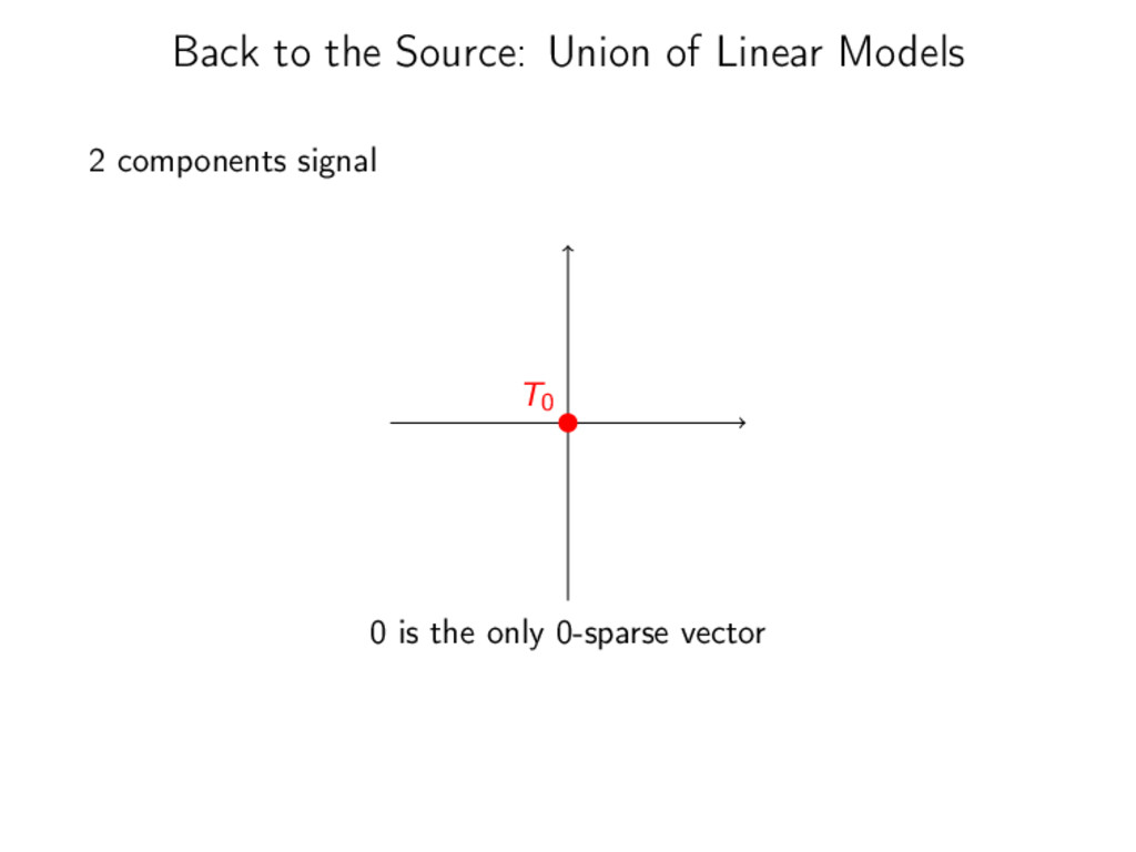
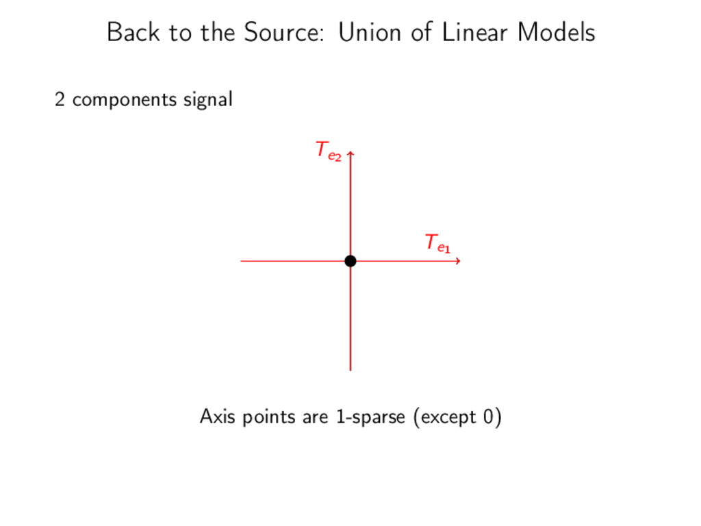
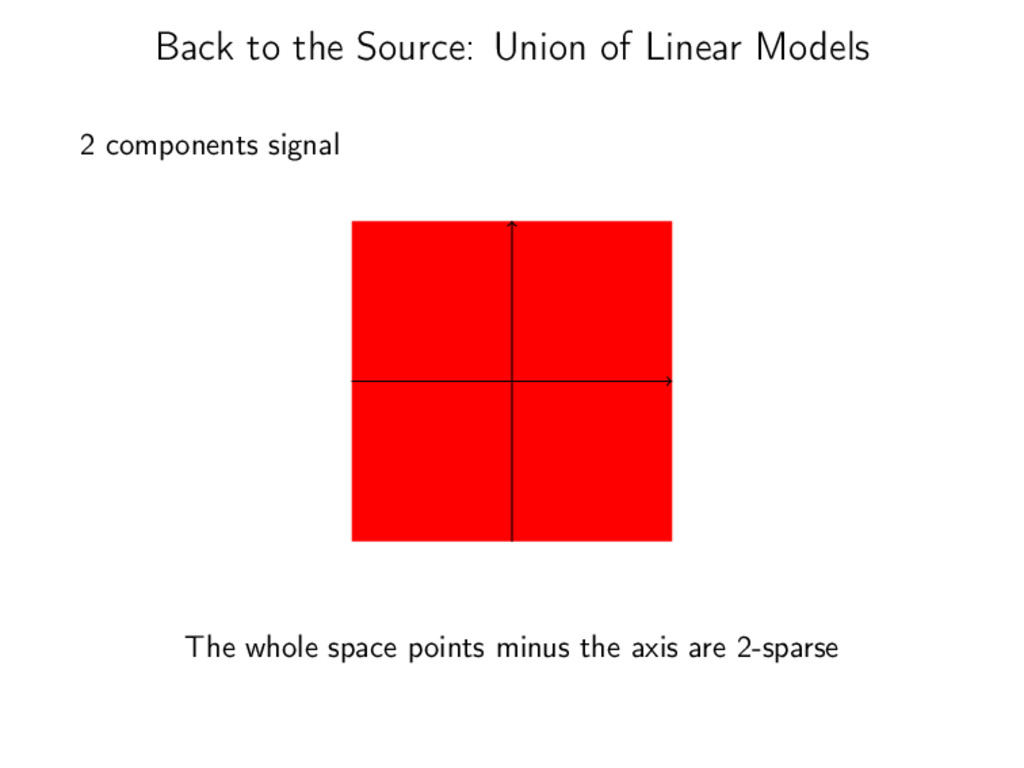
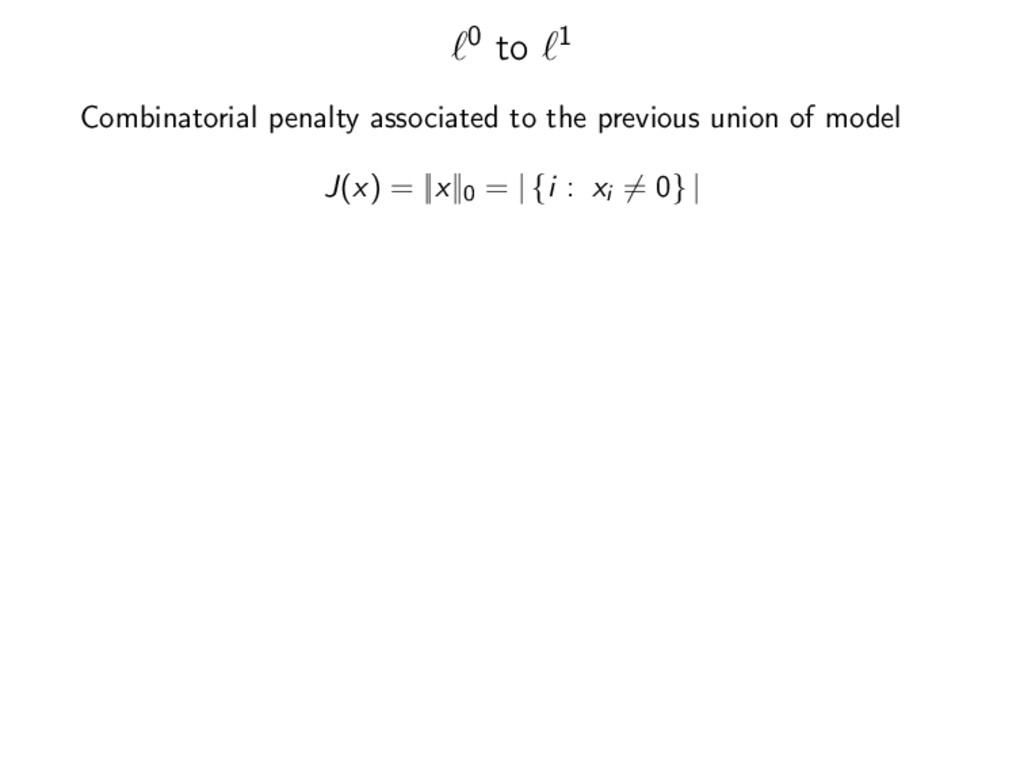
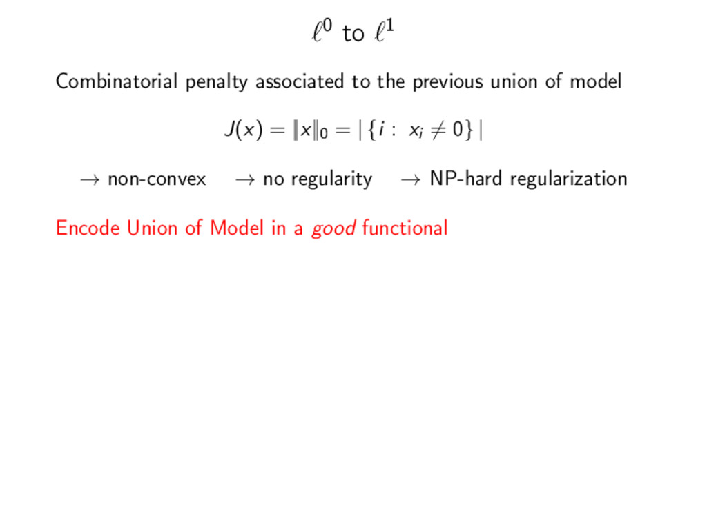
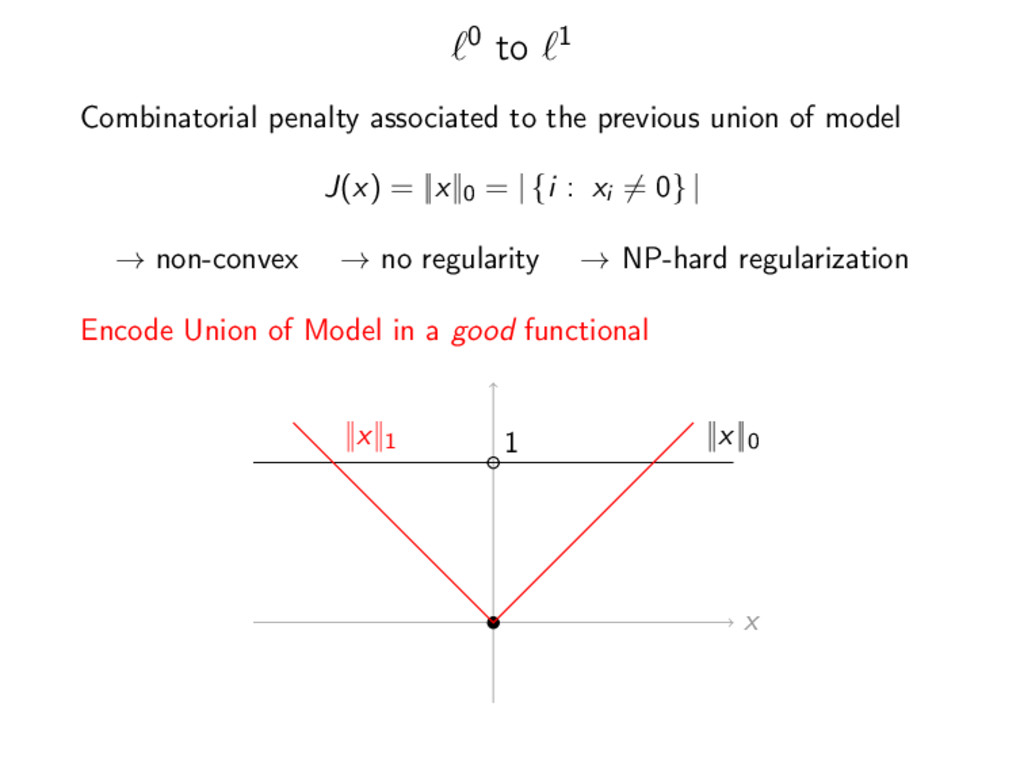
20. 0 to 1 Combinatorial penalty associated to the previous union of model J(x) = ||x||0 = | {i : xi = 0} | → non-convex → no regularity → NP-hard regularization Encode Union of Model in a good functional x ||x||0 1 ||x||1
21. Union of Linear Models to Regularizations Union of Model Gauges Combinatorial world Functional world
22. Gauge J(x) 0 J(λx) = λJ(x) for λ 0 J convex x → J(x) 1 C = {x : J(x) 1} C a convex set
23. Gauge J(x) 0 J(λx) = λJ(x) for λ 0 J convex x → J(x) 1 C = {x : J(x) 1} C a convex set
24. Subdifferential t f (t) (t, t2)
25. Subdifferential t f (t) (t, t2)
26. Subdifferential t f (t)
27. Subdifferential t f (t) ∂f (t) = η : f (t ) f (t) + η, t − t
28. The Model Linear Space 0 x
29. The Model Linear Space 0 x ∂J(x)
30. The Model Linear Space 0 x ∂J(x)
31. The Model Linear Space 0 x ∂J(x) Tx Tx = VectHull(∂J(x))⊥
32. The Model Linear Space 0 x ∂J(x) Tx ex Tx = VectHull(∂J(x))⊥ ex = PTx (∂J(x))
33. Special cases Sparsity Tx = {η : supp(η) ⊆ supp(x)} ex = sign(x)
34. Special cases Sparsity Tx = {η : supp(η) ⊆ supp(x)} ex = sign(x) (Aniso/Iso)tropic Total Variation Tx = {η : supp(∇η) ⊆ supp(∇x)} ex = sign(∇x) or ex = ∇x ||∇x||
35. Special cases Sparsity Tx = {η : supp(η) ⊆ supp(x)} ex = sign(x) (Aniso/Iso)tropic Total Variation Tx = {η : supp(∇η) ⊆ supp(∇x)} ex = sign(∇x) or ex = ∇x ||∇x|| Trace Norm SVD: x = UΛV ∗ Tx = {η : U∗ ⊥ ηV⊥ = 0} ex = UV ∗
36. Algebraic Stability Composition by a linear operator • ||∇ · ||1 — Anisotropic TV • ||∇ · ||1,2 — Istotropic TV • ||Udiag(·)||∗ — Trace Lasso
37. Algebraic Stability Composition by a linear operator • ||∇ · ||1 — Anisotropic TV • ||∇ · ||1,2 — Istotropic TV • ||Udiag(·)||∗ — Trace Lasso Sum of gauges (Composite priors) • || · ||1 + || · ||1 — sparse TV • || · ||1 + || · ||2 — Elastic net • || · ||1 + || · ||∗ — Sparse + Low-rank
38. Second Part: 2 Robustness and Model Selection
39. Certificate x ∈ argmin Φx=Φx0 J(x) (P0(y)) x Φx = Φx0
40. Certificate x ∈ argmin Φx=Φx0 J(x) (P0(y)) ∂J(x) x Φx = Φx0 η Dual certificates: D = Im Φ∗ ∩ ∂J(x0)
41. Certificate x ∈ argmin Φx=Φx0 J(x) (P0(y)) ∂J(x) x Φx = Φx0 η Dual certificates: D = Im Φ∗ ∩ ∂J(x0) Proposition ∃η ∈ D ⇔ x0 solution de (P0(y))
42. Tight Certificate and Restricted Injectivity Tight dual certificates ¯ D = Im Φ∗ ∩ ri ∂J(x)
43. Tight Certificate and Restricted Injectivity Tight dual certificates ¯ D = Im Φ∗ ∩ ri ∂J(x) Restricted Injectivity Ker Φ ∩ Tx = {0} (RICx )
44. Tight Certificate and Restricted Injectivity Tight dual certificates ¯ D = Im Φ∗ ∩ ri ∂J(x) Restricted Injectivity Ker Φ ∩ Tx = {0} (RICx ) Proposition ∃η ∈ ¯ D ∧ (RICx ) ⇒ x unique solution of (Pλ(y))
45. 2 stability Theorem If ∃η ∈ ¯ D ∧ (RICx ), then λ ∼ ||w|| ⇒ ||x − x || = O(||w||)
46. Minimal-norm Certificate η ∈ D ⇐⇒ η = Φ∗q, ηT = e and J◦(η) 1
47. Minimal-norm Certificate η ∈ D ⇐⇒ η = Φ∗q, ηT = e and J◦(η) 1 Minimal-norm precertificate η0 = argmin η=Φ∗q ηT =e ||q||
48. Minimal-norm Certificate η ∈ D ⇐⇒ η = Φ∗q, ηT = e and J◦(η) 1 Minimal-norm precertificate η0 = argmin η=Φ∗q ηT =e ||q|| Proposition If (RICx ), then η0 = (Φ+ T Φ)∗e
49. Model Selection Theorem If η0 ∈ ¯ D, the noise-to-signal ratio is low enough and λ ∼ ||w||, the unique solution x of (Pλ(y)) satifies Tx = Tx0 and ||x − x || = O(||w||)
50. A Better Certificate ? • With model selection: no
51. A Better Certificate ? • With model selection: no • Without: ongoing works Duval-Peyré: Sparse Deconvolution Dossal: Sparse Tomography
52. Third Part: Some Examples
53. Sparse Spike Deconvolution (Dossal, 2005) x0
54. Sparse Spike Deconvolution (Dossal, 2005) Φx = i xi ϕ(· − ∆i) J(x) = ||x||1 x0 γ Φx0
55. Sparse Spike Deconvolution (Dossal, 2005) Φx = i xi ϕ(· − ∆i) J(x) = ||x||1 x0 γ Φx0 η0 ∈ ¯ D ⇔ ||Φ+,∗ Ic ΦI s||∞ < 1 γ ||η0,Ic ||∞ γcrit 1
56. TV Denoising (V. et al., 2011) Φ = Id J(x) = ||∇x||1 i xi i xi
57. TV Denoising (V. et al., 2011) Φ = Id J(x) = ||∇x||1 i xi i xi k mk k mk +1 −1
58. TV Denoising (V. et al., 2011) Φ = Id J(x) = ||∇x||1 i xi i xi k mk k mk +1 −1 Support stability No support stability
59. TV Denoising (V. et al., 2011) Φ = Id J(x) = ||∇x||1 i xi i xi k mk k mk +1 −1 Support stability No support stability Both are 2-stable
60. Thanks for your attention !