Golden-cheeked Warbler Habitat Change: Gains and Losses Through Time

Nancy Heger - Texas Parks and Wildlife Department | Tom Hayes - Environmental Conservation Alliance

Transcript

1. Trends in Golden-cheeked Warbler Habitat Change Through Time By Nancy A. Heger and Tom Hayes NAH: Texas Parks and Wildlife TH: Environmental Conservation Alliance, Inc.
2. Agenda Ø  Overview •  Background •  Problem Ø  “Previously at the TNRIS GIS Forum” •  Summary of previous work via web app Ø  Analysis of past decade (2004-05 to 2016) •  Review of methodology and problems •  Results •  On-going web app dev •  Web App Ø  Conclusions
3. Golden-cheeked Warblers (GCWA) Setophaga chrysoparia (Dendroica chrysoparia) Ø  Prominent golden-cheeks Ø  Females & juveniles less showy than males Ø  Nest only in Central Texas; Texas Hill Country (THC) Ø  Winter in Mexico and Central America Male Female
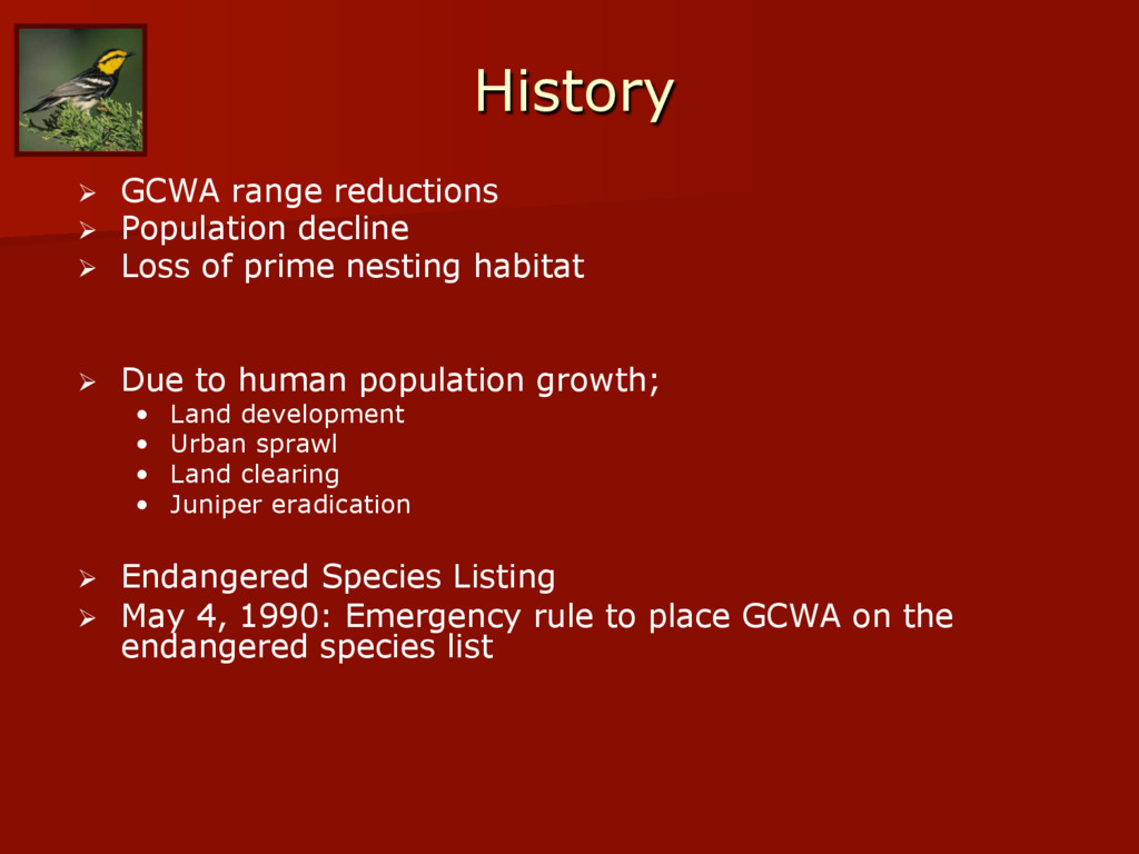
4. History Ø  GCWA range reductions Ø  Population decline Ø  Loss of prime nesting habitat Ø  Due to human population growth; •  Land development •  Urban sprawl •  Land clearing •  Juniper eradication Ø  Endangered Species Listing Ø  May 4, 1990: Emergency rule to place GCWA on the endangered species list
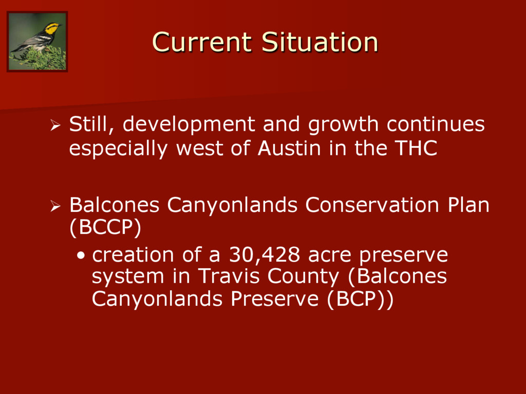
5. Current Situation Ø  Still, development and growth continues especially west of Austin in the THC Ø  Balcones Canyonlands Conservation Plan (BCCP) • creation of a 30,428 acre preserve system in Travis County (Balcones Canyonlands Preserve (BCP))
6. Previous Assessments and current Objectives Ø  Previous Research: usually single time- point estimations of population numbers and available habitat Ø  But, to discern long term trends in loss or gain of habitat, need to use the same methodology across time Ø  Our objective: to use consistent methodology to discern long term trends in GCWA Habitat •  Both losses and gains
7. Ø  Apples to Apples: Conduct the assessment the same each time period so they are comparable. Ø  Same geospatial data type Ø  Use Similar Phenological cycle image (similar time within a season) Ø  Same Pixel Resolution (spatial resolution, 6in, 1ft, 1m, 10m, 30m) Ø  Same Spectral Resolution (true color, color infrared, multispectral) Thus, for a 30 year study, we were limited to the technology available in the mid 1980s; Satellite imagery Technological Prerequisites for Habitat Change Detection Objective: Objective:
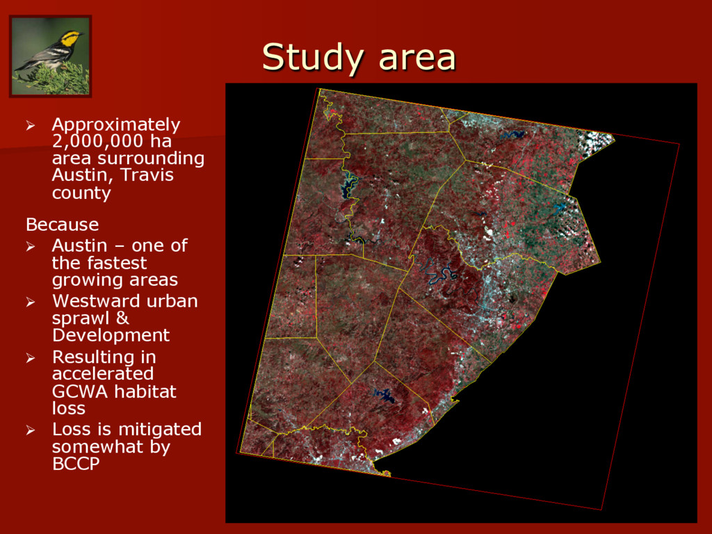
8. Study area Ø  Approximately 2,000,000 ha area surrounding Austin, Travis county Because Ø  Austin – one of the fastest growing areas Ø  Westward urban sprawl & Development Ø  Resulting in accelerated GCWA habitat loss Ø  Loss is mitigated somewhat by BCCP
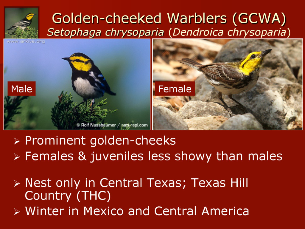
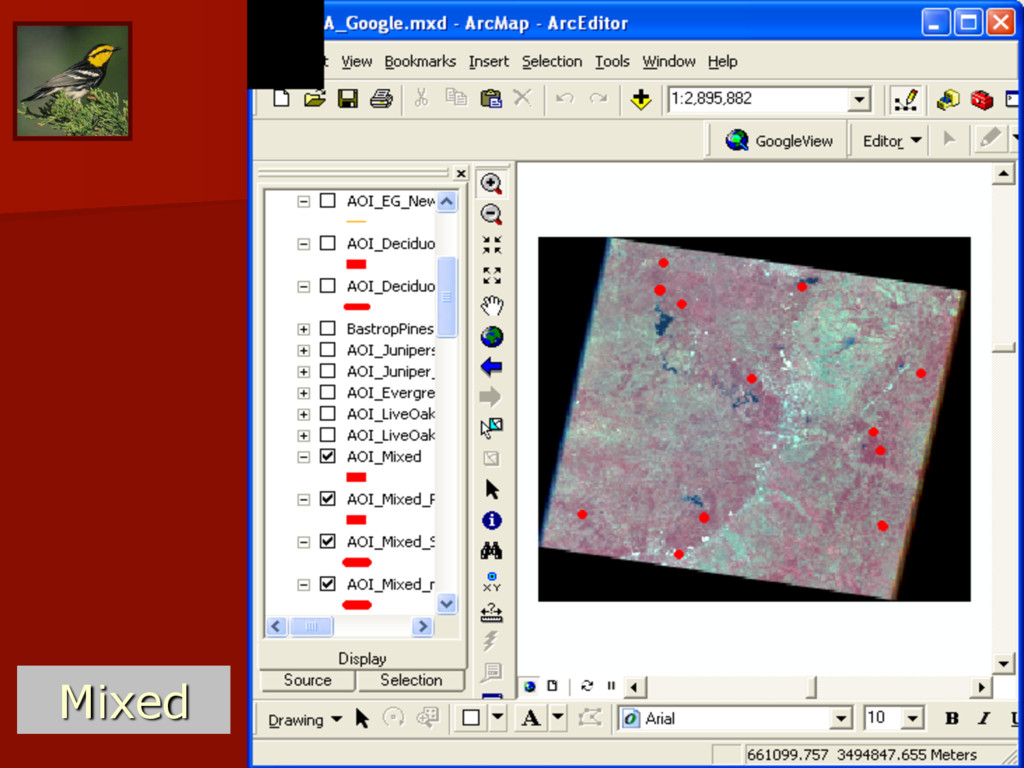
9. Modeling GCWA Habitat Ø  Typical Nesting Habitat: Ashe juniper-oak woodland (Mixed habitat) Ø  Only mature junipers (20-30 yrs; 4.5 m tall) produce shredding bark for nesting Prefers Ø  thick canopy Ø  dense forests Ø  large tracts Ø  >100m from edges
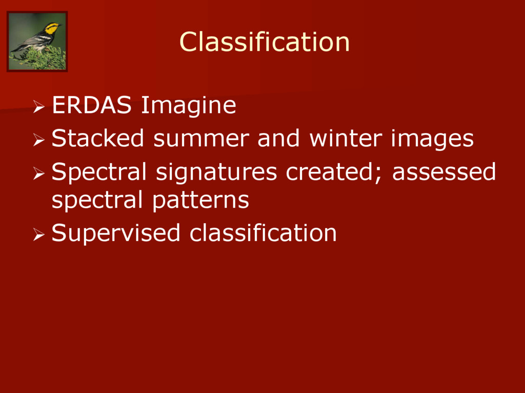
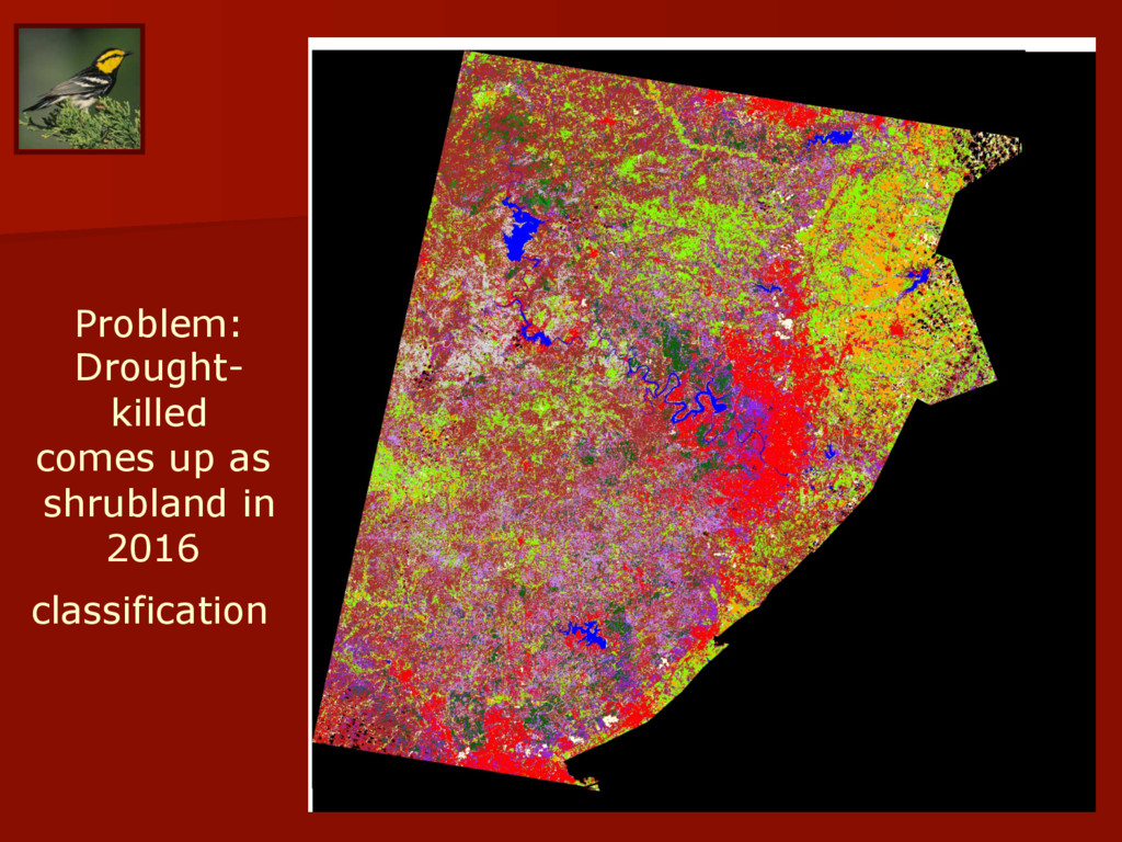
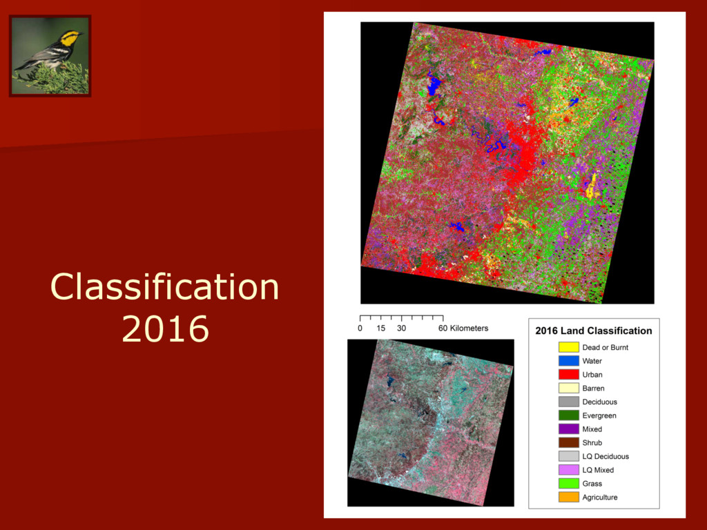
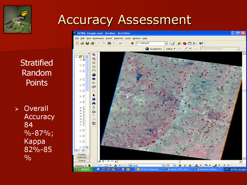
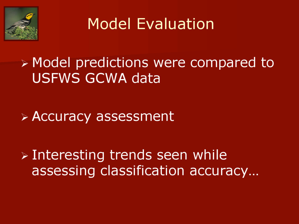
10. Methodology Ø  Select summer & winter satellite images Ø  Conduct supervised classifications of stacked images separately for each decade Ø  Conduct Accuracy analysis Ø  Identify gains and losses in GCWA habitat through time
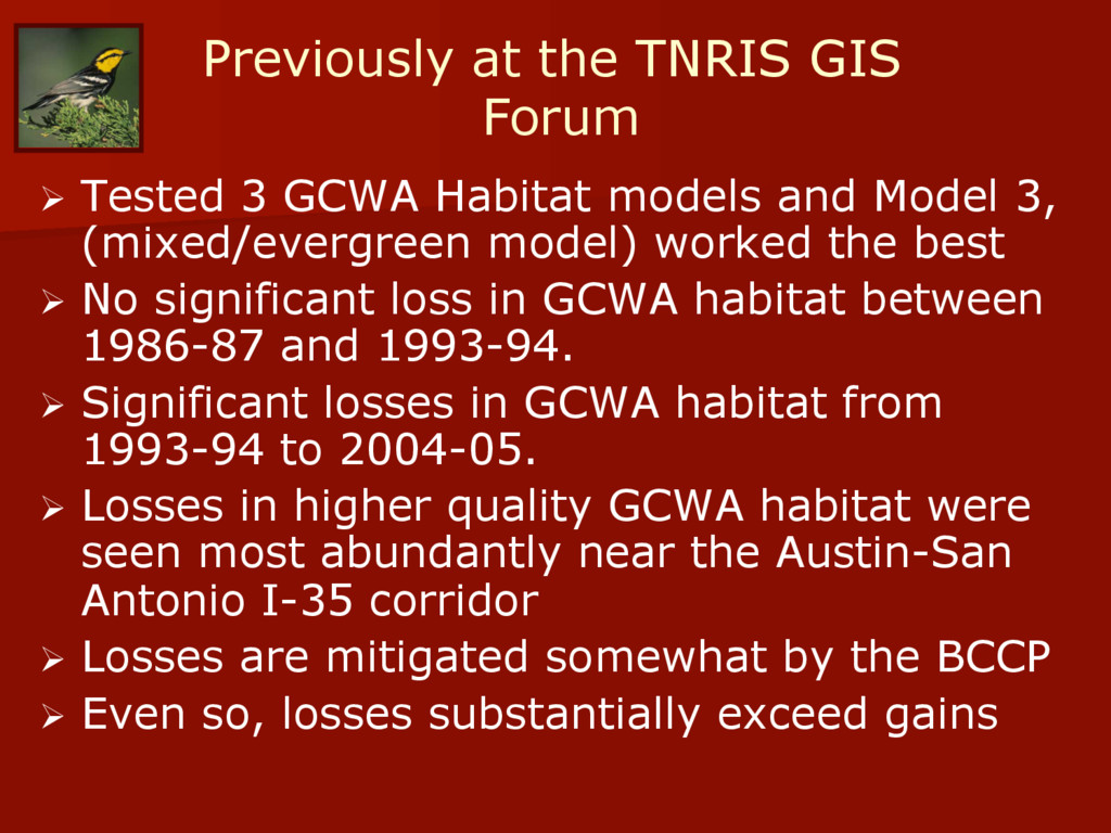
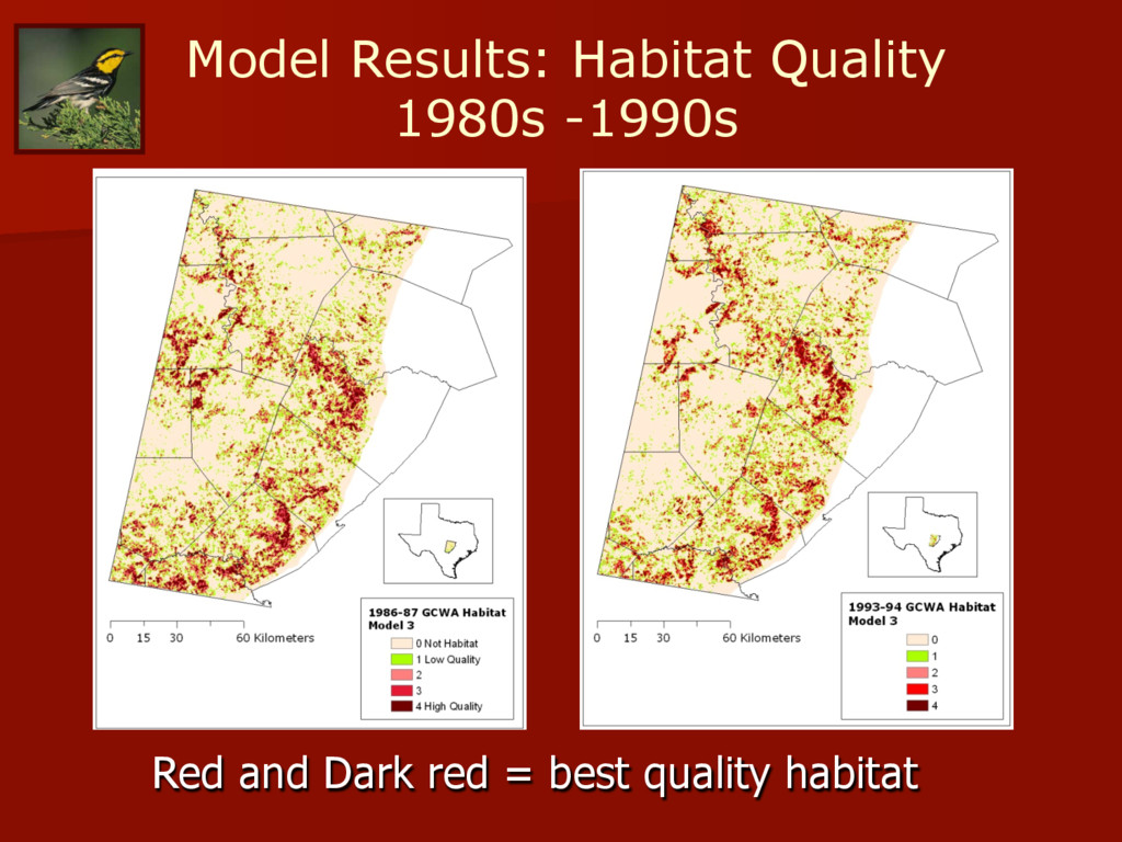
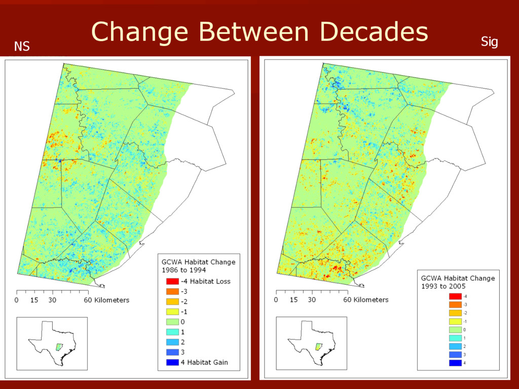
11. Previously at the TNRIS GIS Forum Ø  Tested 3 GCWA Habitat models and Model 3, (mixed/evergreen model) worked the best Ø  No significant loss in GCWA habitat between 1986-87 and 1993-94. Ø  Significant losses in GCWA habitat from 1993-94 to 2004-05. Ø  Losses in higher quality GCWA habitat were seen most abundantly near the Austin-San Antonio I-35 corridor Ø  Losses are mitigated somewhat by the BCCP Ø  Even so, losses substantially exceed gains
12. App. Demo
13. Continuation of study Ø One more decade: 2004-05 to 2016 Ø Major events since last time • Recession • Drought of 2011 • Landsat 5 and Landsat 8
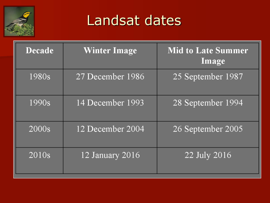
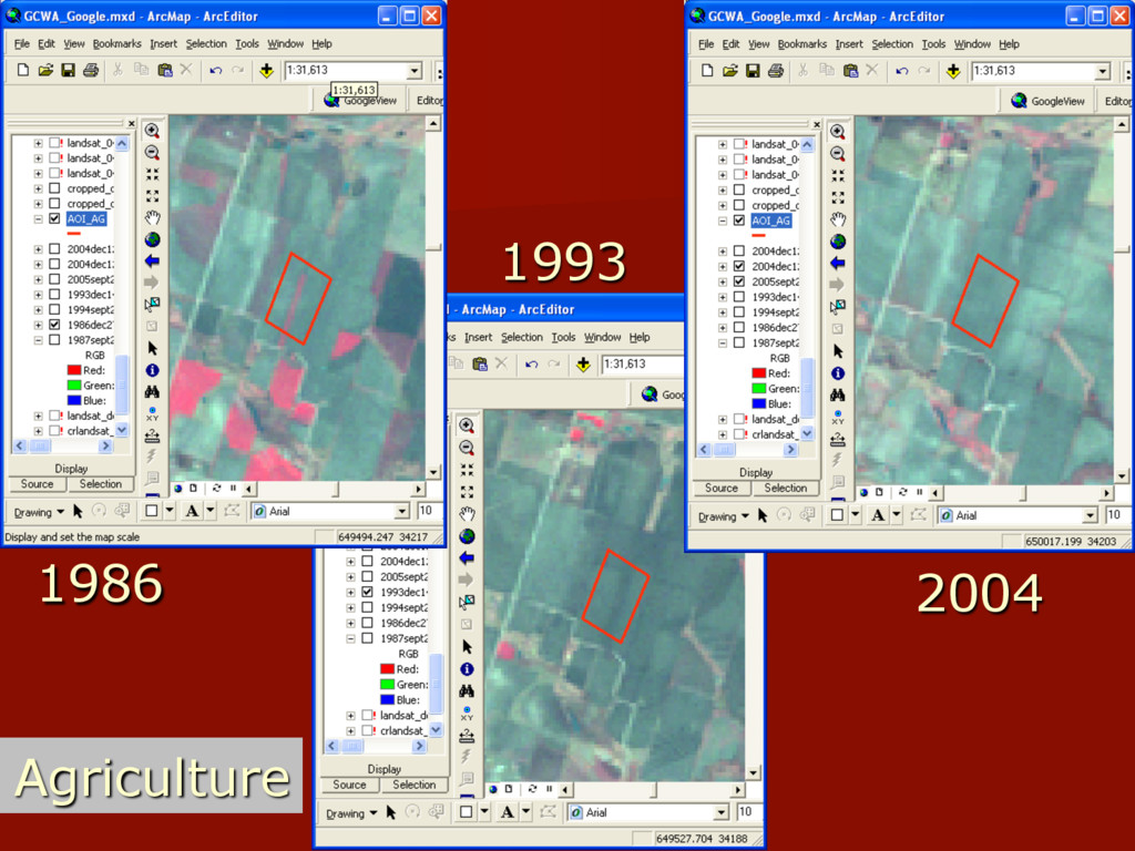
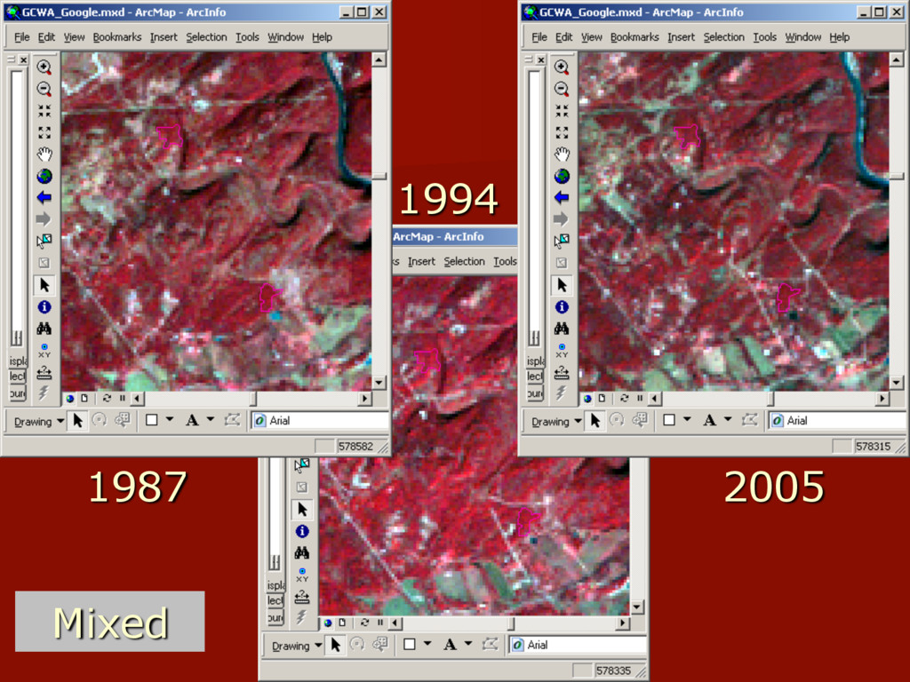
14. Landsat dates Decade Winter Image Mid to Late Summer Image 1980s 27 December 1986 25 September 1987 1990s 14 December 1993 28 September 1994 2000s 12 December 2004 26 September 2005 2010s 12 January 2016 22 July 2016
15. Methodology – Same as last time Ø  Select summer & winter satellite images Ø  Conduct supervised classifications of stacked images separately for each decade Ø  Conduct Accuracy analysis Ø  Identify gains and losses in GCWA habitat through time
16. Winter Summer Deciduous Forest
17. Land Classes Open Water Urban Barren Deciduous forest Evergreen forest Mixed Forest Shrubland Grassland Agriculture
18. Classification Ø ERDAS Imagine Ø Stacked summer and winter images Ø Spectral signatures created; assessed spectral patterns Ø Supervised classification
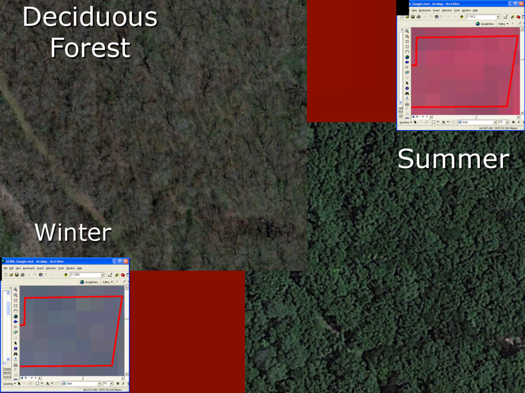
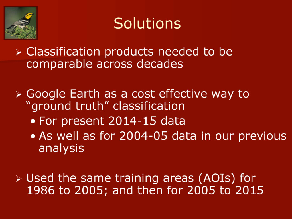
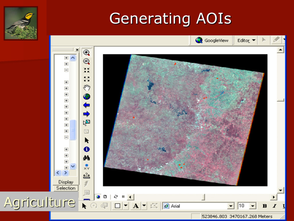
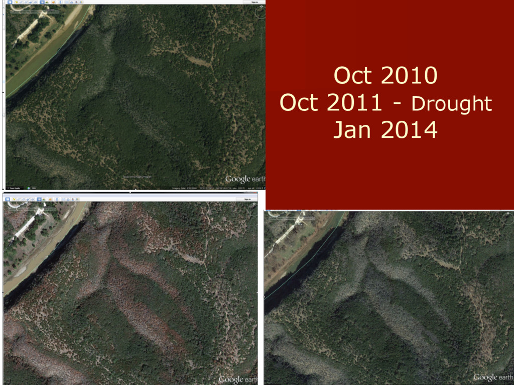
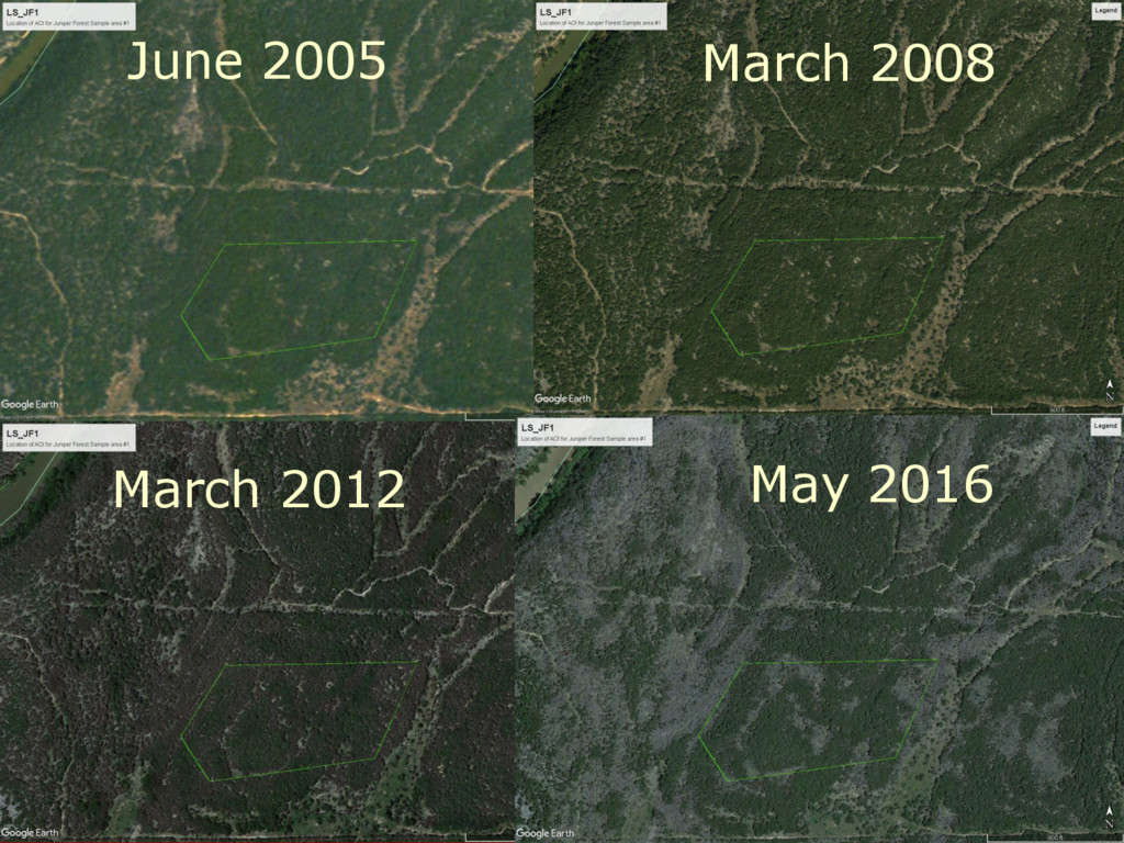
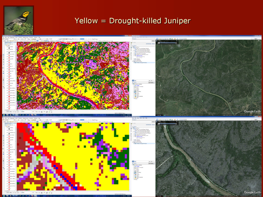
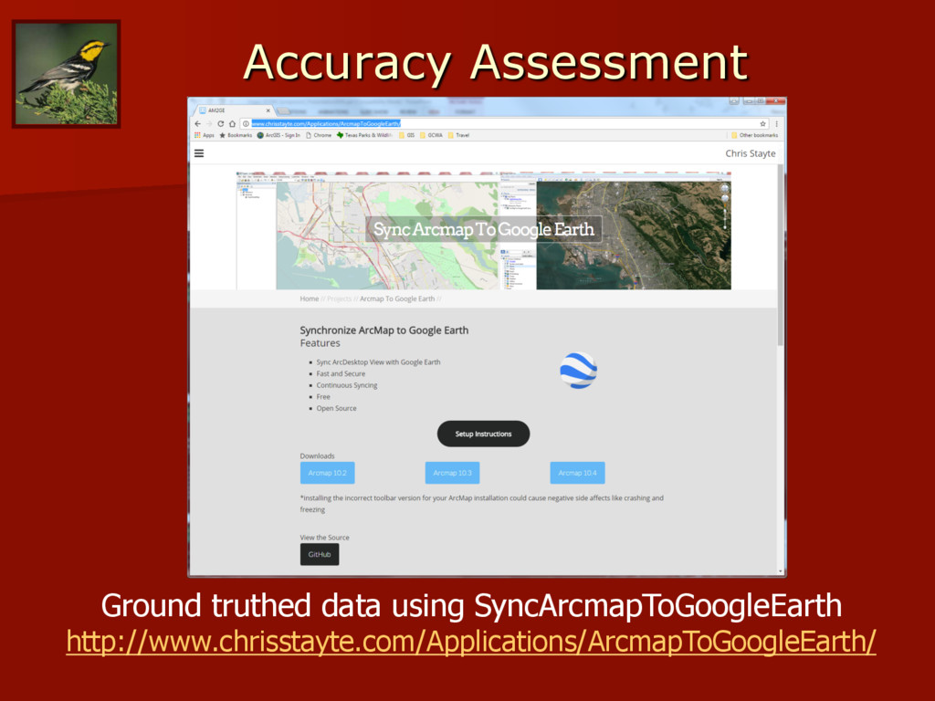
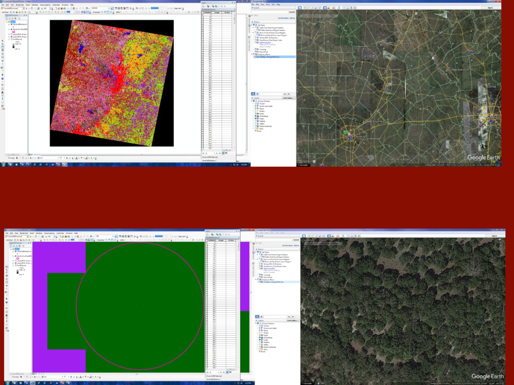
19. Solutions Ø  Classification products needed to be comparable across decades Ø  Google Earth as a cost effective way to “ground truth” classification • For present 2014-15 data • As well as for 2004-05 data in our previous analysis Ø  Used the same training areas (AOIs) for 1986 to 2005; and then for 2005 to 2015
20. Generating AOIs Agriculture
21. 1986 1993 2004 Agriculture
22. Mixed
23. 1987 Mixed 1994 2005
24. Classifications
25. Problem: Drought- killed comes up as shrubland in 2016 classification
26. Classification 2016
27. Oct 2010 Oct 2011 - Drought Jan 2014
28. March 2012 June 2005 May 2016 March 2008
29. Yellow = Drought-killed Juniper
30. Accuracy Assessment Stratified Random Points Ø  Overall Accuracy 84 %-87%; Kappa 82%-85 %
31. Accuracy Assessment Ground truthed data using SyncArcmapToGoogleEarth http://www.chrisstayte.com/Applications/ArcmapToGoogleEarth/
32. Accuracy Assessment
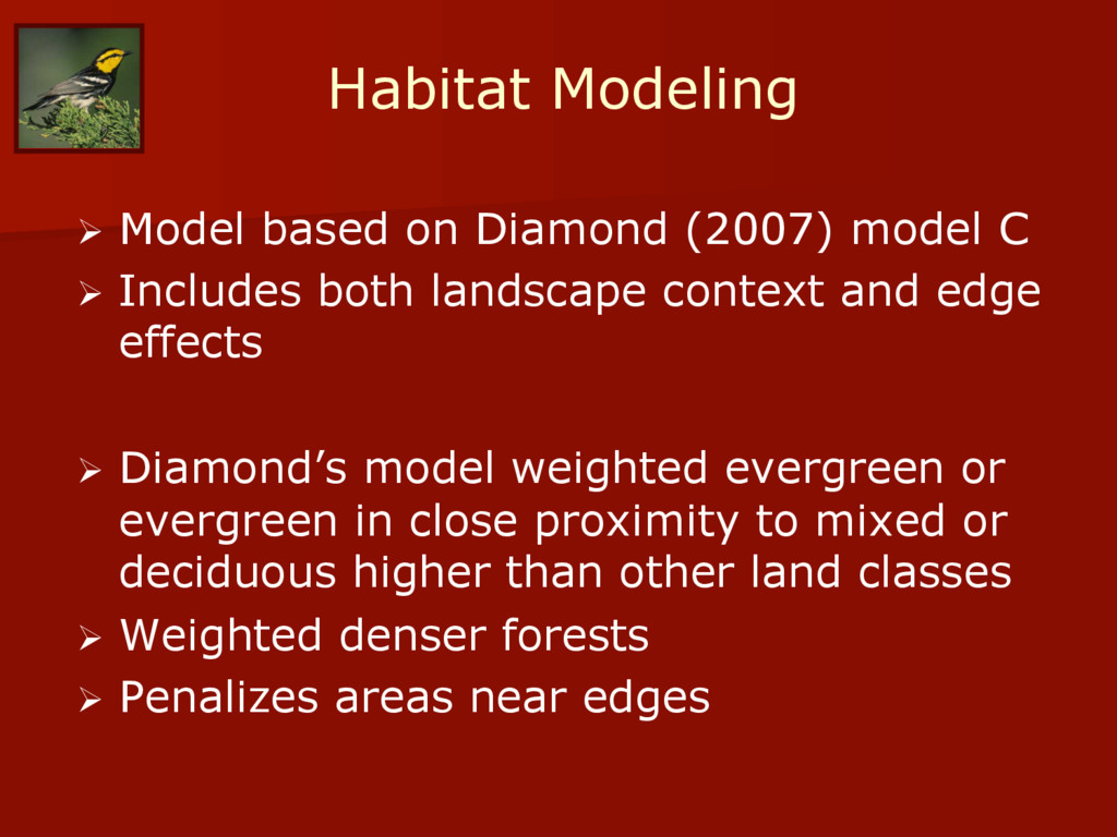
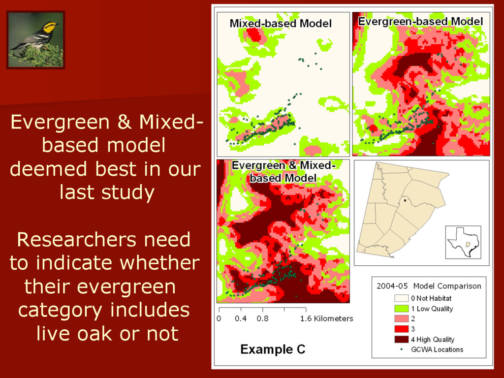
33. Habitat Modeling Ø  Model based on Diamond (2007) model C Ø  Includes both landscape context and edge effects Ø  Diamond’s model weighted evergreen or evergreen in close proximity to mixed or deciduous higher than other land classes Ø  Weighted denser forests Ø  Penalizes areas near edges
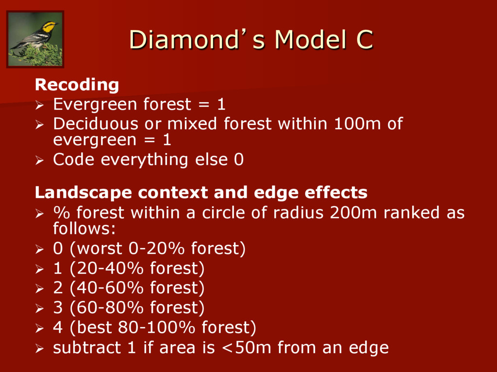
34. Diamond’s Model C Recoding Ø  Evergreen forest = 1 Ø  Deciduous or mixed forest within 100m of evergreen = 1 Ø  Code everything else 0 Landscape context and edge effects Ø  % forest within a circle of radius 200m ranked as follows: Ø  0 (worst 0-20% forest) Ø  1 (20-40% forest) Ø  2 (40-60% forest) Ø  3 (60-80% forest) Ø  4 (best 80-100% forest) Ø  subtract 1 if area is <50m from an edge
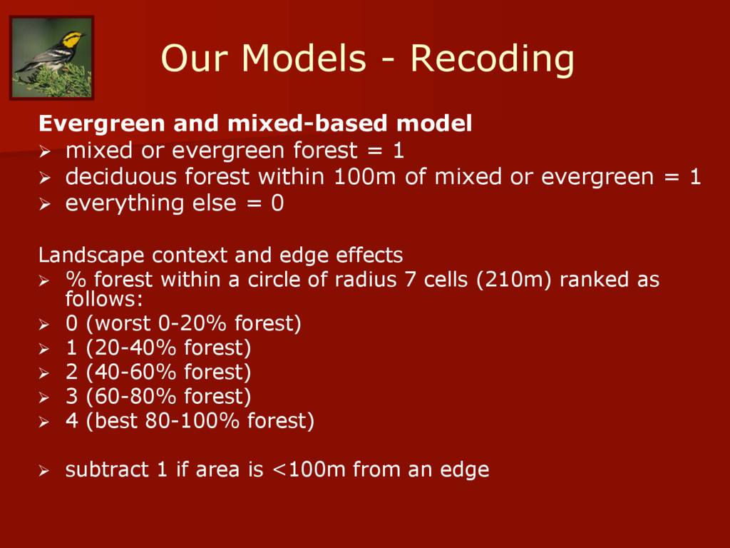
35. Our Models - Recoding Evergreen and mixed-based model Ø  mixed or evergreen forest = 1 Ø  deciduous forest within 100m of mixed or evergreen = 1 Ø  everything else = 0 Landscape context and edge effects Ø  % forest within a circle of radius 7 cells (210m) ranked as follows: Ø  0 (worst 0-20% forest) Ø  1 (20-40% forest) Ø  2 (40-60% forest) Ø  3 (60-80% forest) Ø  4 (best 80-100% forest) Ø  subtract 1 if area is <100m from an edge
37. Model Evaluation Ø Model predictions were compared to USFWS GCWA data Ø Accuracy assessment Ø Interesting trends seen while assessing classification accuracy…
38. Evergreen & Mixed- based model deemed best in our last study Researchers need to indicate whether their evergreen category includes live oak or not
39. Model Results: Habitat Quality 1980s -1990s Red and Dark red = best quality habitat
40. Model Results 2000s-2010s Red and Dark red = best quality habitat
41. Assessing Change 1.  Overall percent of each class 2.  Change between decades assessed by rank differences (-4 to +4) •  Positive indicates gains •  Negative indicates losses
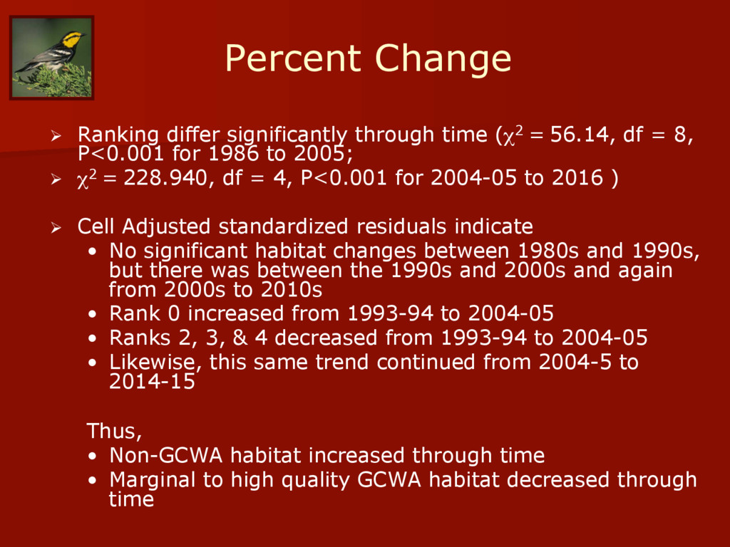
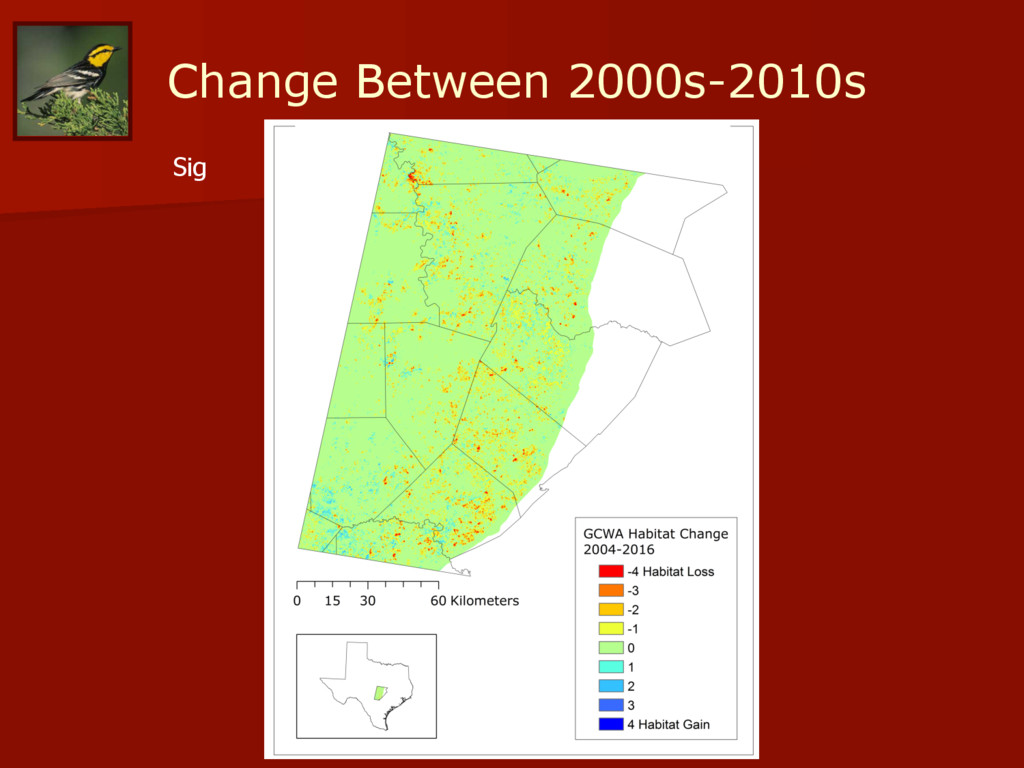
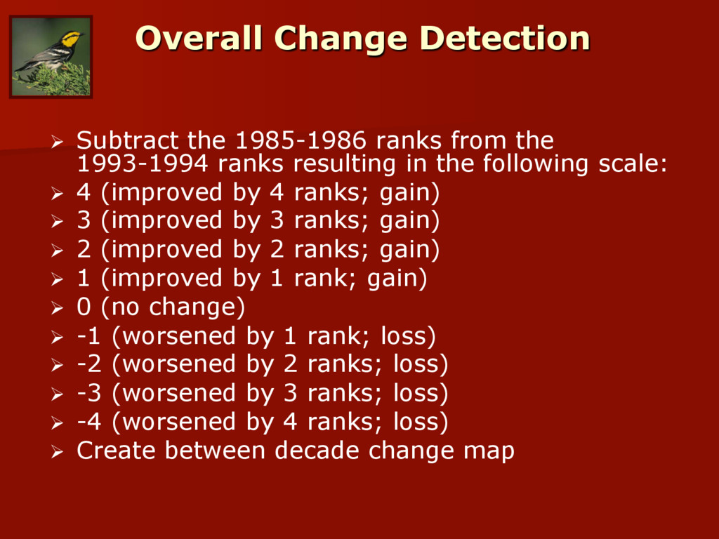
42. Percent Change Ø  Ranking differ significantly through time (χ2 = 56.14, df = 8, P<0.001 for 1986 to 2005; Ø  χ2 = 228.940, df = 4, P<0.001 for 2004-05 to 2016 ) Ø  Cell Adjusted standardized residuals indicate •  No significant habitat changes between 1980s and 1990s, but there was between the 1990s and 2000s and again from 2000s to 2010s •  Rank 0 increased from 1993-94 to 2004-05 •  Ranks 2, 3, & 4 decreased from 1993-94 to 2004-05 •  Likewise, this same trend continued from 2004-5 to 2014-15 Thus, •  Non-GCWA habitat increased through time •  Marginal to high quality GCWA habitat decreased through time
43. Change Between Decades NS Sig
44. Change Between 2000s-2010s Sig
45. Conclusions Ø  Losses in GCWA habitat have accelerated from 1993-94 to 2004-05 and also from 2004-5 to 2016 Ø  Losses in higher quality GCWA habitat are seen most abundantly near the Austin-San Antonio I-35 corridor Ø  Losses are mitigated somewhat by the BCCP Ø  Even so, losses substantially exceed gains
46. Significance Ø Information on gains and losses helps to • Access where to focus GCWA habitat restoration/preservation efforts • Access effectiveness of past management Ø Protecting GCWA also • Protects others species • Protects the Edwards aquifer
47. Photo Sources Ø  Title slide Male GCWA – USFWS Ø  Species slide Male GCWA - Rolf Nussbaumer, naturepl.com Ø  Female GCWA - texasgloria52 on flickr.com Ø  Oak-Juniper woodland – TPWD, GIS Lab Ø  Lost Maples, Oak-Juniper – scilogs.com
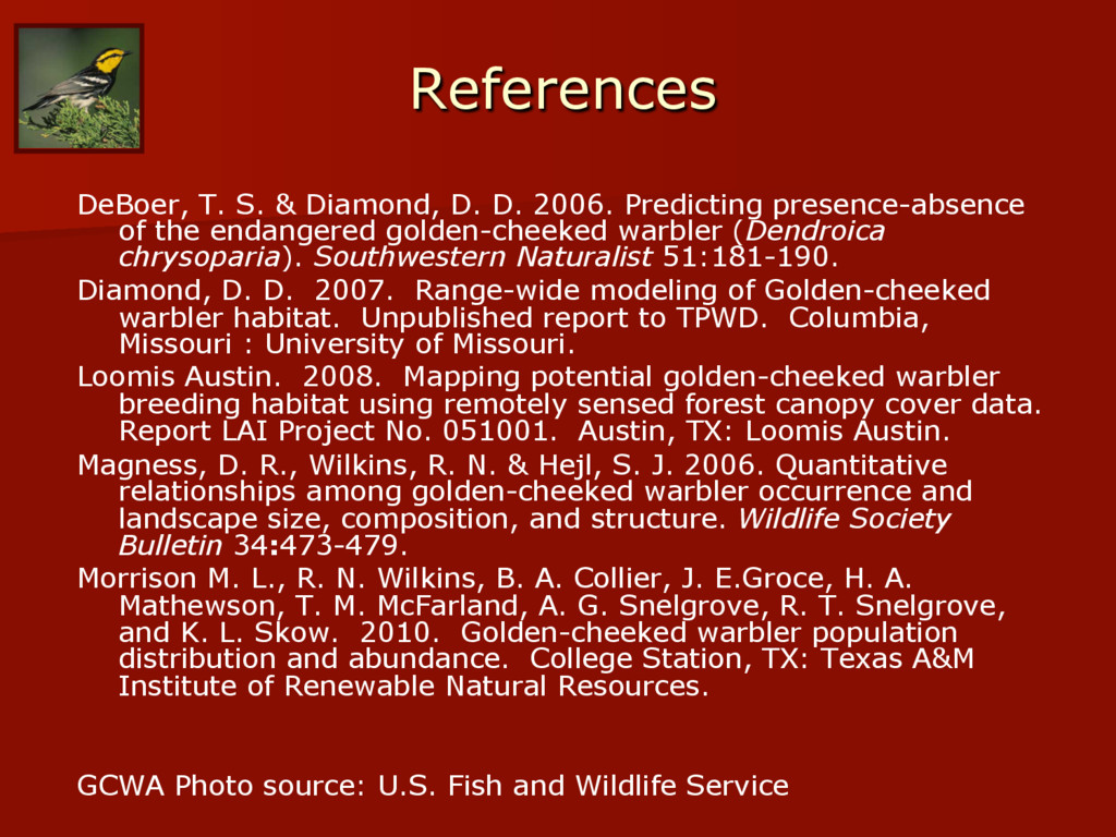
48. References DeBoer, T. S. & Diamond, D. D. 2006. Predicting presence-absence of the endangered golden-cheeked warbler (Dendroica chrysoparia). Southwestern Naturalist 51:181-190. Diamond, D. D. 2007. Range-wide modeling of Golden-cheeked warbler habitat. Unpublished report to TPWD. Columbia, Missouri : University of Missouri. Loomis Austin. 2008. Mapping potential golden-cheeked warbler breeding habitat using remotely sensed forest canopy cover data. Report LAI Project No. 051001. Austin, TX: Loomis Austin. Magness, D. R., Wilkins, R. N. & Hejl, S. J. 2006. Quantitative relationships among golden-cheeked warbler occurrence and landscape size, composition, and structure. Wildlife Society Bulletin 34:473-479. Morrison M. L., R. N. Wilkins, B. A. Collier, J. E.Groce, H. A. Mathewson, T. M. McFarland, A. G. Snelgrove, R. T. Snelgrove, and K. L. Skow. 2010. Golden-cheeked warbler population distribution and abundance. College Station, TX: Texas A&M Institute of Renewable Natural Resources. GCWA Photo source: U.S. Fish and Wildlife Service
49. Questions?
50. Overall Change Detection Ø  Subtract the 1985-1986 ranks from the 1993-1994 ranks resulting in the following scale: Ø  4 (improved by 4 ranks; gain) Ø  3 (improved by 3 ranks; gain) Ø  2 (improved by 2 ranks; gain) Ø  1 (improved by 1 rank; gain) Ø  0 (no change) Ø  -1 (worsened by 1 rank; loss) Ø  -2 (worsened by 2 ranks; loss) Ø  -3 (worsened by 3 ranks; loss) Ø  -4 (worsened by 4 ranks; loss) Ø  Create between decade change map