Towards a Model Selection Rule for Quantum State Tomography

How can we use model selection to make quantum state tomography better? I discuss how a commonly-used technique, loglikelihood ratios, run into problems because the state space has boundaries.

Transcript

1. Towards a Model Selection Rule for Quantum State Tomography Travis L Scholten @Travis_Sch Center for Quantum Information and Control, UNM Center for Computing Research, Sandia National Labs SQuInT Workshop 2016 February 19 Sandia National Laboratories is a multi-program laboratory managed and operated by Sandia Corporation, a wholly owned subsidiary of Lockheed Martin Corporation, for the U.S. Department of Energy’s National Nuclear Security Administration under contract DE-AC04-94AL85000. CCR Center for Computing Research
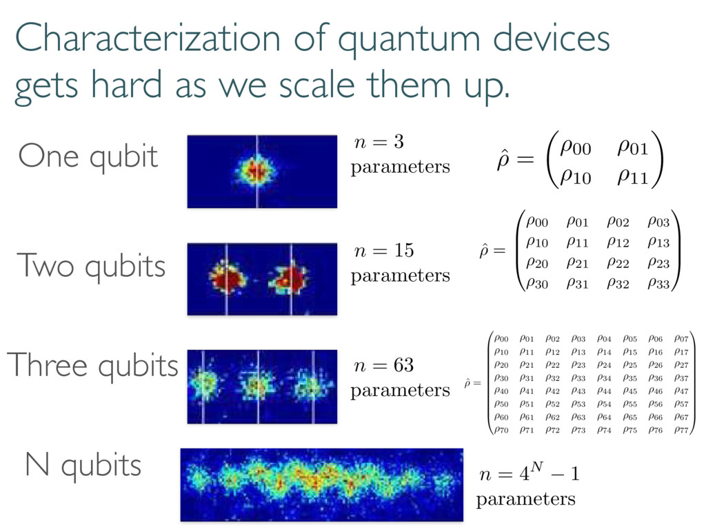
2. Characterization of quantum devices gets hard as we scale them up. One qubit Two qubits N qubits Three qubits ˆ ⇢ = ✓ ⇢00 ⇢01 ⇢10 ⇢11 ◆ ˆ ⇢ = 0 B B @ ⇢00 ⇢01 ⇢02 ⇢03 ⇢10 ⇢11 ⇢12 ⇢13 ⇢20 ⇢21 ⇢22 ⇢23 ⇢30 ⇢31 ⇢32 ⇢33 1 C C A ˆ ⇢ = 0 B B B B B B B B B B @ ⇢00 ⇢01 ⇢02 ⇢03 ⇢04 ⇢05 ⇢06 ⇢07 ⇢10 ⇢11 ⇢12 ⇢13 ⇢14 ⇢15 ⇢16 ⇢17 ⇢20 ⇢21 ⇢22 ⇢23 ⇢24 ⇢25 ⇢26 ⇢27 ⇢30 ⇢31 ⇢32 ⇢33 ⇢34 ⇢35 ⇢36 ⇢37 ⇢40 ⇢41 ⇢42 ⇢43 ⇢44 ⇢45 ⇢46 ⇢47 ⇢50 ⇢51 ⇢52 ⇢53 ⇢54 ⇢55 ⇢56 ⇢57 ⇢60 ⇢61 ⇢62 ⇢63 ⇢64 ⇢65 ⇢66 ⇢67 ⇢70 ⇢71 ⇢72 ⇢73 ⇢74 ⇢75 ⇢76 ⇢77 1 C C C C C C C C C C A n = 3 parameters n = 15 parameters n = 63 parameters n = 4N 1 parameters
3. Model selection can make tomography more tractable. Model (for tomography) = sets of density matrices Model selection = find best model What sets will we consider? What does best mean? ˆ ⇢ = 0 @ 1 A
4. Tomographers have been doing model selection all along. Model (for tomography) = sets of density matrices Trivial way: ˆ ⇢ = 0 @ 1 A Pick Hilbert space by fiat (“Of course it’s a qubit!”)
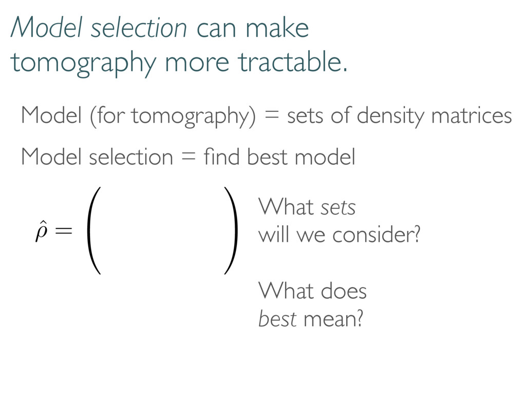
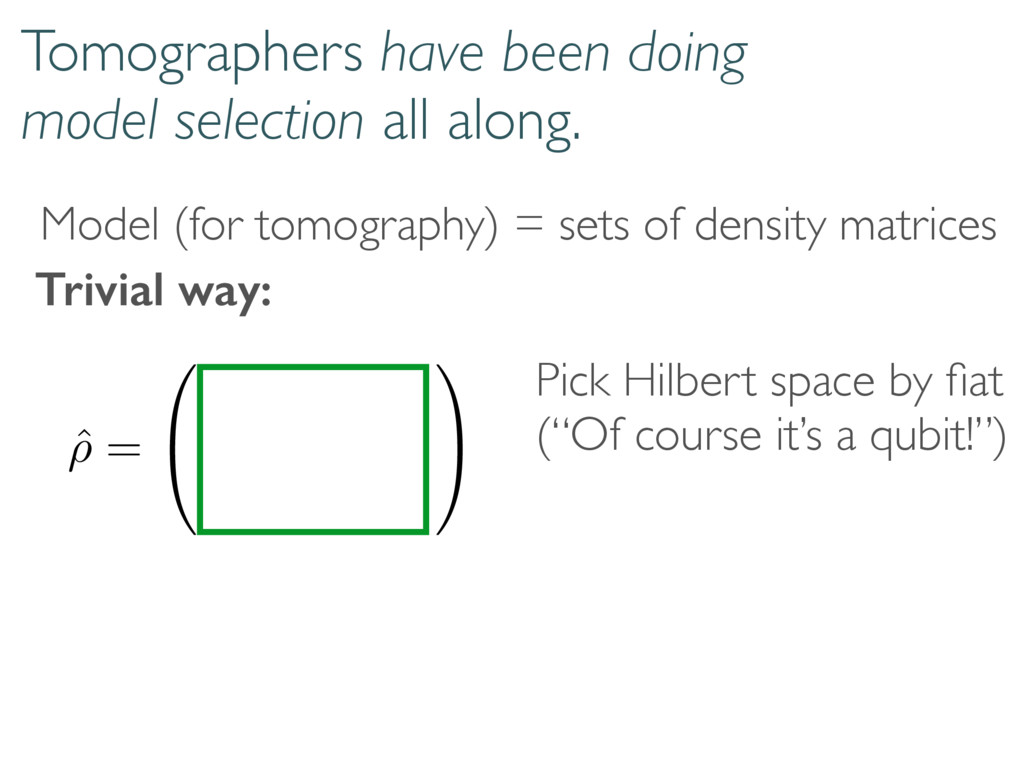
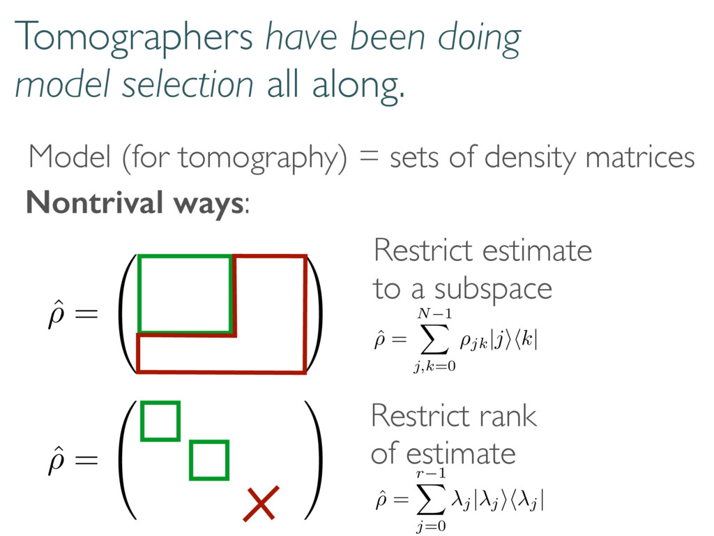
5. Tomographers have been doing model selection all along. Model (for tomography) = sets of density matrices ˆ ⇢ = 0 @ 1 A Restrict estimate to a subspace ˆ ⇢ = 0 @ 1 A Restrict rank of estimate ˆ ⇢ = N 1 X j,k=0 ⇢jk |jihk| ˆ ⇢ = r 1 X j=0 j | j ih j | Nontrival ways:
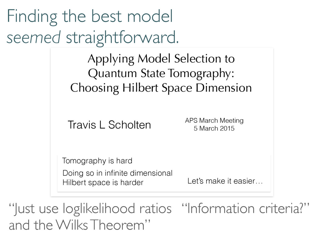
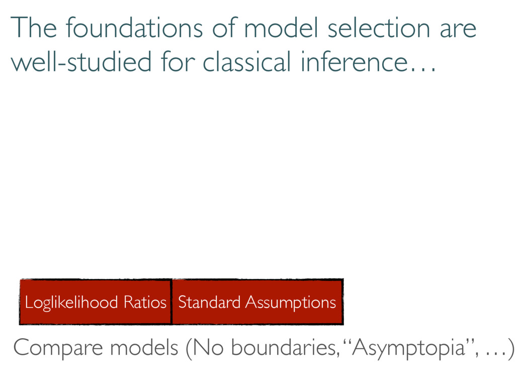
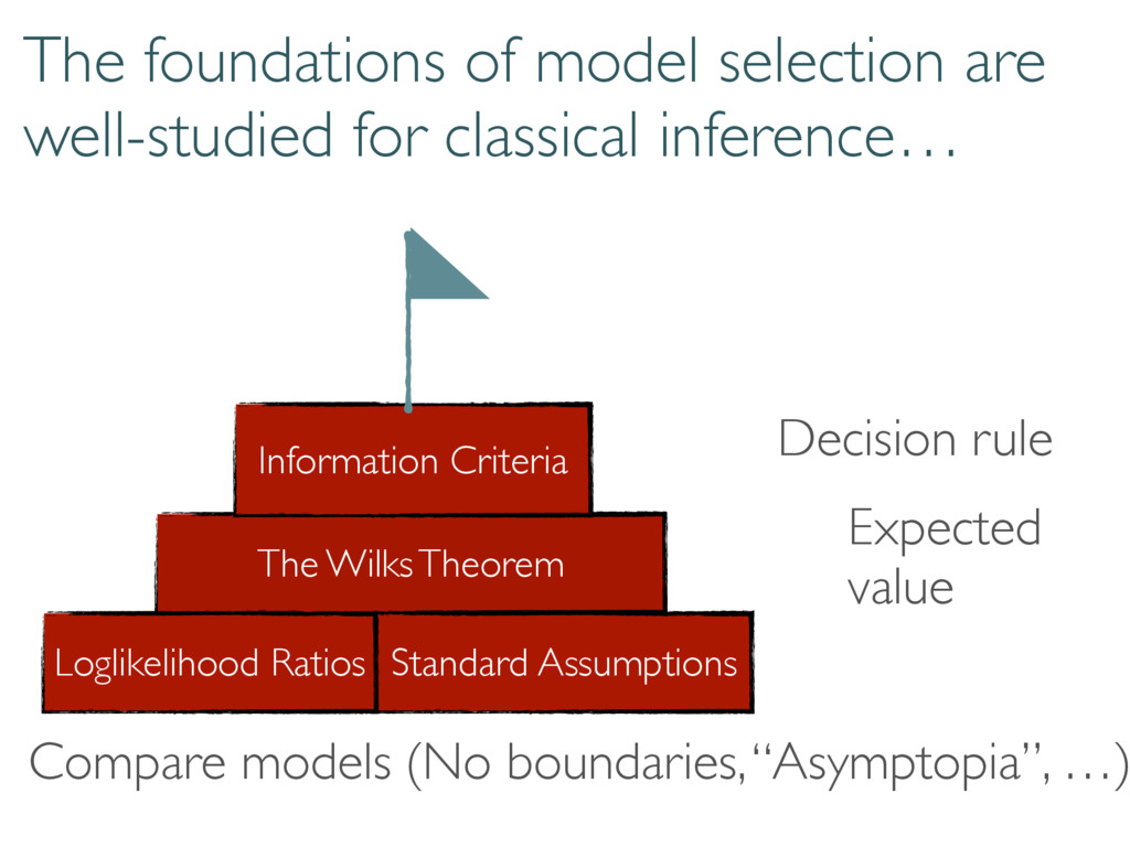
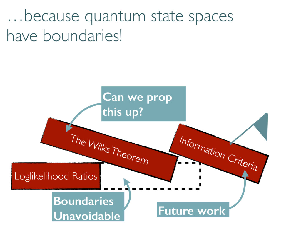
6. Applying Model Selection to Quantum State Tomography: Choosing Hilbert Space Dimension Travis L Scholten APS March Meeting 5 March 2015 Tomography is hard Sandia National Laboratories is a multi-program laboratory managed and operated by Sandia Corporation, a wholly owned subsidiary of Lockheed Martin Corporation, for the U.S. Department of Energy’s National Nuclear Security Administration under contract DE-AC04-94AL85000. Let’s make it easier… Doing so in infinite dimensional Hilbert space is harder Finding the best model seemed straightforward. “Just use loglikelihood ratios and the Wilks Theorem” “Information criteria?”
7. Wilks Theorem: predicts expected evidence when model contains truth Hmm…?! A key tool used for model selection — the Wilks Theorem — failed dramatically!
8. How did this happen?!
9. The foundations of model selection are well-studied for classical inference… Standard Assumptions (No boundaries, “Asymptopia”, …)
10. Standard Assumptions Loglikelihood Ratios Compare models (No boundaries, “Asymptopia”, …) The foundations of model selection are well-studied for classical inference…
11. Standard Assumptions Loglikelihood Ratios Compare models (No boundaries, “Asymptopia”, …) The Wilks Theorem Expected value The foundations of model selection are well-studied for classical inference…
12. Standard Assumptions Loglikelihood Ratios Compare models (No boundaries, “Asymptopia”, …) The Wilks Theorem Information Criteria Decision rule The foundations of model selection are well-studied for classical inference… Expected value
13. Loglikelihood Ratios The Wilks Theorem Information Criteria …but start to break down for tomography of quantum systems… Uh oh…
14. Loglikelihood Ratios The Wilks Theorem Information Criteria …because quantum state spaces have boundaries! Can we prop this up? Future work Boundaries Unavoidable
15. We studied selecting Hilbert space dimension for CV (optical) tomography to see why. How did this happen?!
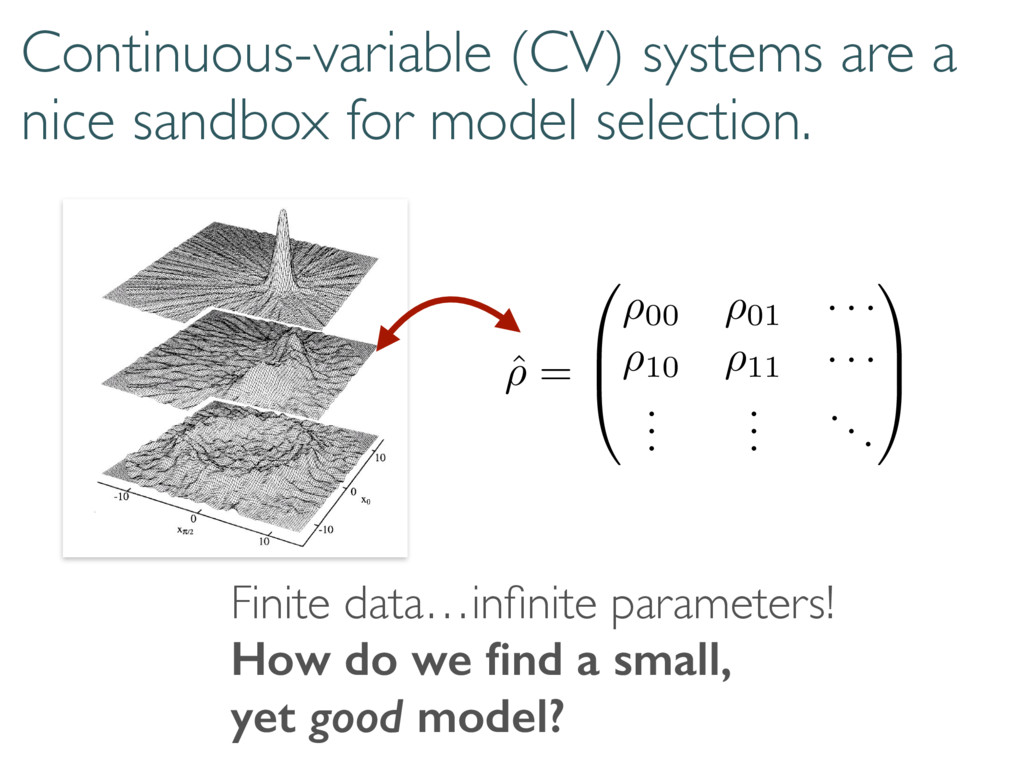
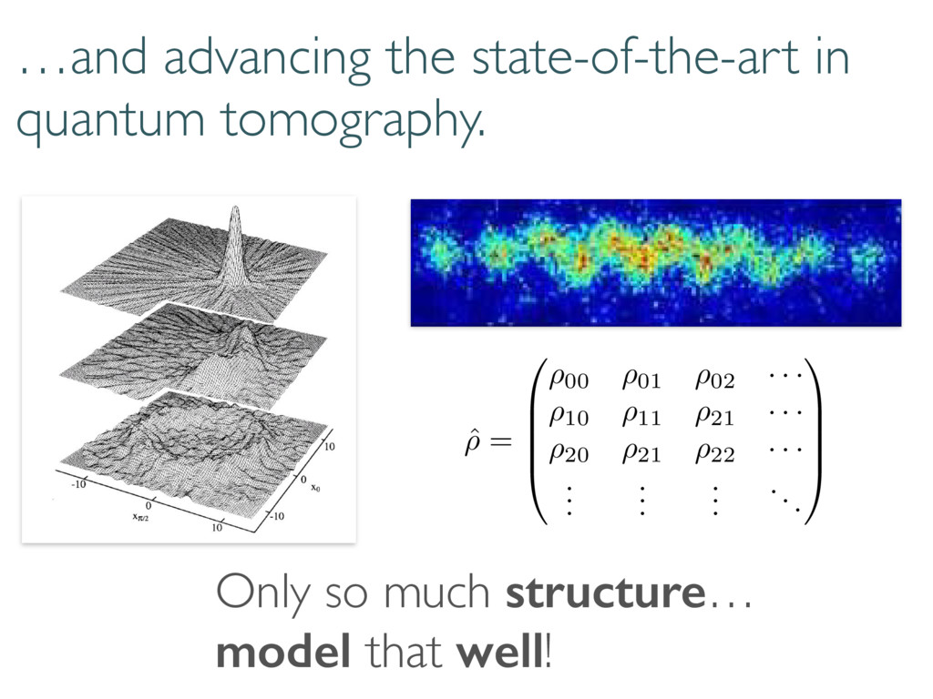
16. ˆ ⇢ = 0 B @ ⇢00 ⇢01 · · · ⇢10 ⇢11 · · · . . . . . . ... 1 C A Continuous-variable (CV) systems are a nice sandbox for model selection. Finite data…infinite parameters! How do we find a small, yet good model?
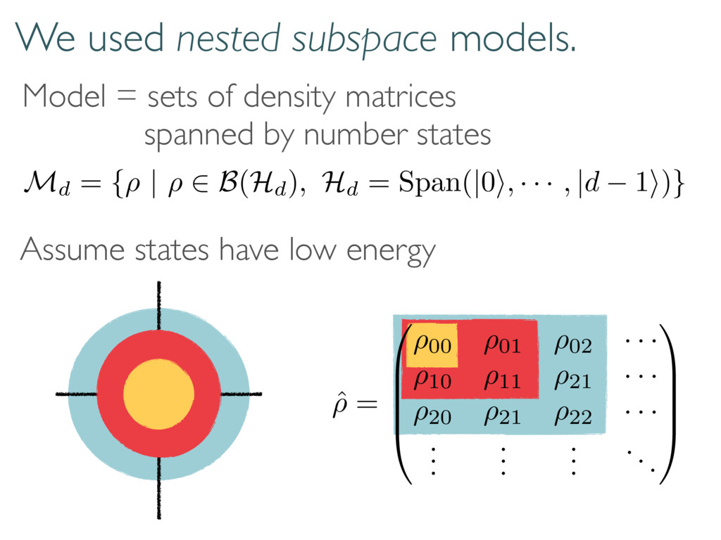
17. We used nested subspace models. ˆ ⇢ = 0 B B B @ ⇢00 ⇢01 ⇢02 · · · ⇢10 ⇢11 ⇢21 · · · ⇢20 ⇢21 ⇢22 · · · . . . . . . . . . ... 1 C C C A Model = sets of density matrices spanned by number states Md = {⇢ | ⇢ 2 B(Hd), Hd = Span(|0i, · · · , |d 1i)} Assume states have low energy
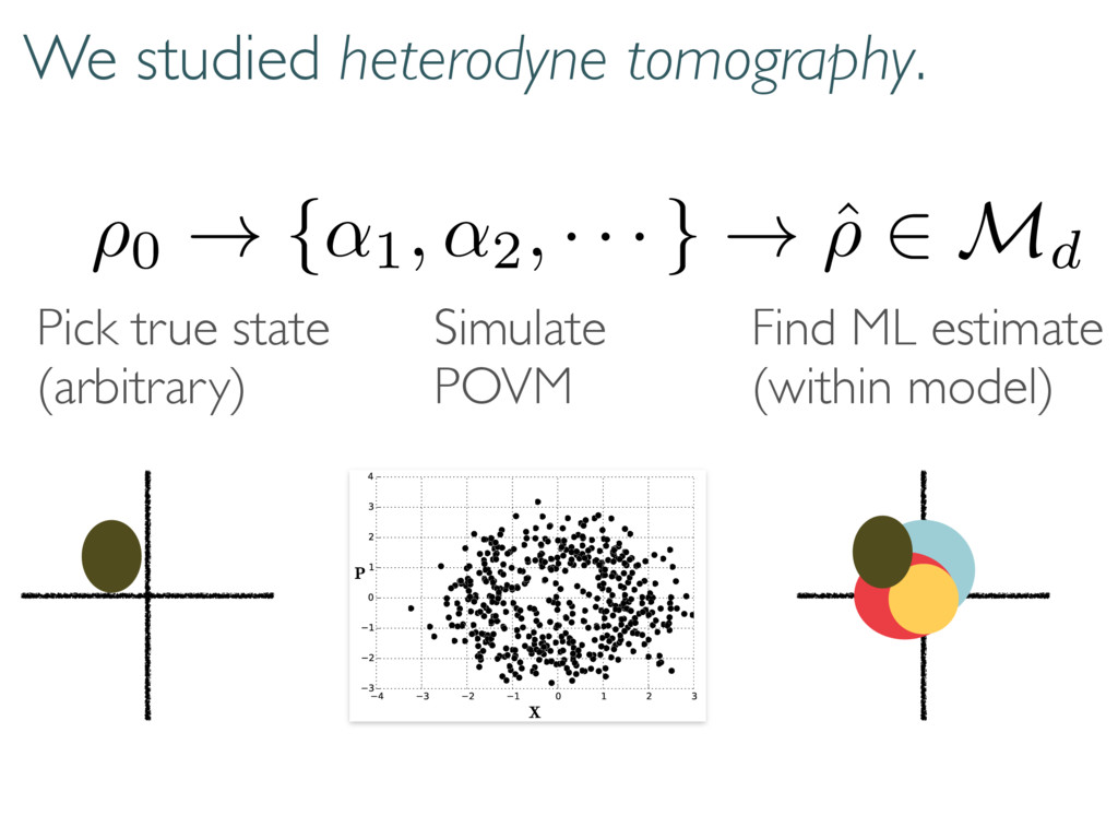
18. We studied heterodyne tomography. ⇢0 ! {↵1, ↵2, · · · } ! ˆ ⇢ 2 Md Pick true state (arbitrary) Simulate POVM Find ML estimate (within model) Doing so in infinite dimensional Hilbert space is harder. From measurements on a continuous variable system, we estimate… 484 Simulated Heterodyne Measurement Outcomes
19. Loglikelihood ratio statistics give us evidence for choosing between models. Compare model to truth with loglikelihood ratios ( ⇢0, Md) = 2 log 0 @ L ( ⇢0) max ⇢2Md L ( ⇢ ) 1 A
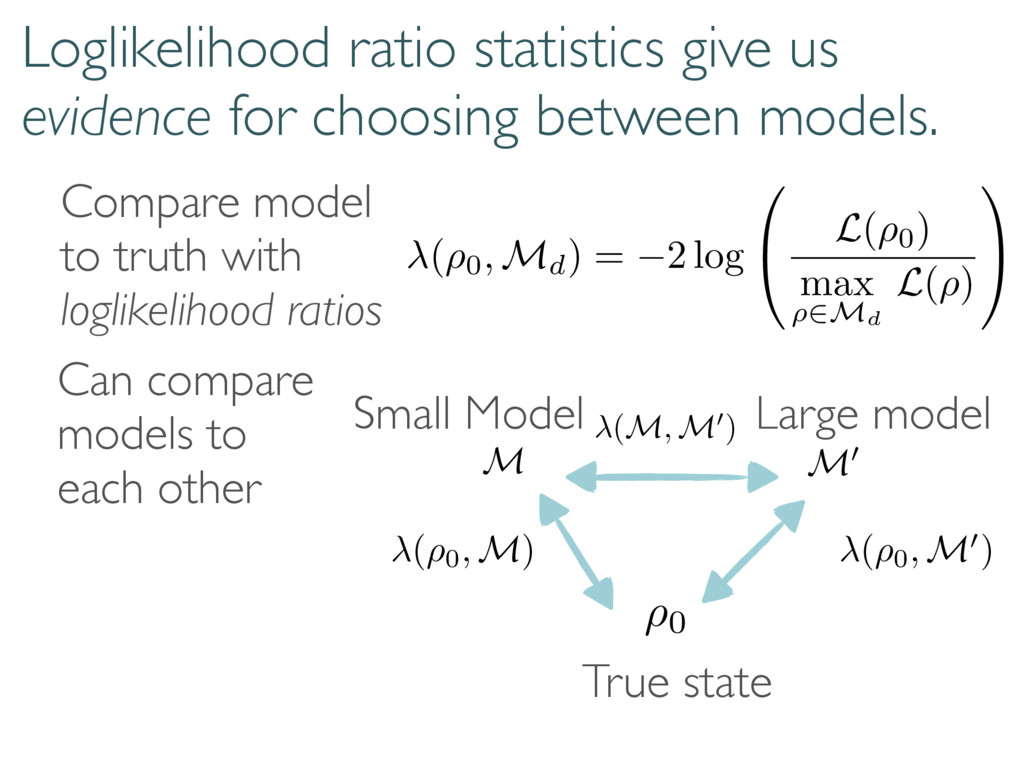
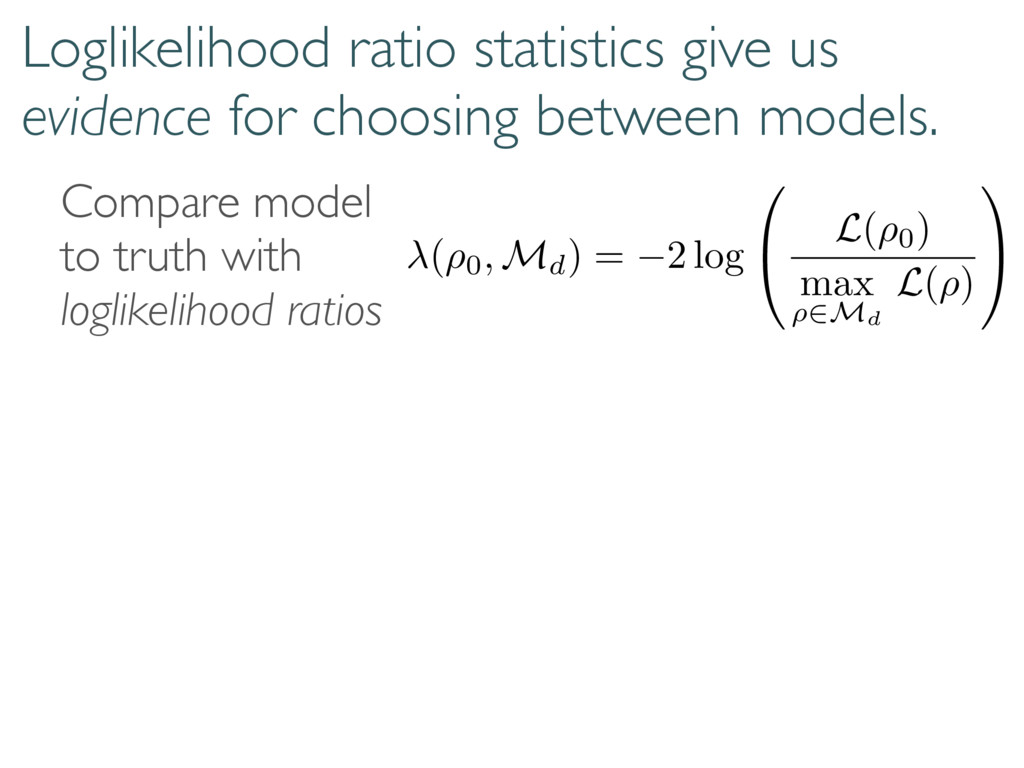
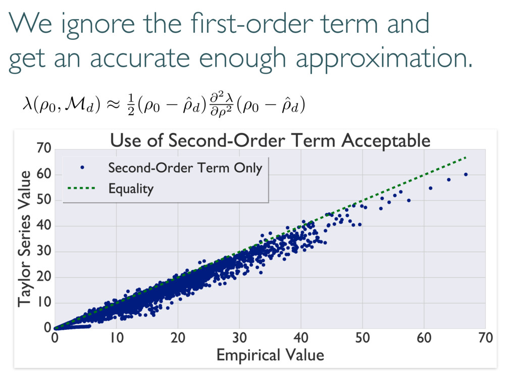
20. Loglikelihood ratio statistics give us evidence for choosing between models. Compare model to truth with loglikelihood ratios ( ⇢0, Md) = 2 log 0 @ L ( ⇢0) max ⇢2Md L ( ⇢ ) 1 A (⇢0, M0) (M, M0) ⇢0 M M0 (⇢0, M) Can compare models to each other True state Small Model Large model
21. Loglikelihood ratio statistics give us evidence for choosing between models. Compare model to truth with loglikelihood ratios ( ⇢0, Md) = 2 log 0 @ L ( ⇢0) max ⇢2Md L ( ⇢ ) 1 A
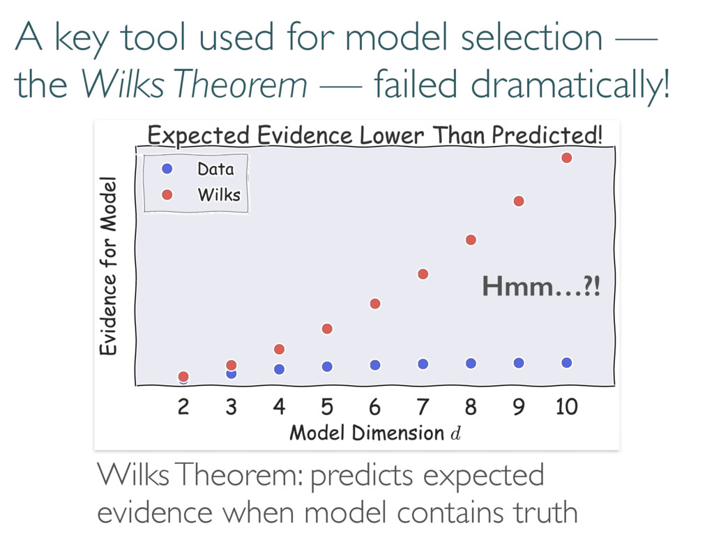
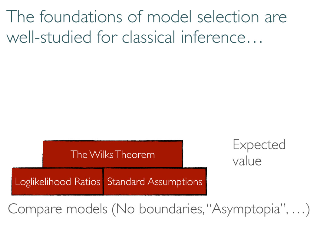
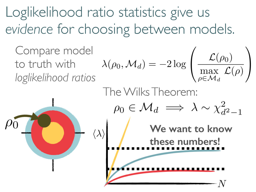
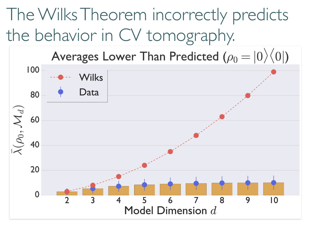
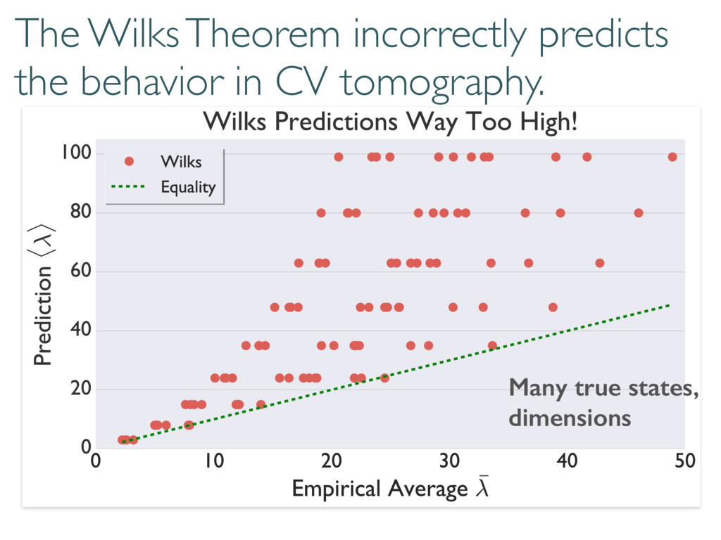
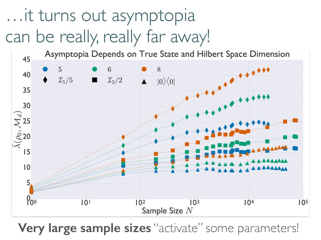
22. Loglikelihood ratio statistics give us evidence for choosing between models. The Wilks Theorem: ⇢0 We want to know these numbers! N h i Compare model to truth with loglikelihood ratios ( ⇢0, Md) = 2 log 0 @ L ( ⇢0) max ⇢2Md L ( ⇢ ) 1 A ⇢0 2 Md =) ⇠ 2 d2 1
23. I thought you said Wilks does not work? Yes. Let’s see the evidence.
24. The Wilks Theorem incorrectly predicts the behavior in CV tomography.
25. The Wilks Theorem incorrectly predicts the behavior in CV tomography. Many true states, dimensions
26. Wilks Theorem gives wrong behavior for the loglikelihood ratio statistic. Wilks Theorem should not be used* for choosing Hilbert space dimension. Let’s fix this. *Nor AIC, etc, because they rely on the Wilks Theorem!
27. Wilks relies on a Taylor series. Let’s start our investigation there. (⇢0, Md) ⇡ r · (⇢0 ˆ ⇢d) + 1 2 (⇢0 ˆ ⇢d) @2 @2⇢ (⇢0 ˆ ⇢d)
28. We ignore the first-order term and get an accurate enough approximation. (⇢0, Md) ⇡ 1 2 (⇢0 ˆ ⇢d)@2 @⇢2 (⇢0 ˆ ⇢d)
29. Let’s cast this equation in a more sensible form. Statistic depends on observed information (H) and fluctuations (F). (⇢0 , Md) ⇡ 1 2 (⇢0 ˆ ⇢d) @2 @⇢2 (⇢0 ˆ ⇢d) ⇡ hh⇢0 ˆ ⇢d |H|⇢0 ˆ ⇢d ii ⇡ Tr(HF) (Superoperators!)
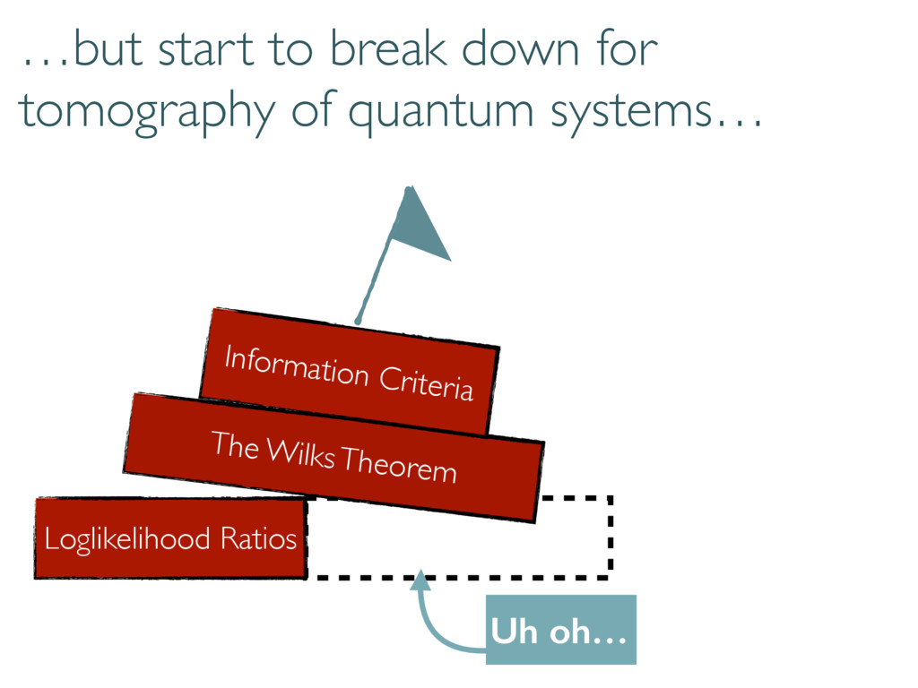
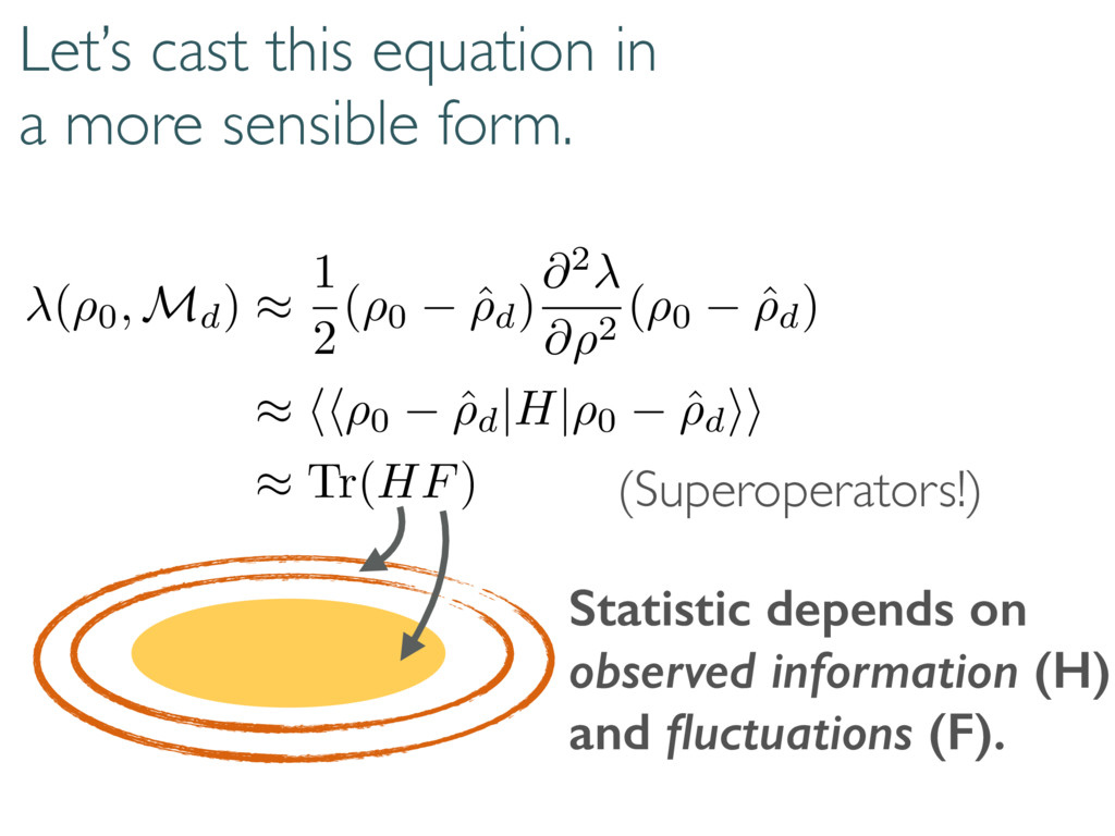
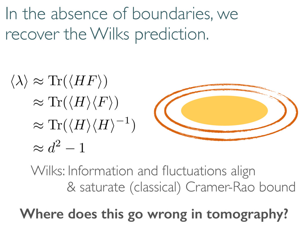
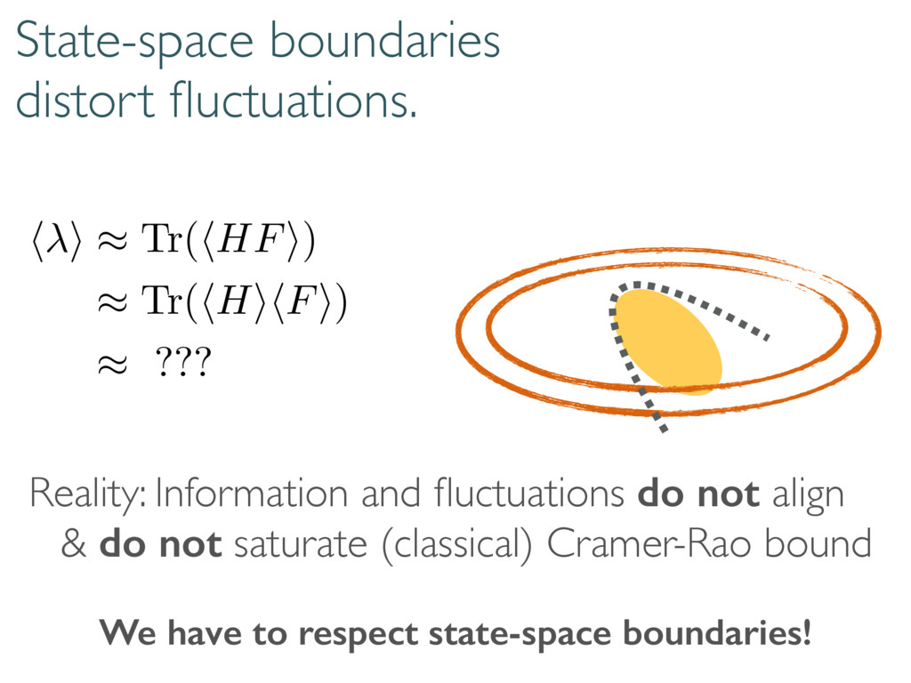
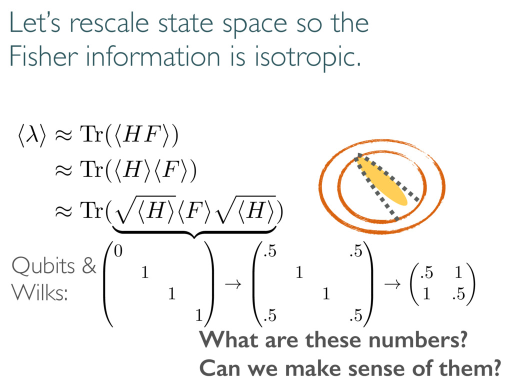
30. In the absence of boundaries, we recover the Wilks prediction. Wilks: Information and fluctuations align & saturate (classical) Cramer-Rao bound Where does this go wrong in tomography? h i ⇡ Tr(hHFi) ⇡ Tr(hHihFi) ⇡ Tr(hHihHi 1) ⇡ d2 1
31. State-space boundaries distort fluctuations. h i ⇡ Tr(hHFi) ⇡ Tr(hHihFi) ⇡ ??? Reality: Information and fluctuations do not align & do not saturate (classical) Cramer-Rao bound We have to respect state-space boundaries!
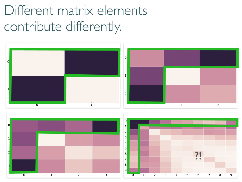
32. Let’s rescale state space so the Fisher information is isotropic. What are these numbers? Can we make sense of them? Qubits & Wilks: h i ⇡ Tr(hHFi) ⇡ Tr(hHihFi) ⇡ Tr( p hHihFi p hHi | {z } ) 0 B B @ 0 1 1 1 1 C C A ! 0 B B @ .5 .5 1 1 .5 .5 1 C C A ! ✓ .5 1 1 .5 ◆
33. Different matrix elements have different contributions. ⇢0 = |0ih0| d = 2 Wilks: One parameter = one unit of expected value!
34. ⇢0 = |0ih0| d = 3 Different matrix elements have different contributions. Wilks: One parameter = one unit of expected value!
35. ⇢0 = |0ih0| d = 4 See a pattern? Different matrix elements have different contributions.
36. Different matrix elements contribute differently. ?!
37. This analysis is borne out in looking at other true states as well. Is there a way to model this behavior?
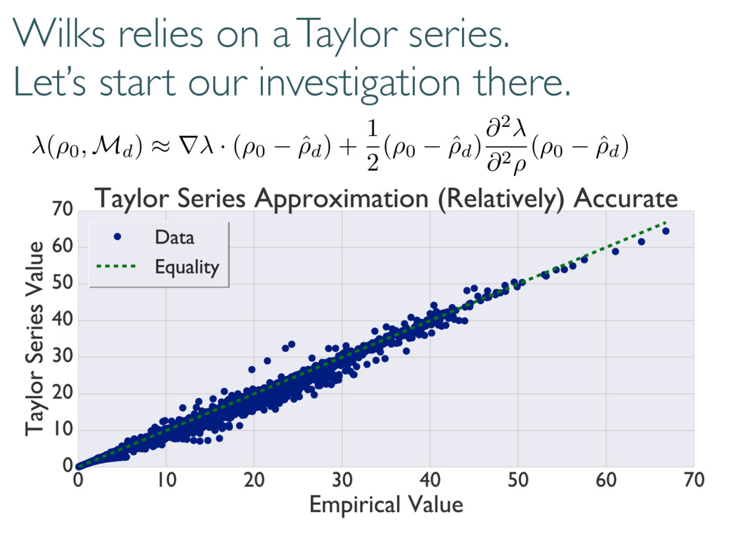
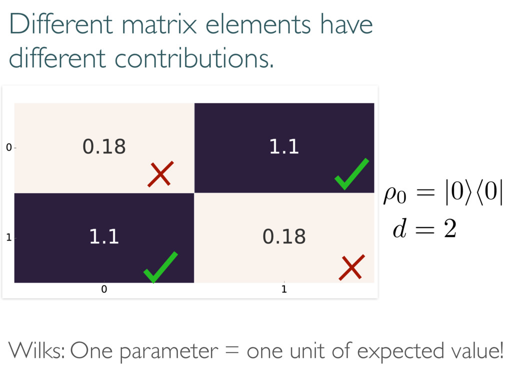
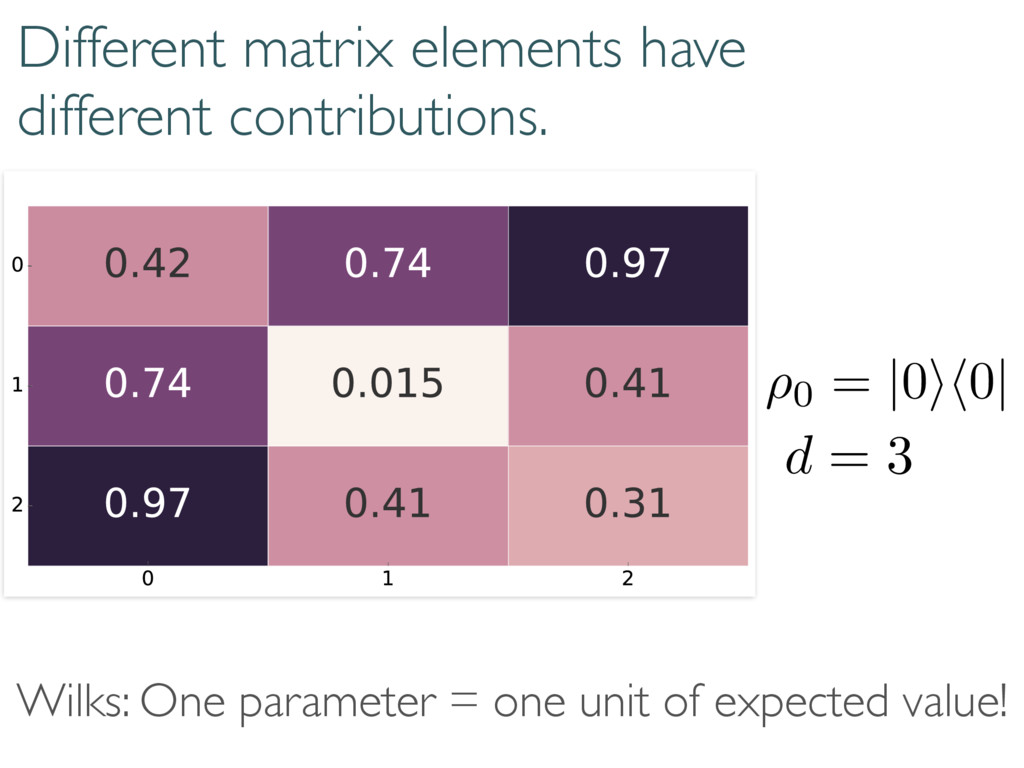
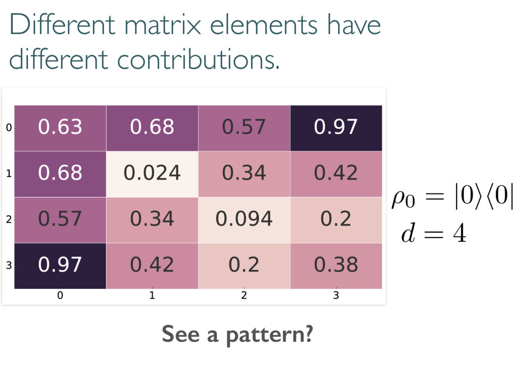
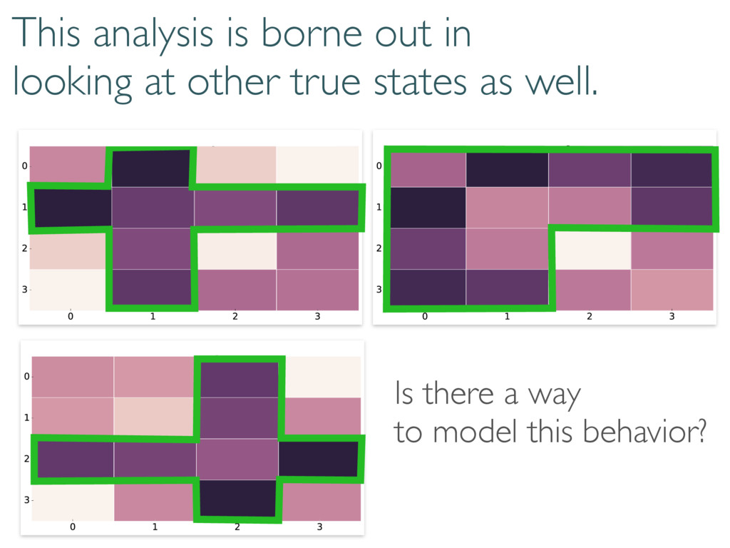
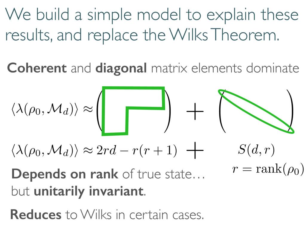
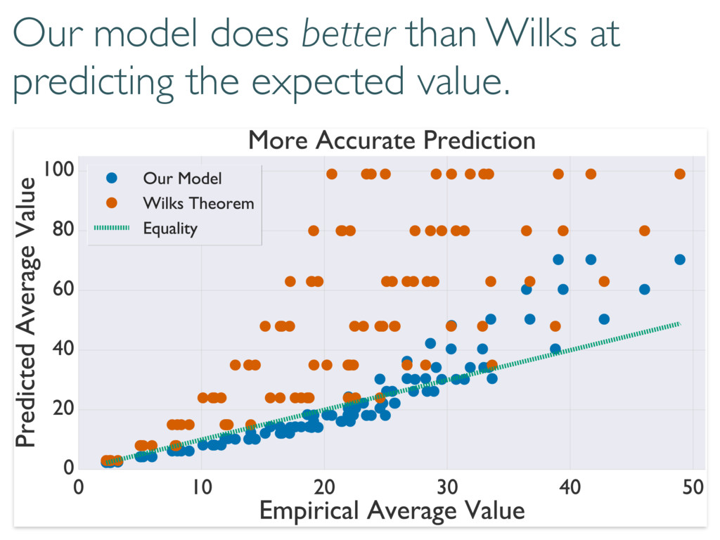
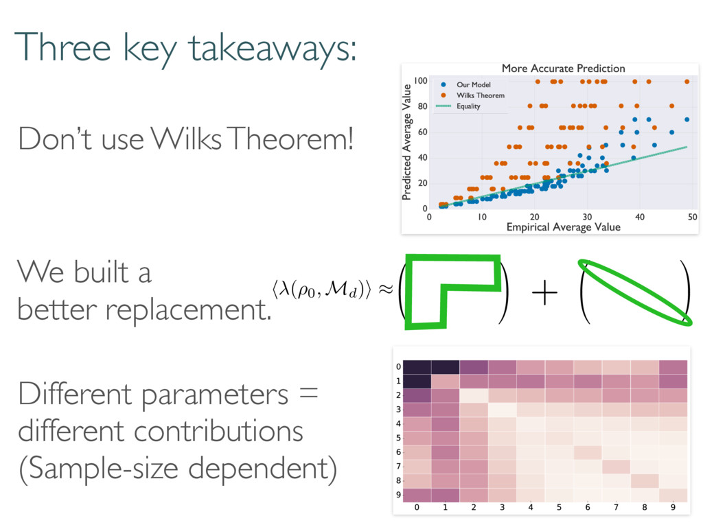
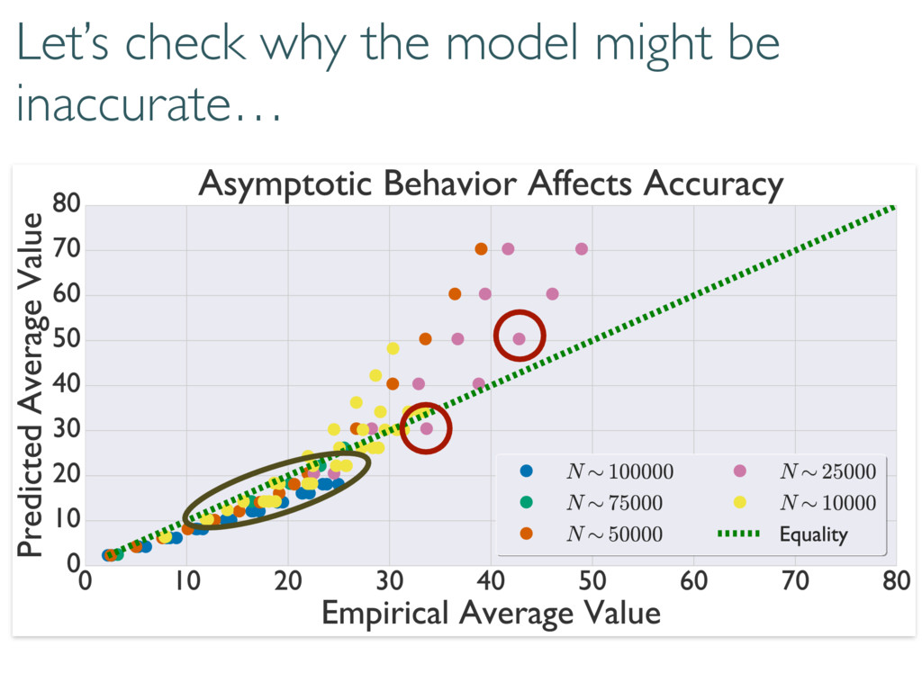
38. We build a simple model to explain these results, and replace the Wilks Theorem. Coherent and diagonal matrix elements dominate 0 @ 1 A 0 @ 1 A + 2rd r(r + 1) S(d, r) Depends on rank of true state… but unitarily invariant. h (⇢0, Md)i ⇡ h (⇢0, Md)i ⇡ + r = rank(⇢0) Reduces to Wilks in certain cases.
39. Our model does better than Wilks at predicting the expected value.
40. Where does this leave us?
41. Three key takeaways: Don’t use Wilks Theorem! We built a better replacement. Different parameters = different contributions (Sample-size dependent) 0 @ 1 A 0 @ 1 A + h (⇢0, Md)i ⇡
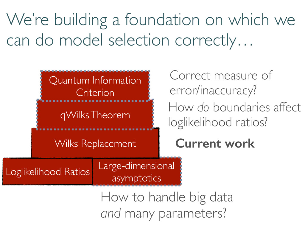
42. We’re building a foundation on which we can do model selection correctly… Large-dimensional asymptotics Wilks Replacement qWilks Theorem Quantum Information Criterion How do boundaries affect loglikelihood ratios? Correct measure of error/inaccuracy? How to handle big data and many parameters? Current work Loglikelihood Ratios
43. …and advancing the state-of-the-art in quantum tomography. Only so much structure… model that well! ˆ ⇢ = 0 B B B @ ⇢00 ⇢01 ⇢02 · · · ⇢10 ⇢11 ⇢21 · · · ⇢20 ⇢21 ⇢22 · · · . . . . . . . . . ... 1 C C C A
44. Thank you! @Travis_Sch
45. Image credits: Wigner function: By Gerd Breitenbach (dissertation) [GFDL (http:// www.gnu.org/copyleft/fdl.html) or CC-BY-SA-3.0 (http:// creativecommons.org/licenses/by-sa/3.0/)], via Wikimedia Commons gmon qubit: By Michael Fang, John Martinis group. http:// web.physics.ucsb.edu/~martinisgroup/photos.shtml NIST Ion Trap: http://phys.org/news/2006-07-ion-large-quantum.html
46. Supplemental Material
47. Let’s check why the model might be inaccurate…
48. …it turns out asymptopia can be really, really far away! Very large sample sizes “activate” some parameters!