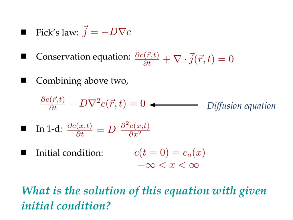
condition: What is the solution of this equation with given initial condition? ~ j = Drc @c(~ r,t) @t + r ·~ j(~ r, t) = 0 @c(~ r,t) @t Dr2c(~ r, t) = 0 @c ( x,t ) @t = D @ 2 c ( x,t ) @x 2 c ( t = 0) = co ( x ) 1 < x < 1 Diffusion equation
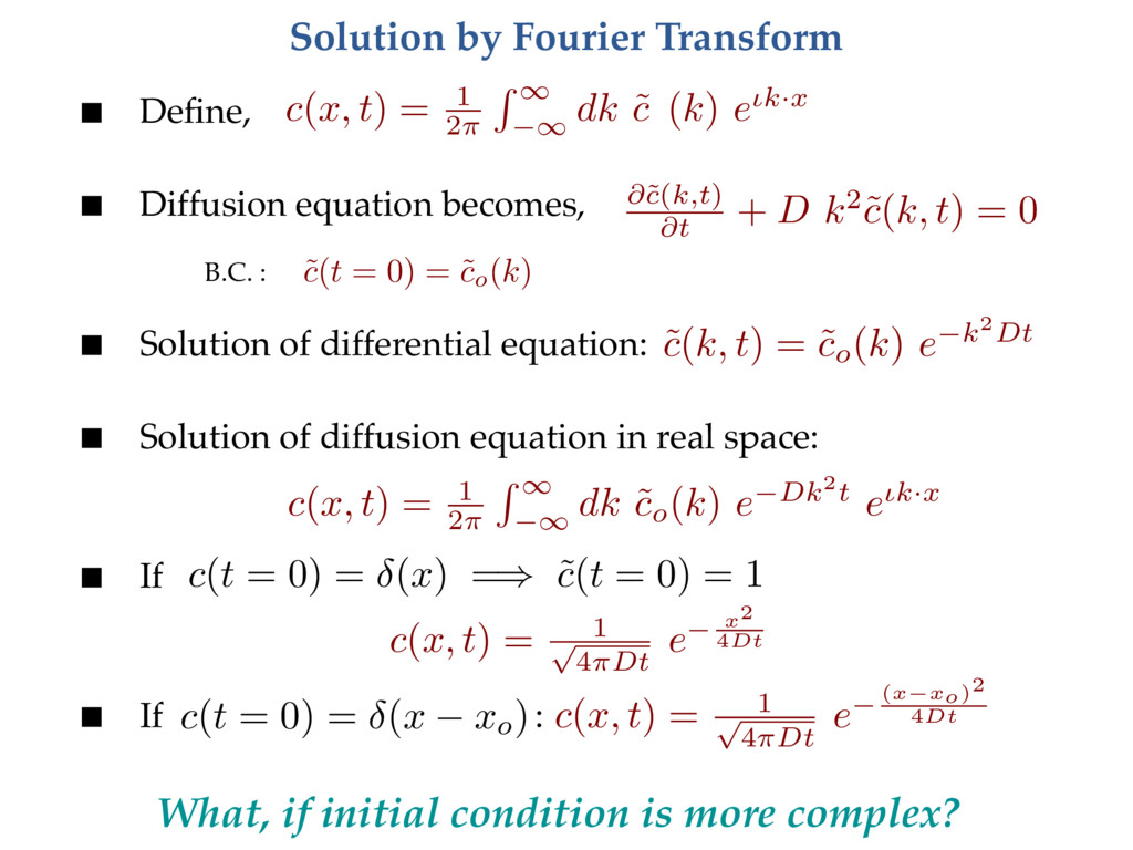
= ˜ c o (k) ˜ c(k, t) = ˜ c o (k) e k 2 Dt c ( x, t ) = 1 p 4⇡Dt e x 2 4 Dt c ( x, t ) = 1 p 4⇡Dt e ( x xo )2 4 Dt c ( x, t ) = 1 2 ⇡ R 1 1 dk ˜ co ( k ) e Dk 2 t e◆k · x c ( x, t ) = 1 2 ⇡ R 1 1 dk ˜ co ( k ) e◆k · x c ( t = 0) = ( x xo ) c ( t = 0) = ( x ) =) ˜ c ( t = 0) = 1 Define, Diffusion equation becomes, Solution of differential equation: Solution of diffusion equation in real space: If If : What, if initial condition is more complex? @˜ c(k,t) @t + D k2˜ c(k, t) = 0
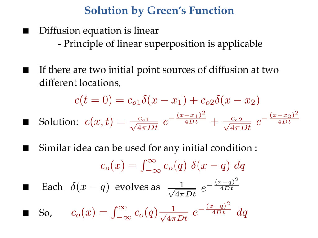
co 1 ( x x1) + co 2 ( x x2) c ( x, t ) = c o 1 p 4⇡Dt e ( x x1)2 4 Dt + c o 2 p 4⇡Dt e ( x x2)2 4 Dt co ( x ) = R 1 1 co ( q ) 1 p 4 ⇡Dt e ( x q )2 4 Dt dq co ( x ) = R 1 1 co ( q ) ( x q ) dq ( x q ) 1 p 4⇡Dt e ( x q )2 4 Dt Diffusion equation is linear - Principle of linear superposition is applicable If there are two initial point sources of diffusion at two different locations, Solution: Similar idea can be used for any initial condition : Each evolves as So,
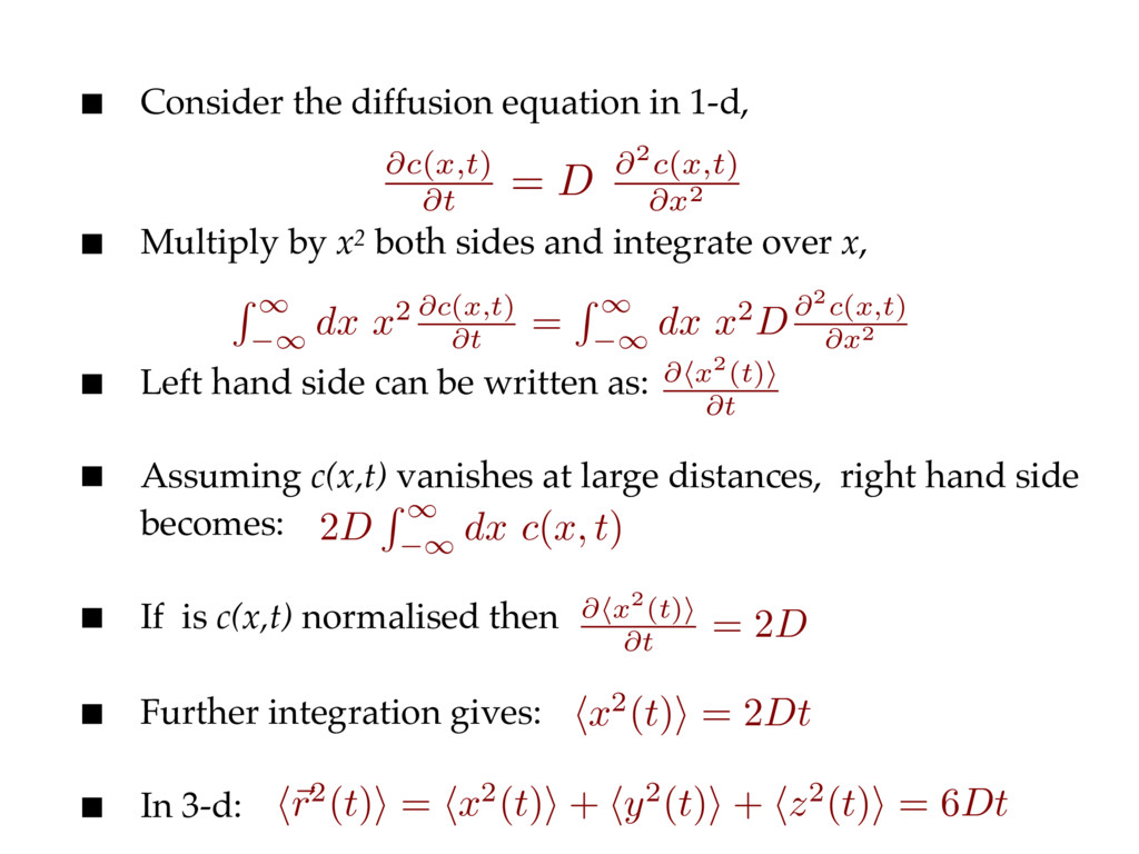
sides and integrate over x, Left hand side can be written as: Assuming c(x,t) vanishes at large distances, right hand side becomes: If is c(x,t) normalised then Further integration gives: In 3-d: @c ( x,t ) @t = D @ 2 c ( x,t ) @x 2 R 1 1 dx x 2 @c ( x,t ) @t = R 1 1 dx x 2 D@ 2 c ( x,t ) @x 2 @ h x 2( t )i @t 2 D R 1 1 dx c ( x, t ) @ h x 2( t )i @t = 2D h x 2( t )i = 2 Dt h ~ r 2( t )i = h x 2( t )i + h y 2( t )i + h z 2( t )i = 6 Dt
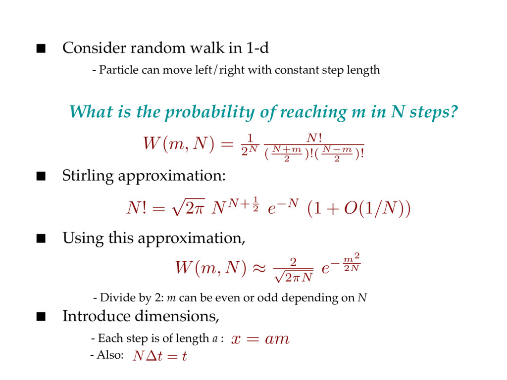
with constant step length What is the probability of reaching m in N steps? Stirling approximation: Using this approximation, - Divide by 2: m can be even or odd depending on N Introduce dimensions, - Each step is of length a : - Also: W(m, N) = 1 2N N! ( N+m 2 )!( N m 2 )! N! = p 2⇡ NN+ 1 2 e N (1 + O(1/N)) W(m, N) ⇡ 2 p 2⇡N e m2 2N x = am N t = t
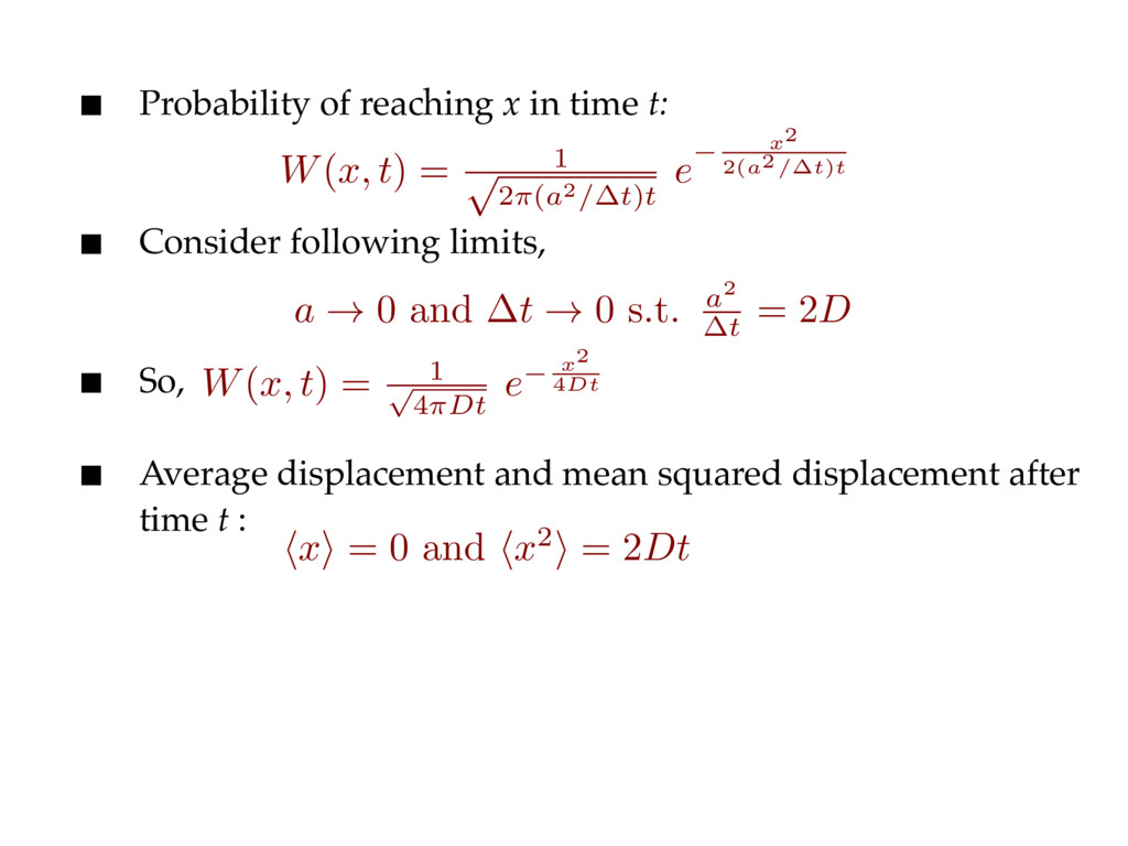
So, Average displacement and mean squared displacement after time t : W ( x, t ) = 1 p 2⇡(a2/ t)t e x 2 2( a 2 / t ) t a ! 0 and t ! 0 s.t. a2 t = 2D W ( x, t ) = 1 p 4⇡Dt e x 2 4 Dt h x i = 0 and h x 2i = 2 Dt
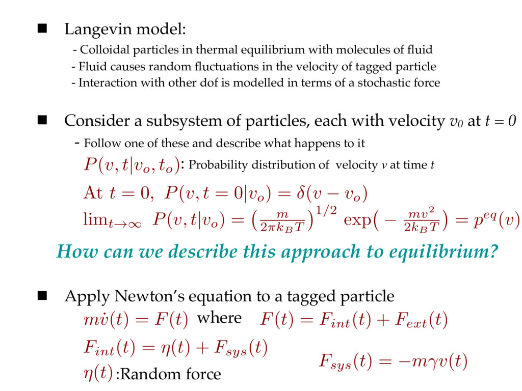
0, P(v, t = 0|v o ) = (v v o ) limt !1 P ( v, t|v o) = m 2 ⇡kBT 1 / 2 exp mv 2 2 kBT = peq ( v ) m˙ v(t) = F(t) F(t) = F int (t) + F ext (t) Fint(t) = ⌘(t) + Fsys(t) Fsys(t) = m v(t) ⌘(t):Random force Langevin model: - Colloidal particles in thermal equilibrium with molecules of fluid - Fluid causes random fluctuations in the velocity of tagged particle - Interaction with other dof is modelled in terms of a stochastic force Consider a subsystem of particles, each with velocity v0 at t = 0 - Follow one of these and describe what happens to it : Probability distribution of velocity v at time t How can we describe this approach to equilibrium? Apply Newton’s equation to a tagged particle where
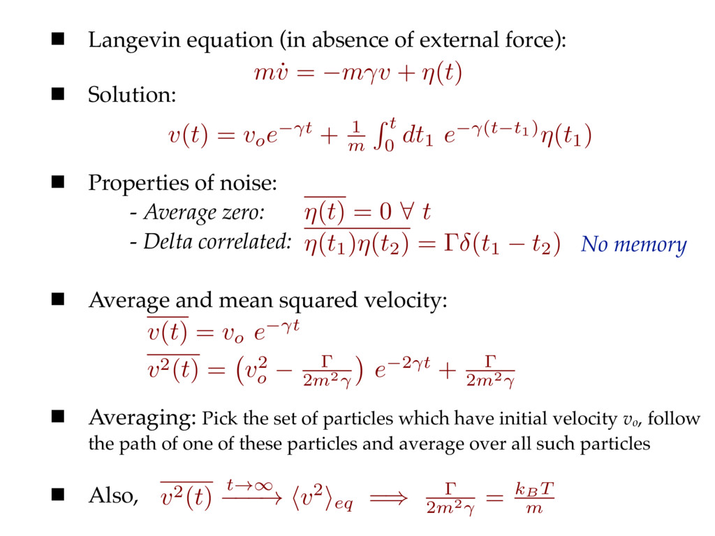
noise: - Average zero: - Delta correlated: Average and mean squared velocity: Averaging: Pick the set of particles which have initial velocity vo, follow the path of one of these particles and average over all such particles Also, m˙ v = m v + ⌘(t) v(t) = v o e t + 1 m R t 0 dt1 e ( t t1)⌘(t1) ⌘(t) = 0 8 t ⌘(t1)⌘(t2) = (t1 t2) v(t) = v o e t v2(t) = v2 o 2 m 2 e 2 t + 2 m 2 v2(t) t!1 ! hv2ieq =) 2m2 = kBT m No memory
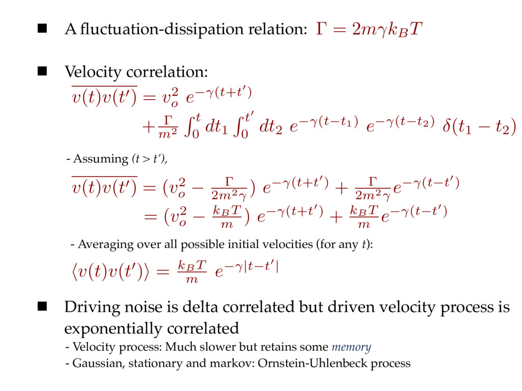
- Averaging over all possible initial velocities (for any t): Driving noise is delta correlated but driven velocity process is exponentially correlated - Velocity process: Much slower but retains some memory - Gaussian, stationary and markov: Ornstein-Uhlenbeck process = 2m kBT v(t)v(t0) = v2 o e ( t + t 0) + m2 R t 0 dt1 R t0 0 dt2 e (t t1) e (t t2) (t1 t2) v(t)v(t0) = (v2 o 2 m 2 ) e ( t + t 0) + 2 m 2 e ( t t 0) = (v2 o kBT m ) e ( t + t 0) + kBT m e ( t t 0) hv(t)v(t0)i = kBT m e |t t0|
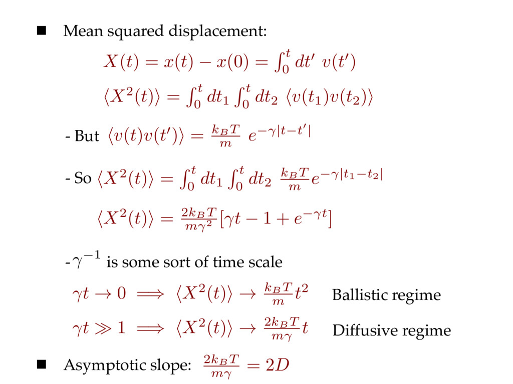
sort of time scale hX2(t)i = R t 0 dt1 R t 0 dt2 hv(t1)v(t2)i X ( t ) = x ( t ) x (0) = R t 0 dt 0 v ( t 0) hv(t)v(t0)i = kBT m e |t t0| hX2(t)i = R t 0 dt1 R t 0 dt2 kBT m e |t1 t2 | hX2(t)i = 2kBT m 2 [ t 1 + e t] 1 t ! 0 =) hX2(t)i ! kBT m t2 t 1 =) hX2(t)i ! 2kBT m t Asymptotic slope: 2kBT m = 2D Ballistic regime Diffusive regime
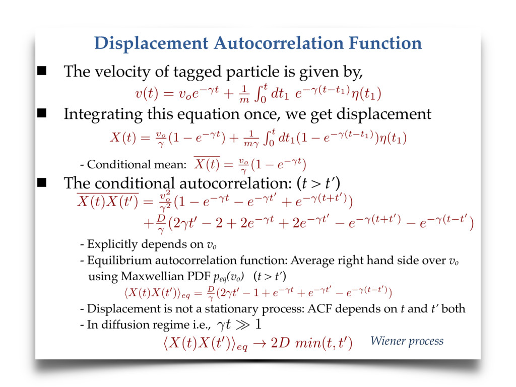
by, Integrating this equation once, we get displacement - Conditional mean: The conditional autocorrelation: (t > t’) - Explicitly depends on vo - Equilibrium autocorrelation function: Average right hand side over vo using Maxwellian PDF peq(vo) (t > t’) - Displacement is not a stationary process: ACF depends on t and t’ both - In diffusion regime i.e., Wiener process X(t) = v o (1 e t) + 1 m R t 0 dt1(1 e (t t1))⌘(t1) X(t) = v o (1 e t) hX(t)X(t0)ieq = D (2 t0 1 + e t + e t0 e (t t0)) t 1 hX(t)X(t0)ieq ! 2D min(t, t0) v(t) = v o e t + 1 m R t 0 dt1 e ( t t1)⌘(t1) +D (2 t0 2 + 2e t + 2e t0 e (t+t0) e (t t0 ) X(t)X(t0) = v2 o 2 (1 e t e t0 + e (t+t0))
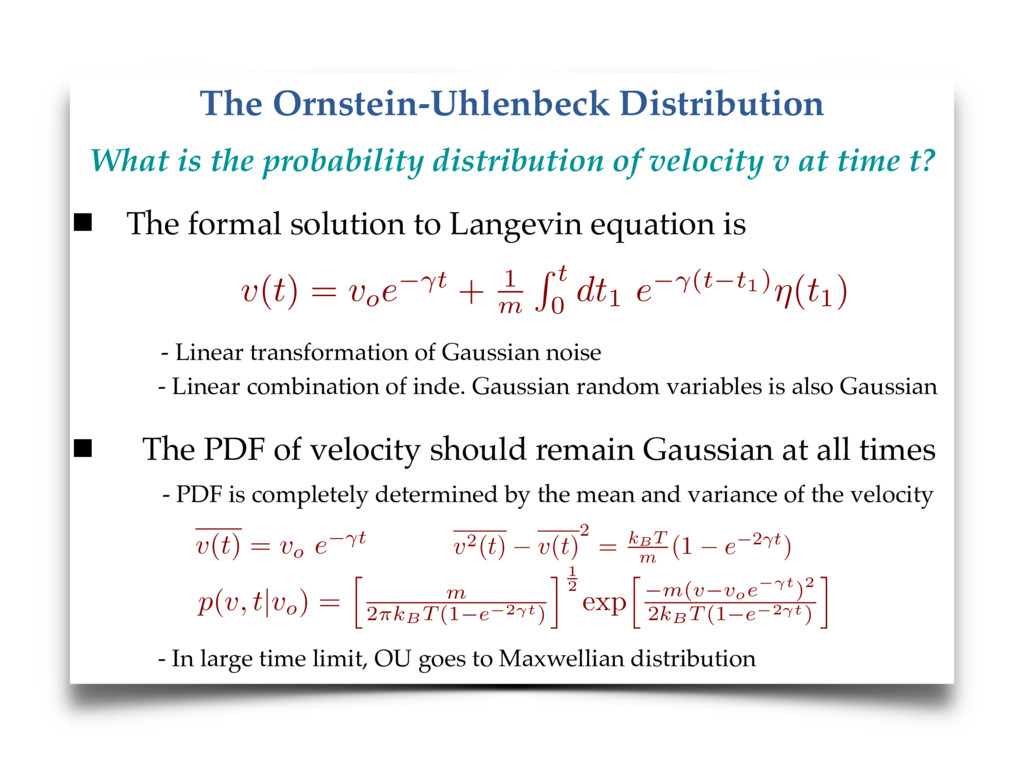
1 m R t 0 dt1 e ( t t1)⌘(t1) The formal solution to Langevin equation is - Linear transformation of Gaussian noise - Linear combination of inde. Gaussian random variables is also Gaussian The PDF of velocity should remain Gaussian at all times - PDF is completely determined by the mean and variance of the velocity - In large time limit, OU goes to Maxwellian distribution v(t) = v o e t v2(t) v(t) 2 = kBT m (1 e 2 t) p ( v, t|v o) = h m 2 ⇡kBT (1 e 2 t ) i1 2 exp h m ( v voe t)2 2 kBT (1 e 2 t ) i What is the probability distribution of velocity v at time t?
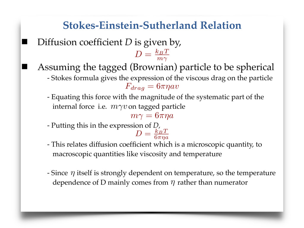
tagged (Brownian) particle to be spherical - Stokes formula gives the expression of the viscous drag on the particle - Equating this force with the magnitude of the systematic part of the internal force i.e. on tagged particle - Putting this in the expression of D, - This relates diffusion coefficient which is a microscopic quantity, to macroscopic quantities like viscosity and temperature - Since itself is strongly dependent on temperature, so the temperature dependence of D mainly comes from rather than numerator D = kBT m Fdrag = 6⇡⌘av m v m = 6⇡⌘a D = kBT 6⇡⌘a ⌘ ⌘
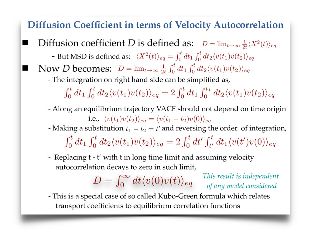
is defined as: - But MSD is defined as: Now D becomes: - The integration on right hand side can be simplified as, - Along an equilibrium trajectory VACF should not depend on time origin i.e., - Making a substitution and reversing the order of integration, - Replacing t - t’ with t in long time limit and assuming velocity autocorrelation decays to zero in such limit, - This is a special case of so called Kubo-Green formula which relates transport coefficients to equilibrium correlation functions D = limt!1 1 2t hX2(t)ieq hX2(t)ieq = R t 0 dt1 R t 0 dt2 hv(t1)v(t2)ieq D = limt!1 1 2t R t 0 dt1 R t 0 dt2 hv(t1)v(t2)ieq R t 0 dt1 R t 0 dt2 hv(t1)v(t2)ieq = 2 R t 0 dt1 R t1 0 dt2 hv(t1)v(t2)ieq hv(t1)v(t2)ieq = hv(t1 t2)v(0)ieq t1 t2 = t0 R t 0 dt1 R t 0 dt2 hv(t1)v(t2)ieq = 2 R t 0 dt0 R t t0 dt1 hv(t0)v(0)ieq This result is independent of any model considered D = R 1 0 dthv(0)v(t)ieq
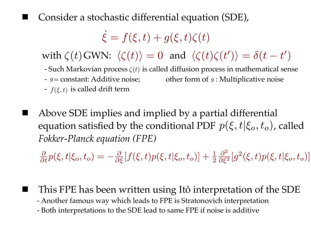
= 0 h⇣(t)⇣(t0)i = (t t0) ⇣(t) g g p(⇠, t|⇠ o , t o ) @ @t p(⇠, t|⇠ o , t o ) = @ @⇠ [f(⇠, t)p(⇠, t|⇠ o , t o )] + 1 2 @ 2 @⇠ 2 [g2(⇠, t)p(⇠, t|⇠ o , t o )] f(⇠, t) Consider a stochastic differential equation (SDE), with GWN: and - Such Markovian process is called diffusion process in mathematical sense - = constant: Additive noise; other form of : Multiplicative noise - is called drift term Above SDE implies and implied by a partial differential equation satisfied by the conditional PDF , called Fokker-Planck equation (FPE) This FPE has been written using Ito interpretation of the SDE - Another famous way which leads to FPE is Stratonovich interpretation - Both interpretations to the SDE lead to same FPE if noise is additive ^
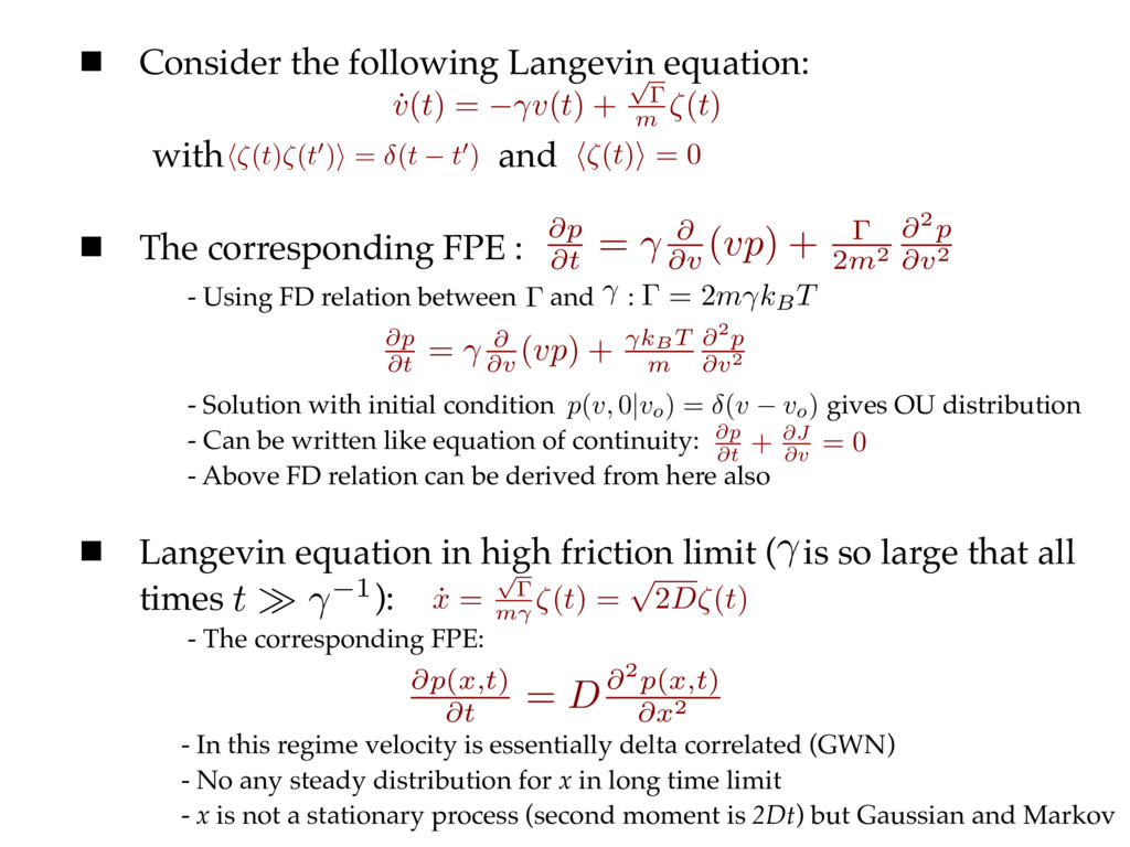
(t t0) h⇣(t)i = 0 @p @t = @ @v (vp) + 2m2 @2p @v2 Consider the following Langevin equation: with and The corresponding FPE : - Using FD relation between and : - Solution with initial condition gives OU distribution - Can be written like equation of continuity: - Above FD relation can be derived from here also Langevin equation in high friction limit ( is so large that all times ): - The corresponding FPE: - In this regime velocity is essentially delta correlated (GWN) - No any steady distribution for x in long time limit - x is not a stationary process (second moment is 2Dt) but Gaussian and Markov @p @t = @ @v (vp) + kBT m @2p @v2 = 2m kBT p(v, 0|v o ) = (v v o ) @p @t + @J @v = 0 t 1 ˙ x = p m ⇣ ( t ) = p 2 D⇣ ( t ) @p ( x,t ) @t = D@ 2 p ( x,t ) @x 2
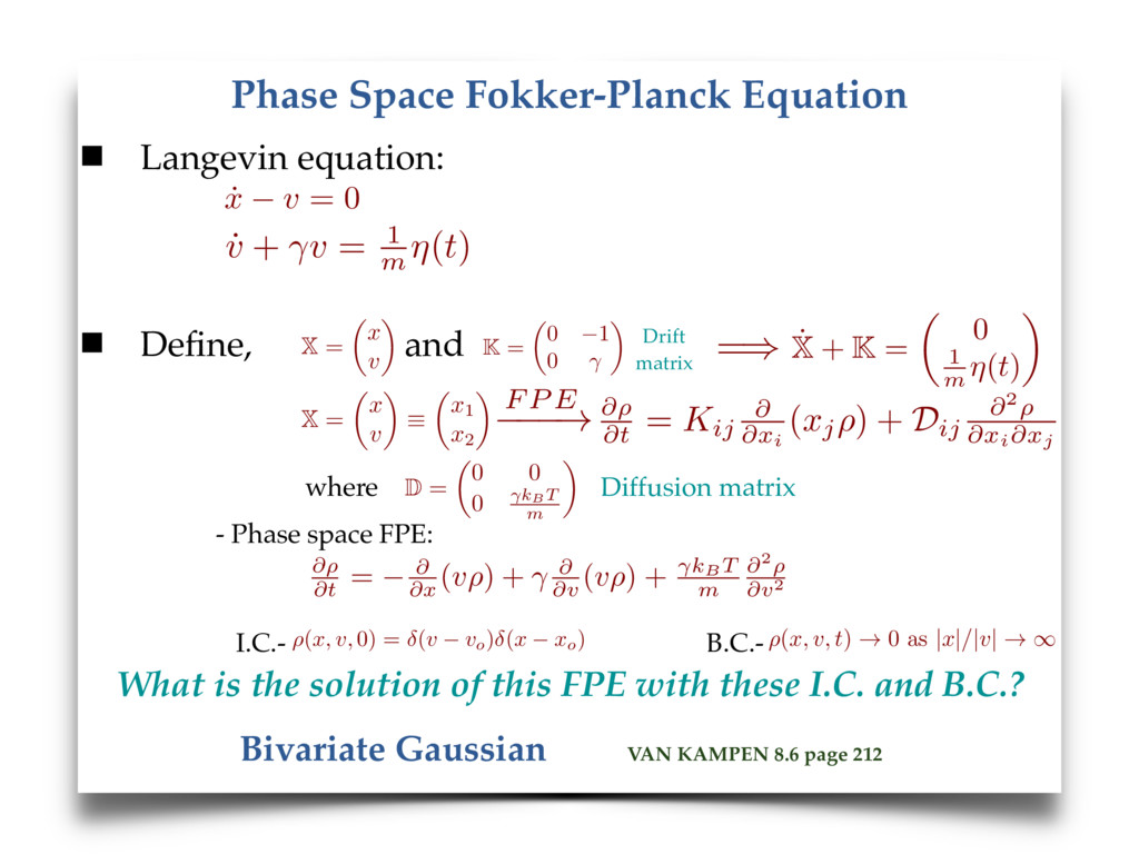
matrix - Phase space FPE: I.C.- B.C.- What is the solution of this FPE with these I.C. and B.C.? ˙ x v = 0 @⇢ @t = Kij @ @xi ( xj⇢ ) + D ij @ 2 ⇢ @xi@xj @⇢ @t = @ @x (v⇢) + @ @v (v⇢) + kBT m @ 2 ⇢ @v 2 X = ✓ x v ◆ K = ✓ 0 1 0 ◆ X = ✓ x v ◆ ⌘ ✓ x1 x2 ◆ F P E ! =) D = ✓ 0 0 0 kBT m ◆ Drift matrix ⇢ ( x, v, 0) = ( v vo ) ( x xo ) ⇢ ( x, v, t ) ! 0 as | x | / | v | ! 1 Bivariate Gaussian VAN KAMPEN 8.6 page 212 ˙ v + v = 1 m ⌘(t) ˙ X + K = ✓ 0 1 m ⌘(t) ◆
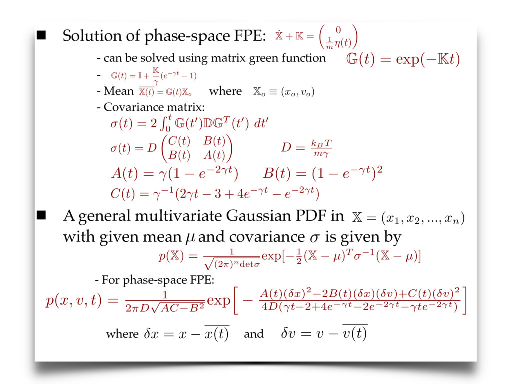
green function - - Mean where - Covariance matrix: A general multivariate Gaussian PDF in with given mean and covariance is given by - For phase-space FPE: where and ˙ X + K = ✓ 0 1 m ⌘(t) ◆ G ( t ) = exp( Kt ) G(t) = I + K (e t 1) X(t) = G(t)X o (t) = 2 R t 0 G(t0)DGT (t0) dt0 X o ⌘ ( xo, vo ) (t) = D ✓ C(t) B(t) B(t) A(t) ◆ D = kBT m A(t) = (1 e 2 t) C(t) = 1(2 t 3 + 4e t e 2 t) B(t) = (1 e t)2 µ X = ( x1, x2, ..., xn) p ( X ) = 1 p (2⇡)ndet exp[ 1 2 ( X µ ) T 1 ( X µ )] x = x x ( t ) v = v v(t) p(x, v, t) = 1 2 ⇡D p AC B 2 exp h A ( t )( x )2 2 B ( t )( x )( v )+ C ( t )( v )2 4 D ( t 2+4 e t 2 e 2 t te 2 t) i
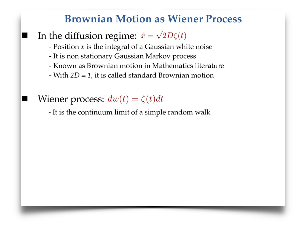
Position x is the integral of a Gaussian white noise - It is non stationary Gaussian Markov process - Known as Brownian motion in Mathematics literature - With 2D = 1, it is called standard Brownian motion Wiener process: - It is the continuum limit of a simple random walk ˙ x = p 2 D⇣ ( t ) dw(t) = ⇣(t)dt
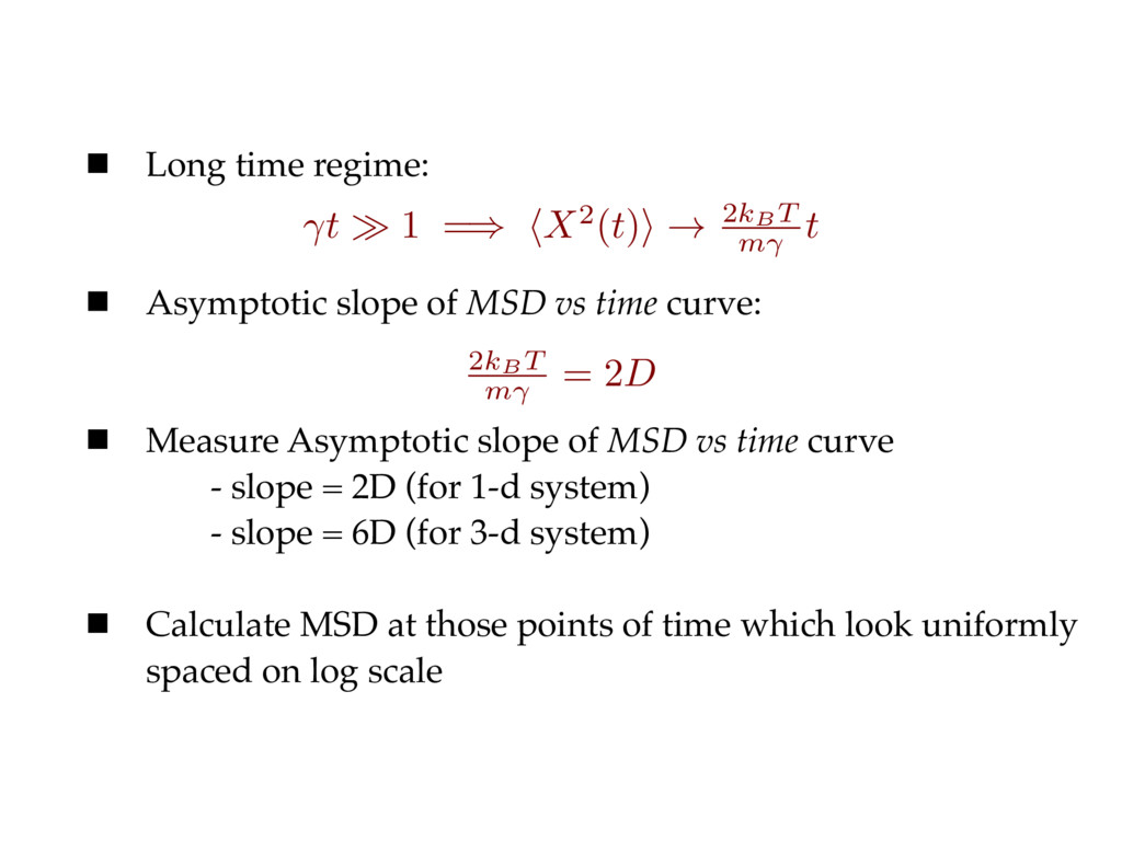
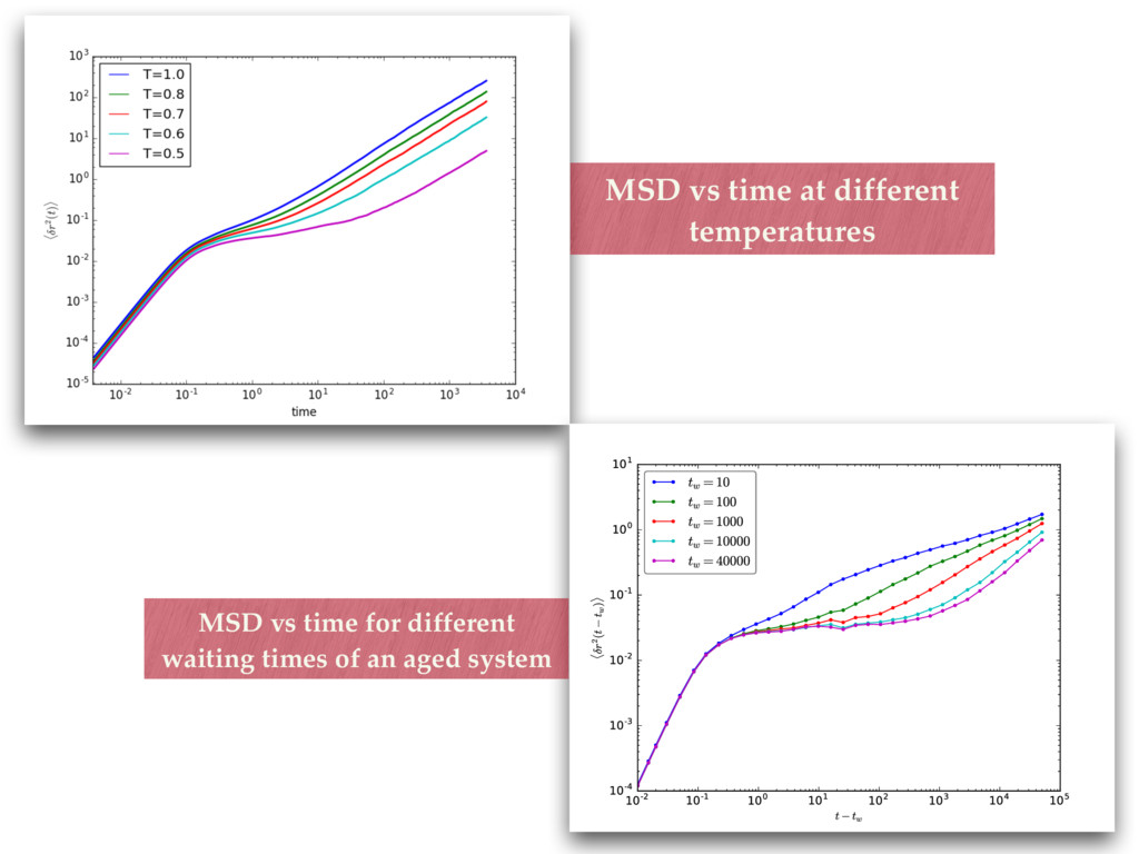
Measure Asymptotic slope of MSD vs time curve - slope = 2D (for 1-d system) - slope = 6D (for 3-d system) Calculate MSD at those points of time which look uniformly spaced on log scale t 1 =) hX2(t)i ! 2kBT m t 2kBT m = 2D