Intro to Reinforcement Learning

Transcript

1. Intro to Reinforcement Learning Yuchu Luo Thursday, 23 August 2017 Computer Animation and Multimedia Analysis LAB Summer Machine Learning Class
2. Supervised Learning: Unsupervised Learning: Reinforcement Learning: y = f (x) Find f (function approximation) f (x) Find f (clusters description) y = f (x),z Find f (that generate y)
3. Example: The Grid World Noisy movement: actions do not always go as planned ✤ 80% of the time, the action North takes the agent North 
 (if there is no wall there) ✤ 10% of the time, North takes the agent West, 10% East ✤ If there is a wall in the direction the agent would have been taken, the agent stays put The agent receives rewards each time step ✤ Small “living” reward each step (can be negative) ✤ Big rewards come at the end (good or bad) Goal: maximize sum of rewards
4. Markov Decision Processes States: Model: Actions: Reward: Policy: T(s,a,s') ~ Pr(s' | s,a) s ∈S a ∈A R(s,a) = E[R t+1 | s,a] π(s)→ a, !* < S,A,R,P >
5. Markov Decision Processes “Markov” means Only Present Matter and Stationary Distribution P(S t+1 = s' | S t = s t ,A t = a t ,S t−1 = s t−1 ,A t−1 ,S 0 = s 0 ) P(S t+1 = s' | S t = s t ,A t = a t ) =
6. Markov Reward Processes +6 -6 t=0 t=1 t=2 t=3 ✤ delay reward ✤ minor changes matter +1 +1 How to find the optimal plan (policy π*)?
7. How to calculate the lone-term total reward? Sequences of Rewards ✤ Infinite Horizons ✤ Utility of Sequences R(s) = -0.3 How to find the optimal plan (policy π*)? π(s)→ a U(s 0 s 1 s 2 ...) = R(s t ) t=0 ∞ ∑
8. +1 +1 +1 +1 +1 … +1 +1 +2 +1 +2 … U(s 0 s 1 s 2 ...) = R(s t ) t=0 ∞ ∑ Non-stationarity X U(s 0 s 1 s 2 ...) = γ t R(s t ) t=0 ∞ ∑ ≤ γ t R max t=0 ∞ ∑ = R max 1−γ Discount 0 ≤ γ <1
9. Recap: Defining MDPs States: Model: Actions: Reward: Policy: Utility: T(s,a,s') ~ Pr(s' | s,a) s ∈S a ∈A R(s,a) = E[R t+1 | s,a] π(s)→ a, !* U(s 0 s 1 s 2 ...) = γ t R(s t ) t=0 ∞ ∑ ≤ γ t R max t=0 ∞ ∑ = R max 1−γ a s s, a s,a,s’ s’
10. Solving MDPs a s s’ s, a (s,a,s’) is a 
 transition s,a,s’ s is a state (s, a) is a q-state ✤ The value (utility) of a state s: V*(s) = expected utility starting in s and acting optimally ✤ The value (utility) of a q-state (s,a): Q*(s,a) = expected utility starting out having taken action a from state s and (thereafter) acting optimally ✤ The optimal policy: !*(s) = optimal action from state s V(s) = E[U t | S t = s] Q(s,a) = E[U t | S t = s,A t = a]
11. State-Value Function Q-Value Function
12. The Bellman Equations V*(s) = max a Q*(s,a) Q*(s,a) = E[U t | S t = s,A t = a] = R s a +γ P ss' a s'∈S ∑ max a' Q*(s',a') Value Iteration V k+1 (s) ← T(s,a,s')[R(s,a,s')+γV k (s')] s' ∑ (Convergent) Q k+1 (s,a) ← T(s,a,s') s' ∑ [R(s,a,s')+γ max a' Q k (s',a')]
13. Finding Policies (via Value Iteration) π *(s) = argmax a Q*(s,a) ✤ Slow ✤ The “max” at each state rarely changes ✤ The policy often converges long before the values
15. 0.72 = 0.8*0.9*1.00 + 0.2*0.9*0.00 0.8, 0.2 from T(s,a,s’), 0.9 is discount V k+1 (s) ← T(s,a,s')[R(s,a,s')+γV k (s')] s' ∑
16. 0.52=0.8*0.9*0.72 + 0.2*0.9*0.00 V k+1 (s) ← T(s,a,s')[R(s,a,s')+γV k (s')] s' ∑
26. Policy Iteration Evaluation Improvement Step 1 Step 2 Calculate utilities for fixed policy Select action when Q-Value > State-Value
27. Agent Environment Actions: a Reward: r State: s Reinforcement Learning
28. Example: Learning to Walk Initial [Kohl and Stone, ICRA 2004]
29. Example: Learning to Walk Training [Kohl and Stone, ICRA 2004]
30. Example: Learning to Walk Finished [Kohl and Stone, ICRA 2004]
31. MDPs and RL ✤ Common ideas: ✤ A set of states s ∈ S ✤ A set of actions (per state) A ✤ A model T(s,a,s’) ✤ A reward function R(s,a,s’) ✤ Still looking for a policy !(s) ✤ New twist: don’t know T or R ✤ I.e. we don’t know which states are good or what the actions do ✤ Must actually try actions and states out to learn
32. MDPs and RL MDPs (Offline) RL (Online)
33. Model-Based Learning Step 1: learn a model of how the environment works from its observations Step 2: plan a solution using that model ˆ T(s,a,s') ˆ R(s,a,s') Learn and through (s, a, s’) pairs. For example, use value iteration solve the learned MDP as before.
34. Example: Expected Age Known P(A) E[A] = P(a)⋅a a ∑ = 0.3×18 +... Unknown P(A): “Model Based” ˆ P(a) = num(a) N E[A] ≈ ˆ P(a)⋅a a ∑ Unknown P(A): “Model Free” E[A] ≈ 1 N a i i ∑ Without P(A), instead collect samples [a1, a2, … aN]
35. Model-Free Learning
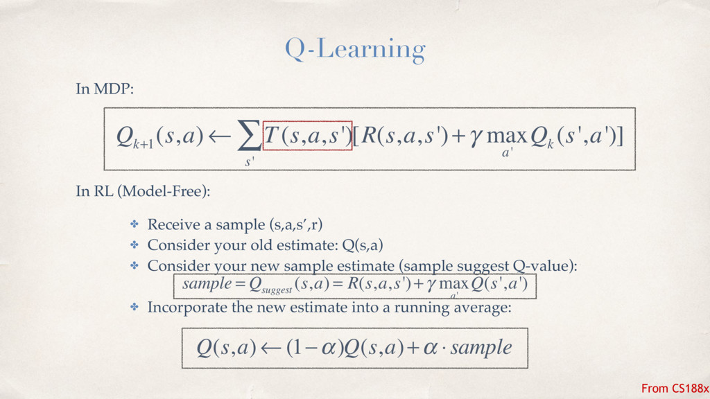
36. Q k+1 (s,a) ← T(s,a,s') s' ∑ [R(s,a,s')+γ max a' Q k (s',a')] Q-Learning In MDP: In RL (Model-Free): ✤ Receive a sample (s,a,s’,r) ✤ Consider your old estimate: Q(s,a) ✤ Consider your new sample estimate (sample suggest Q-value): ✤ Incorporate the new estimate into a running average: Q(s,a) ← (1−α)Q(s,a)+α ⋅sample sample = Q suggest (s,a) = R(s,a,s')+γ max a' Q(s',a') From CS188x
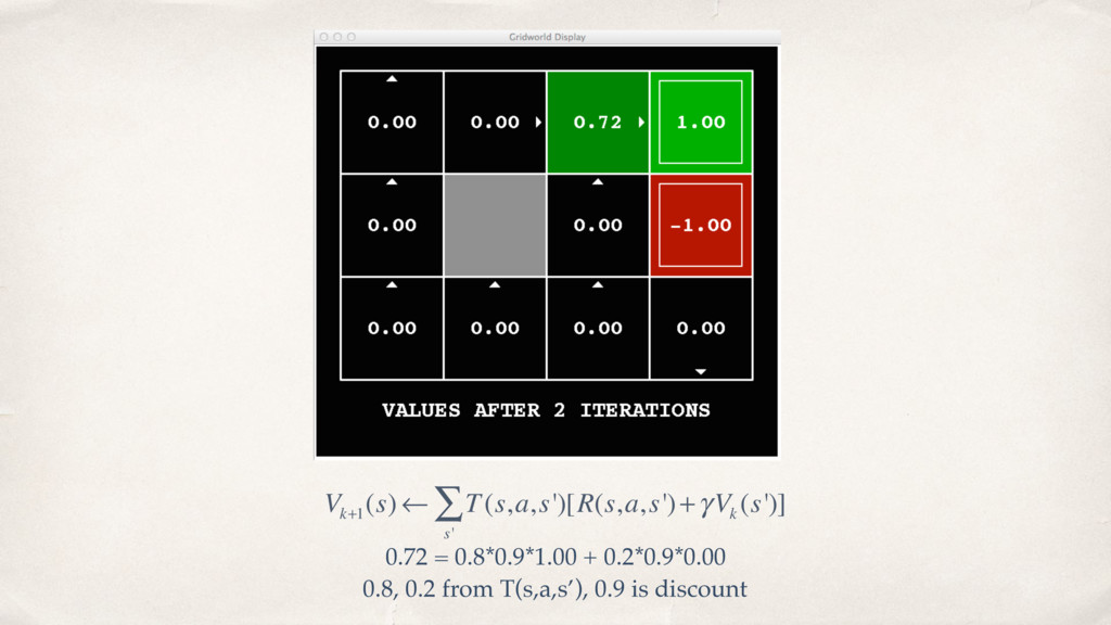
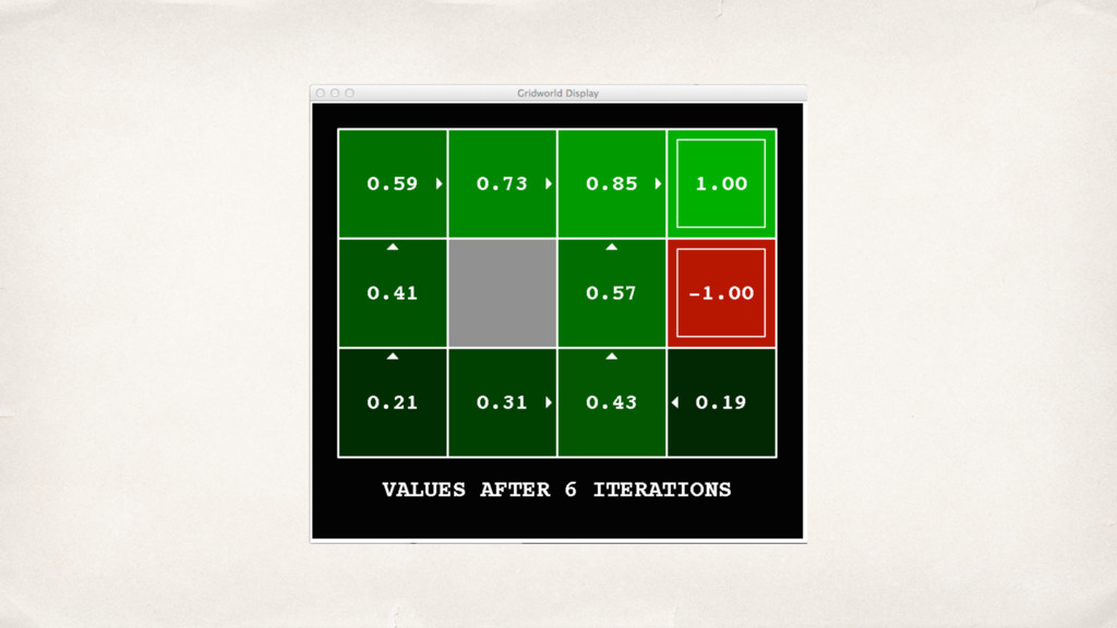
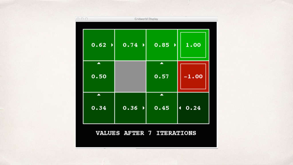
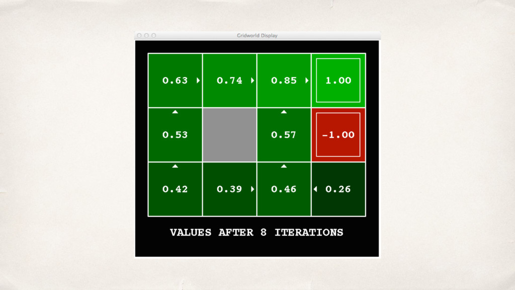
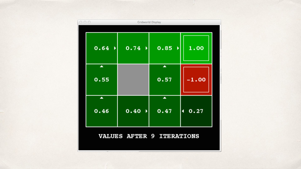
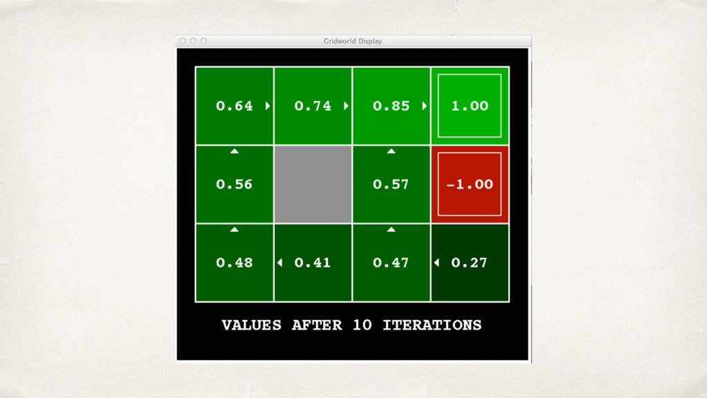
38. Exploration and Exploitation python gridworld.py -m -v -g BridgeGrid -p -a q -k 100 -n 0 How to Explore? Random Actions (ε-greedy) ✤ Every time step, flip a coin ✤ With (small) probability ε, act randomly ✤ With (large) probability 1-ε, act on current policy ✤ Lower ε over time
39. Approximate Q-Learning The Problem: ✤ Too many states to visit ✤ Too many states to hold the q-tables in memory
40. Feature-Based Representations ✤ Solution: describe a state using a vector of features (properties) ✤ Features are functions from states to real numbers (often 0/1) that capture important properties of the state ✤ Example features: ✤ Distance to closest ghost ✤ Distance to closest dot ✤ Number of ghosts ✤ 1 / (dist to dot)2 ✤ Is Pacman in a tunnel? (0/1) ✤ …… etc. ✤ Is it the exact state on this slide? ✤ Can also describe a q-state (s, a) with features (e.g. action moves closer to food)
41. Linear Value Functions Approximate Q-Learning difference = [r +γ max a' Q(s',a')]−Q(s,a) Update Q(s,a) ← Q(s,a)+α ⋅difference w i ← w i +α ⋅difference⋅ f i (s,a)
42. Example: Q-Pacman
44. Next time: Deep Reinforcement Learning