ABC using Linear Discriminant Analysis

slides of a talk given by Jean-Michel Marin at ISBA 2012, in Kyoto

Transcript

1. Estimation of demo-genetic model probabilities with Approximate Bayesian Computation using linear discriminant analysis on summary statistics Jean-Michel Marin Institut de Math´ ematiques et Mod´ elisation Universit´ e Montpellier 2 Joint work with Arnaud Estoup, ´ Eric Lombaert, Thomas Guillemaud, Pierre Pudlo, Christian P. Robert, Jean-Marie Cornuet ISBA 2012, Kyoto, June 28, 2012 Page 1
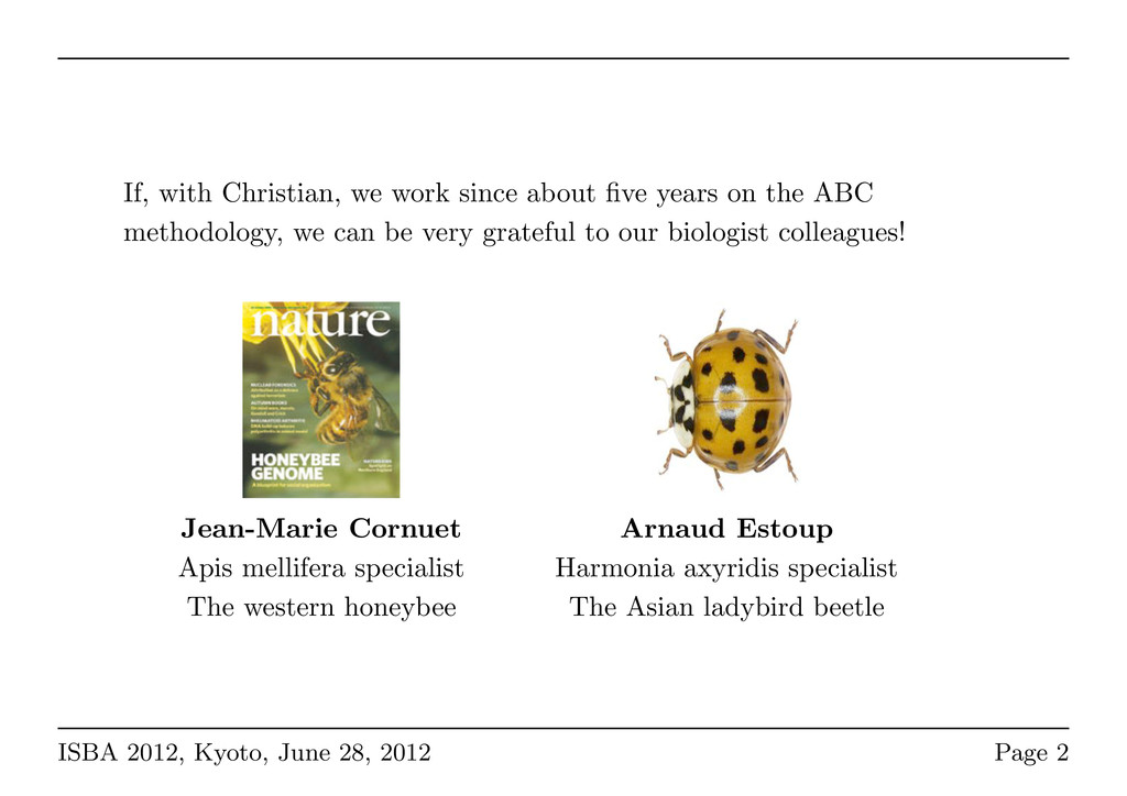
2. If, with Christian, we work since about five years on the ABC methodology, we can be very grateful to our biologist colleagues! Jean-Marie Cornuet Apis mellifera specialist The western honeybee Arnaud Estoup Harmonia axyridis specialist The Asian ladybird beetle ISBA 2012, Kyoto, June 28, 2012 Page 2
3. Arnaud and Jean-Marie typical questions: • How the Asian ladybird beetle arrived in Europe? • Why does they swarm right now? • What are the routes of invasion? • How to get rid of them? Lombaert et al. (2010) PLoS ONE ISBA 2012, Kyoto, June 28, 2012 Page 3
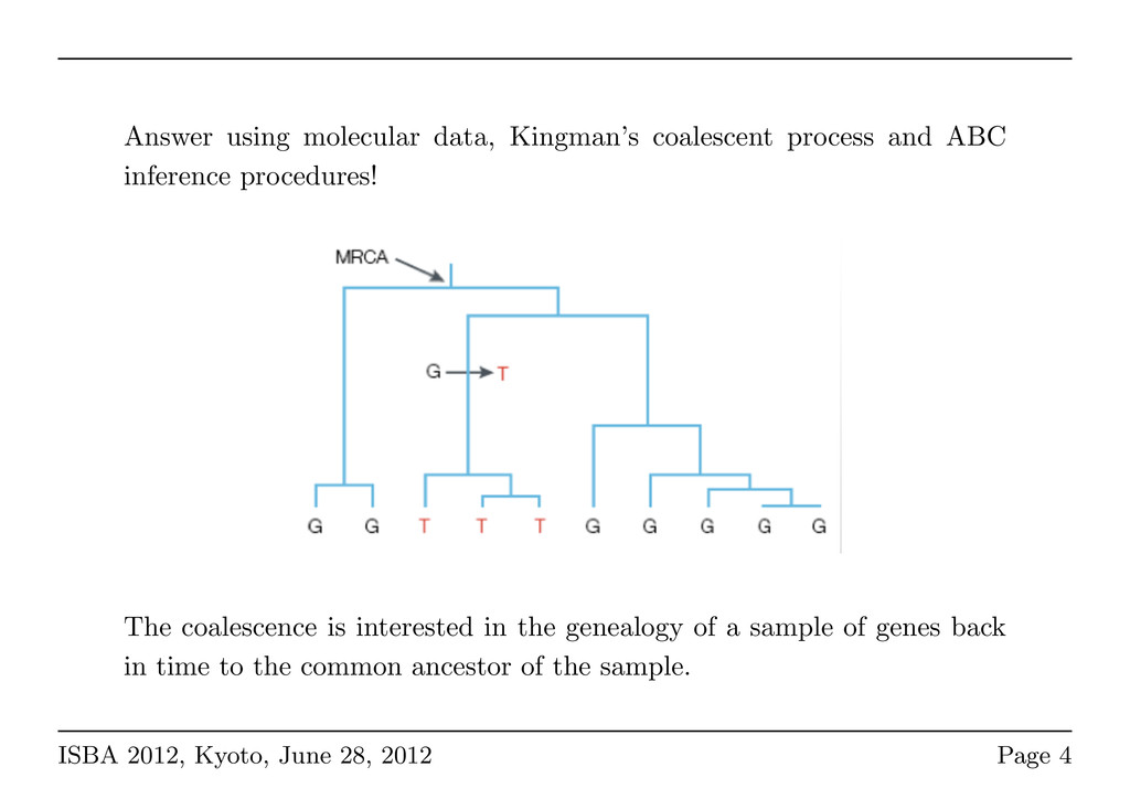
4. Answer using molecular data, Kingman’s coalescent process and ABC inference procedures! Sous l’hypothèse de neutralité des marqueurs gén les mutations sont indépendantes de la généalogie i.e. la généalogie ne dépend que des processus dé On construit donc la généalogie selon les paramètr démographiques (ex. N), puis on ajoute a mutations sur les branches, du MR l’arbre On obtient ainsi d polymorphisme s démographiques considérés The coalescence is interested in the genealogy of a sample of genes back in time to the common ancestor of the sample. ISBA 2012, Kyoto, June 28, 2012 Page 4
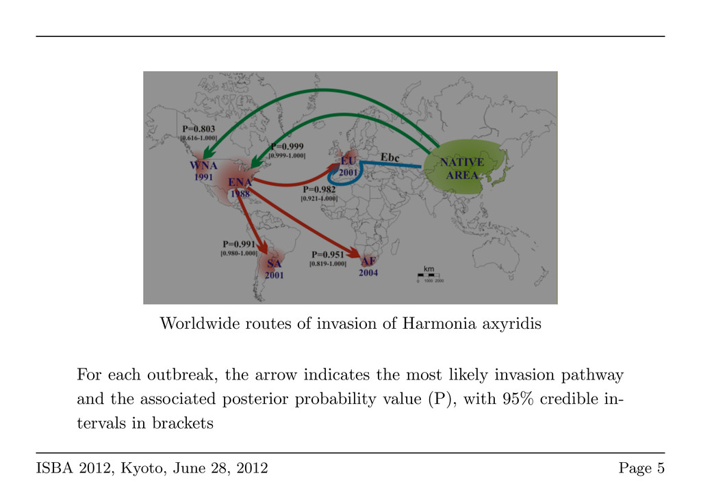
5. Worldwide routes of invasion of Harmonia axyridis For each outbreak, the arrow indicates the most likely invasion pathway and the associated posterior probability value (P), with 95% credible in- tervals in brackets ISBA 2012, Kyoto, June 28, 2012 Page 5
6. ISBA 2012, Kyoto, June 28, 2012 Page 6
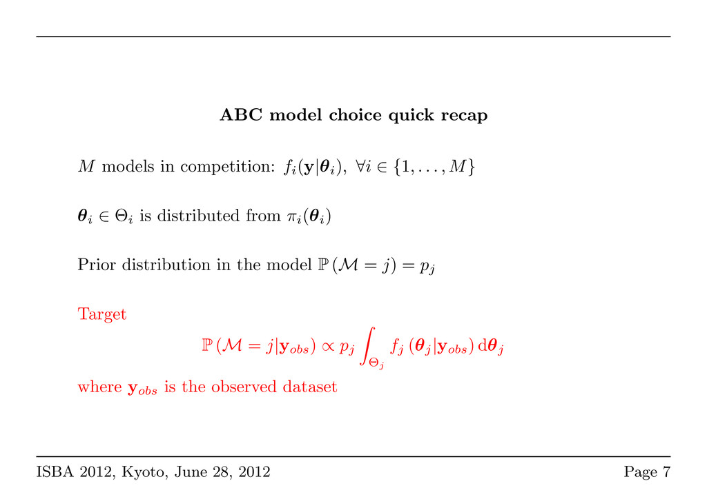
7. ABC model choice quick recap M models in competition: fi (y|θi ), ∀i ∈ {1, . . . , M} θi ∈ Θi is distributed from πi (θi ) Prior distribution in the model P (M = j) = pj Target P (M = j|yobs ) ∝ pj Θj fj (θj |yobs ) dθj where yobs is the observed dataset ISBA 2012, Kyoto, June 28, 2012 Page 7
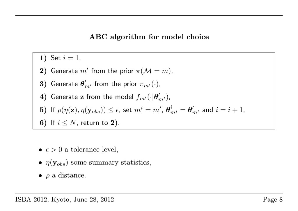
8. ABC algorithm for model choice 1) Set i = 1, 2) Generate m from the prior π(M = m), 3) Generate θm from the prior πm (·), 4) Generate z from the model fm (·|θm ), 5) If ρ(η(z), η(yobs )) ≤ , set mi = m , θi mi = θm and i = i + 1, 6) If i ≤ N, return to 2). • > 0 a tolerance level, • η(yobs ) some summary statistics, • ρ a distance. ISBA 2012, Kyoto, June 28, 2012 Page 8
9. Is that algorithm corresponds to what people really do? No, in practice, they do not have a fixed tolerance level. The tolerance level is a random variable and the number of simulations is fixed! ISBA 2012, Kyoto, June 28, 2012 Page 9
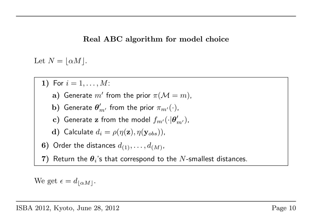
10. Real ABC algorithm for model choice Let N = αM . 1) For i = 1, . . . , M: a) Generate m from the prior π(M = m), b) Generate θm from the prior πm (·), c) Generate z from the model fm (·|θm ), d) Calculate di = ρ(η(z), η(yobs )), 6) Order the distances d(1) , . . . , d(M) , 7) Return the θi ’s that correspond to the N-smallest distances. We get = d αM . ISBA 2012, Kyoto, June 28, 2012 Page 10
11. Lack of confidence in approximate Bayesian computation model choice (Robert, Cornuet, Marin and Pillai (2011) PNAS) There is a fundamental discrepancy between the genuine Bayes fac- tors/posterior probabilities and the approximations resulting from ABC model choice. Use of insufficient statistics can be a real difficulty for model choice! ISBA 2012, Kyoto, June 28, 2012 Page 11
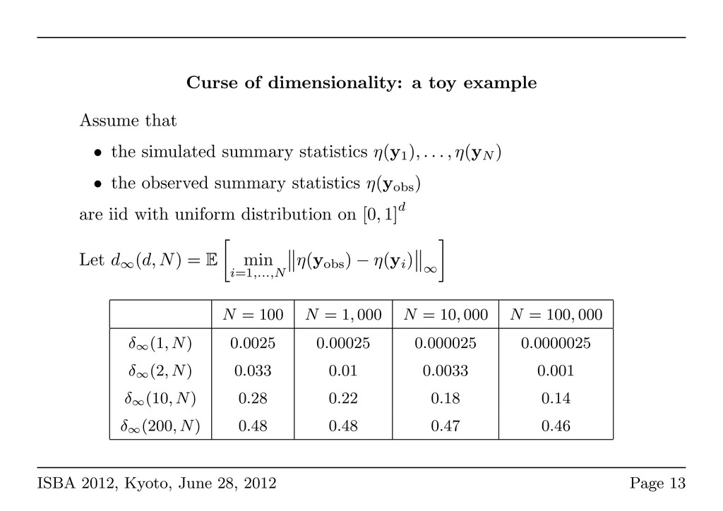
12. Relevant statistics for Bayesian model choice (Marin, Pillai, Robert, Rousseau (2012)) We derive necessary and sufficient conditions on summary statistics for the corresponding Bayes factor to be convergent, namely to asymptotically select the true model. The assumption can be checked for summary statistics of empirical type (we study the case of the δµ2 distances for population genetics models). More generally, you should keep the maximum information from the data. But if the dimension of the summary statistics is too large: curse of dimensionality. ISBA 2012, Kyoto, June 28, 2012 Page 12
13. Curse of dimensionality: a toy example Assume that • the simulated summary statistics η(y1 ), . . . , η(yN ) • the observed summary statistics η(yobs ) are iid with uniform distribution on [0, 1]d Let d∞ (d, N) = E min i=1,...,N η(yobs ) − η(yi ) ∞ N = 100 N = 1, 000 N = 10, 000 N = 100, 000 δ∞ (1, N) 0.0025 0.00025 0.000025 0.0000025 δ∞ (2, N) 0.033 0.01 0.0033 0.001 δ∞ (10, N) 0.28 0.22 0.18 0.14 δ∞ (200, N) 0.48 0.48 0.47 0.46 ISBA 2012, Kyoto, June 28, 2012 Page 13
14. Types I and II errors In practice, people produce Type I and II errors validation of their ABC model choice procedure. Type I error: exclude scenario x when it is actually scenario x Type II error: choose scenario x when it is not scenario x That validation, done for each scenario, can be computationally inten- sive if the number of summary statistics is large. ISBA 2012, Kyoto, June 28, 2012 Page 14
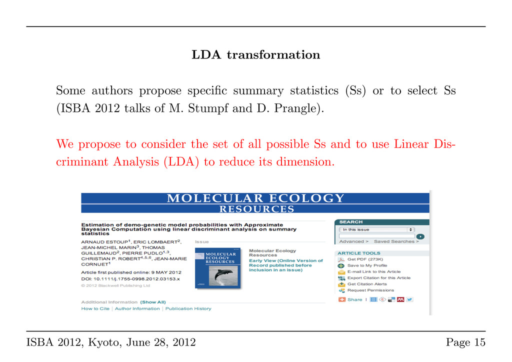
15. LDA transformation Some authors propose specific summary statistics (Ss) or to select Ss (ISBA 2012 talks of M. Stumpf and D. Prangle). We propose to consider the set of all possible Ss and to use Linear Dis- criminant Analysis (LDA) to reduce its dimension. ISBA 2012, Kyoto, June 28, 2012 Page 15
16. Our methodology Step 1: We selected a subset of x% (typically 1%) best sim- ulations in a standard ABC reference table usually including 106 simulations for each of the M compared scenarios. This selection was based on the standard normalized Euclidian distance computed between the observed and simulated raw (not transformed) Ss. Step 2 (LDA step): we used LDA to transform the raw Ss of this subset of x% best simulations into (M−1) discriminant variables. When computing LDA functions, we weighted the simulated data sets with the Epanechnikov kernel commonly used in the local regression. ISBA 2012, Kyoto, June 28, 2012 Page 16
17. Step 3: We estimated the posterior probabilities of each compet- ing scenario by polychotomous local logistic regression (Cornuet et al. (2008) Bioinformatics) on the x% best simulated data sets now summarized by M − 1 discriminant variables. ISBA 2012, Kyoto, June 28, 2012 Page 17
18. Processing Step 2 provides three main advantages: • computation of scenario probabilities using the polychotomous regres- sion of Step 3 becomes much faster; • a lower number of explanatory variables may improve the accuracy of the ABC approximation, particularly when the number of simulations is not large enough to offset the number of Ss; • using LDA-transformed Ss avoids correlations among explanatory variables. ISBA 2012, Kyoto, June 28, 2012 Page 18
19. We show, using both simulated and real data sets, that posterior prob- abilities of scenarios computed from LDA-transformed and raw Ss are strongly correlated. Faster probability computation increases the ability of ABC practitioners to analyze large numbers of pseudo-observations data sets to evaluate Type I and II errors. We believe that our LDA-based proposal will usefully enlarge the tool box available to biologists to make ABC inferences on more complex and hence more realistic demographic processes. ISBA 2012, Kyoto, June 28, 2012 Page 19