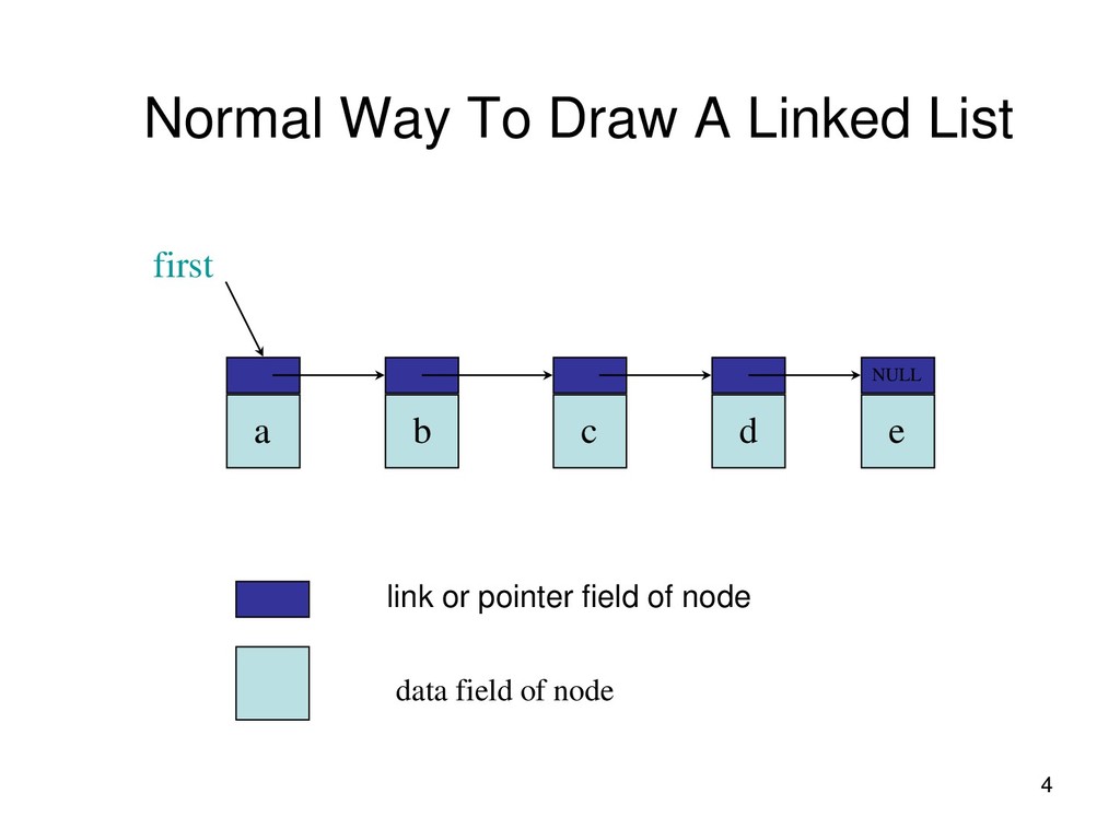
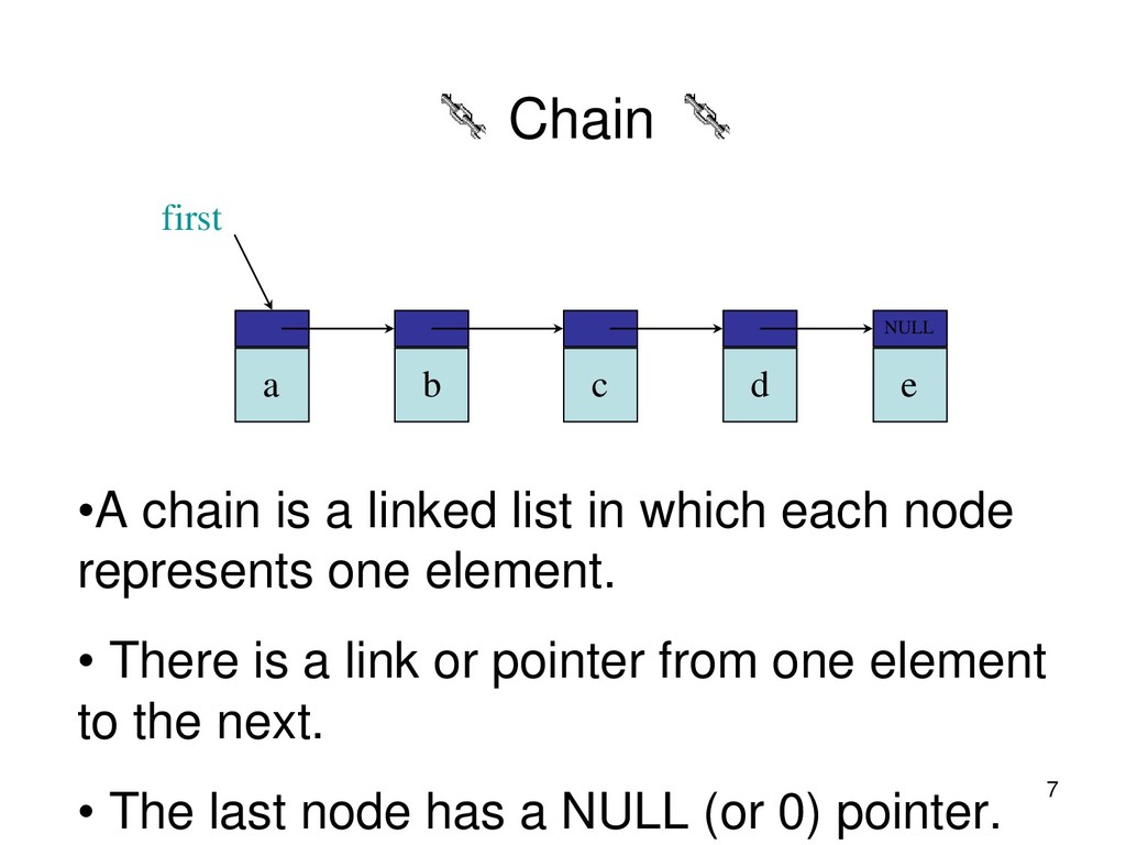
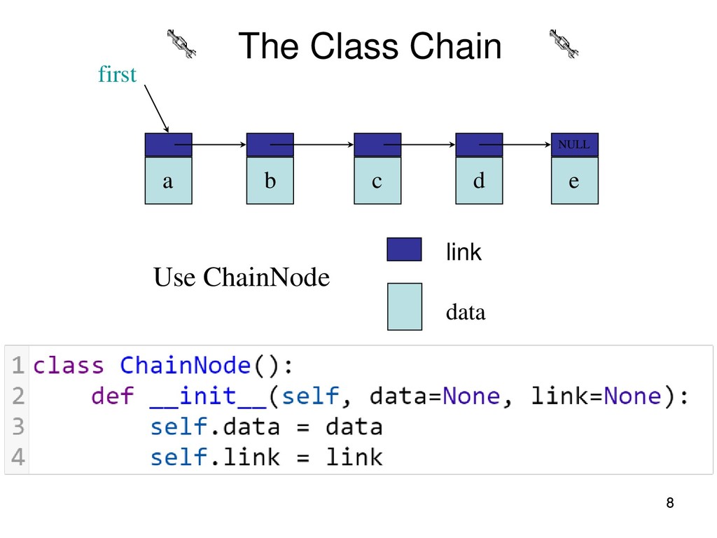
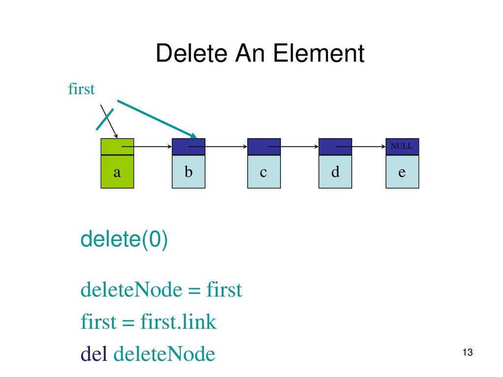
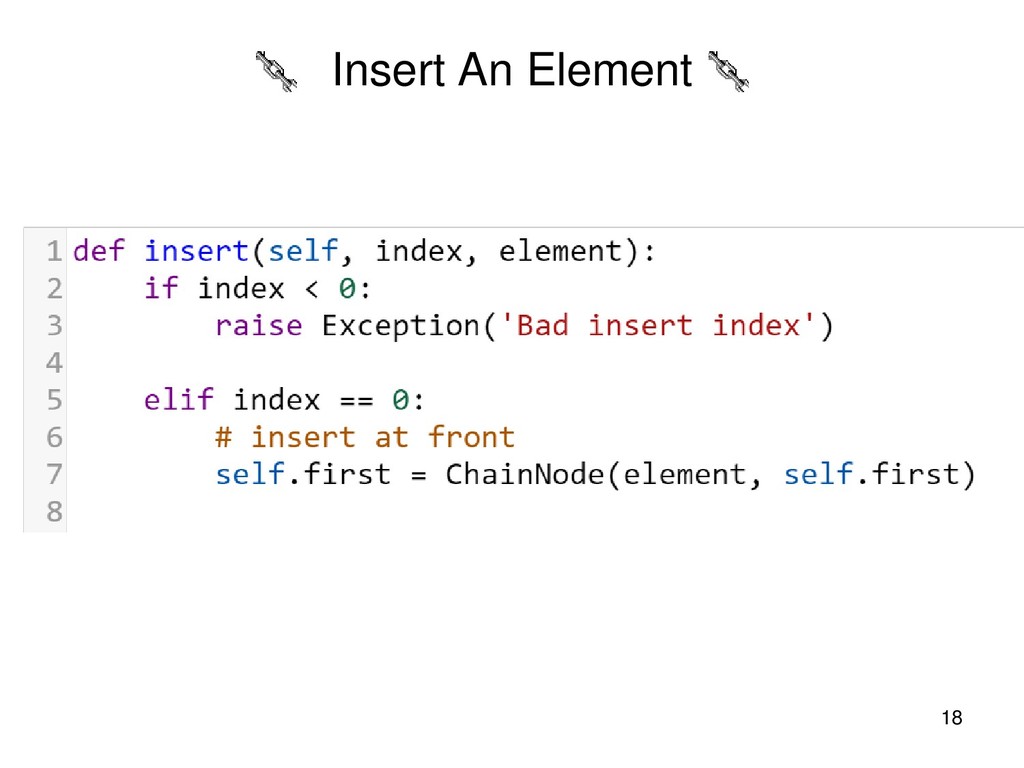
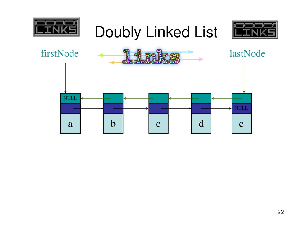
each node represents one element. • There is a link or pointer from one element to the next. • The last node has a NULL (or 0) pointer. a b c d e NULL first
Tree • What it can be used for ? An example • Postfix, Infix, Prefix • Full binary Tree and Complete Binary tree • How to keep the tree data in array or linked list 26
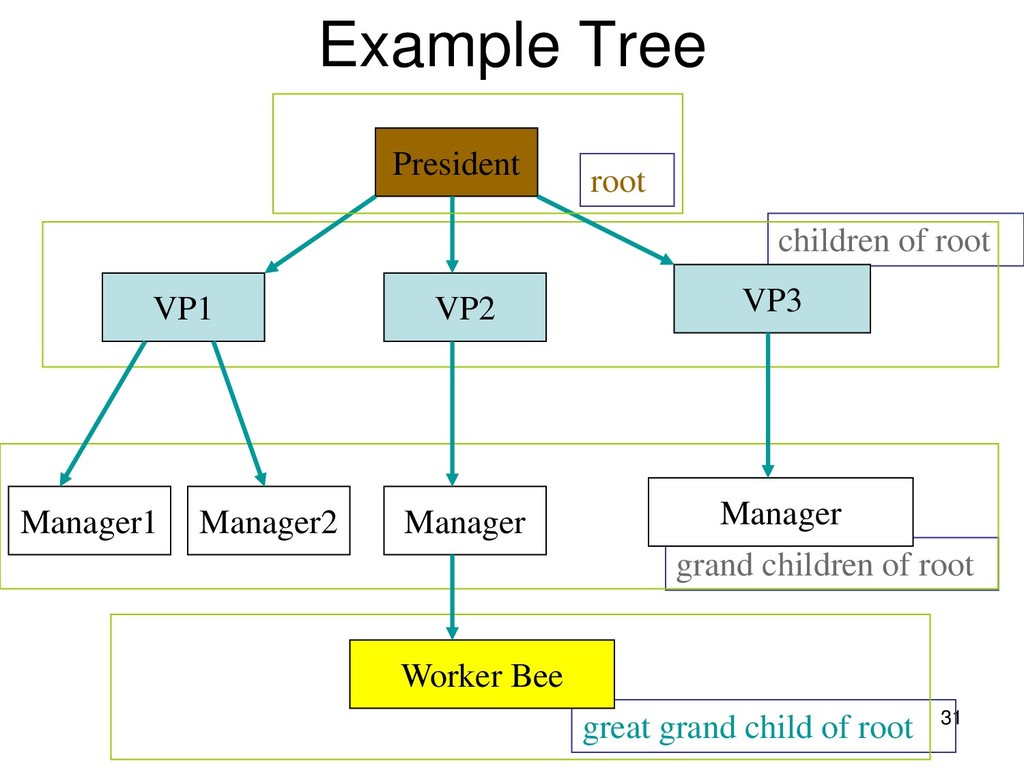
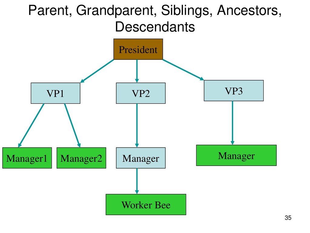
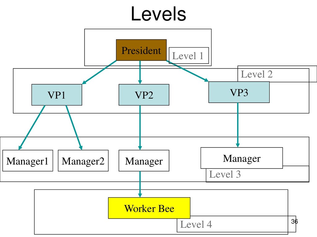
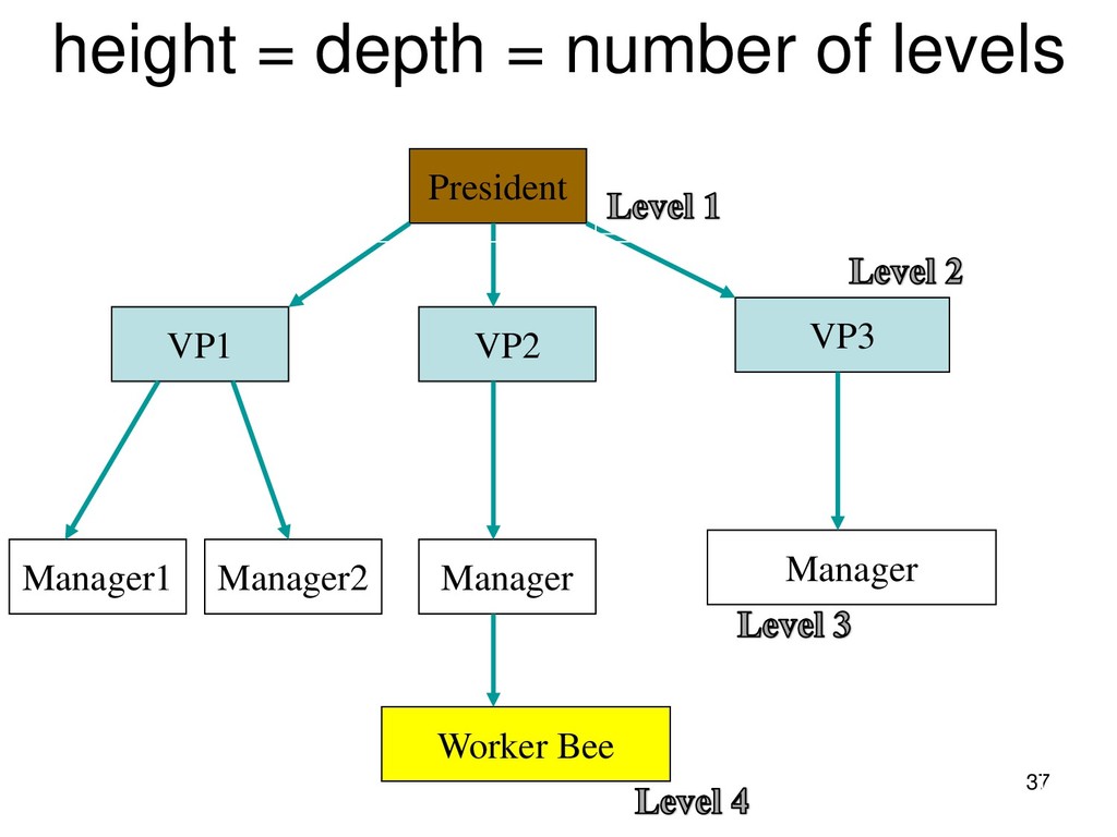
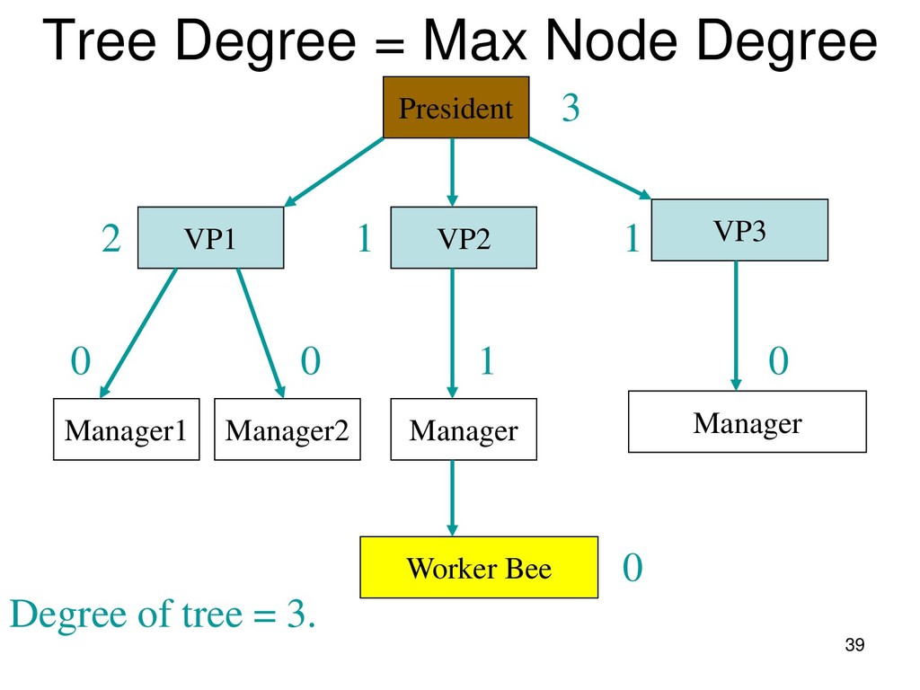
for serially ordered data. – (e0 , e1 , e2 , …, en-1 ) – Days of week. – Months in a year. – Students in this class. • Trees are useful for hierarchically ordered data. – Employees of a corporation. • President, vice presidents, managers, and so on.
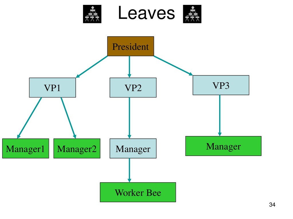
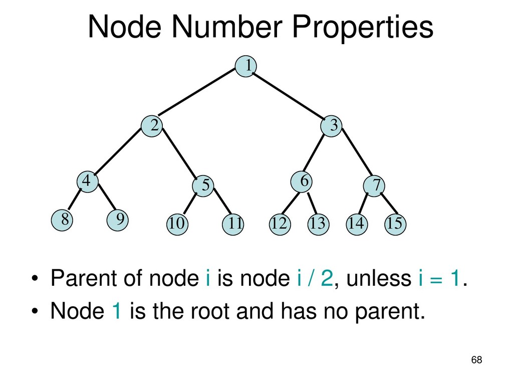
top of the hierarchy is the root. • Elements next in the hierarchy are the children of the root. • Elements next in the hierarchy are the grandchildren of the root, and so on. • Elements that have no children are leaves.
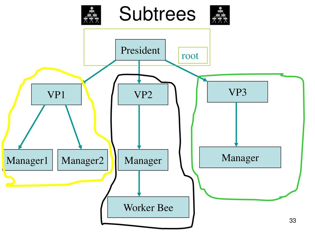
set of elements. • One of these elements is called the root. • The remaining elements, if any, are partitioned into trees, which are called the subtrees of t.
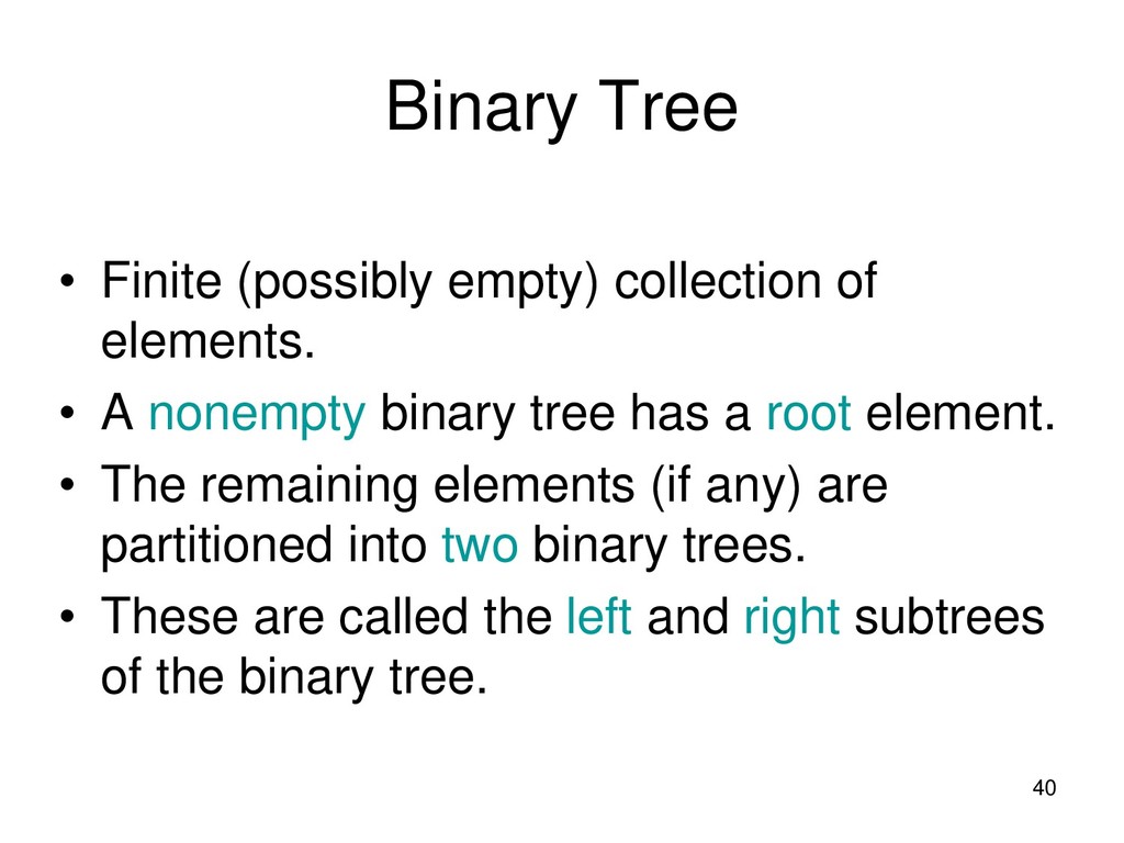
• A nonempty binary tree has a root element. • The remaining elements (if any) are partitioned into two binary trees. • These are called the left and right subtrees of the binary tree.
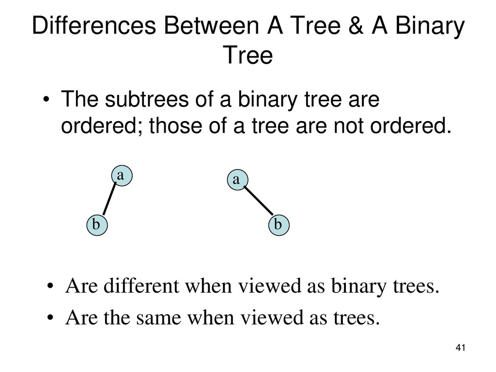
The subtrees of a binary tree are ordered; those of a tree are not ordered. a b a b • Are different when viewed as binary trees. • Are the same when viewed as trees.
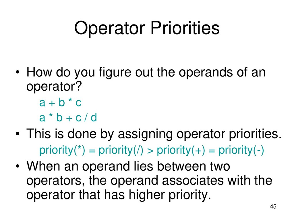
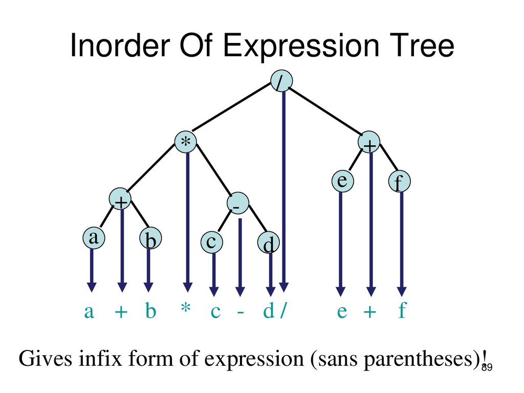
operands of an operator? – a + b * c – a * b + c / d • This is done by assigning operator priorities. – priority(*) = priority(/) > priority(+) = priority(-) • When an operand lies between two operators, the operand associates with the operator that has higher priority.
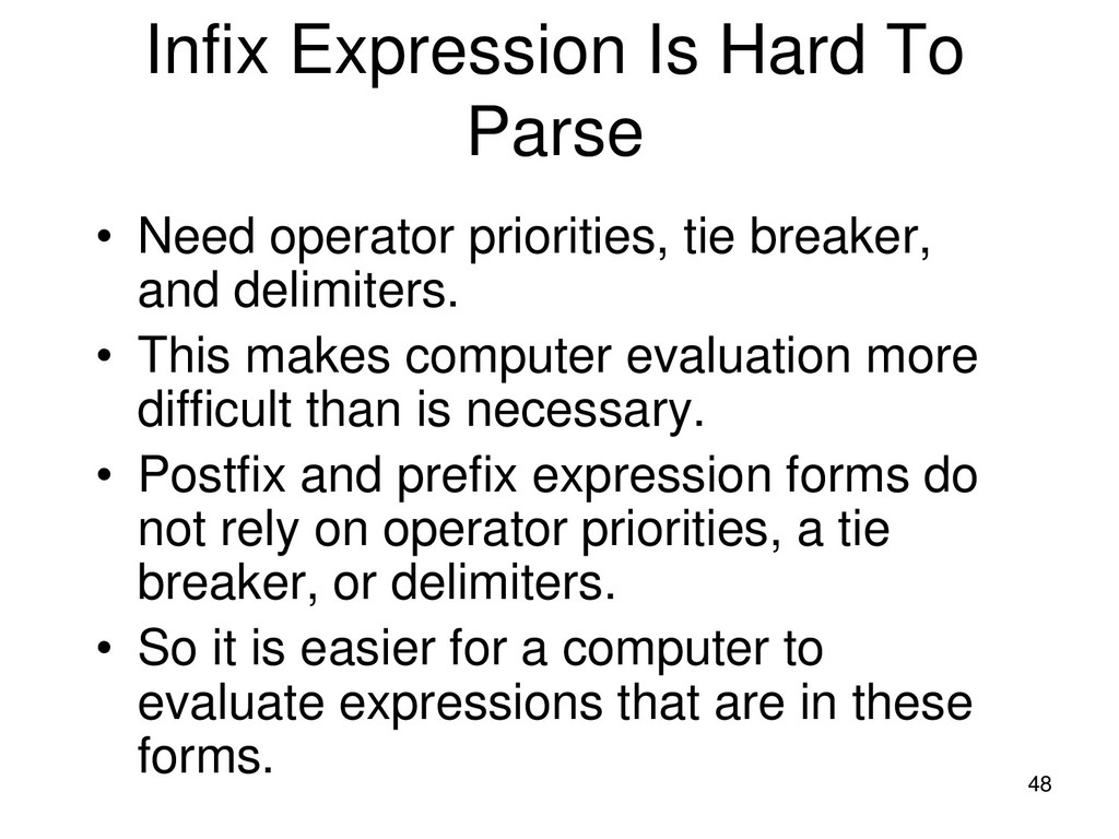
priorities, tie breaker, and delimiters. • This makes computer evaluation more difficult than is necessary. • Postfix and prefix expression forms do not rely on operator priorities, a tie breaker, or delimiters. • So it is easier for a computer to evaluate expressions that are in these forms.
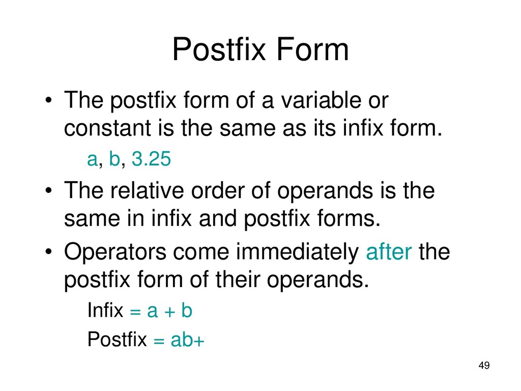
or constant is the same as its infix form. – a, b, 3.25 • The relative order of operands is the same in infix and postfix forms. • Operators come immediately after the postfix form of their operands. – Infix = a + b – Postfix = ab+
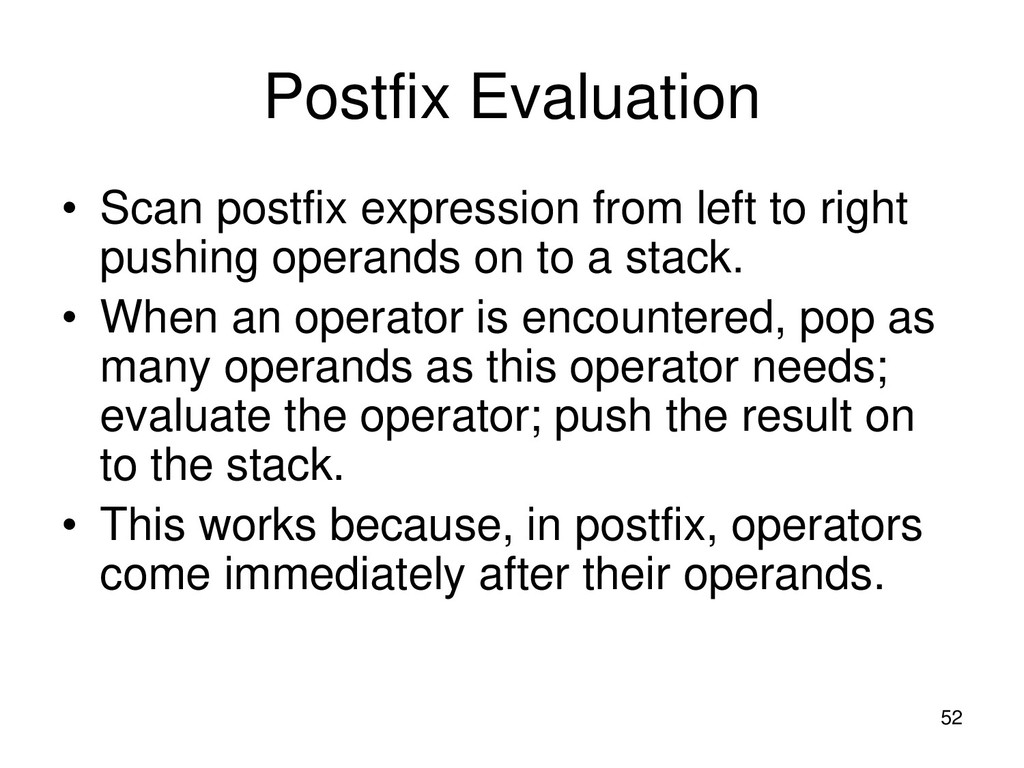
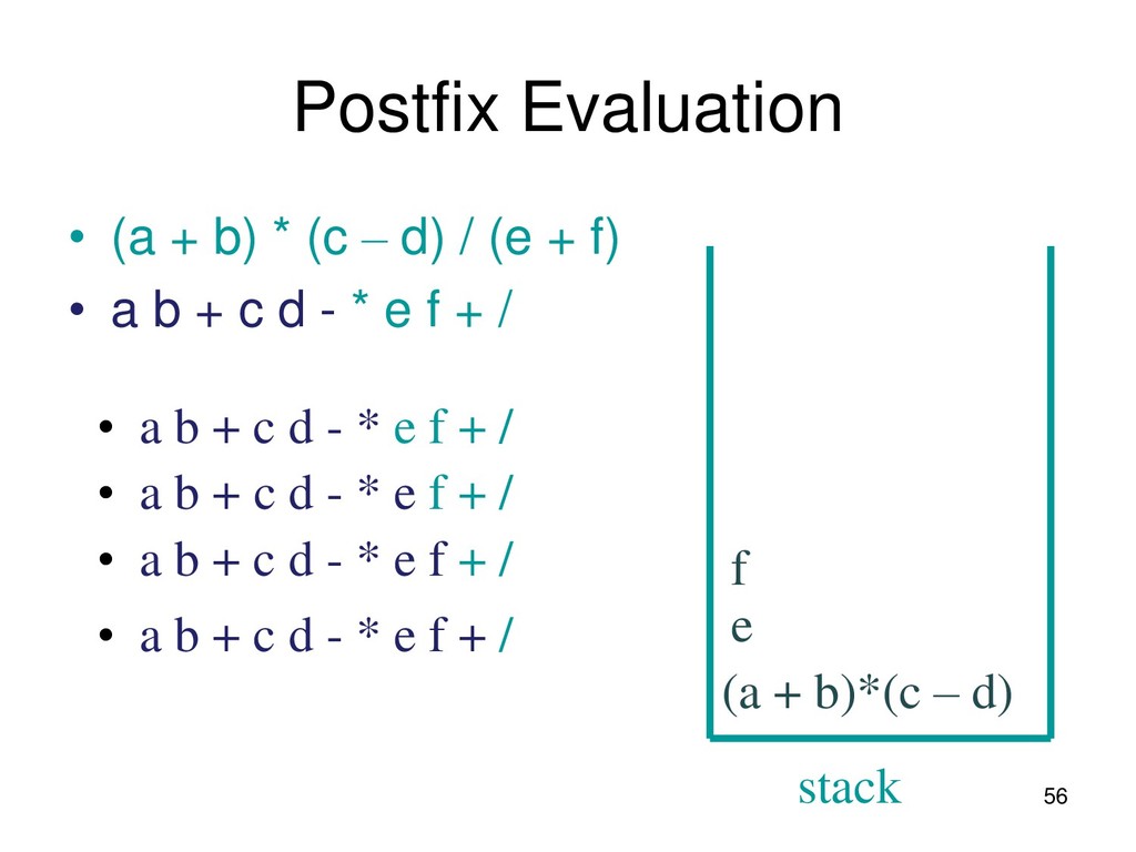
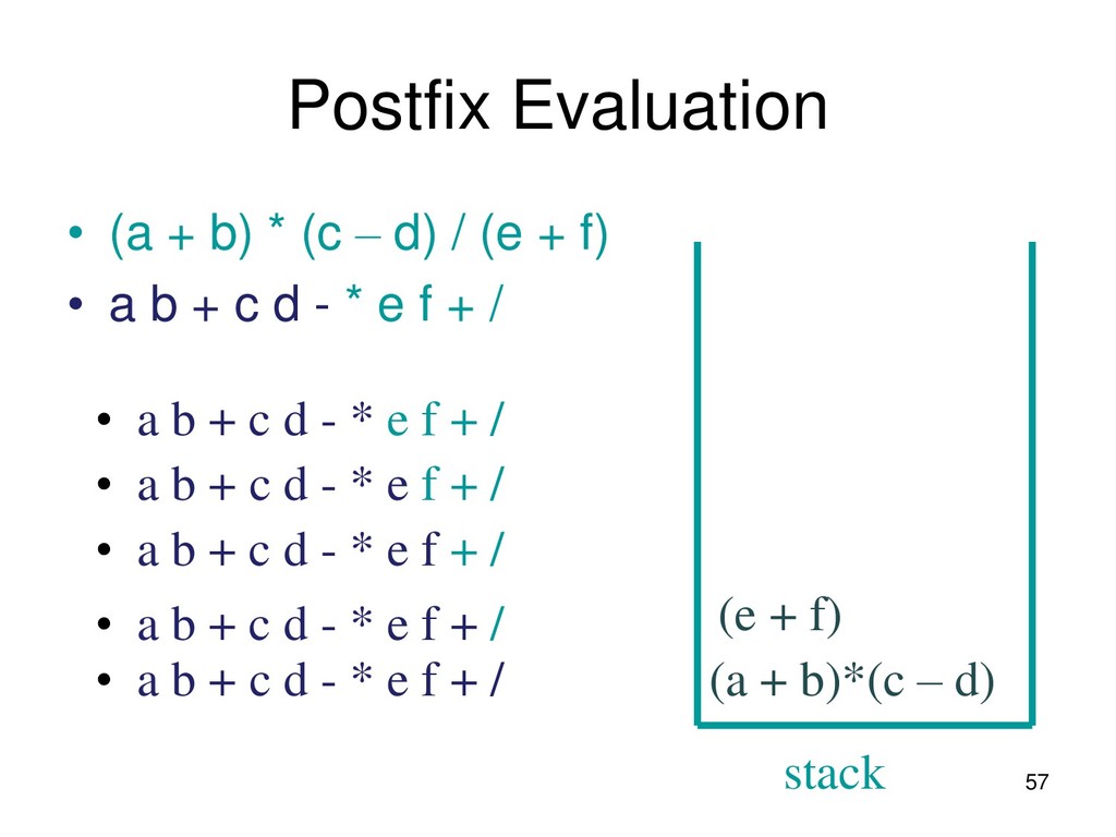
right pushing operands on to a stack. • When an operator is encountered, pop as many operands as this operator needs; evaluate the operator; push the result on to the stack. • This works because, in postfix, operators come immediately after their operands.
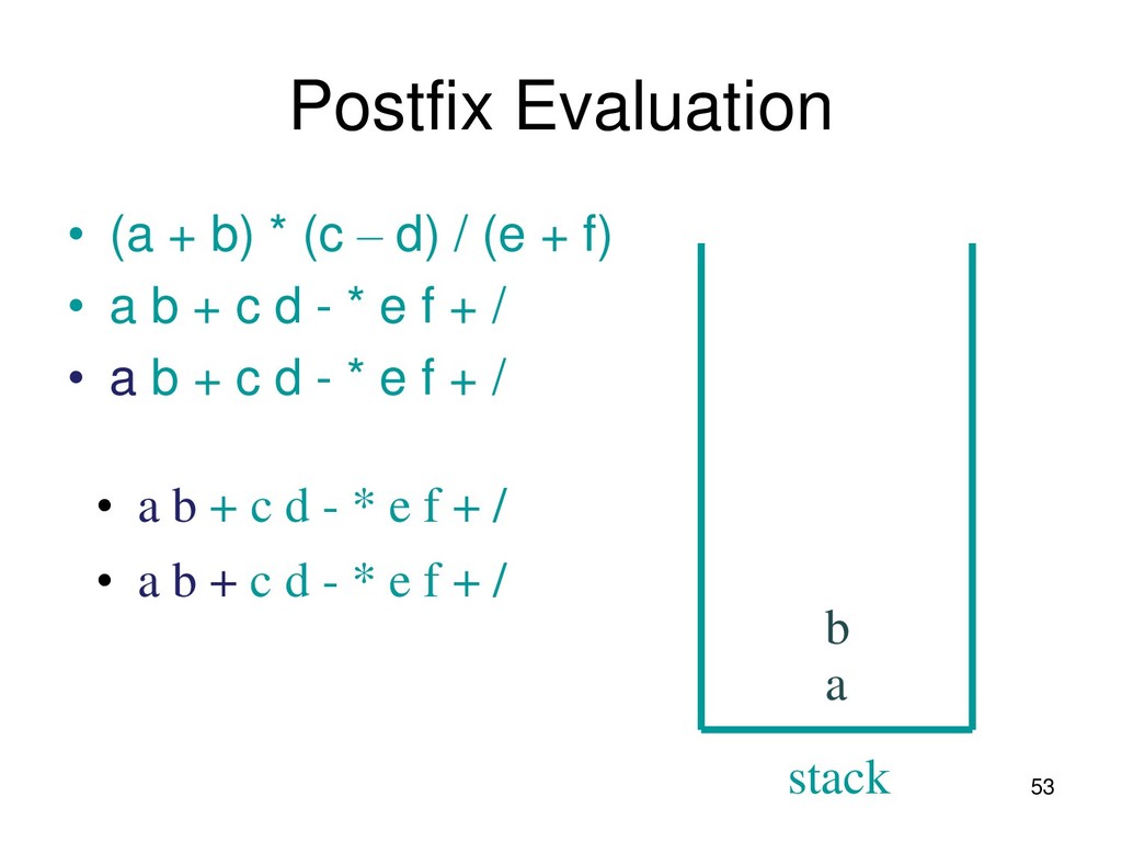
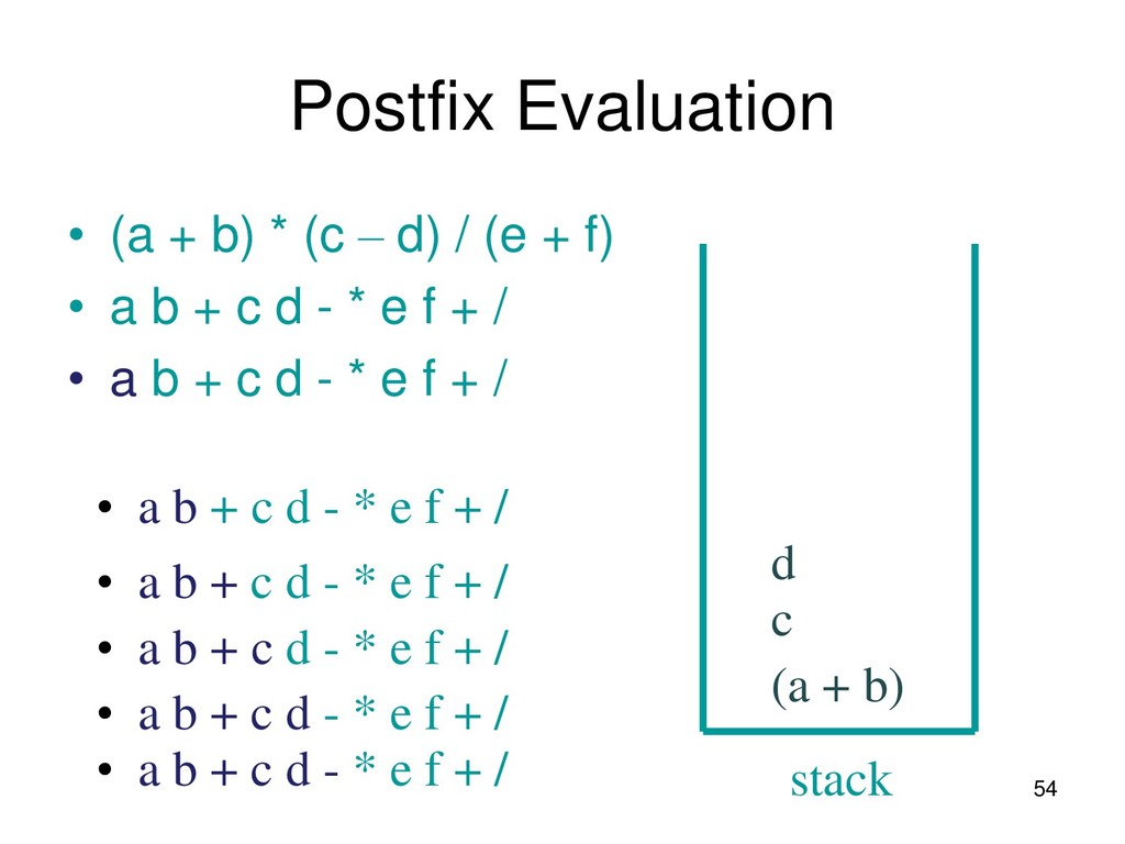
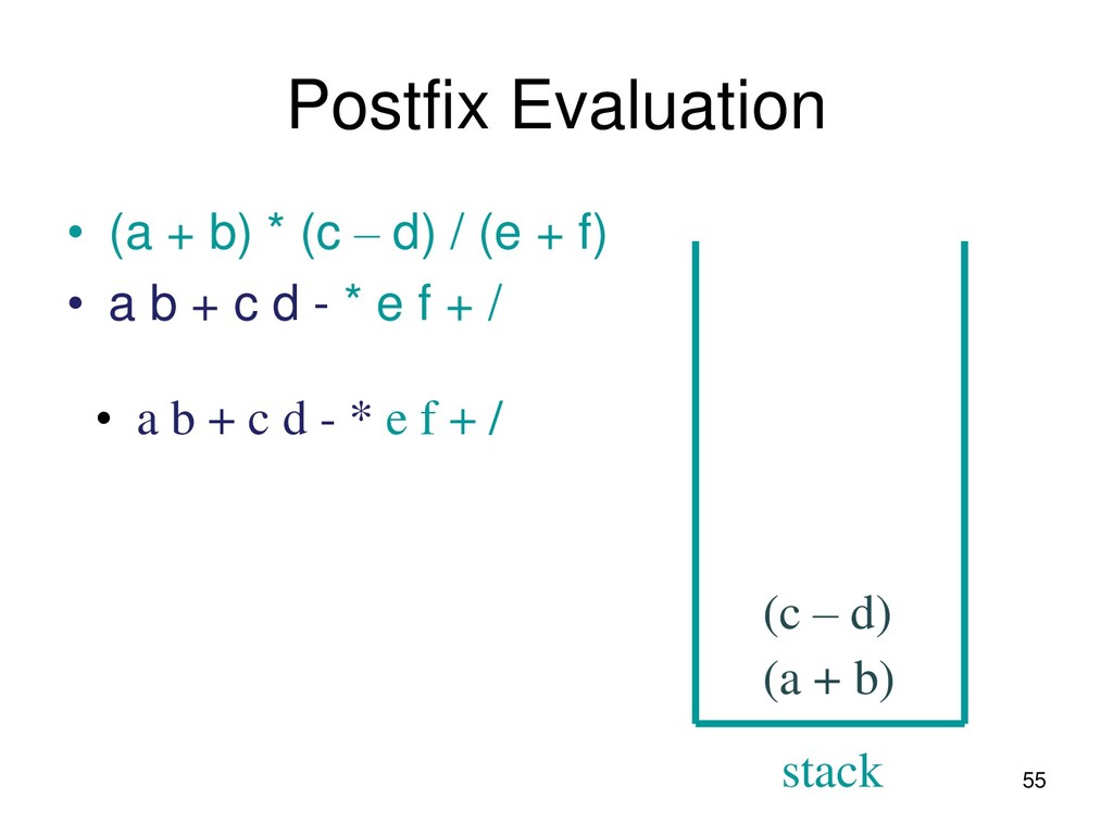
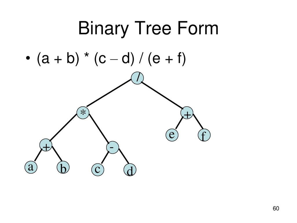
d) / (e + f) • a b + c d - * e f + / • a b + c d - * e f + / stack (a + b) • a b + c d - * e f + / • a b + c d - * e f + / • a b + c d - * e f + / c • a b + c d - * e f + / d • a b + c d - * e f + /
d) / (e + f) • a b + c d - * e f + / stack (a + b)*(c – d) • a b + c d - * e f + / e • a b + c d - * e f + / • a b + c d - * e f + / f • a b + c d - * e f + /
d) / (e + f) • a b + c d - * e f + / stack (a + b)*(c – d) • a b + c d - * e f + / (e + f) • a b + c d - * e f + / • a b + c d - * e f + / • a b + c d - * e f + / • a b + c d - * e f + /
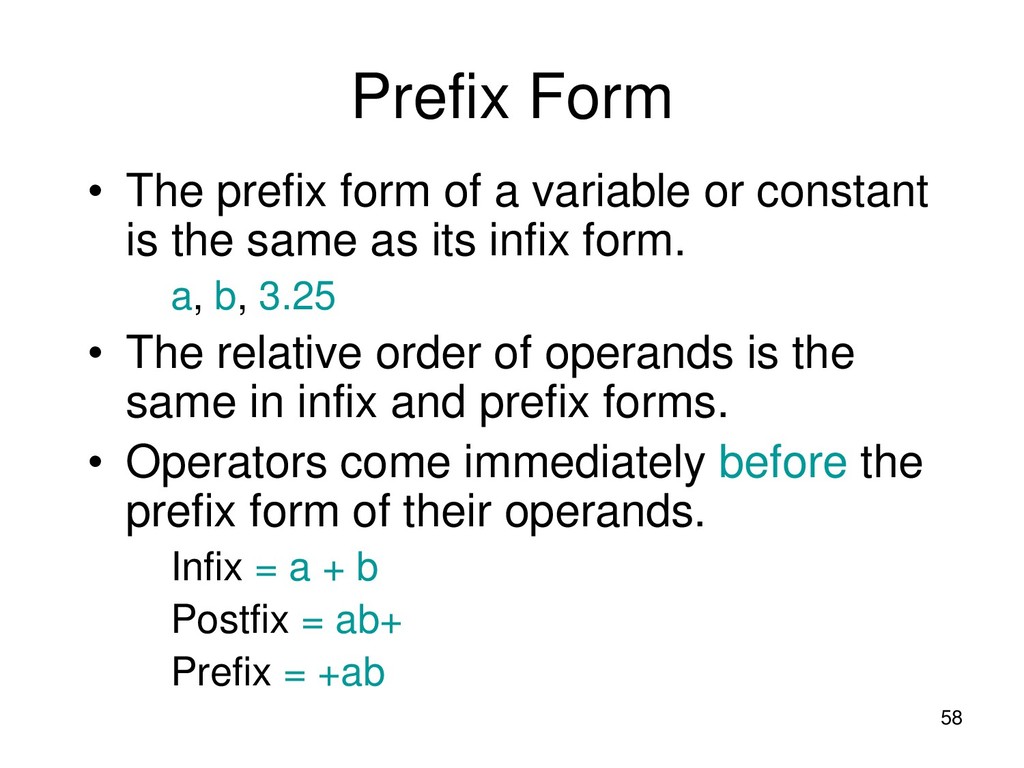
or constant is the same as its infix form. – a, b, 3.25 • The relative order of operands is the same in infix and prefix forms. • Operators come immediately before the prefix form of their operands. – Infix = a + b – Postfix = ab+ – Prefix = +ab
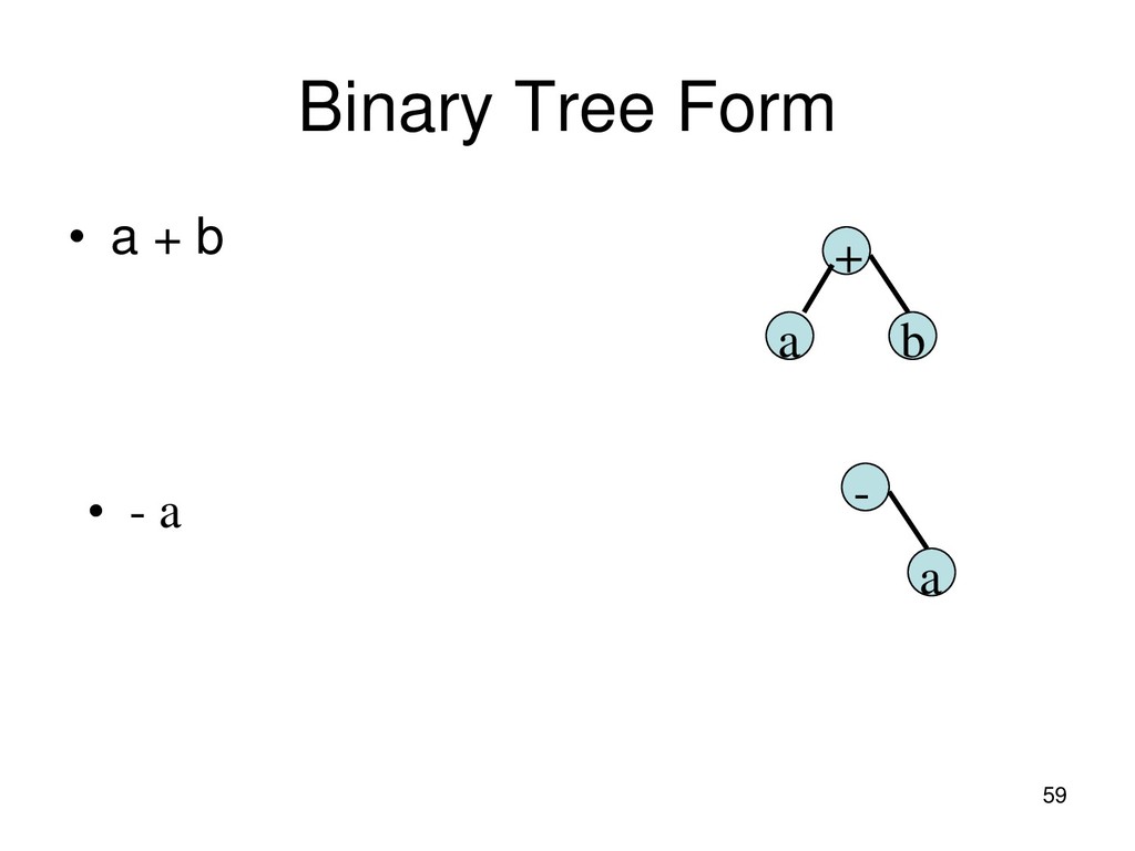
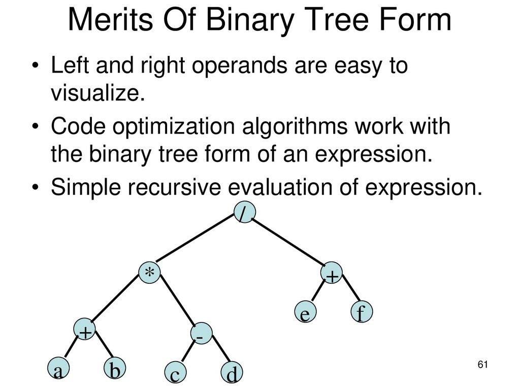
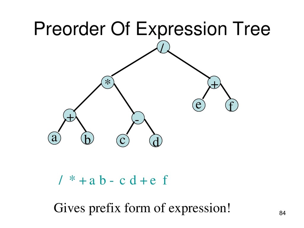
operands are easy to visualize. • Code optimization algorithms work with the binary tree form of an expression. • Simple recursive evaluation of expression. + a b - c d + e f * /
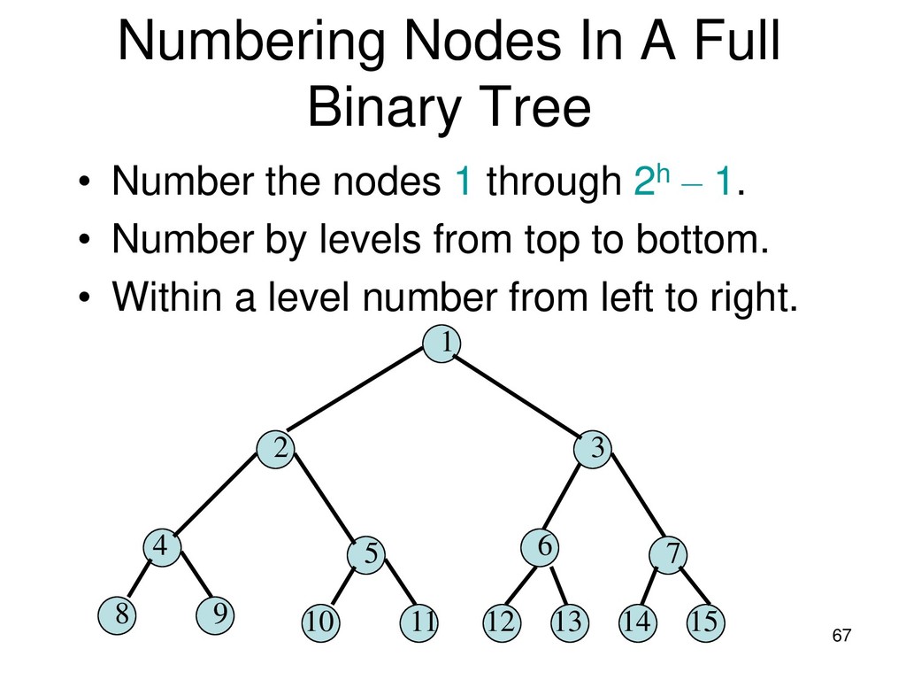
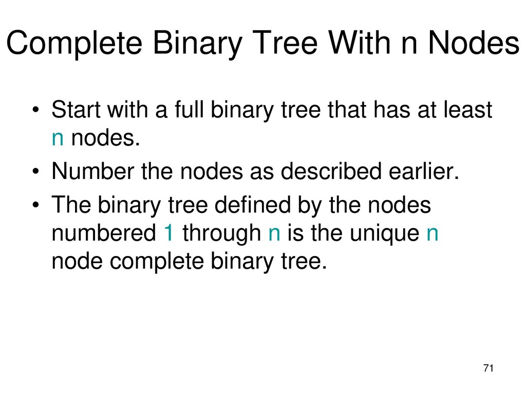
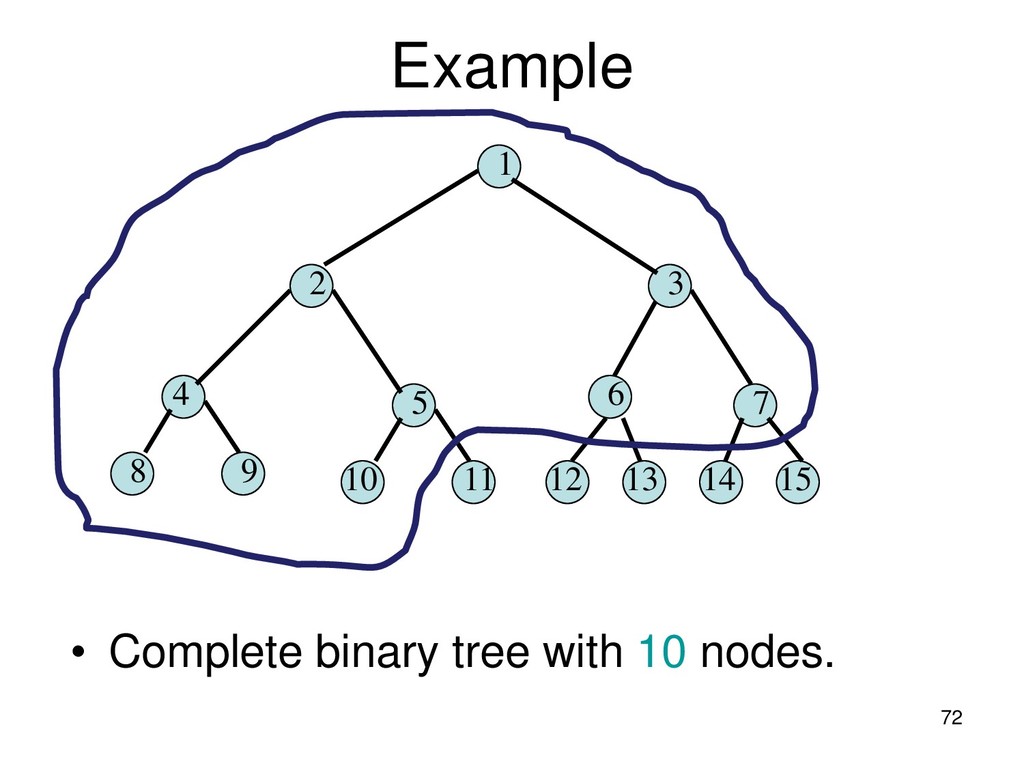
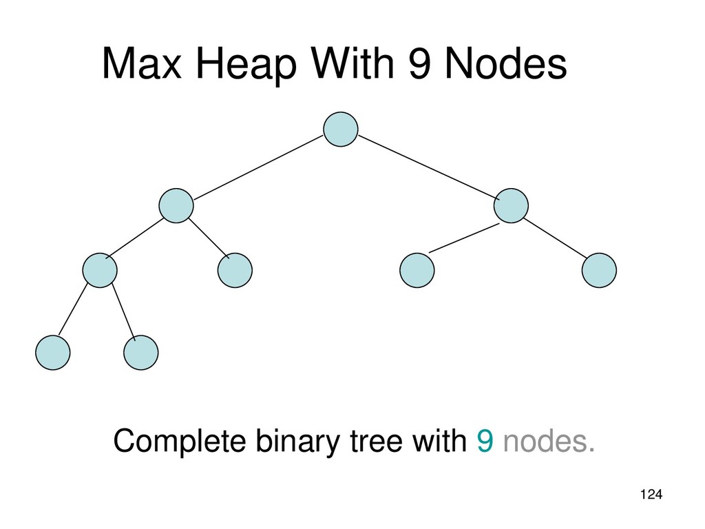
a full binary tree that has at least n nodes. • Number the nodes as described earlier. • The binary tree defined by the nodes numbered 1 through n is the unique n node complete binary tree.
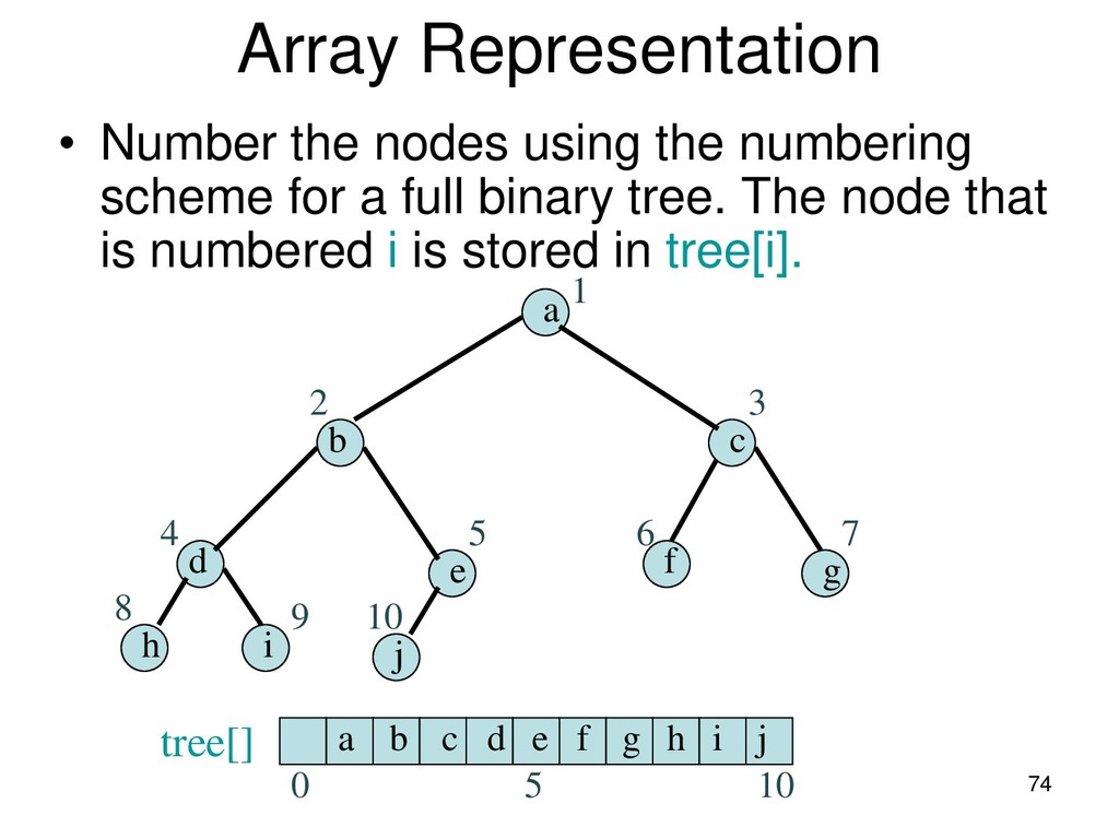
scheme for a full binary tree. The node that is numbered i is stored in tree[i]. tree[] 0 5 10 a b c d e f g h i j b a c d e f g h i j 1 2 3 4 5 6 7 8 9 10
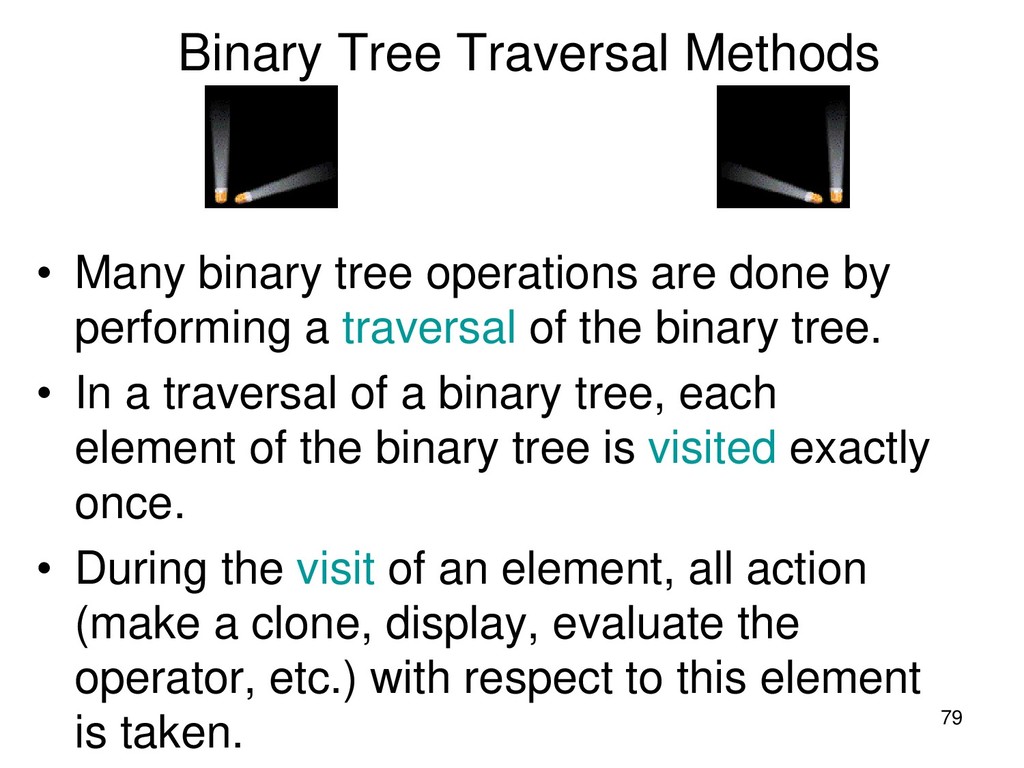
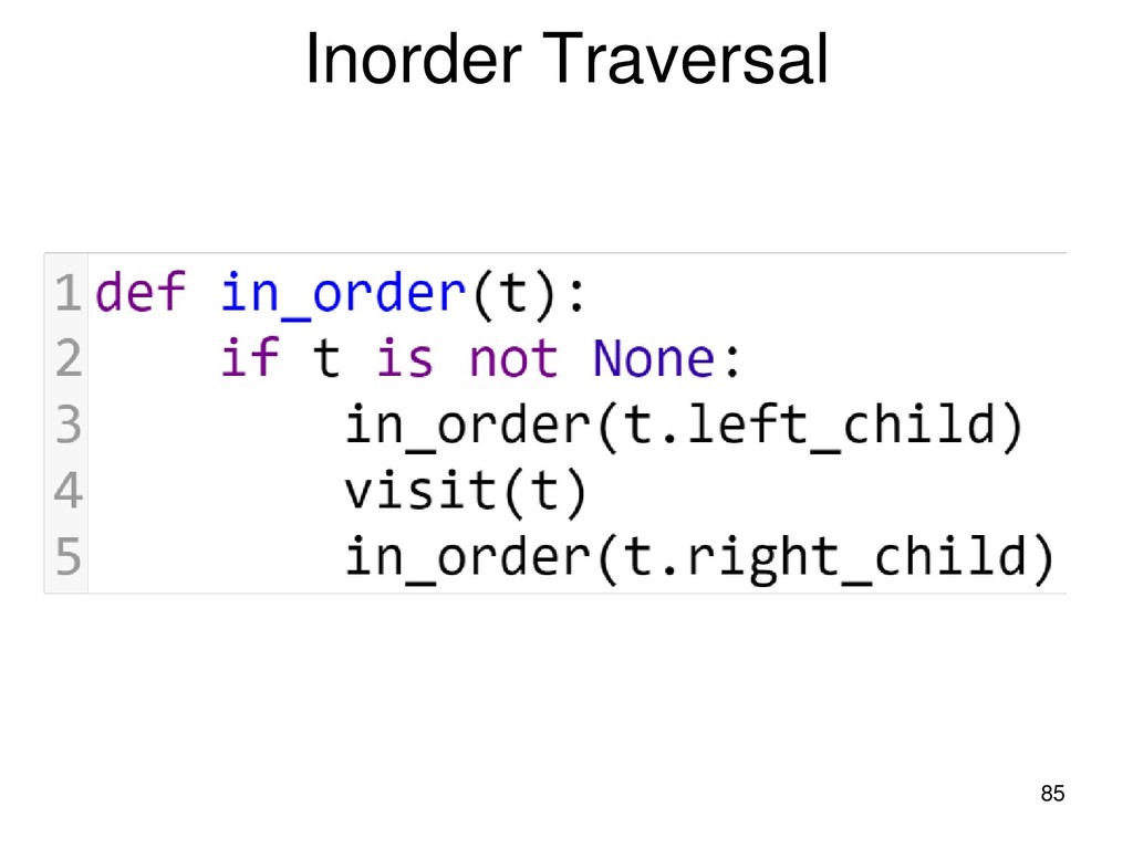
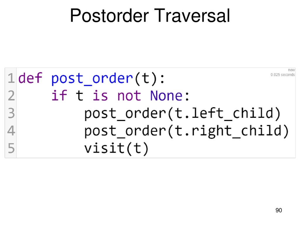
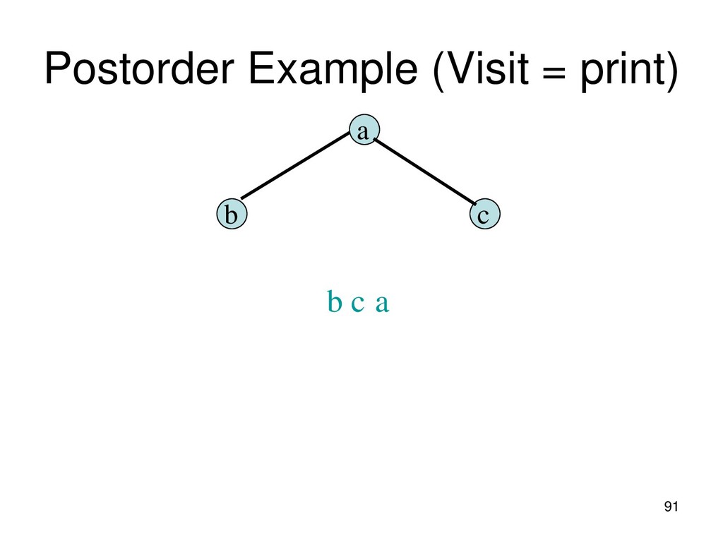
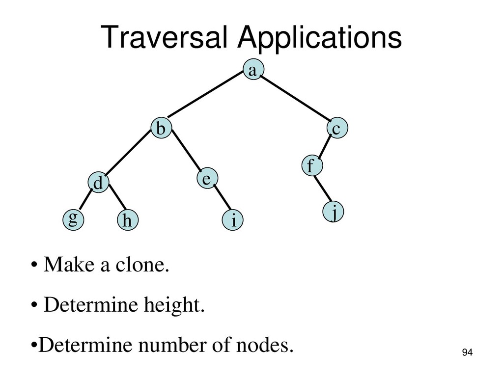
are done by performing a traversal of the binary tree. • In a traversal of a binary tree, each element of the binary tree is visited exactly once. • During the visit of an element, all action (make a clone, display, evaluate the operator, etc.) with respect to this element is taken.
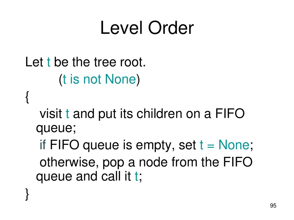
(t is not None) { visit t and put its children on a FIFO queue; if FIFO queue is empty, set t = None; otherwise, pop a node from the FIFO queue and call it t; }
a binary tree are distinct. • Can you construct the binary tree from which a given traversal sequence came? • When a traversal sequence has more than one element, the binary tree is not uniquely defined. • Therefore, the tree from which the sequence was obtained cannot be reconstructed uniquely.
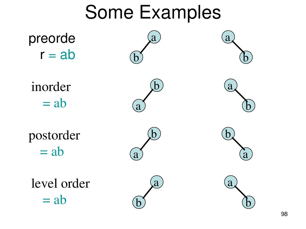
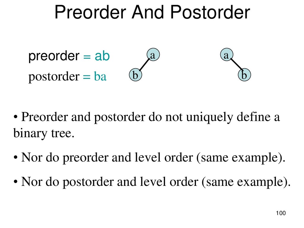
b postorder = ba • Preorder and postorder do not uniquely define a binary tree. • Nor do preorder and level order (same example). • Nor do postorder and level order (same example).
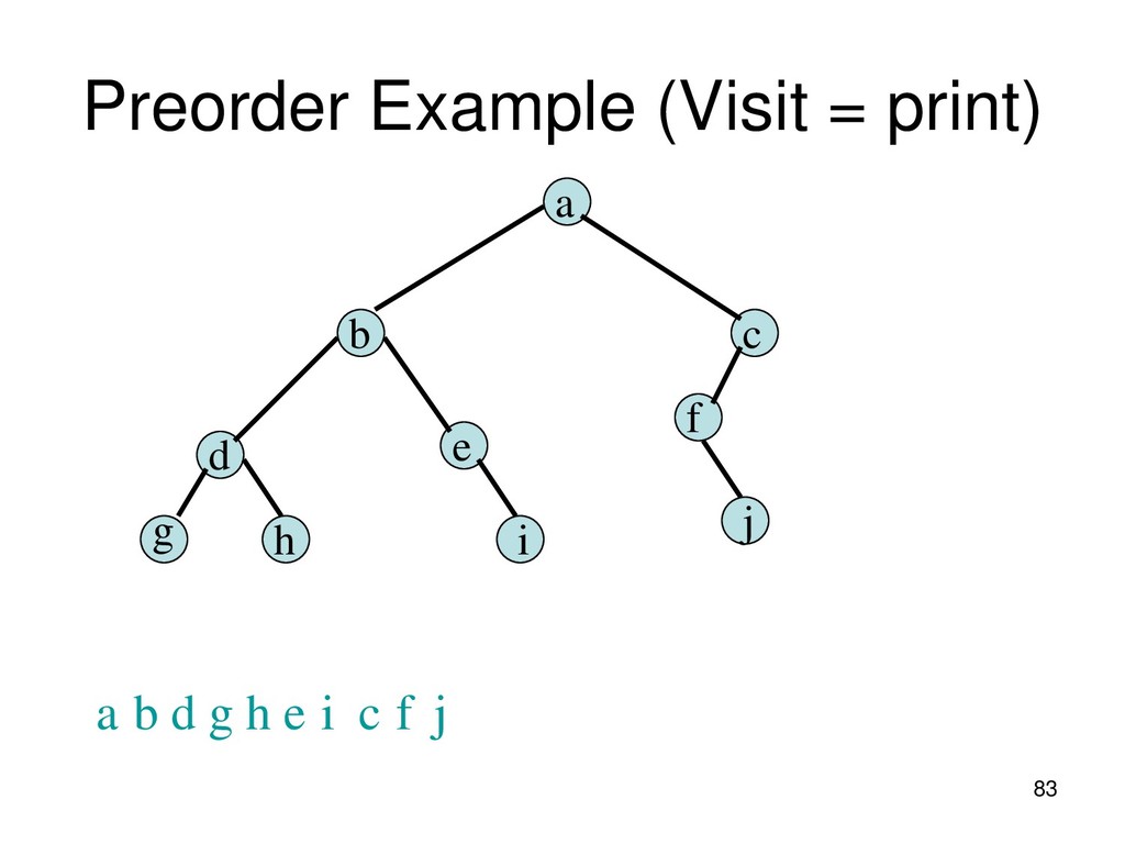
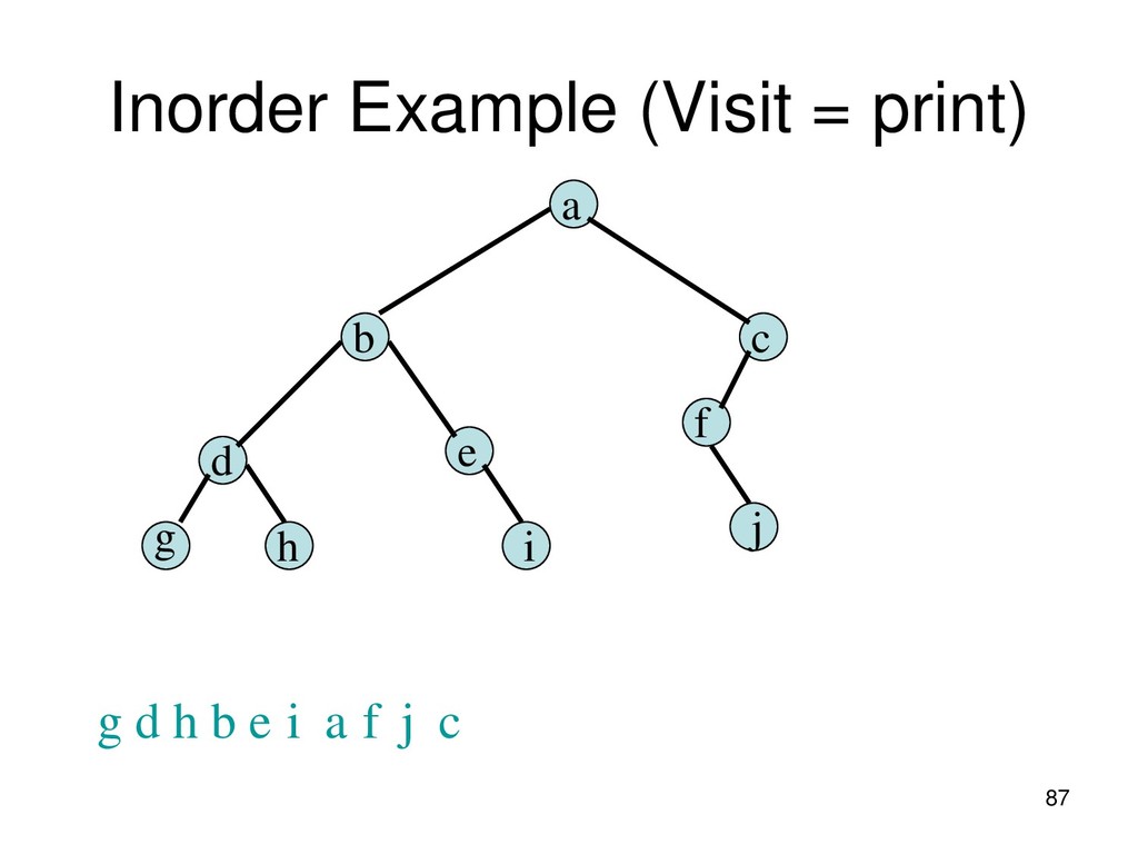
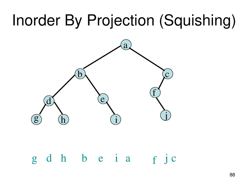
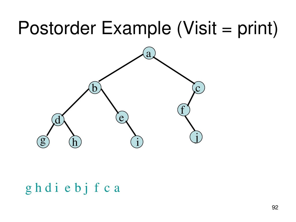
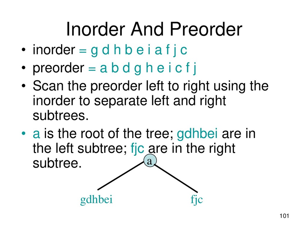
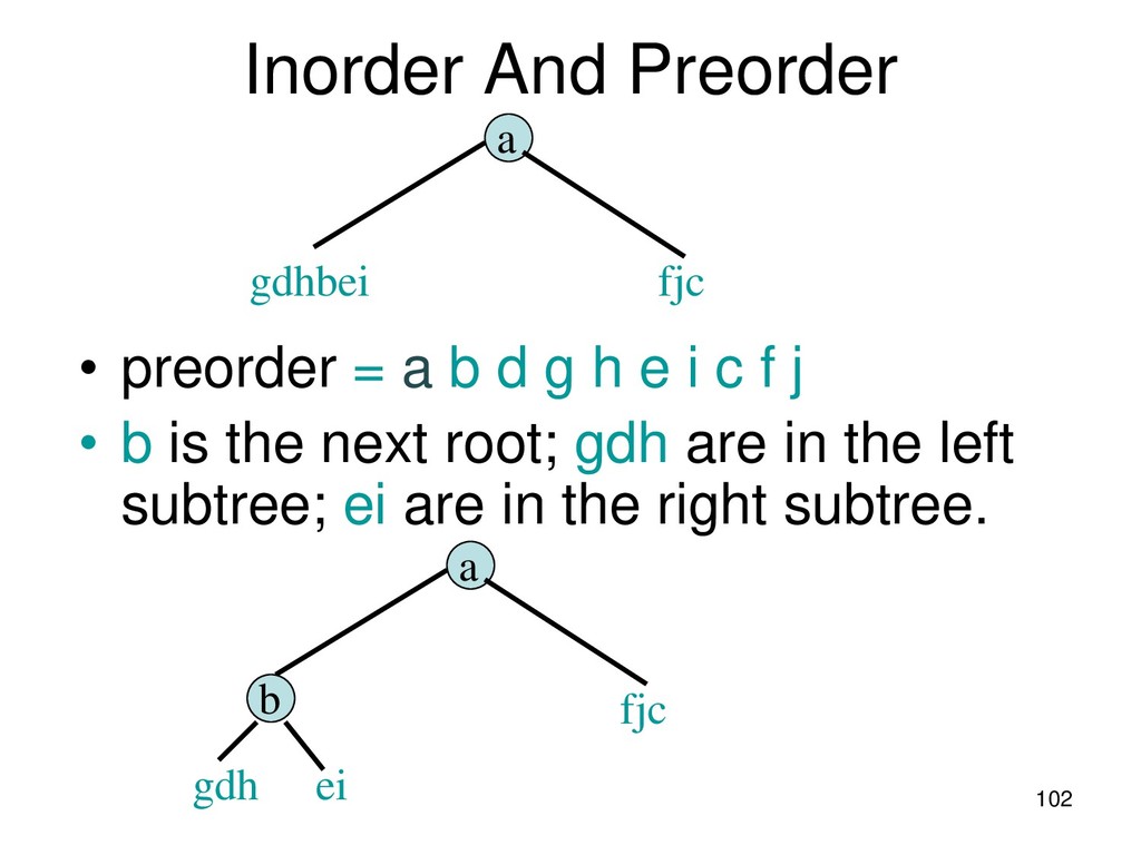
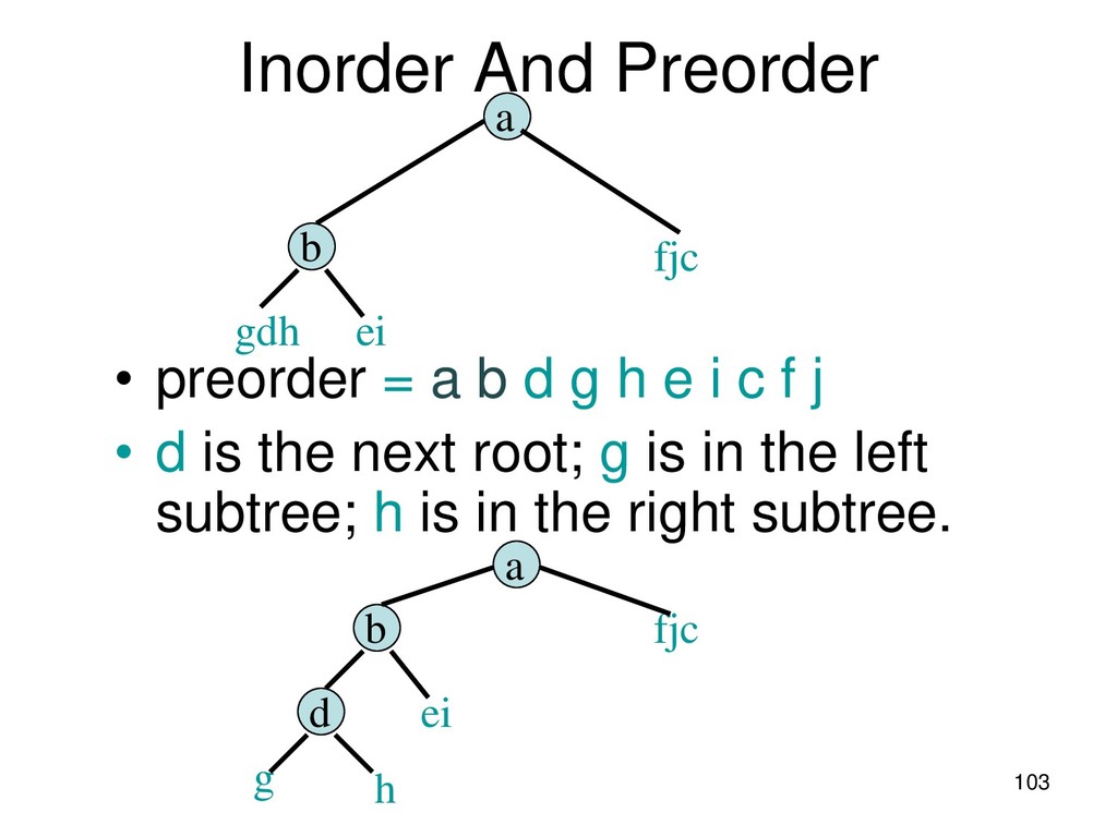
b e i a f j c • preorder = a b d g h e i c f j • Scan the preorder left to right using the inorder to separate left and right subtrees. • a is the root of the tree; gdhbei are in the left subtree; fjc are in the right subtree. a gdhbei fjc
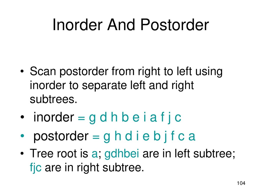
left using inorder to separate left and right subtrees. • inorder = g d h b e i a f j c • postorder = g h d i e b j f c a • Tree root is a; gdhbei are in left subtree; fjc are in right subtree.
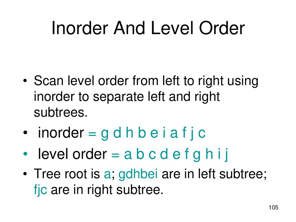
left to right using inorder to separate left and right subtrees. • inorder = g d h b e i a f j c • level order = a b c d e f g h i j • Tree root is a; gdhbei are in left subtree; fjc are in right subtree.
– Max Priority Queue • What can Priority Queue do? – Sorting – Machine Schedule • Heap Tree • Leftist Tree – Extended binary tree • Binary Search Tree • Selection Tree 106
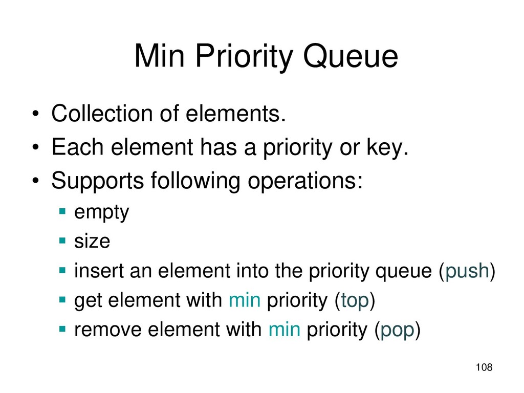
element has a priority or key. • Supports following operations: ▪ empty ▪ size ▪ insert an element into the priority queue (push) ▪ get element with min priority (top) ▪ remove element with min priority (pop)
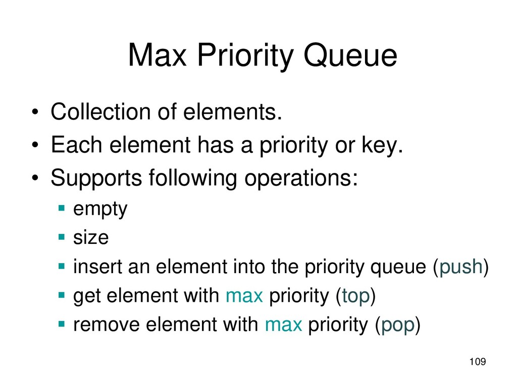
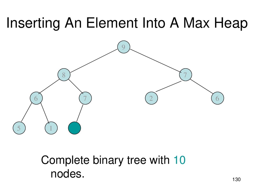
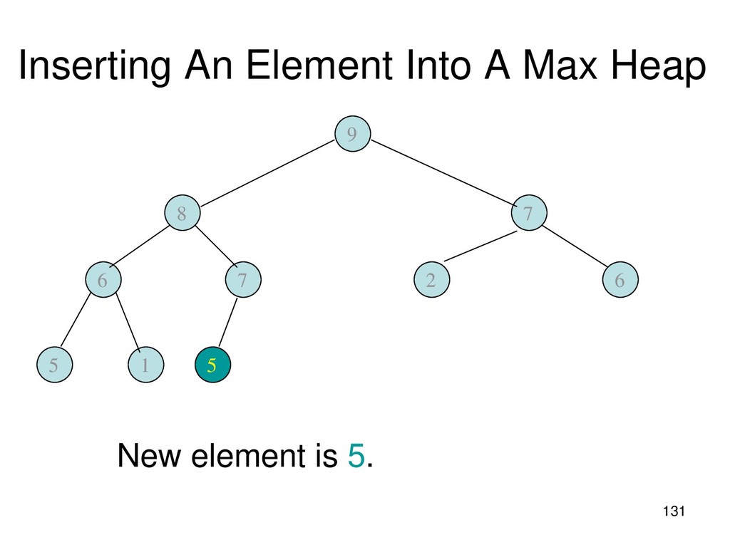
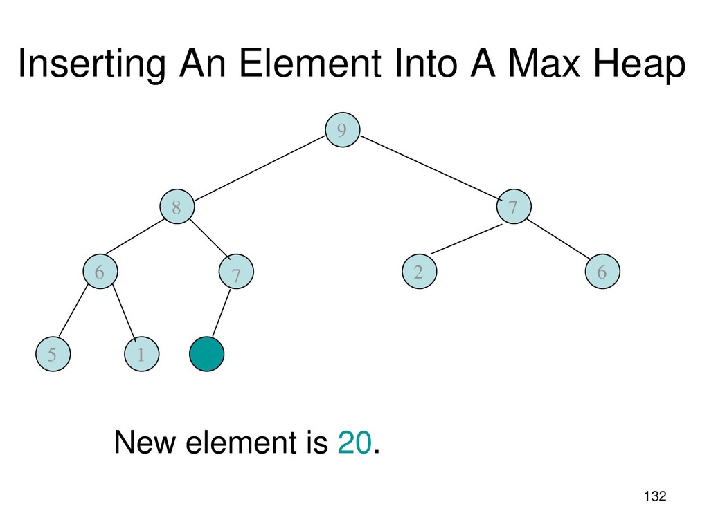
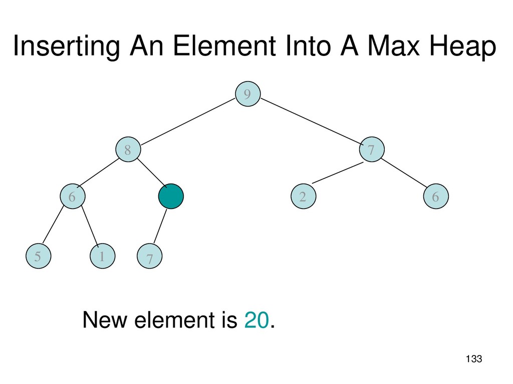
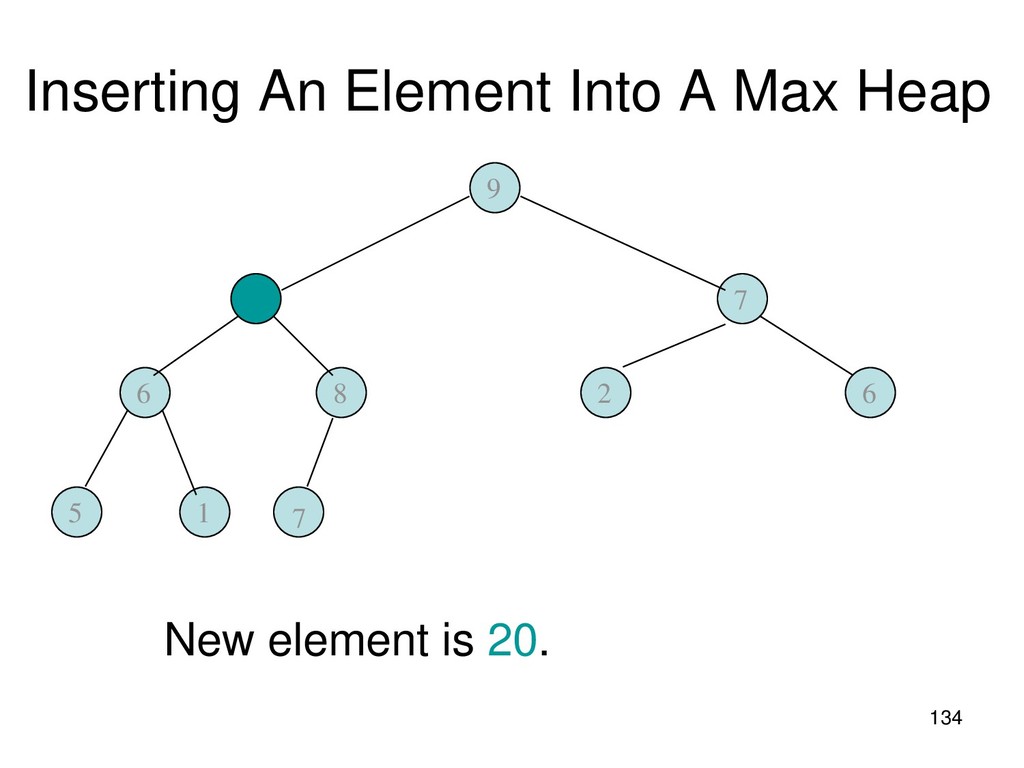
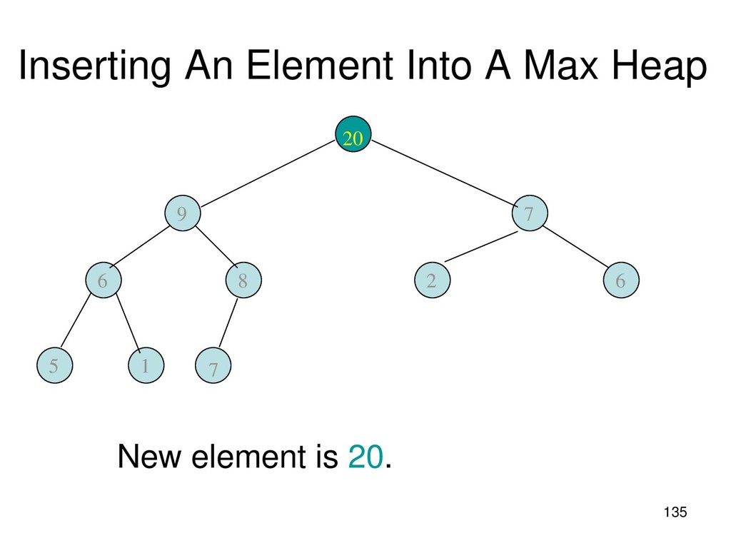
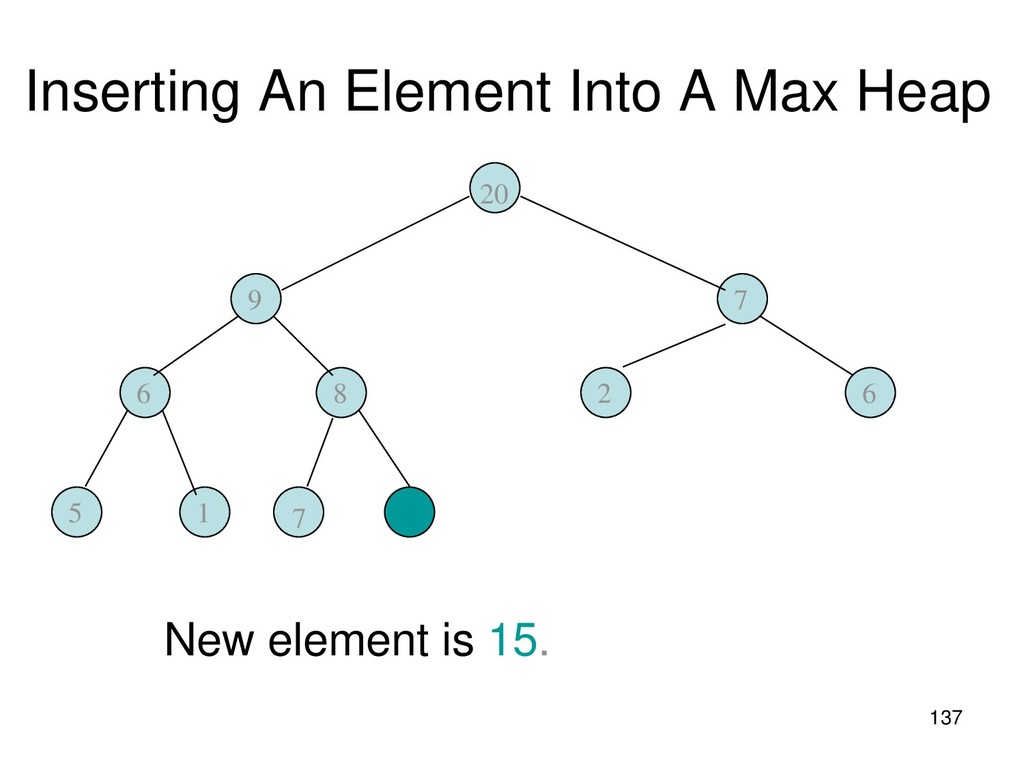
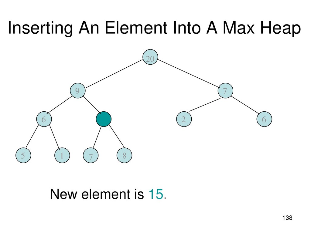
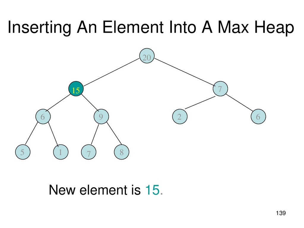
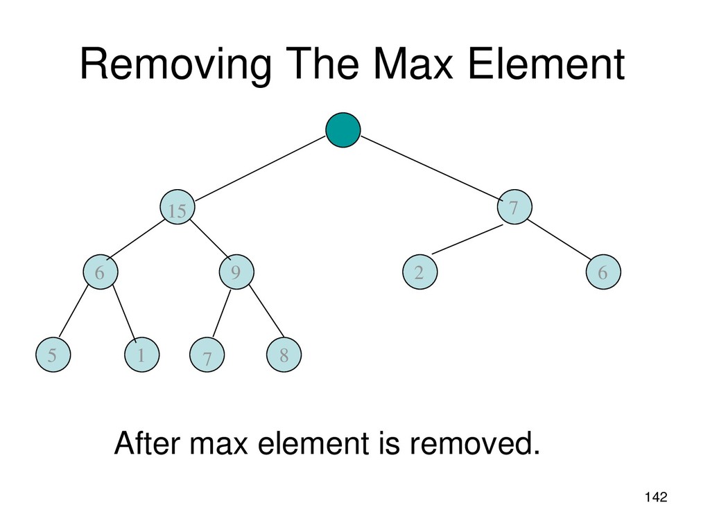
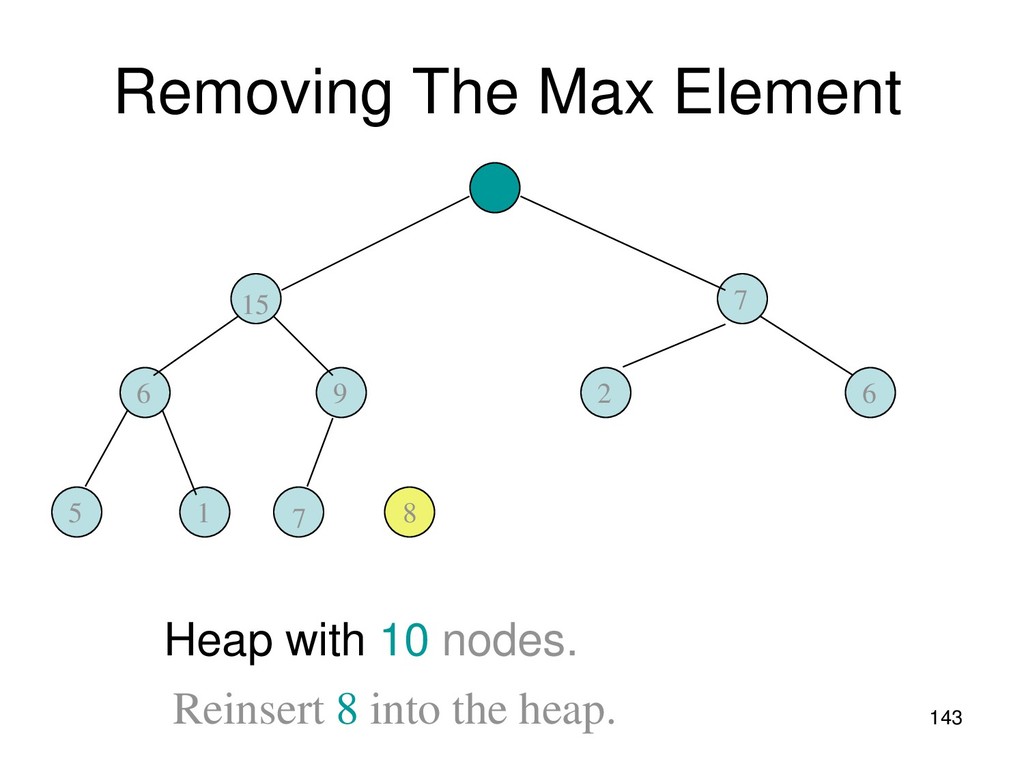
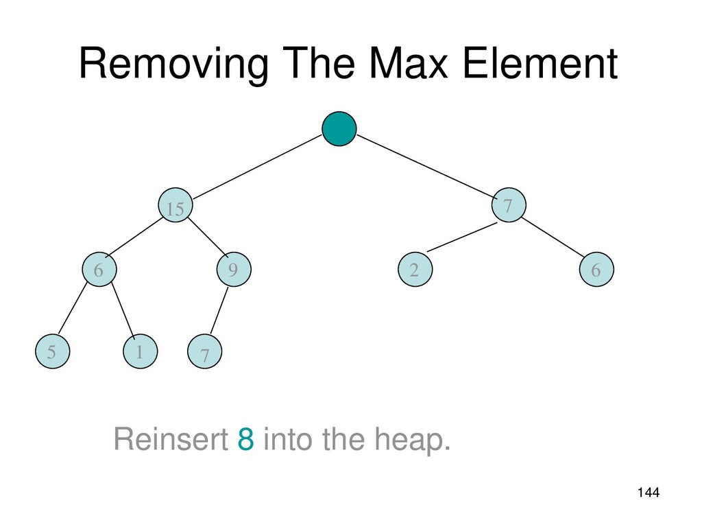
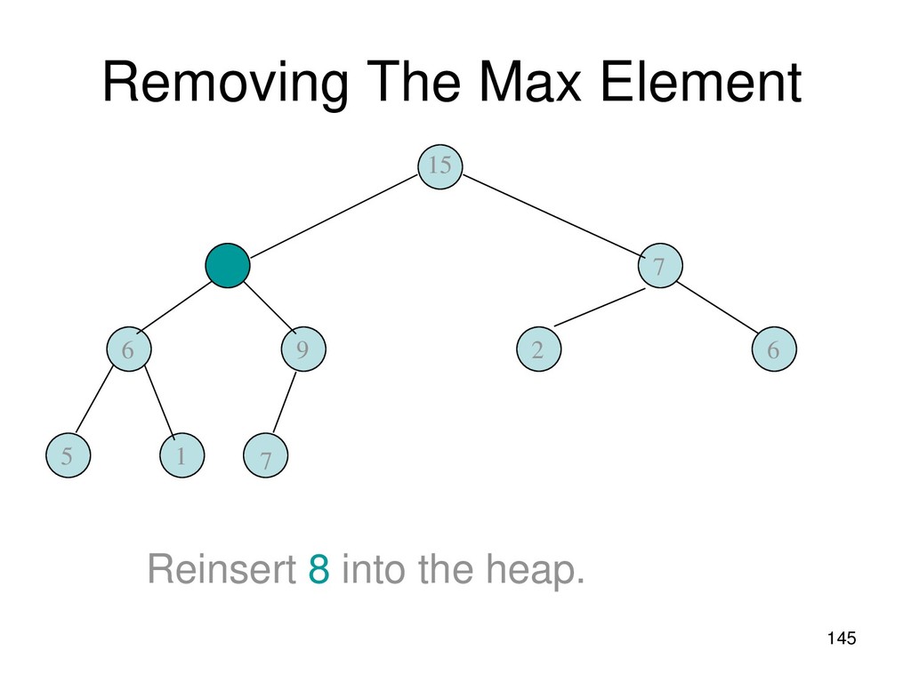
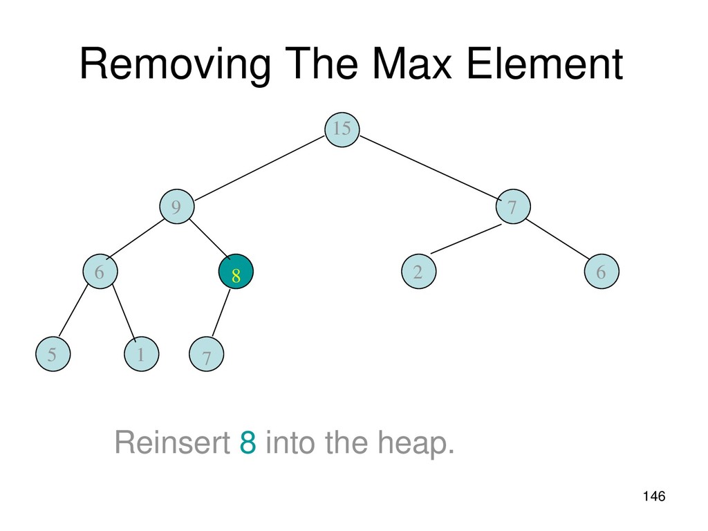
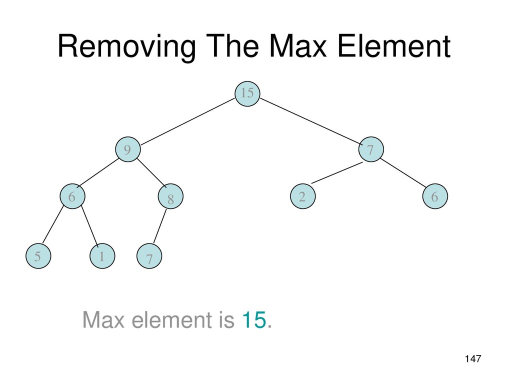
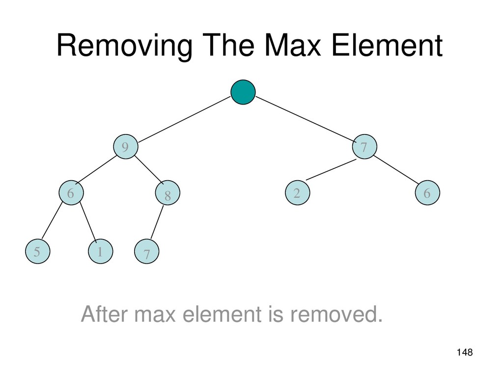
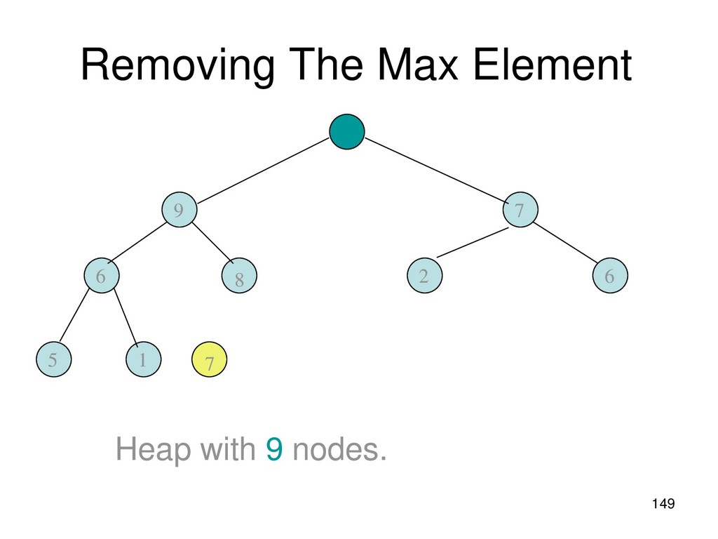
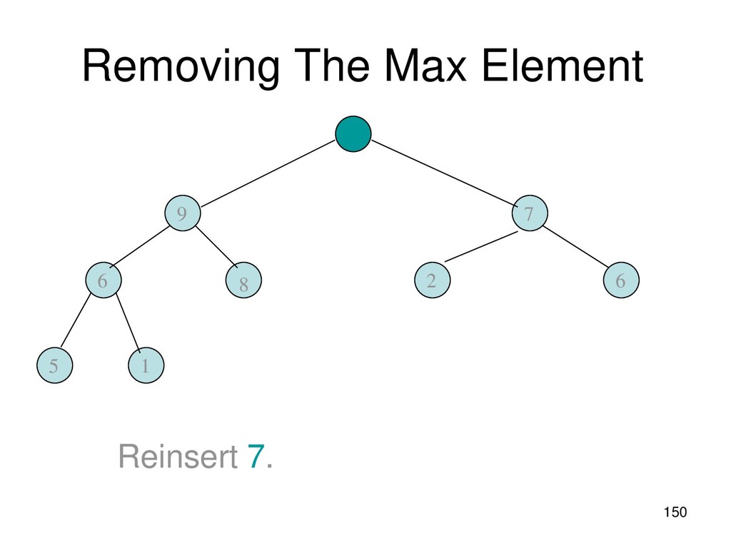
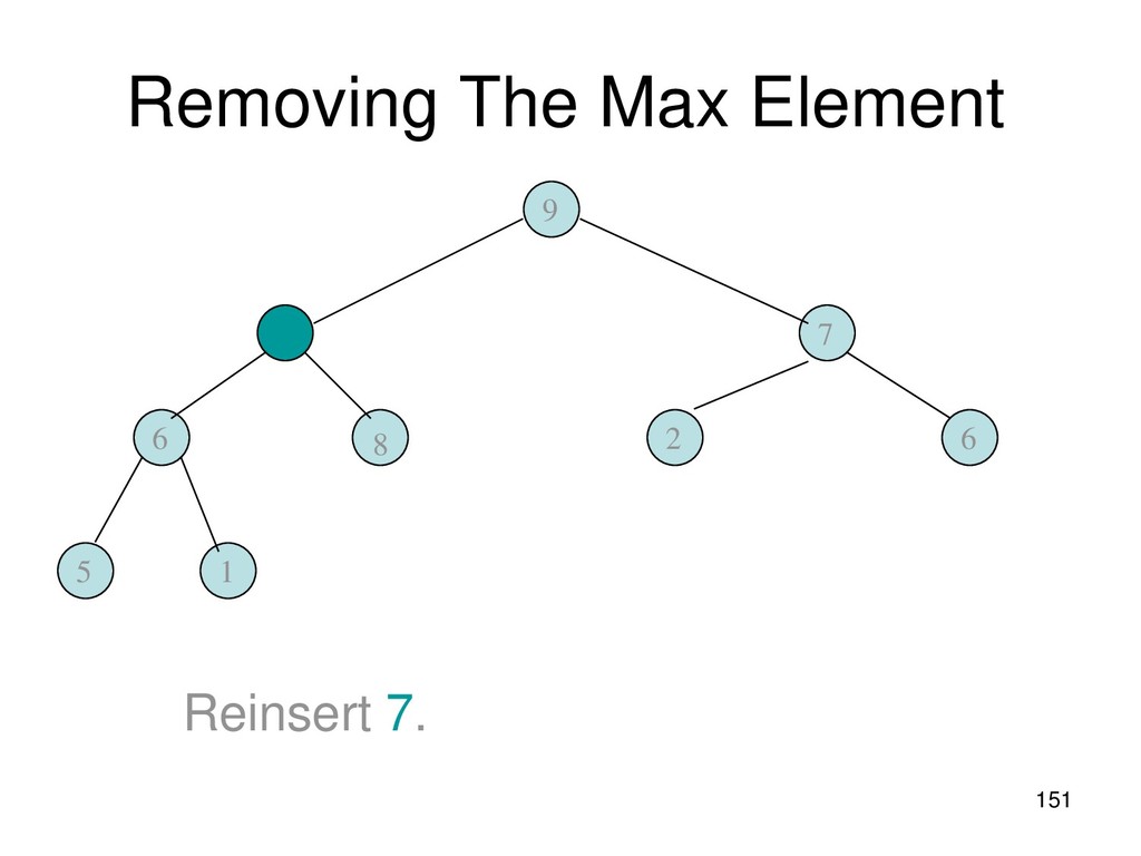
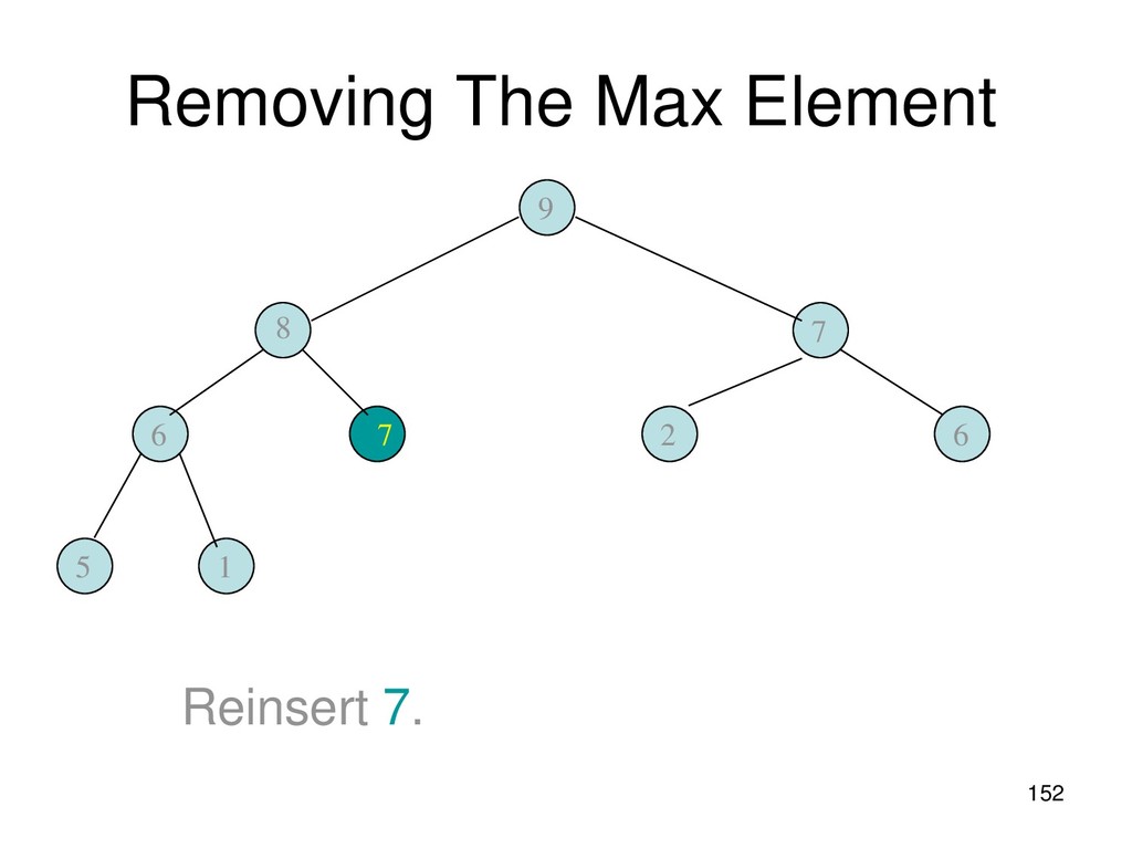
element has a priority or key. • Supports following operations: ▪ empty ▪ size ▪ insert an element into the priority queue (push) ▪ get element with max priority (top) ▪ remove element with max priority (pop)
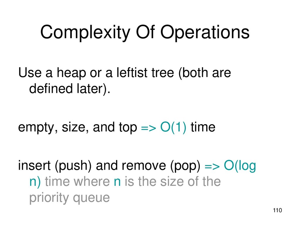
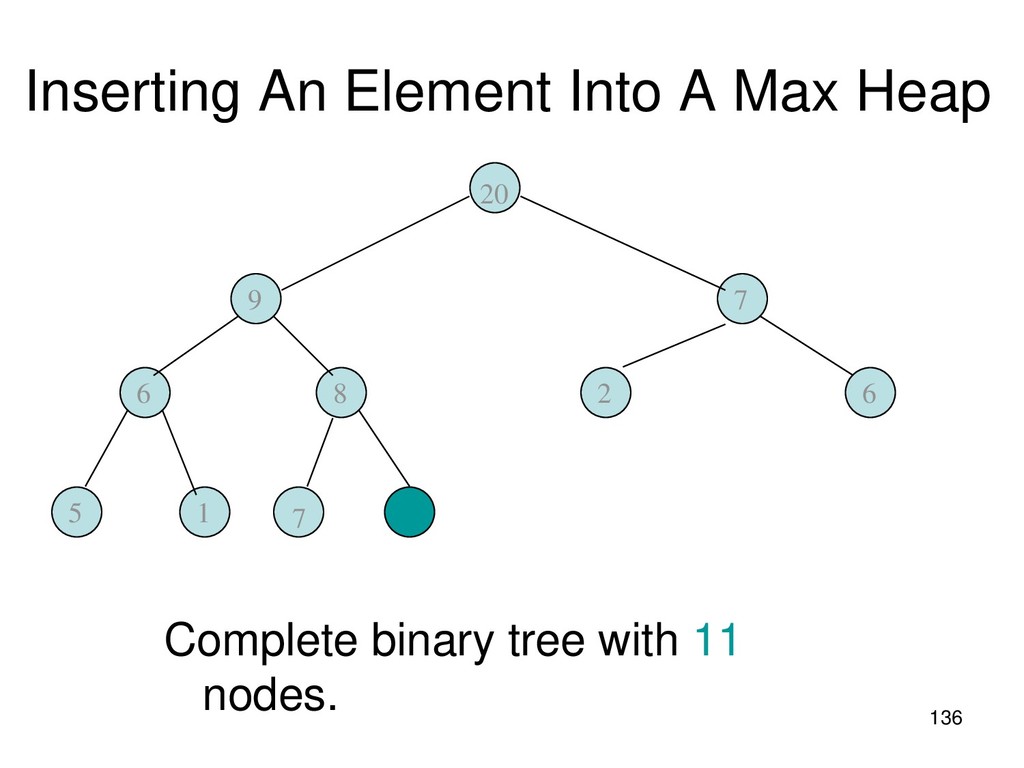
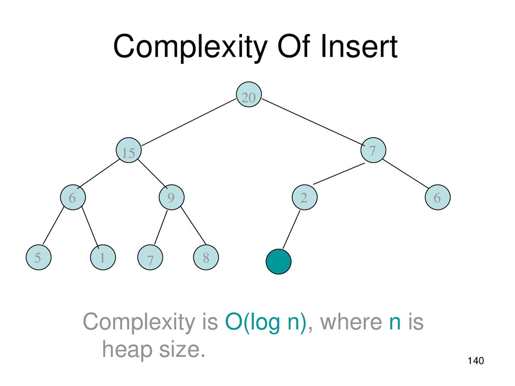
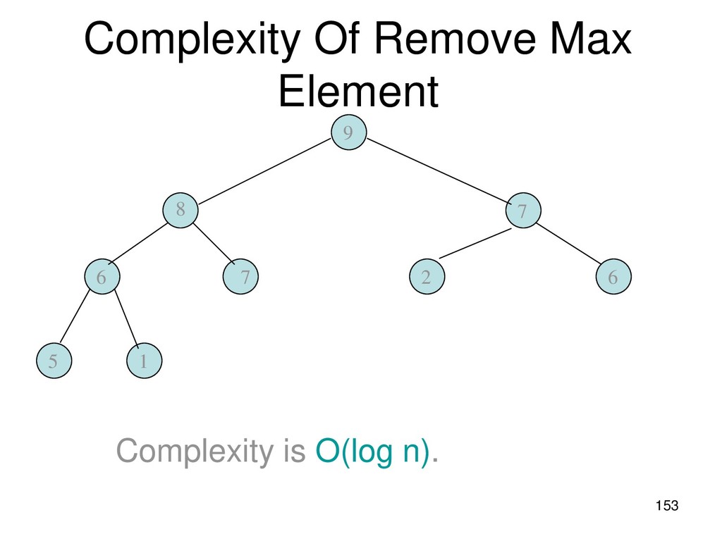
tree (both are defined later). empty, size, and top => O(1) time insert (push) and remove (pop) => O(log n) time where n is the size of the priority queue
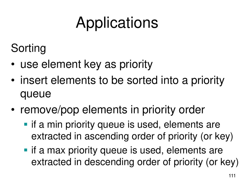
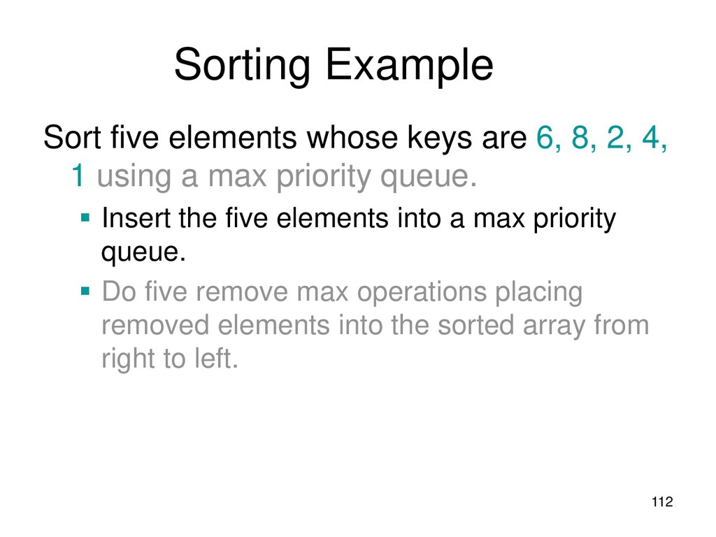
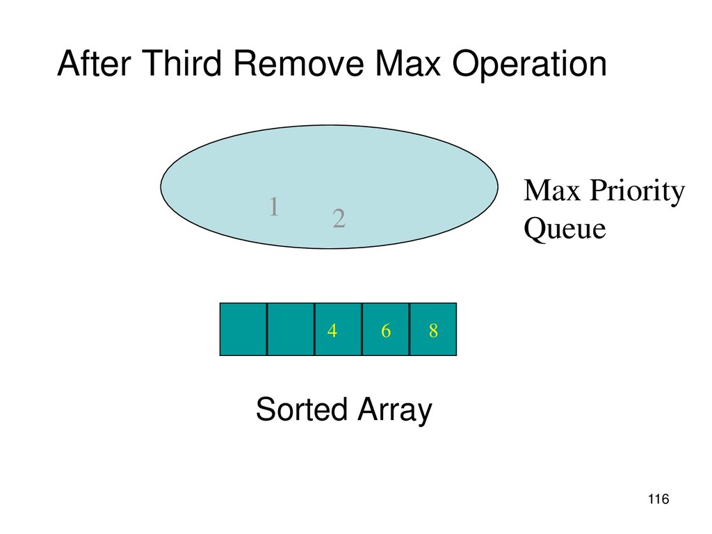
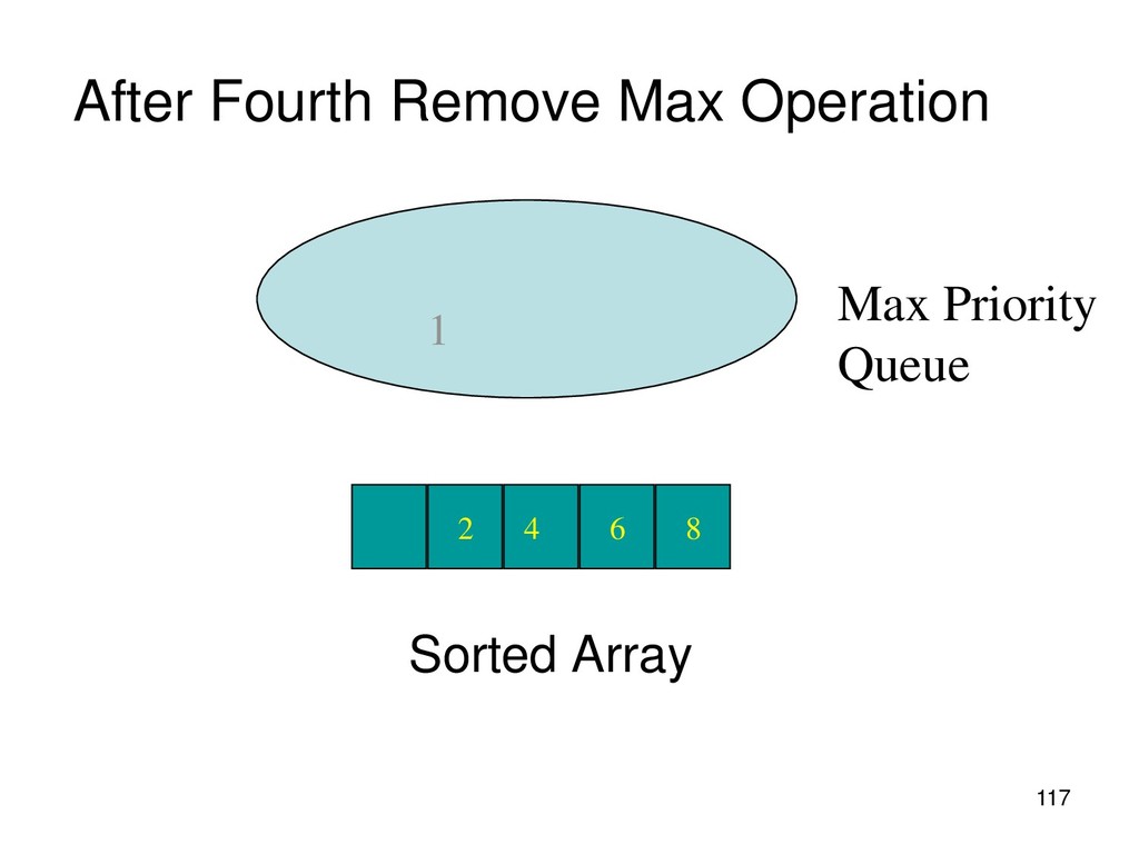
insert elements to be sorted into a priority queue • remove/pop elements in priority order ▪ if a min priority queue is used, elements are extracted in ascending order of priority (or key) ▪ if a max priority queue is used, elements are extracted in descending order of priority (or key)
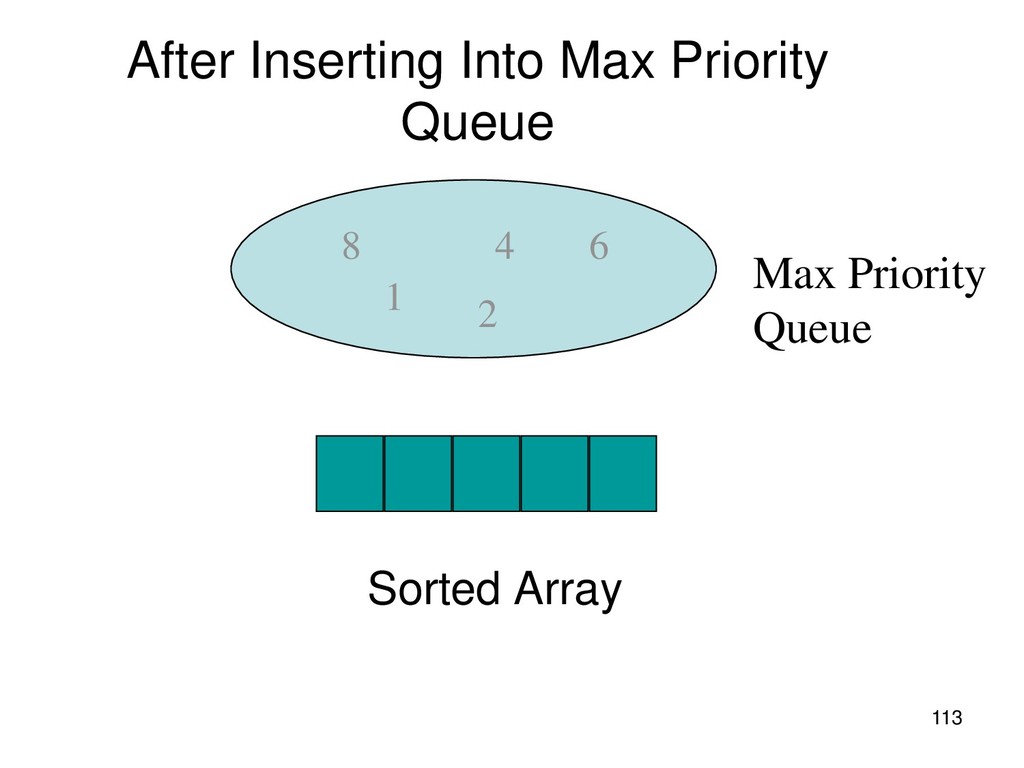
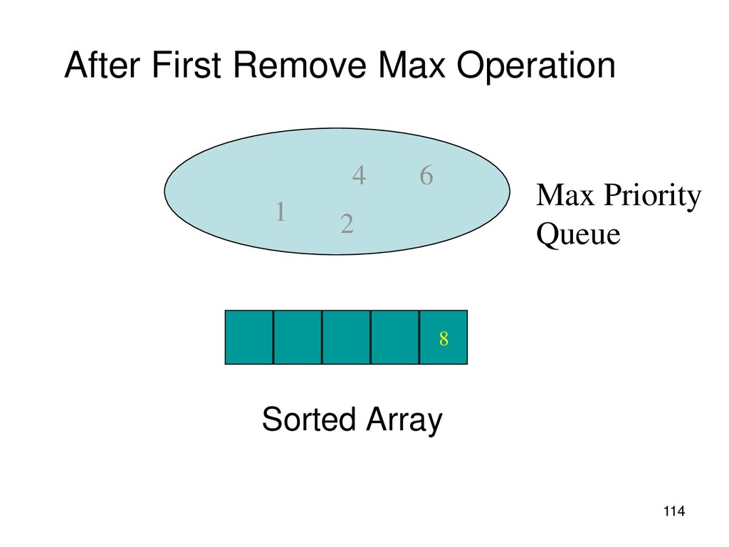
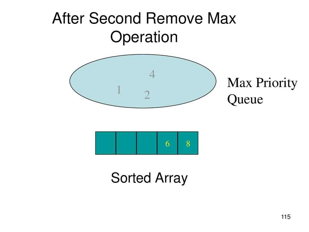
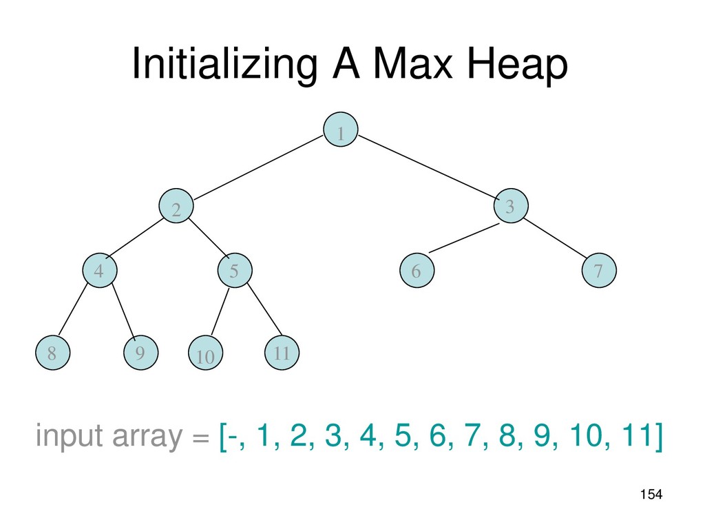
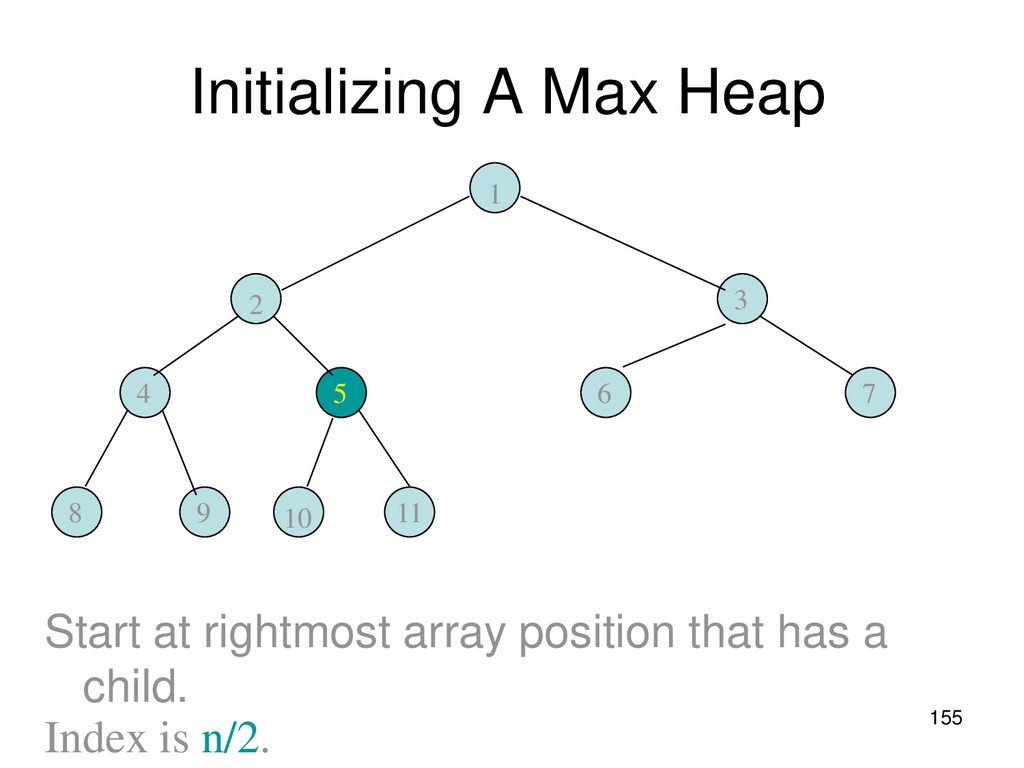
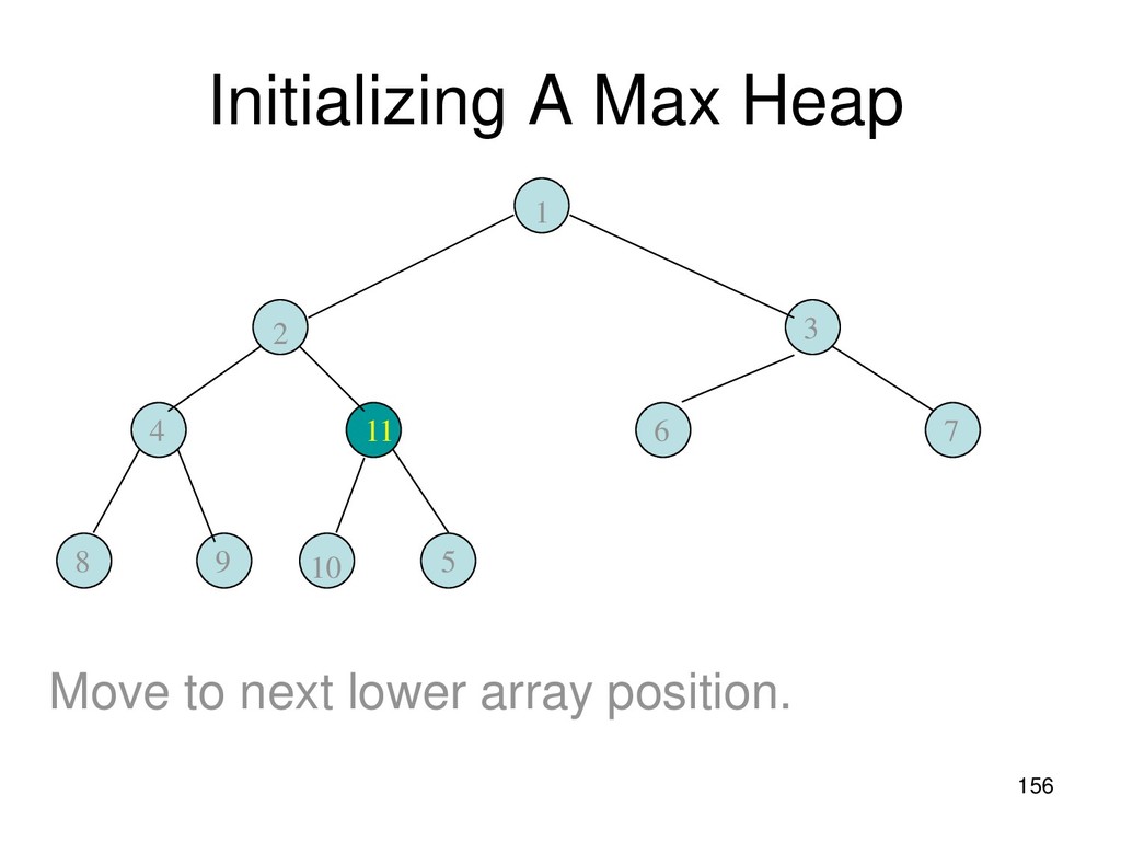
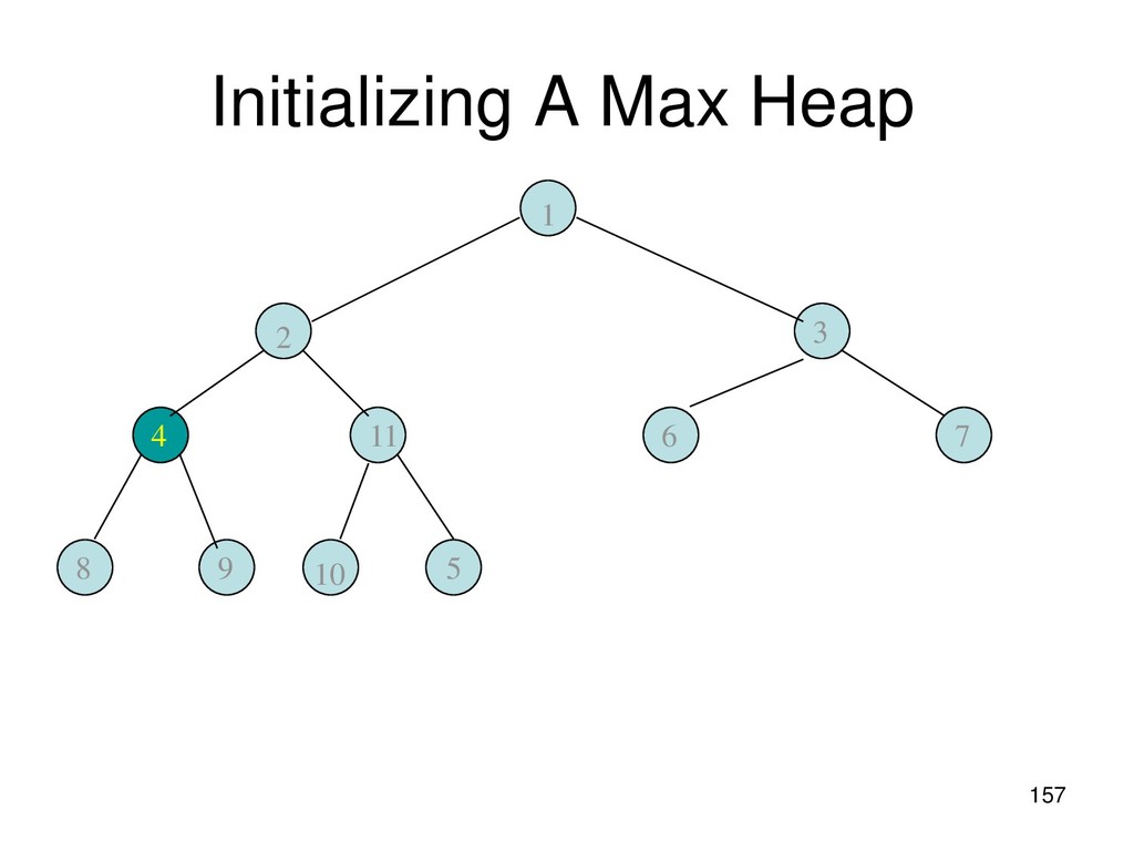
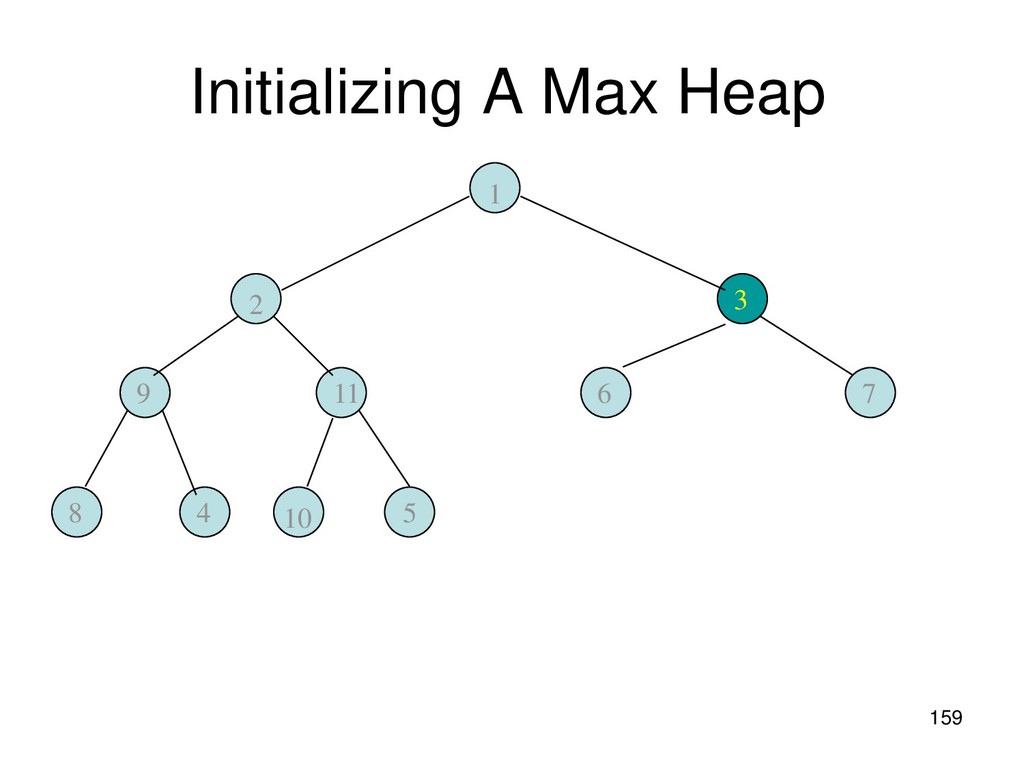
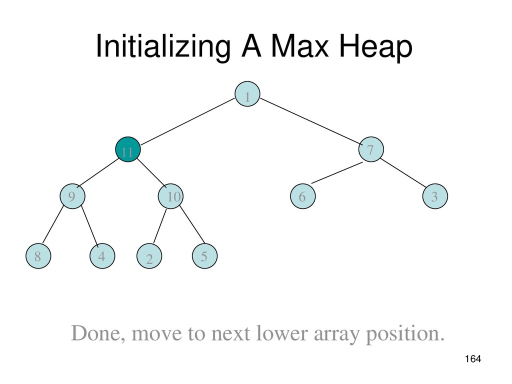
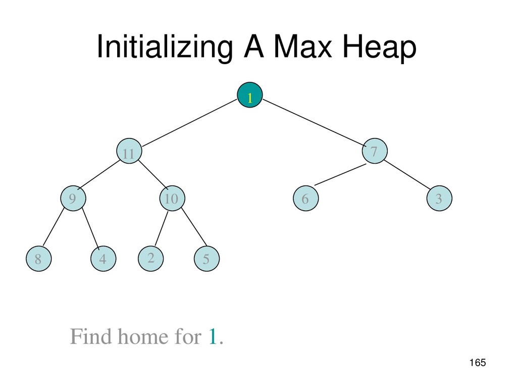
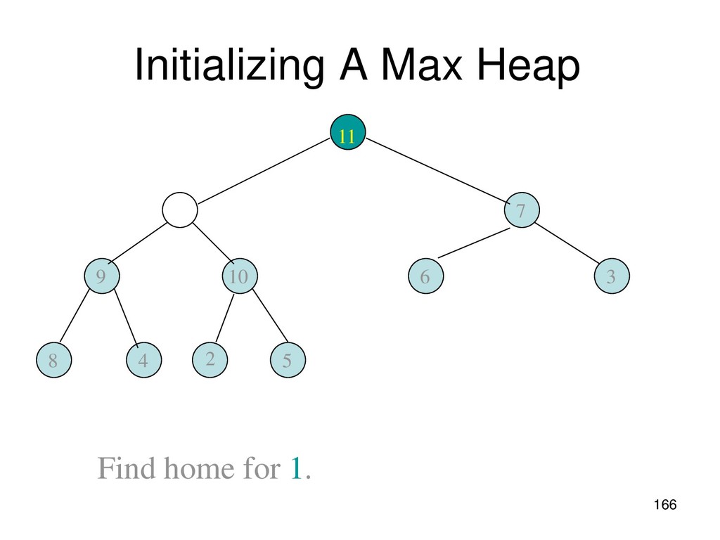
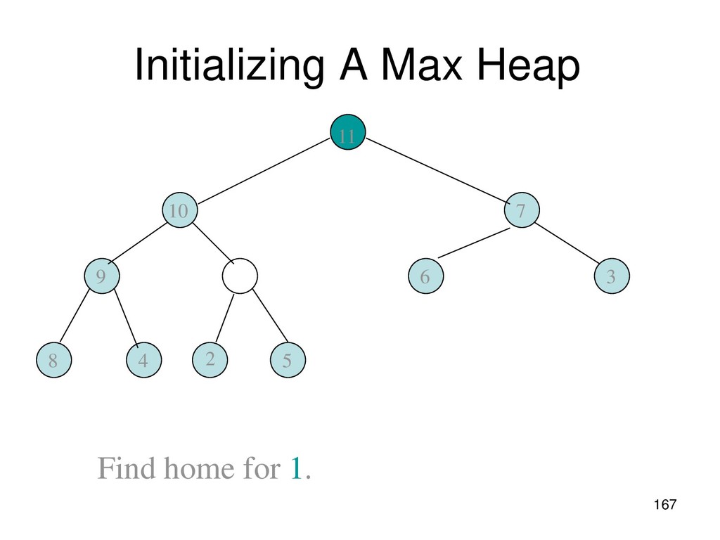
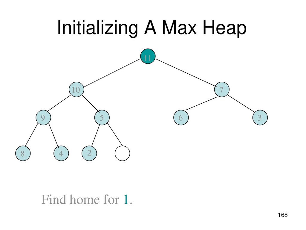
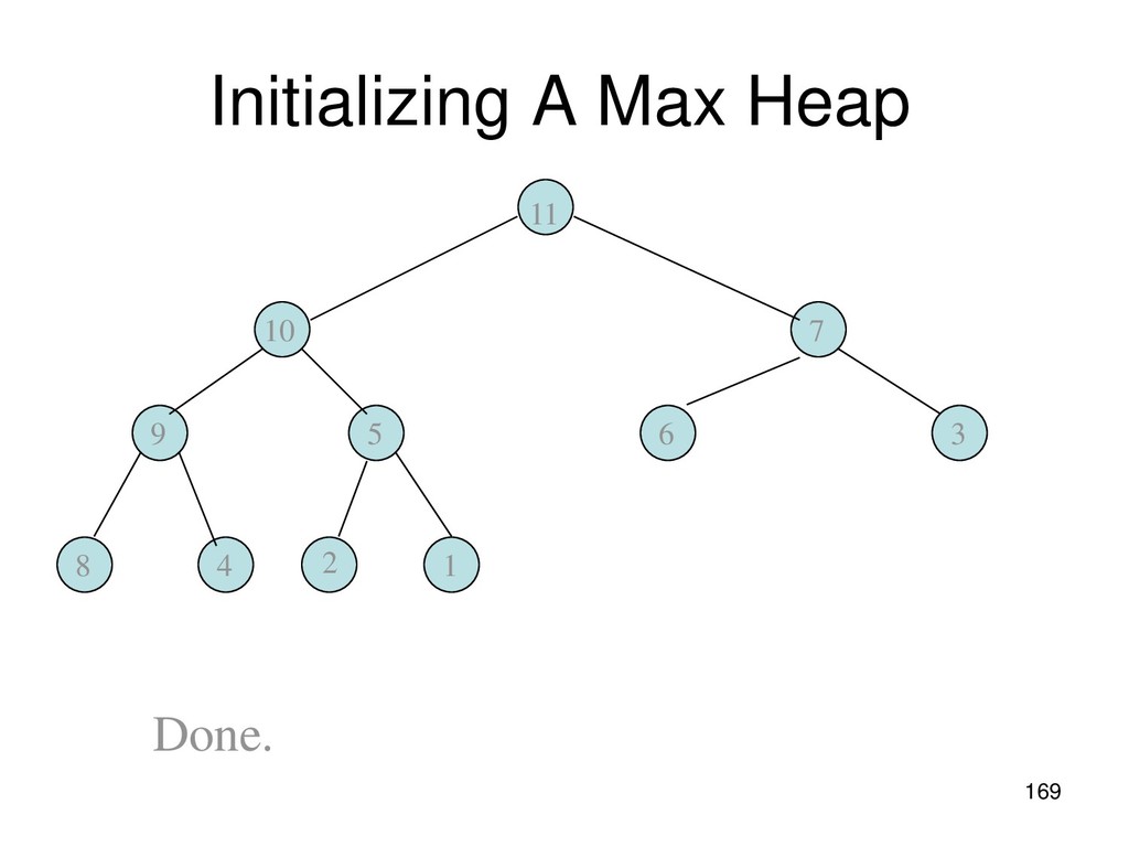
8, 2, 4, 1 using a max priority queue. ▪ Insert the five elements into a max priority queue. ▪ Do five remove max operations placing removed elements into the sorted array from right to left.