"Embedding words in low-dimensional spaces" by Piotr Mirowski, Research Scientist at Google

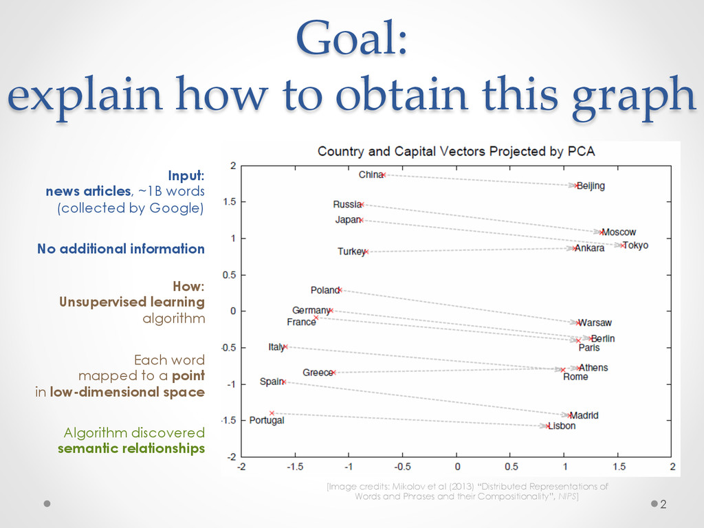
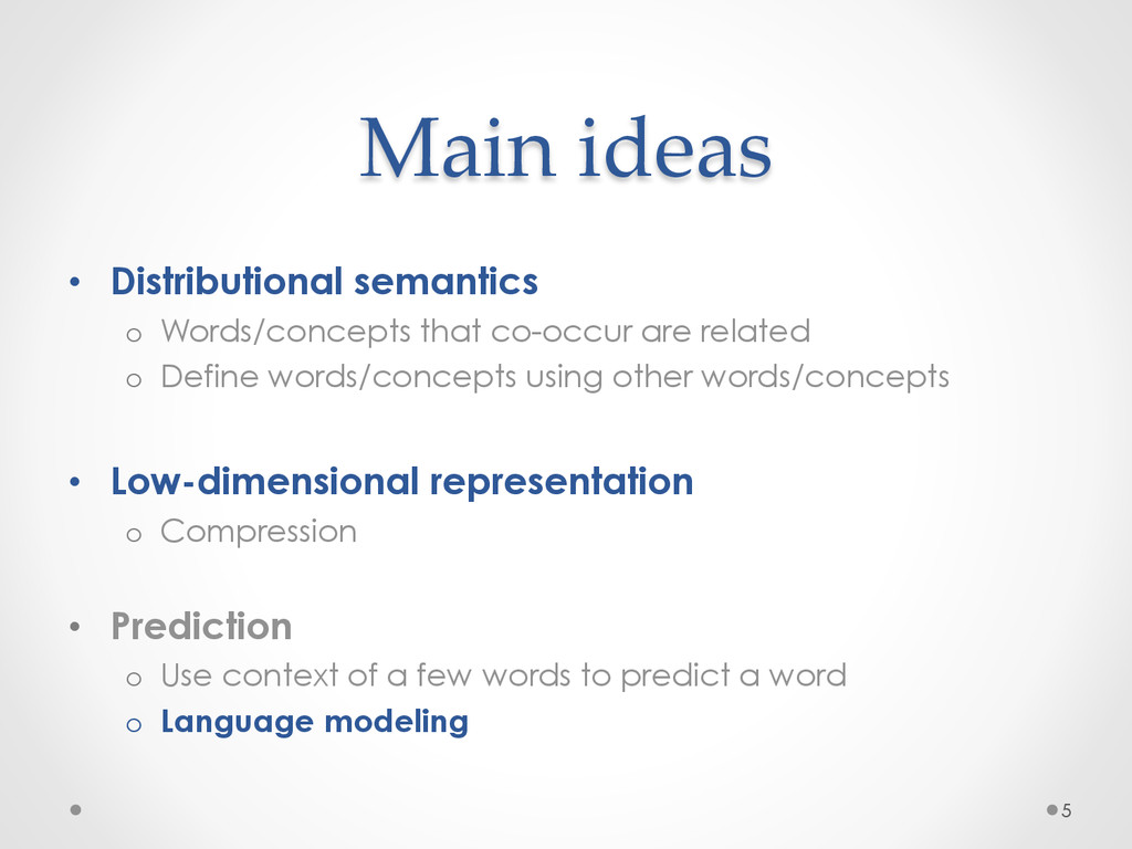
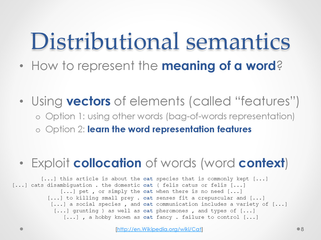
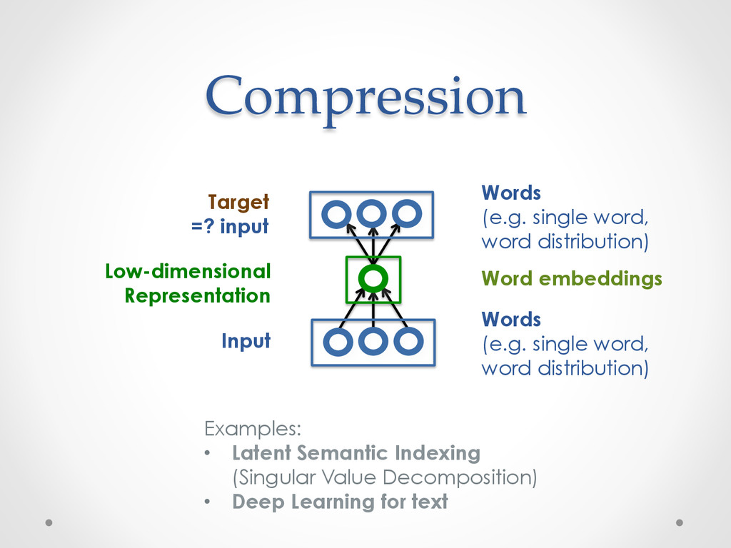
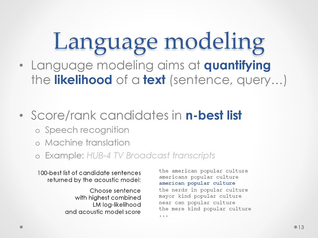
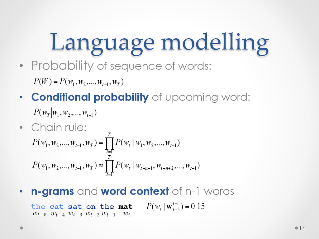
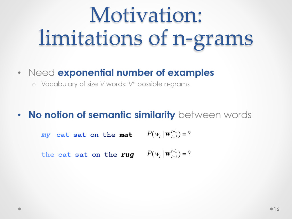
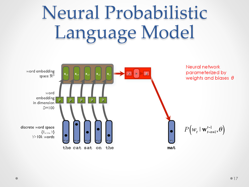
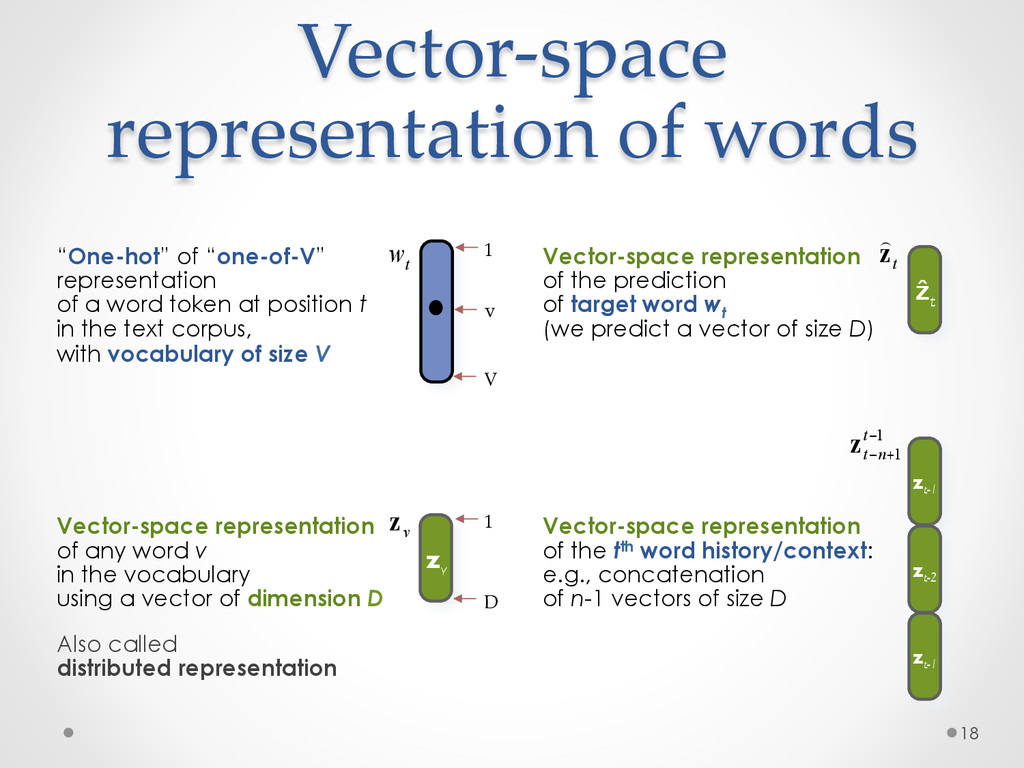
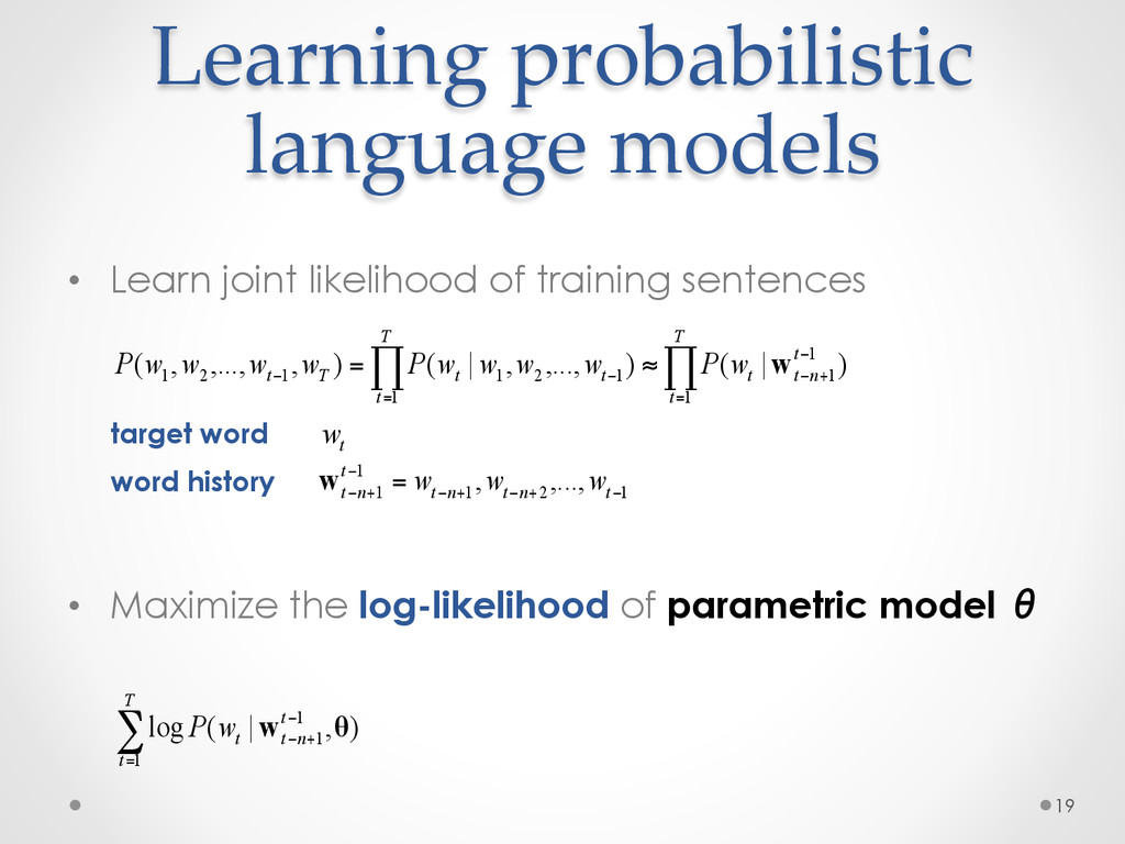
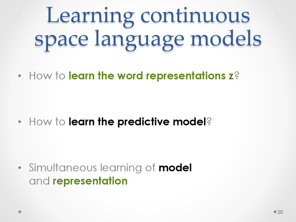
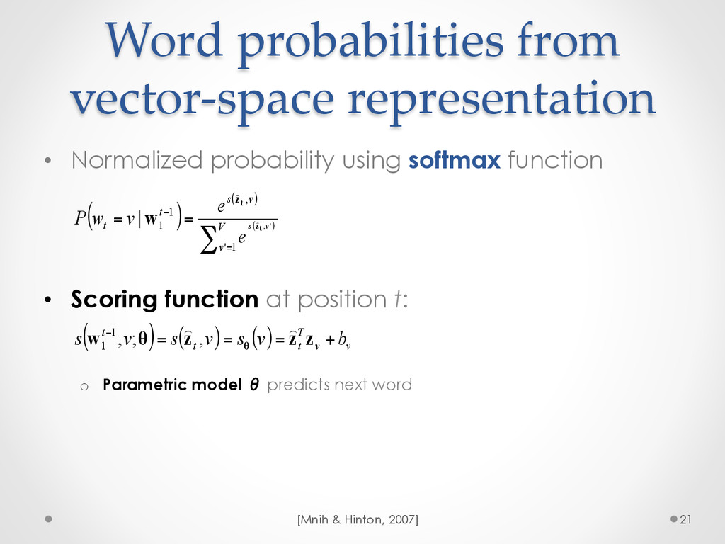
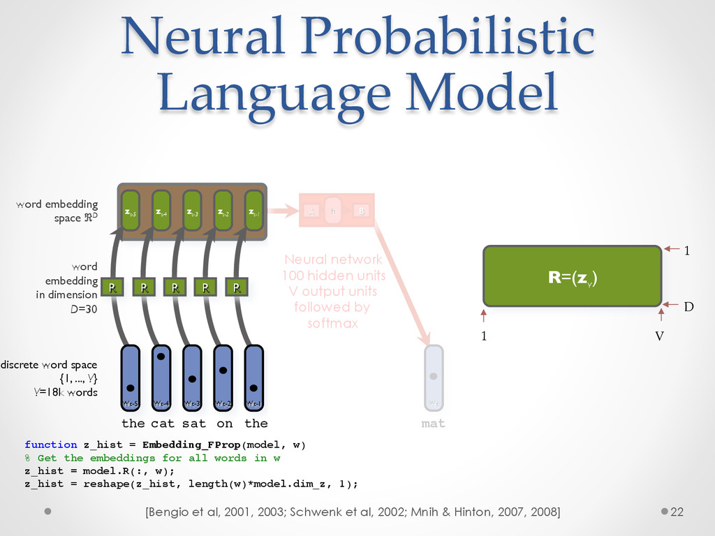
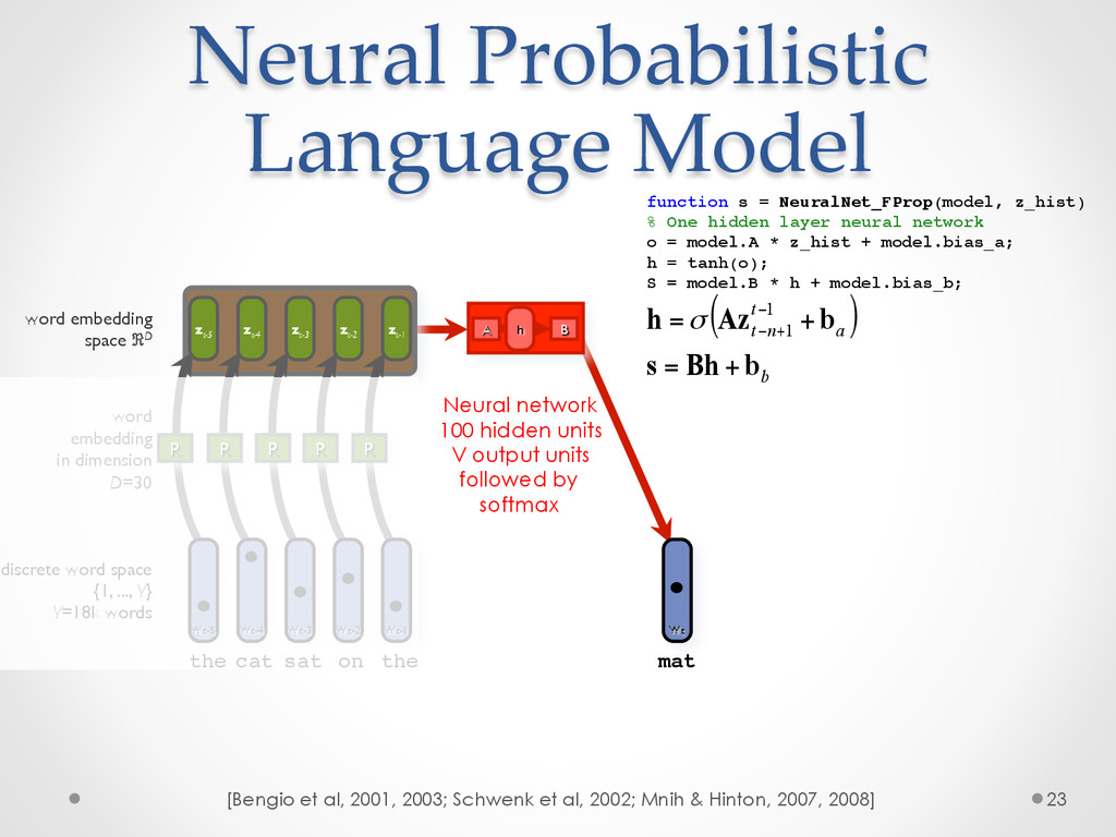
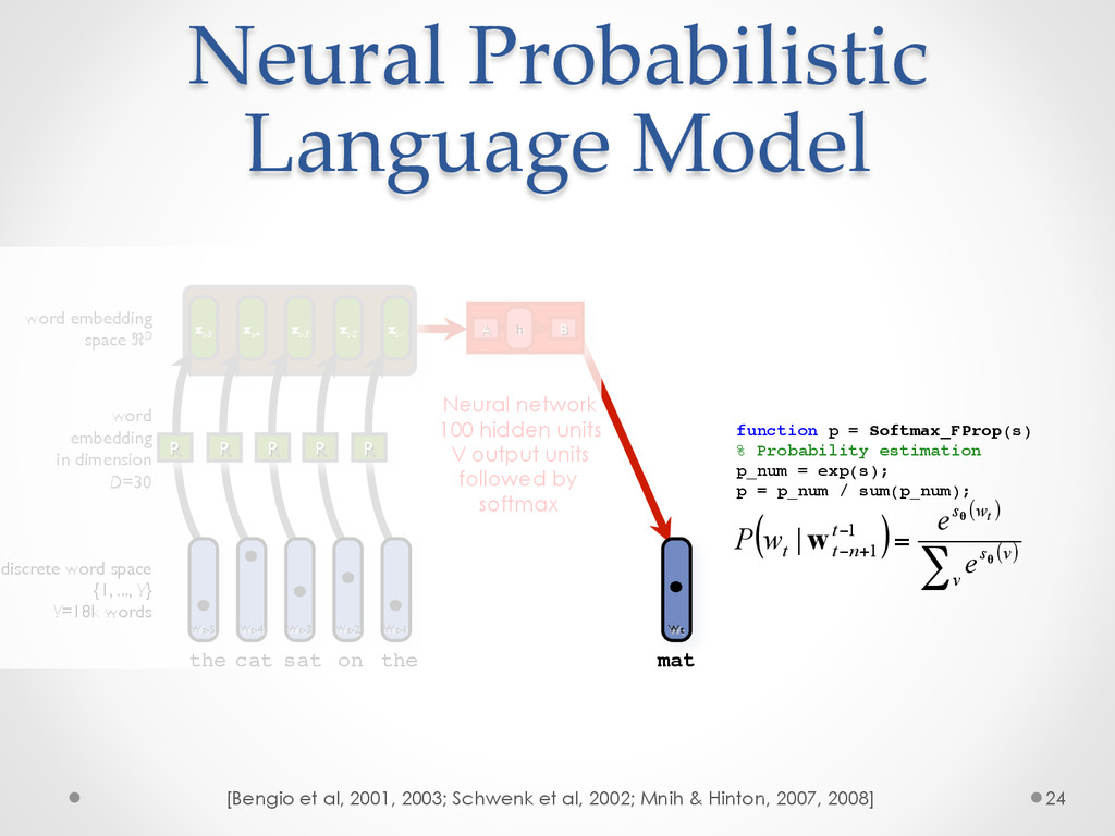
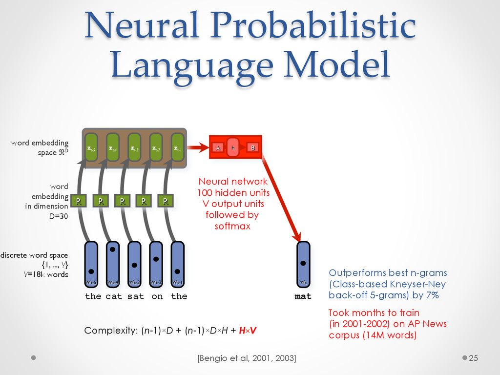
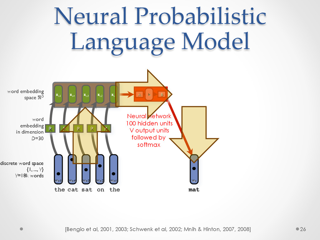
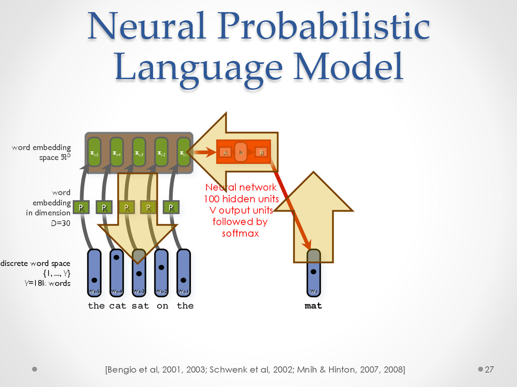
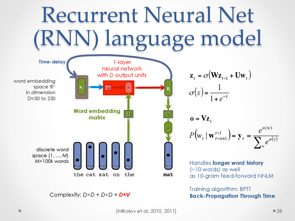
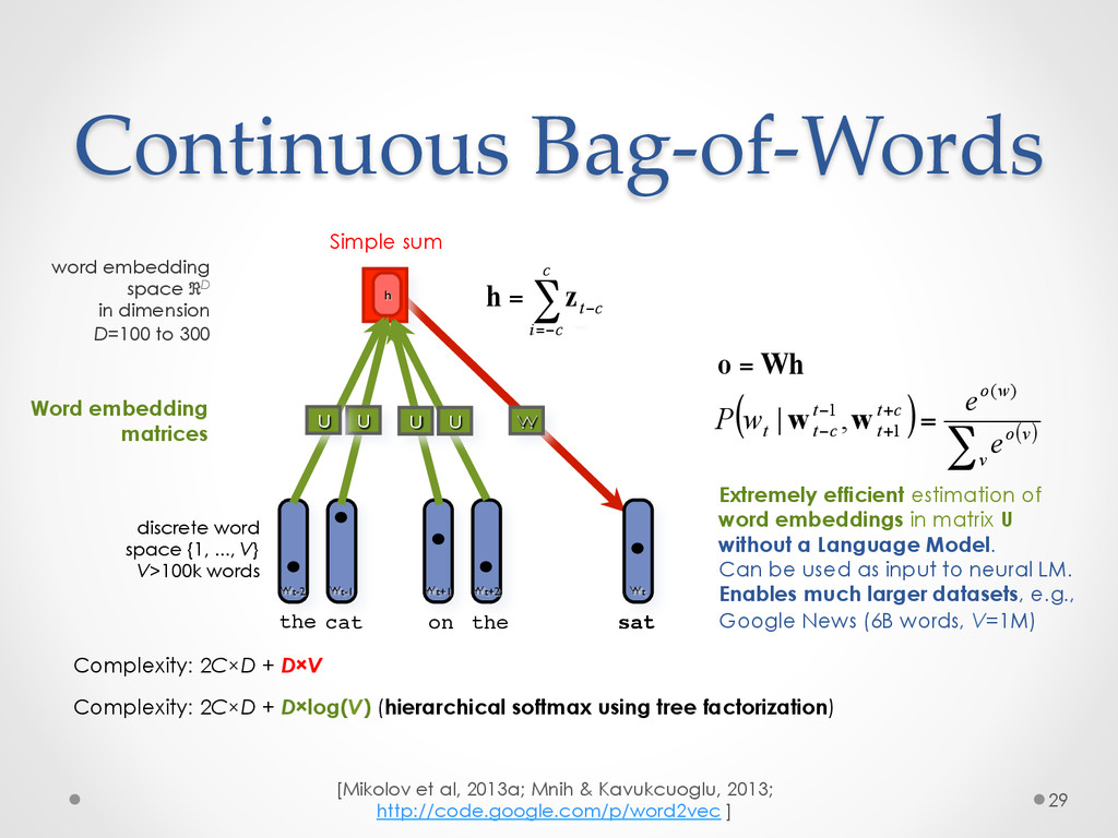
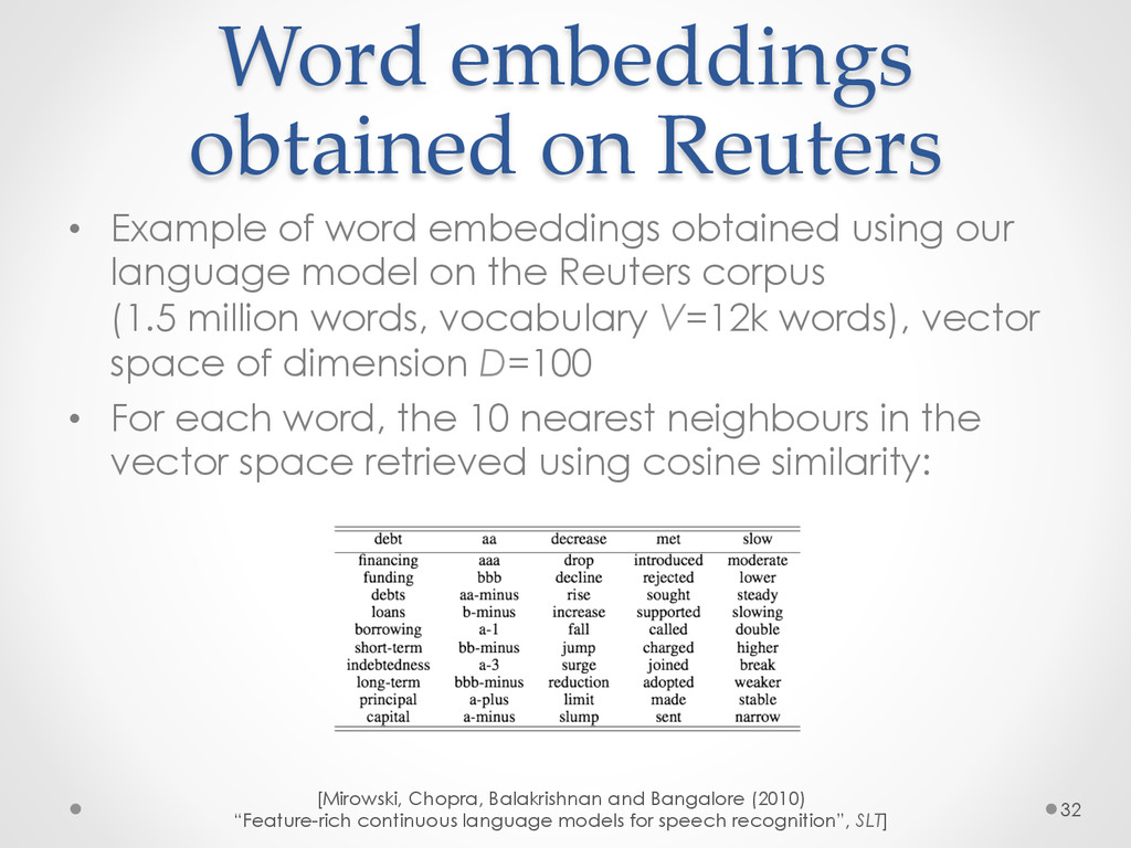
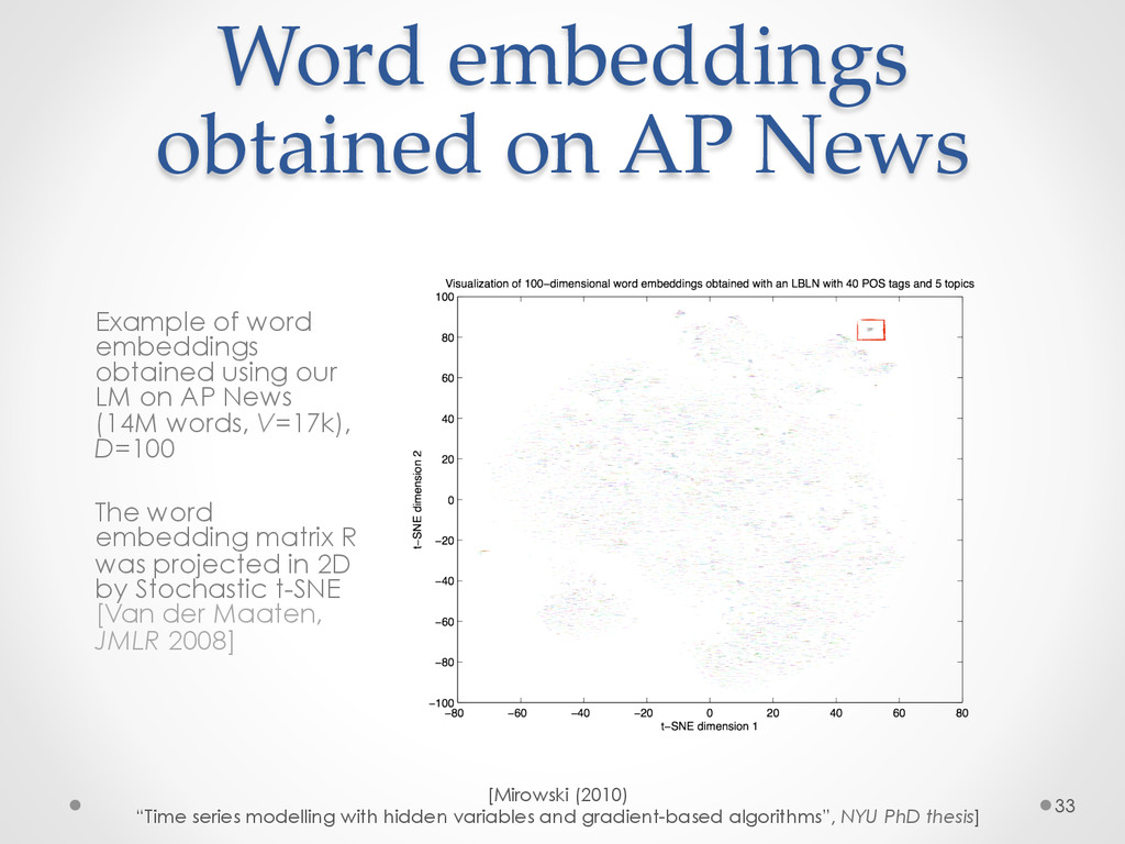
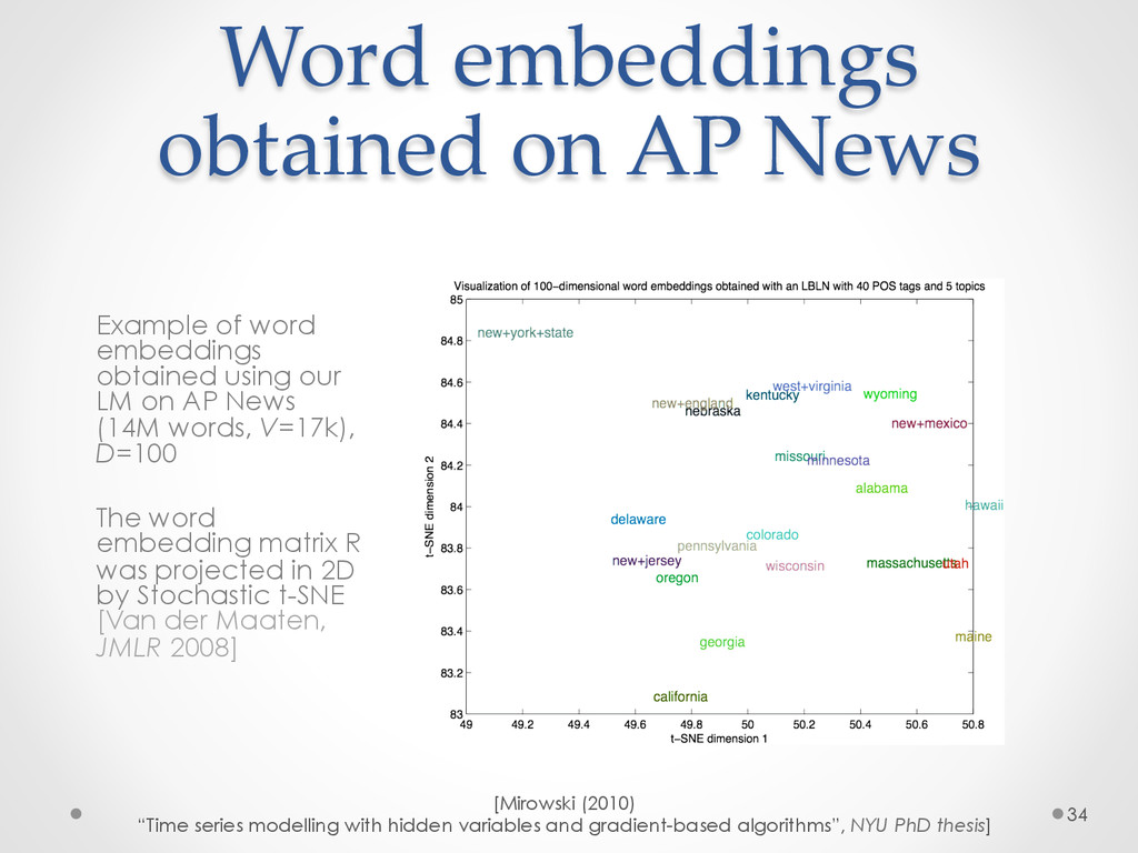
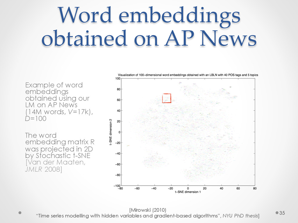
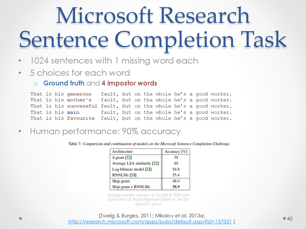
A recent development in statistical language modelling happened when distributional semantics (the idea of defining words in relation to other words) met neural networks. Neural language models further try to "embed" each word into a low-dimensional vector-space representation that can be learned as the language model is trained. When they are trained on very large corpora, these models can not only achieve state-of-the-art performance in many applications such as speech recognition, but also help visualising graphs of word relationships or even two-dimensional maps of word meanings.

Transcript

1. Embedding  words   in  low-­‐‑dimensional   spaces Piotr Mirowski Advanced Data Visualization London Meetup November 6, 2014
2. Goal:   explain  how  to  obtain  this  graph 2 Input: news articles, ~1B words (collected by Google) [Image credits: Mikolov et al (2013) “Distributed Representations of Words and Phrases and their Compositionality”, NIPS] How: Unsupervised learning algorithm No additional information Each word mapped to a point in low-dimensional space Algorithm discovered semantic relationships
3. Outline •  Main ideas o  Distributional semantics o  Compression (low-dimensional representation) o  Probabilistic language models (LMs) and n-grams •  Neural Probabilistic LMs o  Vector-space representation of words o  Neural probabilistic language model o  Recurrent Neural Network LMs o  Continuous bag-of-words and skip-gram models •  Applications o  Word representation o  Sentence completion and linguistic regularities 3
4. Outline •  Main ideas o  Distributional semantics o  Compression (low-dimensional representation) o  Probabilistic language models (LMs) and n-grams •  Neural Probabilistic LMs o  Vector-space representation of words o  Neural probabilistic language model o  Recurrent Neural Network LMs o  Continuous bag-of-words and skip-gram models •  Applications o  Word representation o  Sentence completion and linguistic regularities 4
5. Main  ideas •  Distributional semantics o  Words/concepts that co-occur are related o  Define words/concepts using other words/concepts •  Low-dimensional representation o  Compression •  Prediction o  Use context of a few words to predict a word o  Language modeling 5
6. Distributional  semantics (idea #1)
7. Word  representation •  Bag-of-words: words are tokens in vocabulary of size V •  Distributions of words 7 0 200000 400000 600000 800000 1000000 1200000 <proper_noun> </s> , the . <unknown> of to and a #n in `` 'ʹ'ʹ 'ʹs said for he was is -­‐‑ on with by his ) ( but have at as an who are were i ; not has be had #an will #$n : about would or people after Token  count  (top  50)  –  Corpus:  AP  News  (1995),  16M  words,  V=17965 0 5 10 15 20 25 30 35 dig_out tung tempted diagnose crouch back_out looking_out envoys keepers chronicled pristine good_luck peabody john_lennon forgo co-­‐‑stars accommodation rush-­‐‑hour transitional harvests best_selling rooftops jaguar nameplate discrepancies lousy shotguns grammar staff_member calderon patriots proportional renomination lutheran walnut communications_equ logos pulls fielding beaumont collie weekday georges spat torrential handmade tax_deduction appropriations_bill jubilant ticket-­‐‑holders Token  count  (boeom  50)  –  Corpus:  AP  News  (1995)
8.   Distributional  semantics •  How to represent the meaning of a word? •  Using vectors of elements (called “features”) o  Option 1: using other words (bag-of-words representation) o  Option 2: learn the word representation features •  Exploit collocation of words (word context) 8 [...] this article is about the cat species that is commonly kept [...] [...] cats disambiguation . the domestic cat ( felis catus or felis [...] [...] pet , or simply the cat when there is no need [...] [...] to killing small prey . cat senses fit a crepuscular and [...] [...] a social species , and cat communication includes a variety of [...] [...] grunting ) as well as cat pheromones , and types of [...] [...] , a hobby known as cat fancy . failure to control [...] [http://en.Wikipedia.org/wiki/Cat]
9. Low-­‐‑dimensional   representation (idea #2)
10. Compression Low-dimensional Representation Input Target =? input Examples: •  Latent Semantic Indexing (Singular Value Decomposition) •  Deep Learning for text Words (e.g. single word, word distribution) Words (e.g. single word, word distribution) Word embeddings
11. Prediction  and   language  modeling (idea #3)
12. Predicting  next  word   using  language  models 12 I always order pizza with cheese and mushrooms 0.15 pepperoni 0.1 anchovies 0.01 … fried rice 0.0001 … and 1e-10 mat! the!cat!sat!on!the! the!cat!sat!on!the!hat! 15 . 0 ) | ( 1 5 = − − t t t w P w P(w t | w t−5 t−1 ) = 0.12 the!cat!sat!on!the!dog! P(w t | w t−5 t−1 ) = 0.01 the!cat!sat!on!the!sat! 0 ) | ( 1 5 = − − t t t w P w the!cat!sat!on!the!the! 0 ) | ( 1 5 = − − t t t w P w [Slide courtesy of Abhishek Arun]
13.   Language  modeling •  Language modeling aims at quantifying the likelihood of a text (sentence, query…) •  Score/rank candidates in n-best list o  Speech recognition o  Machine translation o  Example: HUB-4 TV Broadcast transcripts 13 the american popular culture americans popular culture american popular culture the nerds in popular culture mayor kind popular culture near can popular culture the mere kind popular culture ... 100-best list of candidate sentences returned by the acoustic model: Choose sentence with highest combined LM log-likelihood and acoustic model score
14. Language  modelling •  Probability of sequence of words: •  Conditional probability of upcoming word: •  Chain rule: •  n-grams and word context of n-1 words 14 ) , ,..., , ( ) ( 1 2 1 T t w w w w P W P − = ∏ = − + − + − − ≈ T t t n t n t t T t w w w w P w w w w P 1 1 2 1 1 2 1 ) ,..., , | ( ) , ,..., , ( ) ,..., , ( 1 2 1 − t T w w w w P ∏ = − − = T t t t T t w w w w P w w w w P 1 1 2 1 1 2 1 ) ,..., , | ( ) , ,..., , ( the!cat!sat!on!the!mat! 15 . 0 ) | ( 1 5 = − − t t t w P w
15. Outline •  Main ideas o  Distributional semantics o  Compression (low-dimensional representation) o  Probabilistic language models (LMs) and n-grams •  Neural Probabilistic LMs o  Vector-space representation of words o  Neural probabilistic language model o  Recurrent Neural Network LMs o  Continuous bag-of-words and skip-gram models •  Applications o  Word representation o  Sentence completion and linguistic regularities 15
16. Motivation:   limitations  of  n-­‐‑grams •  Need exponential number of examples o  Vocabulary of size V words: Vn possible n-grams •  No notion of semantic similarity between words 16 my! cat!sat!on!the!mat! ? ) | ( 1 5 = − − t t t w P w the!cat!sat!on!the!rug! ? ) | ( 1 5 = − − t t t w P w
17. Neural  Probabilistic   Language  Model 17 word embedding space ℜD discrete word space {1, ..., V}
18. Vector-­‐‑space   representation  of  words 18 t w “One-hot” of “one-of-V” representation of a word token at position t in the text corpus, with vocabulary of size V 1 v V v z zv 1 D Vector-space representation of any word v in the vocabulary using a vector of dimension D Also called distributed representation 1 1 − + − t n t z zt-1 zt-2 zt-1 Vector-space representation of the tth word history/context: e.g., concatenation of n-1 vectors of size D t z ⌢ ẑ t Vector-space representation of the prediction of target word wt (we predict a vector of size D)
19. Learning  probabilistic   language  models •  Learn joint likelihood of training sentences •  Maximize the log-likelihood of parametric model θ 19 ∏ ∏ = − + − = − − ≈ = T t t n t t T t t t T t w P w w w w P w w w w P 1 1 1 1 1 2 1 1 2 1 ) | ( ) ,..., , | ( ) , ,..., , ( w word history 1 2 1 1 1 ,..., , − + − + − − + − = t n t n t t n t w w w w target word t w ∑ = − + − T t t n t t w P 1 1 1 ) , | ( log θ w
20. Learning  continuous   space  language  models 20 •  How to learn the word representations z? •  How to learn the predictive model? •  Simultaneous learning of model and representation
21. •  Scoring function at position t: o  Parametric model θ predicts next word Word  probabilities  from   vector-­‐‑space  representation •  Normalized probability using softmax function 21 ( ) ( ) ( ) ∑ = − = = V v v s t t v s e e v w P 1 ' , 1 1 ' , | t z t z w ⌢ ⌢ ( ) ( ) ( ) v v T t t t b v s v s v s + = = = − z z z θ w θ ⌢ ⌢ , ; , 1 1 [Mnih & Hinton, 2007]
22. Neural  Probabilistic   Language  Model 22 word embedding space ℜD discrete word space {1, ..., V}
23. Neural  Probabilistic   Language  Model 23 word embedding space ℜD discrete word space {1, ..., V}
24. Neural  Probabilistic   Language  Model 24 word embedding space ℜD discrete word space {1, ..., V}
25. Neural  Probabilistic   Language  Model 25 word embedding space ℜD discrete word space {1, ..., V}
26. Neural  Probabilistic   Language  Model 26 word embedding space ℜD discrete word space {1, ..., V}
27. Neural  Probabilistic   Language  Model 27 word embedding space ℜD discrete word space {1, ..., V}
28. Recurrent  Neural  Net   (RNN)  language  model 28 word embedding space ℜD in dimension D=30 to 250 discrete word space {1, ..., M} M>100k words the!cat!sat! on! the! mat! V W h zt-1 wt-5 wt-4 wt-3 wt-2 wt-1 wt zt 1-layer neural network with D output units Time-delay [Mikolov et al, 2010, 2011] U ( ) ( ) ∑ = = − + − v v o w o t t n t t e e w P ) ( 1 1 | y w ( ) t t t Uw Wz z + = −1 σ t Vz o = o ( ) x e x − + = 1 1 σ Handles longer word history (~10 words) as well as 10-gram feed-forward NNLM Training algorithm: BPTT Back-Propagation Through Time Word embedding matrix Complexity: D×D + D×D + D×V
29. Continuous  Bag-­‐‑of-­‐‑Words 29 word embedding space ℜD in dimension D=100 to 300 discrete word space {1, ..., V} V>100k words the!cat! on! the! sat! W h wt-2 wt-1 wt+1 wt+2 wt Simple sum [Mikolov et al, 2013a; Mnih & Kavukcuoglu, 2013; http://code.google.com/p/word2vec ] ( ) ( ) ∑ = + + − − v v o w o c t t t c t t e e w P ) ( 1 1 , | w w ∑ − = − = c c i c t z h Wh o = Extremely efficient estimation of word embeddings in matrix U without a Language Model. Can be used as input to neural LM. Enables much larger datasets, e.g., Google News (6B words, V=1M) Word embedding matrices Complexity: 2C×D + D×V U U U Complexity: 2C×D + D×log(V) (hierarchical softmax using tree factorization) U
30. Skip-­‐‑gram 30 word embedding space ℜD in dimension D=100 to 1000 discrete word space {1, ..., V} V>100k words [Mikolov et al, 2013a, 2013b; Mnih & Kavukcuoglu, 2013; http://code.google.com/p/word2vec ] ( ) ( ) ( ) ∑ = + v c v s c w s t c t e e w w P , , | θ θ ( ) input t T output v c v s , , , z z θ = Word embedding matrices Complexity: 2C×D + 2C×D×V Complexity: 2C×D + 2C×D×log(V) (hierarchical softmax using tree factorization) the!cat! on! the! sat! U zt wt-2 wt-1 wt+1 wt+2 wt input t, z W W W W Extremely efficient estimation of word embeddings in matrix U without a Language Model. Can be used as input to neural LM. Enables much larger datasets, e.g., Google News (33B words, V=1M) Complexity: 2C×D + 2C×D×(k+1) (negative sampling with k negative examples)
31. Outline •  Main ideas o  Distributional semantics o  Compression (low-dimensional representation) o  Probabilistic language models (LMs) and n-grams •  Neural Probabilistic LMs o  Vector-space representation of words o  Neural probabilistic language model o  Recurrent Neural Network LMs o  Continuous bag-of-words and skip-gram models •  Applications o  Word representation o  Sentence completion and linguistic regularities 31
32. Word  embeddings   obtained  on  Reuters •  Example of word embeddings obtained using our language model on the Reuters corpus (1.5 million words, vocabulary V=12k words), vector space of dimension D=100 •  For each word, the 10 nearest neighbours in the vector space retrieved using cosine similarity: 32 [Mirowski, Chopra, Balakrishnan and Bangalore (2010) “Feature-rich continuous language models for speech recognition”, SLT]
33. Word  embeddings   obtained  on  AP  News 33 Example of word embeddings obtained using our LM on AP News (14M words, V=17k), D=100 The word embedding matrix R was projected in 2D by Stochastic t-SNE [Van der Maaten, JMLR 2008] [Mirowski (2010) “Time series modelling with hidden variables and gradient-based algorithms”, NYU PhD thesis]
34. Word  embeddings   obtained  on  AP  News 34 [Mirowski (2010) “Time series modelling with hidden variables and gradient-based algorithms”, NYU PhD thesis] Example of word embeddings obtained using our LM on AP News (14M words, V=17k), D=100 The word embedding matrix R was projected in 2D by Stochastic t-SNE [Van der Maaten, JMLR 2008]
35. Word  embeddings   obtained  on  AP  News 35 [Mirowski (2010) “Time series modelling with hidden variables and gradient-based algorithms”, NYU PhD thesis] Example of word embeddings obtained using our LM on AP News (14M words, V=17k), D=100 The word embedding matrix R was projected in 2D by Stochastic t-SNE [Van der Maaten, JMLR 2008]
36. Word  embeddings   obtained  on  AP  News 36 [Mirowski (2010) “Time series modelling with hidden variables and gradient-based algorithms”, NYU PhD thesis] Example of word embeddings obtained using our LM on AP News (14M words, V=17k), D=100 The word embedding matrix R was projected in 2D by Stochastic t-SNE [Van der Maaten, JMLR 2008]
37. Syntactic  and  Semantic   tests  with  RNN 37 [Mikolov, Yih and Zweig, 2013] Z1 ẑ Z2 Z3 Zv -­‐‑ + = cosine   similarity Vector  offset  method Observed that word embeddings obtained by RNN-LDA have linguistic regularities “a” is to “b” as “c” is to _ Syntactic: king is to kings as queen is to queens Semantic: clothing is to shirt as dish is to bowl [Image credits: Mikolov et al (2013) “Efficient Estimation of Word Representation in Vector Space”, arXiv]
38. Vector-­‐‑space  word   representation  without  LM 38 [Mikolov et al, 2013a, 2013b; http://code.google.com/p/word2vec] Word and phrase representation learned by skip-gram exhibit linear structure that enables analogies with vector arithmetics. This is due to training objective, input and output (before softmax) are in linear relationship. The sum of vectors in the loss function is the sum of log-probabilities (or log of product of probabilities), i.e., comparable to the AND function. [Image credits: Mikolov et al (2013) “Distributed Representations of Words and Phrases and their Compositionality”, NIPS]
39. Examples  of  Word2Vec   embeddings 39 Example of word embeddings obtained using Word2Vec on the 3.2B word Wikipedia: •  Vocabulary V=2M •  Continuous vector space D=200 •  Trained using CBOW debt   aa   decrease   met   slow   france   jesus   xbox   debts   aaarm   increase   mee4ng   slower   marseille   christ   playsta4on   repayments   samavat   increases   meet   fast   french   resurrec4on   wii     repayment   obukhovskii   decreased   meets   slowing   nantes   savior   xbla     monetary   emerlec   greatly   had   slows   vichy   miscl   wiiware   payments   gunss   decreasing   welcomed   slowed   paris   crucified   gamecube     repay   dekhen   increased   insisted   faster   bordeaux   god   nintendo   mortgage   minizini   decreases   acquainted   sluggish   aubagne   apostles   kinect   repaid   bf   reduces   sa4sfied   quicker   vend   apostle   dsiware   refinancing   mortardepth   reduce   first   pace   vienne   bickertonite   eshop   bailouts   ee   increasing   persuaded   slowly   toulouse   pretribula4onal   dreamcast   [Mikolov et al, 2013a, 2013b; http://code.google.com/p/word2vec]
40. Microsoft  Research   Sentence  Completion  Task •  1024 sentences with 1 missing word each •  5 choices for each word o  Ground truth and 4 impostor words •  Human performance: 90% accuracy 40 [Zweig & Burges, 2011; Mikolov et al, 2013a; http://research.microsoft.com/apps/pubs/default.aspx?id=157031 ] That is his generous fault, but on the whole he’s a good worker. That is his mother’s fault, but on the whole he’s a good worker. That is his successful fault, but on the whole he’s a good worker. That is his main fault, but on the whole he’s a good worker. That is his favourite fault, but on the whole he’s a good worker. [Image credits: Mikolov et al (2013) “Efficient Estimation of Word Representation in Vector Space”, arXiv]
41. Thank  you! •  Contact: piotr.mirowski@computer.org •  Further references: following this slide •  Contact me for some old, simple Matlab code for neural net LMs •  Play with http://code.google.com/p/word2vec •  You could try: http://radimrehurek.com/gensim/
42. References •  Basic n-grams with smoothing and backtracking (no word vector representation): o  S. Katz, (1987) "Estimation of probabilities from sparse data for the language model component of a speech recognizer", IEEE Transactions on Acoustics, Speech and Signal Processing, vol. ASSP-35, no. 3, pp. 400–401 https://www.mscs.mu.edu/~cstruble/moodle/file.php/3/papers/ 01165125.pdf o  S. F. Chen and J. Goodman (1996) "An empirical study of smoothing techniques for language modelling", ACL http://acl.ldc.upenn.edu/P/P96/P96-1041.pdf?origin=publication_detail o  A. Stolcke (2002) "SRILM - an extensible language modeling toolkit” ICSLP, pp. 901–904 http://my.fit.edu/~vkepuska/ece5527/Projects/Fall2011/Sundaresan, %20Venkata%20Subramanyan/srilm/doc/paper.pdf 42
43. References •  Neural network language models: o  Y. Bengio, R. Ducharme, P. Vincent and J.-L. Jauvin (2001, 2003) "A Neural Probabilistic Language Model", NIPS (2000) 13:933-938 J. Machine Learning Research (2003) 3:1137-115 http://www.iro.umontreal.ca/~lisa/pointeurs/ BengioDucharmeVincentJauvin_jmlr.pdf o  F. Morin and Y. Bengio (2005) “Hierarchical probabilistic neural network language model", AISTATS http://core.kmi.open.ac.uk/download/pdf/22017.pdf#page=255 o  Y. Bengio, H. Schwenk, J.-S. Senécal, F. Morin, J.-L. Gauvain (2006) "Neural Probabilistic Language Models", Innovations in Machine Learning, vol. 194, pp 137-186 http://rd.springer.com/chapter/10.1007/3-540-33486-6_6 43
44. References •  Linear and/or nonlinear (neural network-based) language models: o  A. Mnih and G. Hinton (2007) "Three new graphical models for statistical language modelling", ICML, pp. 641–648, http://www.cs.utoronto.ca/~hinton/absps/threenew.pdf o  A. Mnih, Y. Zhang, and G. Hinton (2009) "Improving a statistical language model through non-linear prediction", Neurocomputing, vol. 72, no. 7-9, pp. 1414 – 1418 http://www.sciencedirect.com/science/article/pii/S0925231209000083 o  A. Mnih and Y.-W. Teh (2012) "A fast and simple algorithm for training neural probabilistic language models“ ICML, http://arxiv.org/pdf/1206.6426 o  A. Mnih and K. Kavukcuoglu (2013) “Learning word embeddings efficiently with noise-contrastive estimation“ NIPS http://papers.nips.cc/paper/5165-learning-word-embeddings-efficiently-with- noise-contrastive-estimation.pdf 44
45. References •  Recurrent neural networks (long-term memory of word context): o  Tomas Mikolov, M Karafiat, J Cernocky, S Khudanpur (2010) "Recurrent neural network-based language model“ Interspeech o  T. Mikolov, S. Kombrink, L. Burger, J. Cernocky and S. Khudanpur (2011) “Extensions of Recurrent Neural Network Language Model“ ICASSP o  Tomas Mikolov and Geoff Zweig (2012) "Context-dependent Recurrent Neural Network Language Model“ IEEE Speech Language Technologies o  Tomas Mikolov, Wen-Tau Yih and Geoffrey Zweig (2013) "Linguistic Regularities in Continuous SpaceWord Representations" NAACL-HLT https://www.aclweb.org/anthology/N/N13/N13-1090.pdf o  http://research.microsoft.com/en-us/projects/rnn/default.aspx 45
46. References •  Applications: o  P. Mirowski, S. Chopra, S. Balakrishnan and S. Bangalore (2010) “Feature-rich continuous language models for speech recognition”, SLT o  G. Zweig and C. Burges (2011) “The Microsoft Research Sentence Completion Challenge” MSR Technical Report MSR-TR-2011-129 o  http://research.microsoft.com/apps/pubs/default.aspx?id=157031 o  M. Auli, M. Galley, C. Quirk and G. Zweig (2013) “Joint Language and Translation Modeling with Recurrent Neural Networks” EMNLP o  K. Yao, G. Zweig, M.-Y. Hwang, Y. Shi and D. Yu (2013) “Recurrent Neural Networks for Language Understanding” Interspeech 46
47. References •  Continuous Bags of Words, Skip-Grams, Word2Vec: o  Tomas Mikolov et al (2013) “Efficient Estimation of Word Representation in Vector Space“ arXiv.1301.3781v3 o  Tomas Mikolov et al (2013) “Distributed Representation of Words and Phrases and their Compositionality” arXiv.1310.4546v1, NIPS o  http://code.google.com/p/word2vec 47
49. •  Log-likelihood model: •  Loss function to maximize: o  Log-likelihood o  In general, loss defined as: score of the right answer + normalization term o  Normalization term is expensive to compute Loss  function 49 ( ) ( ) ( ) ∑ = − − = = = V v v s t t t e w s w w P L 1 1 1 log | log θ θ w ∑ ∏ = − = − − = ⎟ ⎟ ⎠ ⎞ ⎜ ⎜ ⎝ ⎛ = T t t t T t t t T t w P w P w w w w P 1 1 1 1 1 1 1 2 1 ) | ( log ) | ( log ) , ,..., , ( log w w ( ) ( ) ( ) ∑ = − = = V v v s w s t t e e w w P 1 1 1 | θ θ w
50. Learning     neural  language  models •  Maximize the log-likelihood of observed data, w.r.t. parameters θ of the neural language model •  Parameters θ (in a neural language model): o  Word embedding matrix R and bias bv o  Neural weights: A, bA , B, bB •  Gradient descent with learning rate η: ( ) ( ) ( ) ∑ = − − = = = V v v s t t t e w s w w P L 1 1 1 log | log θ θ w ( ) ( ) θ w θ , | log max arg 1 1 − = t t w w P θ θ θ ∂ ∂ − ← t L η
51. •  Maximum Likelihood learning: o  Gradient of log-likelihood w.r.t. parameters θ: o  Use the chain rule of gradients Maximizing  the  loss  function 51 ( ) ( ) ( ) ∑ = − − = = = V v v s t t t e w s w w P L 1 1 1 log | log θ θ w ( ) ( ) ( ) ∑ = − = = V v v s w s t t e e w w P 1 1 1 | θ θ w ( ) 1 1 | log − = ∂ ∂ = ∂ ∂ t t t w w P L w θ θ ( ) ( ) ( ) ∑ = − ∂ ∂ − ∂ ∂ = ∂ ∂ V v t t v s v P w s L 1 1 1 | θ θ θ w θ θ
52. Learning     neural  language  models 1.  Forward-propagate through word embeddings and through model 2.  Estimate word likelihood (loss) 3.  Back-propagate loss 4.  Gradient step to update model Randomly choose a mini-batch (e.g., 1000 consecutive words)
53. Hierarchical  softmax   by  grouping  words 53 [Mikolov et al, 2011; Mikolov & Zweig, 2012; Auli et al, 2013] scoring function ( ) ( ) θ w θ ; , 1 1 v s v s t− = target word ) (t w ( ) ( ) ( ) ( ) ∑ = = V v v s v s e e v s g 1 ' ' θ θ θ word history 1 1 − t w softmax ( ) ( ) ( ) ( ) ( ) v c s g c s g v w P t t , | 1 1 θ θ w × = = − ( ) ( ) ( ) c v P c P v w P t t t t , | | | 1 1 1 1 1 1 − − − × = = w w w [Image credits: Mikolov et al (2011) “Extensions of Recurrent Neural Network Language Model”, ICASSP] ( ) ( ) ( ) v s g v w P t t θ w = = −1 1 | 200 to 500 classes
54. •  Conditional probability of word w in the data: •  Conditional probability that word w comes from data D and not from the noise distribution: o  Auxiliary binary classification problem: •  Positive examples (data) vs. negative examples (noise) o  Scaling factor k: noisy samples k times more likely than data samples •  Noise distribution: based on unigram word probabilities o  Empirically, model can cope with un-normalized probabilities: Noise-­‐‑Contrastive  Estimation 54 ( ) ( ) ( ) ∑ = − = = V v v s w s t t e e w w P 1 1 1 | θ θ w ( ) ( ) ( ) ( ) w kP w P w P w D P noise d d t t t + = = − − − 1 1 1 1 1 1 , | 1 w w w [Mnih & Teh, 2012; Mnih & Kavukcuoglu, 2013; Mikolov et al, 2013a, 2013b] ( ) ( ) ( ) ( ) w kP e e w D P noise w s w s t + = = − θ θ w 1 1 , | 1 ( ) ( ) ( ) w s t d e w P w P t θ θ w w ≈ ← − − , | 1 1 1 1
55. •  Conditional probability that word w comes from data D and not from the noise distribution: o  Auxiliary binary classification problem: •  Positive examples (data) vs. negative examples (noise) o  Scaling factor k: noisy samples k times more likely than data samples •  Noise distribution: based on unigram word probabilities o  Introduce log of difference between: •  score of word w under data distribution •  and unigram distribution score of word w Noise-­‐‑Contrastive  Estimation 55 [Mnih & Teh, 2012; Mnih & Kavukcuoglu, 2013; Mikolov et al, 2013a, 2013b] ( ) ( ) ( ) ( ) w kP e e w D P noise w s w s t + = = − θ θ w 1 1 , | 1 ( ) ( ) ( ) w s w D P t θ w Δ = = − σ 1 1 , | 1 ( ) ( ) ( ) w kP w s w s noise log − = Δ θ θ ( ) x e x − + = 1 1 σ
56. Noise-­‐‑Contrastive  Estimation •  New loss function to maximize: •  Compare to Maximum Likelihood learning: 56 ( ) ( ) ( ) ∑ = − ∂ ∂ − ∂ ∂ = ∂ ∂ V v t t v s v P w s L 1 1 1 | θ θ θ w θ θ ( ) ( ) ( ) ( ) ( ) ( ) ( ) i k i i t v s v s w s w s L θ θ θ θ θ θ θ ∂ ∂ Δ − ∂ ∂ Δ − = ∂ ∂ ∑ =1 1 ' σ σ [Mnih & Teh, 2012; Mnih & Kavukcuoglu, 2013; Mikolov et al, 2013a, 2013b] ( ) ( ) ( ) ( ) w kP w P w P w D P noise d d t t t + = = − − − 1 1 1 1 1 1 , | 1 w w w ( ) ( ) ( ) ( ) w kP e e w D P noise w s w s t + = = − θ θ w 1 1 , | 1 ( ) [ ] ( ) [ ] 1 1 1 1 , | 0 log , | 1 log ' 1 1 − − = + = = − t P t P t w D P kE w D P E L noise t d w w w
57. Negative  sampling •  Noise contrastive estimation •  Negative sampling o  Remove normalization term in probabilities •  Compare to Maximum Likelihood learning: 57 [Mnih & Teh, 2012; Mnih & Kavukcuoglu, 2013; Mikolov et al, 2013a, 2013b] ( ) ( ) ( ) ( ) w kP e e w D P noise w s w s t + = = − θ θ w 1 1 , | 1 ( ) ( ) ( ) w s w D P t θ w σ = = −1 1 , | 1 ( ) [ ] ( ) [ ] 1 1 1 1 , | 0 log , | 1 log ' 1 1 − − = + = = − t P t P t w D P kE w D P E L noise t d w w w ( ) ( ) ( ) ( ) [ ] ∑ = − + = k i i P t v s E w s L noise 1 log log ' θ θ σ σ ( ) ( ) ∑ = − = V v v s t e w s L 1 log θ θ