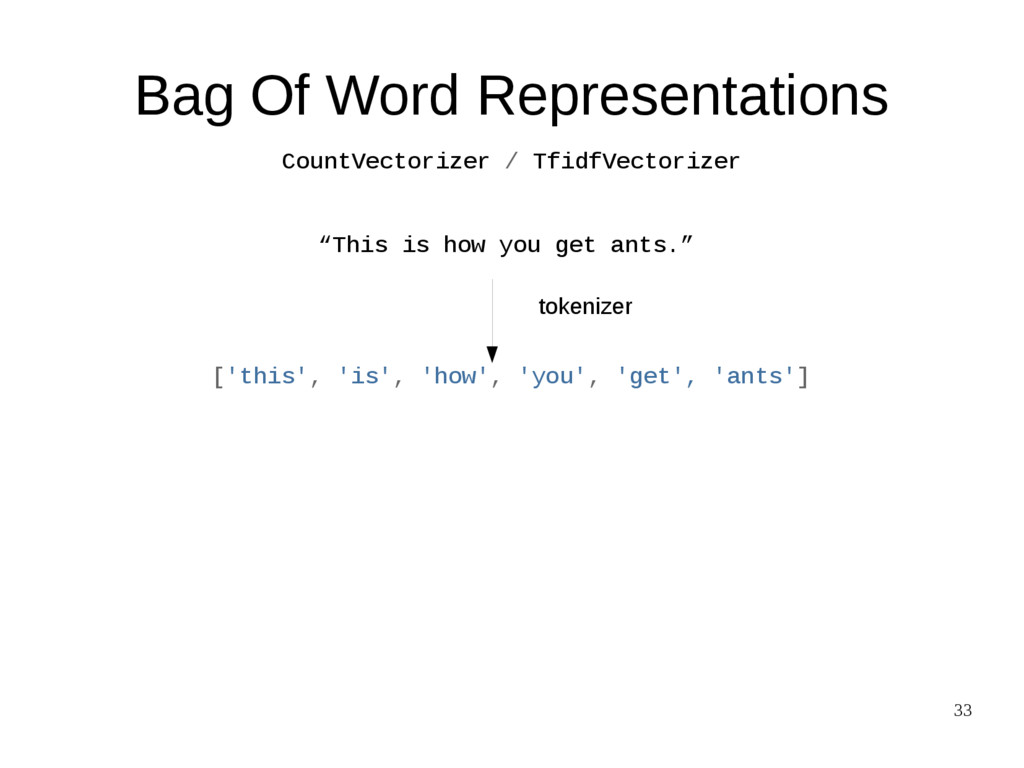
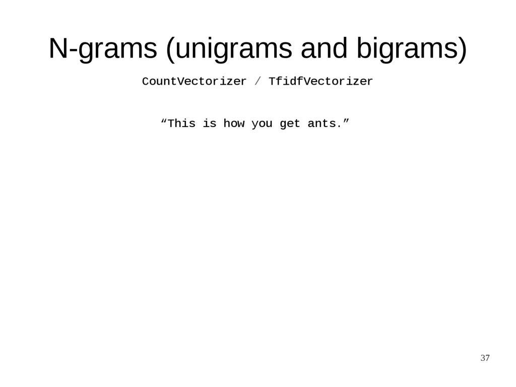
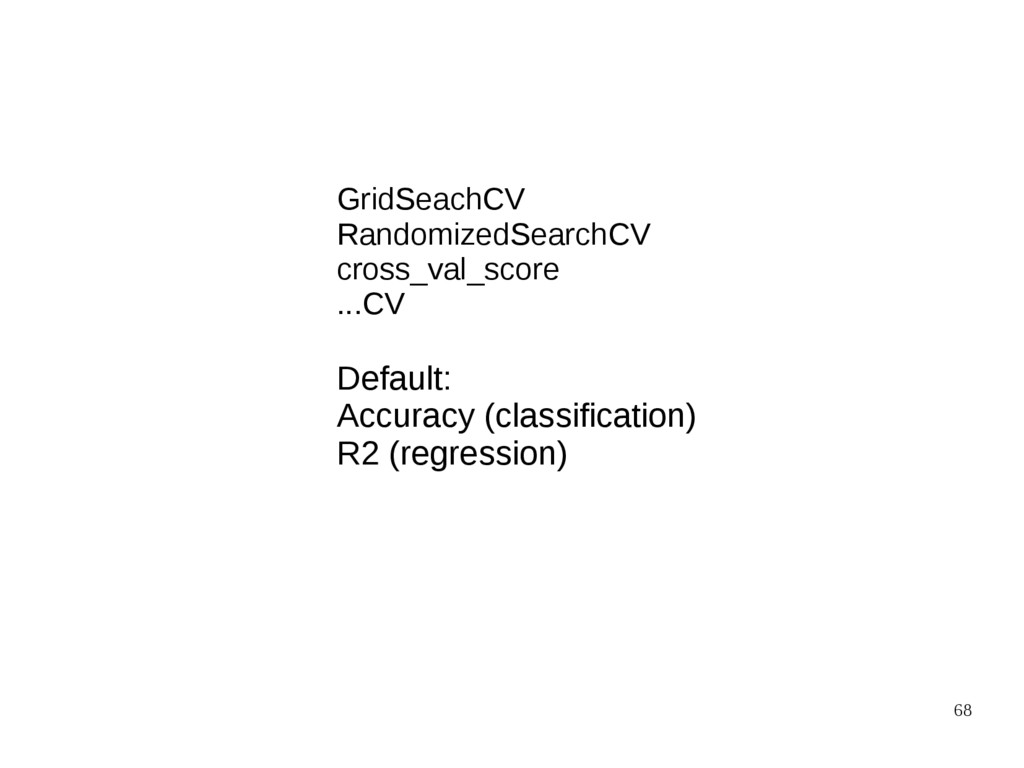
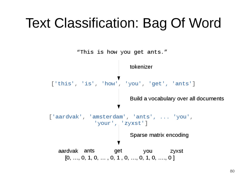
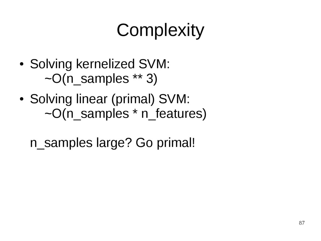
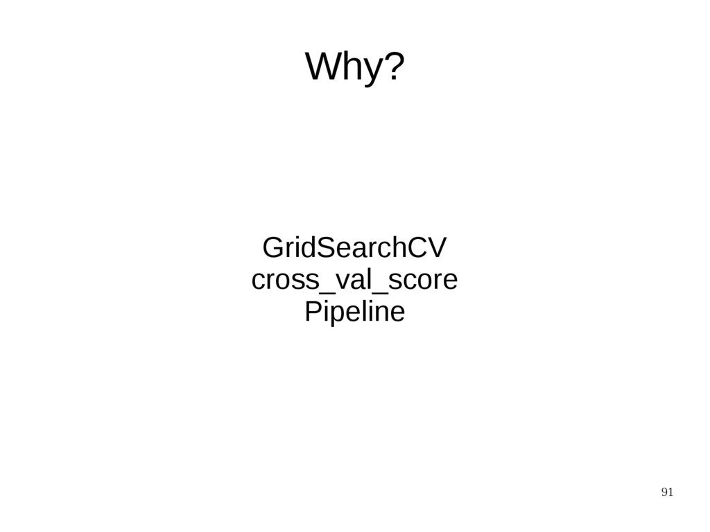
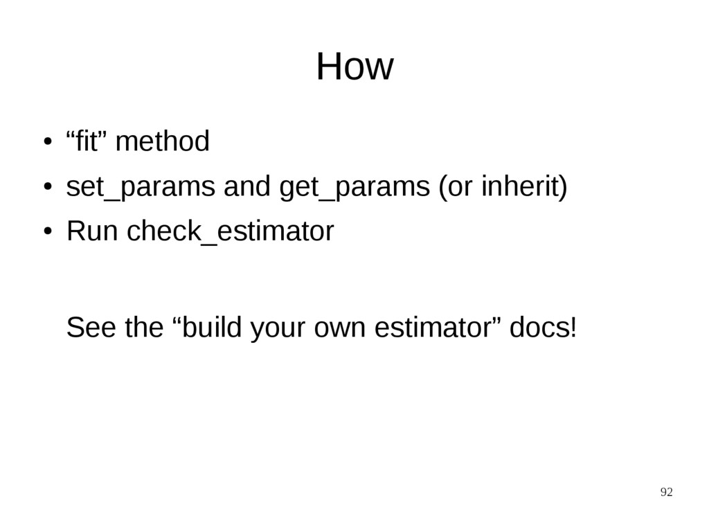
ants.” [0, …, 0, 1, 0, … , 0, 1 , 0, …, 0, 1, 0, …., 0 ] ['this', 'is', 'how', 'you', 'get', 'ants'] tokenizer Sparse matrix encoding hashing [hash('this'), hash('is'), hash('how'), hash('you'), hash('get'), hash('ants')] = [832412, 223788, 366226, 81185, 835749, 173092]
![16 Basic API estimator.fit(X, [y]) estimator.predict estimator.transform Classification Preprocessing Regression](https://files.speakerdeck.com/presentations/9ba7b3621c944f499573898a3991966e/slide_15.jpg)
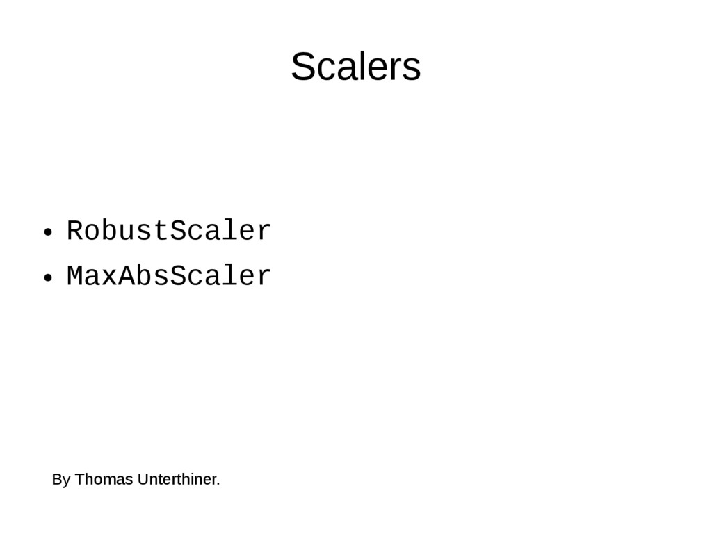
![65 Linear Models Feature Selection Tree-Based models [possible] LogisticRegressionCV [new]](https://files.speakerdeck.com/presentations/9ba7b3621c944f499573898a3991966e/slide_64.jpg)
![111 Thank you! @amuellerml @amueller [email protected] http://amueller.github.io](https://files.speakerdeck.com/presentations/9ba7b3621c944f499573898a3991966e/slide_110.jpg)