Deep Learning Tutorial at ICML 2013 by Yann LeCun and Marc'Aurelio Ranzato

from http://www.cs.nyu.edu/~yann/talks/lecun-ranzato-icml2013.pdf

Transcript

1. Y LeCun MA Ranzato Deep Learning Tutorial ICML, Atlanta, 2013-06-16 Yann LeCun Center for Data Science & Courant Institute, NYU yann@cs.nyu.edu http://yann.lecun.com Marc'Aurelio Ranzato Google ranzato@google.com http://www.cs.toronto.edu/~ranzato
2. Y LeCun MA Ranzato Deep Learning = Learning Representations/Features The traditional model of pattern recognition (since the late 50's) Fixed/engineered features (or fixed kernel) + trainable classifier End-to-end learning / Feature learning / Deep learning Trainable features (or kernel) + trainable classifier “Simple” Trainable Classifier hand-crafted Feature Extractor Trainable Classifier Trainable Feature Extractor
3. Y LeCun MA Ranzato This Basic Model has not evolved much since the 50's The first learning machine: the Perceptron Built at Cornell in 1960 The Perceptron was a linear classifier on top of a simple feature extractor The vast majority of practical applications of ML today use glorified linear classifiers or glorified template matching. Designing a feature extractor requires considerable efforts by experts. y=sign (∑ i=1 N W i F i ( X )+b ) A Feature Extractor Wi
4. Y LeCun MA Ranzato Architecture of “Mainstream”Pattern Recognition Systems Modern architecture for pattern recognition Speech recognition: early 90's – 2011 Object Recognition: 2006 - 2012 fixed unsupervised supervised Classifier MFCC Mix of Gaussians Classifier SIFT HoG K-means Sparse Coding Pooling fixed unsupervised supervised Low-level Features Mid-level Features
5. Y LeCun MA Ranzato Deep Learning = Learning Hierarchical Representations It's deep if it has more than one stage of non-linear feature transformation Trainable Classifier Low-Level Feature Mid-Level Feature High-Level Feature Feature visualization of convolutional net trained on ImageNet from [Zeiler & Fergus 2013]
6. Y LeCun MA Ranzato Trainable Feature Hierarchy Hierarchy of representations with increasing level of abstraction Each stage is a kind of trainable feature transform Image recognition Pixel edge texton motif part object → → → → → Text Character word word group clause sentence story → → → → → Speech Sample spectral band sound … phone phoneme → → → → → → word →
7. Y LeCun MA Ranzato Learning Representations: a challenge for ML, CV, AI, Neuroscience, Cognitive Science... How do we learn representations of the perceptual world? How can a perceptual system build itself by looking at the world? How much prior structure is necessary ML/AI: how do we learn features or feature hierarchies? What is the fundamental principle? What is the learning algorithm? What is the architecture? Neuroscience: how does the cortex learn perception? Does the cortex “run” a single, general learning algorithm? (or a small number of them) CogSci: how does the mind learn abstract concepts on top of less abstract ones? Deep Learning addresses the problem of learning hierarchical representations with a single algorithm Trainable Feature Transform Trainable Feature Transform Trainable Feature Transform Trainable Feature Transform
8. Y LeCun MA Ranzato The Mammalian Visual Cortex is Hierarchical [picture from Simon Thorpe] [Gallant & Van Essen] The ventral (recognition) pathway in the visual cortex has multiple stages Retina - LGN - V1 - V2 - V4 - PIT - AIT .... Lots of intermediate representations
9. Y LeCun MA Ranzato Let's be inspired by nature, but not too much It's nice imitate Nature, But we also need to understand How do we know which details are important? Which details are merely the result of evolution, and the constraints of biochemistry? For airplanes, we developed aerodynamics and compressible fluid dynamics. We figured that feathers and wing flapping weren't crucial QUESTION: What is the equivalent of aerodynamics for understanding intelligence? L'Avion III de Clément Ader, 1897 (Musée du CNAM, Paris) His Eole took off from the ground in 1890, 13 years before the Wright Brothers, but you probably never heard of it.
10. Y LeCun MA Ranzato Trainable Feature Hierarchies: End-to-end learning A hierarchy of trainable feature transforms Each module transforms its input representation into a higher-level one. High-level features are more global and more invariant Low-level features are shared among categories Trainable Feature Transform Trainable Feature Transform Trainable Classifier/ Predictor Learned Internal Representations How can we make all the modules trainable and get them to learn appropriate representations?
11. Y LeCun MA Ranzato Three Types of Deep Architectures Feed-Forward: multilayer neural nets, convolutional nets Feed-Back: Stacked Sparse Coding, Deconvolutional Nets Bi-Drectional: Deep Boltzmann Machines, Stacked Auto-Encoders
12. Y LeCun MA Ranzato Three Types of Training Protocols Purely Supervised Initialize parameters randomly Train in supervised mode typically with SGD, using backprop to compute gradients Used in most practical systems for speech and image recognition Unsupervised, layerwise + supervised classifier on top Train each layer unsupervised, one after the other Train a supervised classifier on top, keeping the other layers fixed Good when very few labeled samples are available Unsupervised, layerwise + global supervised fine-tuning Train each layer unsupervised, one after the other Add a classifier layer, and retrain the whole thing supervised Good when label set is poor (e.g. pedestrian detection) Unsupervised pre-training often uses regularized auto-encoders
13. Y LeCun MA Ranzato Do we really need deep architectures? Theoretician's dilemma: “We can approximate any function as close as we want with shallow architecture. Why would we need deep ones?” kernel machines (and 2-layer neural nets) are “universal”. Deep learning machines Deep machines are more efficient for representing certain classes of functions, particularly those involved in visual recognition they can represent more complex functions with less “hardware” We need an efficient parameterization of the class of functions that are useful for “AI” tasks (vision, audition, NLP...)
14. Y LeCun MA Ranzato Why would deep architectures be more efficient? A deep architecture trades space for time (or breadth for depth) more layers (more sequential computation), but less hardware (less parallel computation). Example1: N-bit parity requires N-1 XOR gates in a tree of depth log(N). Even easier if we use threshold gates requires an exponential number of gates of we restrict ourselves to 2 layers (DNF formula with exponential number of minterms). Example2: circuit for addition of 2 N-bit binary numbers Requires O(N) gates, and O(N) layers using N one-bit adders with ripple carry propagation. Requires lots of gates (some polynomial in N) if we restrict ourselves to two layers (e.g. Disjunctive Normal Form). Bad news: almost all boolean functions have a DNF formula with an exponential number of minterms O(2^N)..... [Bengio & LeCun 2007 “Scaling Learning Algorithms Towards AI”]
15. Y LeCun MA Ranzato Which Models are Deep? 2-layer models are not deep (even if you train the first layer) Because there is no feature hierarchy Neural nets with 1 hidden layer are not deep SVMs and Kernel methods are not deep Layer1: kernels; layer2: linear The first layer is “trained” in with the simplest unsupervised method ever devised: using the samples as templates for the kernel functions. Classification trees are not deep No hierarchy of features. All decisions are made in the input space
16. Y LeCun MA Ranzato Are Graphical Models Deep? There is no opposition between graphical models and deep learning. Many deep learning models are formulated as factor graphs Some graphical models use deep architectures inside their factors Graphical models can be deep (but most are not). Factor Graph: sum of energy functions Over inputs X, outputs Y and latent variables Z. Trainable parameters: W Each energy function can contain a deep network The whole factor graph can be seen as a deep network −log P( X ,Y , Z /W )∝E ( X ,Y , Z ,W )=∑ i E i ( X ,Y ,Z ,W i ) E1(X1,Y1) E2(X2,Z1,Z2) E3(Z2,Y1) E4(Y3,Y4) X1 Z3 Y2 Y1 Z2 Z1 X2
17. Y LeCun MA Ranzato Deep Learning: A Theoretician's Nightmare? Deep Learning involves non-convex loss functions With non-convex losses, all bets are off Then again, every speech recognition system ever deployed has used non-convex optimization (GMMs are non convex). But to some of us all “interesting” learning is non convex Convex learning is invariant to the order in which sample are presented (only depends on asymptotic sample frequencies). Human learning isn't like that: we learn simple concepts before complex ones. The order in which we learn things matter.
18. Y LeCun MA Ranzato Deep Learning: A Theoretician's Nightmare? No generalization bounds? Actually, the usual VC bounds apply: most deep learning systems have a finite VC dimension We don't have tighter bounds than that. But then again, how many bounds are tight enough to be useful for model selection? It's hard to prove anything about deep learning systems Then again, if we only study models for which we can prove things, we wouldn't have speech, handwriting, and visual object recognition systems today.
19. Y LeCun MA Ranzato Deep Learning: A Theoretician's Paradise? Deep Learning is about representing high-dimensional data There has to be interesting theoretical questions there What is the geometry of natural signals? Is there an equivalent of statistical learning theory for unsupervised learning? What are good criteria on which to base unsupervised learning? Deep Learning Systems are a form of latent variable factor graph Internal representations can be viewed as latent variables to be inferred, and deep belief networks are a particular type of latent variable models. The most interesting deep belief nets have intractable loss functions: how do we get around that problem? Lots of theory at the 2012 IPAM summer school on deep learning Wright's parallel SGD methods, Mallat's “scattering transform”, Osher's “split Bregman” methods for sparse modeling, Morton's “algebraic geometry of DBN”,....
20. Y LeCun MA Ranzato Deep Learning and Feature Learning Today Deep Learning has been the hottest topic in speech recognition in the last 2 years A few long-standing performance records were broken with deep learning methods Microsoft and Google have both deployed DL-based speech recognition system in their products Microsoft, Google, IBM, Nuance, AT&T, and all the major academic and industrial players in speech recognition have projects on deep learning Deep Learning is the hottest topic in Computer Vision Feature engineering is the bread-and-butter of a large portion of the CV community, which creates some resistance to feature learning But the record holders on ImageNet and Semantic Segmentation are convolutional nets Deep Learning is becoming hot in Natural Language Processing Deep Learning/Feature Learning in Applied Mathematics The connection with Applied Math is through sparse coding, non-convex optimization, stochastic gradient algorithms, etc...
21. Y LeCun MA Ranzato In Many Fields, Feature Learning Has Caused a Revolution (methods used in commercially deployed systems) Speech Recognition I (late 1980s) Trained mid-level features with Gaussian mixtures (2-layer classifier) Handwriting Recognition and OCR (late 1980s to mid 1990s) Supervised convolutional nets operating on pixels Face & People Detection (early 1990s to mid 2000s) Supervised convolutional nets operating on pixels (YLC 1994, 2004, Garcia 2004) Haar features generation/selection (Viola-Jones 2001) Object Recognition I (mid-to-late 2000s: Ponce, Schmid, Yu, YLC....) Trainable mid-level features (K-means or sparse coding) Low-Res Object Recognition: road signs, house numbers (early 2010's) Supervised convolutional net operating on pixels Speech Recognition II (circa 2011) Deep neural nets for acoustic modeling Object Recognition III, Semantic Labeling (2012, Hinton, YLC,...) Supervised convolutional nets operating on pixels
22. Y LeCun MA Ranzato D-AE DBN DBM AE Perceptron RBM GMM BayesNP SVM Sparse Coding  DecisionTree Boosting SHALLOW DEEP Conv. Net Neural Net RNN
23. Y LeCun MA Ranzato SHALLOW DEEP Neural Networks Probabilistic Models D-AE DBN DBM AE Perceptron RBM GMM BayesNP SVM Sparse Coding  DecisionTree Boosting Conv. Net Neural Net RNN
24. Y LeCun MA Ranzato SHALLOW DEEP Neural Networks Probabilistic Models Conv. Net D-AE DBN DBM AE Perceptron RBM GMM BayesNP SVM Supervised Supervised Unsupervised Sparse Coding  Boosting DecisionTree Neural Net RNN
25. Y LeCun MA Ranzato SHALLOW DEEP D-AE DBN DBM AE Perceptro n RBM GMM BayesNP SVM Sparse Coding  Boosting DecisionTree Neural Net Conv. Net RNN In this talk, we'll focus on the simplest and typically most effective methods.
26. Y LeCun MA Ranzato What Are Good Feature?
27. Y LeCun MA Ranzato Discovering the Hidden Structure in High-Dimensional Data The manifold hypothesis Learning Representations of Data: Discovering & disentangling the independent explanatory factors The Manifold Hypothesis: Natural data lives in a low-dimensional (non-linear) manifold Because variables in natural data are mutually dependent
28. Y LeCun MA Ranzato Discovering the Hidden Structure in High-Dimensional Data Example: all face images of a person 1000x1000 pixels = 1,000,000 dimensions But the face has 3 cartesian coordinates and 3 Euler angles And humans have less than about 50 muscles in the face Hence the manifold of face images for a person has <56 dimensions The perfect representations of a face image: Its coordinates on the face manifold Its coordinates away from the manifold We do not have good and general methods to learn functions that turns an image into this kind of representation Ideal Feature Extractor [1.2 −3 0.2 −2... ] Face/not face Pose Lighting Expression -----
29. Y LeCun MA Ranzato Disentangling factors of variation The Ideal Disentangling Feature Extractor Pixel 1 Pixel 2 Pixel n Expression View Ideal Feature Extractor
30. Y LeCun MA Ranzato Data Manifold & Invariance: Some variations must be eliminated Azimuth-Elevation manifold. Ignores lighting. [Hadsell et al. CVPR 2006]
31. Y LeCun MA Ranzato Basic Idea fpr Invariant Feature Learning Embed the input non-linearly into a high(er) dimensional space In the new space, things that were non separable may become separable Pool regions of the new space together Bringing together things that are semantically similar. Like pooling. Non-Linear Function Pooling Or Aggregation Input high-dim Unstable/non-smooth features Stable/invariant features
32. Y LeCun MA Ranzato Non-Linear Expansion → Pooling Entangled data manifolds Non-Linear Dim Expansion, Disentangling Pooling. Aggregation
33. Y LeCun MA Ranzato Sparse Non-Linear Expansion → Pooling Use clustering to break things apart, pool together similar things Clustering, Quantization, Sparse Coding Pooling. Aggregation
34. Y LeCun MA Ranzato Overall Architecture: Normalization → Filter Bank → Non-Linearity → Pooling Stacking multiple stages of [Normalization Filter Bank Non-Linearity Pooling]. → → → Normalization: variations on whitening Subtractive: average removal, high pass filtering Divisive: local contrast normalization, variance normalization Filter Bank: dimension expansion, projection on overcomplete basis Non-Linearity: sparsification, saturation, lateral inhibition.... Rectification (ReLU), Component-wise shrinkage, tanh, winner-takes-all Pooling: aggregation over space or feature type X i ; L p : p √X i p ; PROB: 1 b log (∑ i ebX i ) Classifier feature Pooling Non- Linear Filter Bank Norm feature Pooling Non- Linear Filter Bank Norm
35. Y LeCun MA Ranzato Deep Supervised Learning (modular approach)
36. Y LeCun MA Ranzato Multimodule Systems: Cascade Complex learning machines can be built by assembling modules into networks Simple example: sequential/layered feed-forward architecture (cascade) Forward Propagation:
37. Y LeCun MA Ranzato Multimodule Systems: Implementation Each module is an object Contains trainable parameters Inputs are arguments Output is returned, but also stored internally Example: 2 modules m1, m2 Torch7 (by hand) hid = m1:forward(in) out = m2:forward(hid) Torch7 (using the nn.Sequential class) model = nn.Sequential() model:add(m1) model:add(m2) out = model:forward(in)
38. Y LeCun MA Ranzato Computing the Gradient in Multi-Layer Systems
39. Y LeCun MA Ranzato Computing the Gradient in Multi-Layer Systems
40. Y LeCun MA Ranzato Computing the Gradient in Multi-Layer Systems
41. Y LeCun MA Ranzato Jacobians and Dimensions
42. Y LeCun MA Ranzato Back Propgation
43. Y LeCun MA Ranzato Multimodule Systems: Implementation Backpropagation through a module Contains trainable parameters Inputs are arguments Gradient with respect to input is returned. Arguments are input and gradient with respect to output Torch7 (by hand) hidg = m2:backward(hid,outg) ing = m1:backward(in,hidg) Torch7 (using the nn.Sequential class) ing = model:backward(in,outg)
44. Y LeCun MA Ranzato Linear Module
45. Y LeCun MA Ranzato Tanh module (or any other pointwise function)
46. Y LeCun MA Ranzato Euclidean Distance Module
47. Y LeCun MA Ranzato Any Architecture works Any connection is permissible Networks with loops must be “unfolded in time”. Any module is permissible As long as it is continuous and differentiable almost everywhere with respect to the parameters, and with respect to non-terminal inputs.
48. Y LeCun MA Ranzato Module-Based Deep Learning with Torch7 Torch7 is based on the Lua language Simple and lightweight scripting language, dominant in the game industry Has a native just-in-time compiler (fast!) Has a simple foreign function interface to call C/C++ functions from Lua Torch7 is an extension of Lua with A multidimensional array engine with CUDA and OpenMP backends A machine learning library that implements multilayer nets, convolutional nets, unsupervised pre-training, etc Various libraries for data/image manipulation and computer vision A quickly growing community of users Single-line installation on Ubuntu and Mac OSX: curl -s https://raw.github.com/clementfarabet/torchinstall/master/install | bash Torch7 Machine Learning Tutorial (neural net, convnet, sparse auto-encoder): http://code.cogbits.com/wiki/doku.php
49. Y LeCun MA Ranzato Example: building a Neural Net in Torch7 Net for SVHN digit recognition 10 categories Input is 32x32 RGB (3 channels) 1500 hidden units Creating a 2-layer net Make a cascade module Reshape input to vector Add Linear module Add tanh module Add Linear Module Add log softmax layer Create loss function module Noutputs = 10; nfeats = 3; Width = 32; height = 32 ninputs = nfeats*width*height nhiddens = 1500 ­­ Simple 2­layer neural network model = nn.Sequential() model:add(nn.Reshape(ninputs)) model:add(nn.Linear(ninputs,nhiddens)) model:add(nn.Tanh()) model:add(nn.Linear(nhiddens,noutputs)) model:add(nn.LogSoftMax()) criterion = nn.ClassNLLCriterion() See Torch7 example at http://bit.ly/16tyLAx
50. Y LeCun MA Ranzato Example: Training a Neural Net in Torch7 one epoch over training set Get next batch of samples Create a “closure” feval(x) that takes the parameter vector as argument and returns the loss and its gradient on the batch. Run model on batch backprop Normalize by size of batch Return loss and gradient call the stochastic gradient optimizer for t = 1,trainData:size(),batchSize do inputs,outputs = getNextBatch() local feval = function(x) parameters:copy(x) gradParameters:zero() local f = 0 for i = 1,#inputs do local output = model:forward(inputs[i]) local err = criterion:forward(output,targets[i]) f = f + err local df_do = criterion:backward(output,targets[i]) model:backward(inputs[i], df_do) end gradParameters:div(#inputs) f = f/#inputs return f,gradParameters end – of feval optim.sgd(feval,parameters,optimState) end
51. Y LeCun MA Ranzato % F-PROP for i = 1 : nr_layers - 1 [h{i} jac{i}] = nonlinearity(W{i} * h{i-1} + b{i}); end h{nr_layers-1} = W{nr_layers-1} * h{nr_layers-2} + b{nr_layers-1}; prediction = softmax(h{l-1}); % CROSS ENTROPY LOSS loss = - sum(sum(log(prediction) .* target)) / batch_size; % B-PROP dh{l-1} = prediction - target; for i = nr_layers – 1 : -1 : 1 Wgrad{i} = dh{i} * h{i-1}'; bgrad{i} = sum(dh{i}, 2); dh{i-1} = (W{i}' * dh{i}) .* jac{i-1}; end % UPDATE for i = 1 : nr_layers - 1 W{i} = W{i} – (lr / batch_size) * Wgrad{i}; b{i} = b{i} – (lr / batch_size) * bgrad{i}; end Toy Code (Matlab): Neural Net Trainer
52. Y LeCun MA Ranzato Deep Supervised Learning is Non-Convex Example: what is the loss function for the simplest 2-layer neural net ever Function: 1-1-1 neural net. Map 0.5 to 0.5 and -0.5 to -0.5 (identity function) with quadratic cost:
53. Y LeCun MA Ranzato Backprop in Practice Use ReLU non-linearities (tanh and logistic are falling out of favor) Use cross-entropy loss for classification Use Stochastic Gradient Descent on minibatches Shuffle the training samples Normalize the input variables (zero mean, unit variance) Schedule to decrease the learning rate Use a bit of L1 or L2 regularization on the weights (or a combination) But it's best to turn it on after a couple of epochs Use “dropout” for regularization Hinton et al 2012 http://arxiv.org/abs/1207.0580 Lots more in [LeCun et al. “Efficient Backprop” 1998] Lots, lots more in “Neural Networks, Tricks of the Trade” (2012 edition) edited by G. Montavon, G. B. Orr, and K-R Müller (Springer)
54. Y LeCun MA Ranzato Deep Learning In Speech Recognition
55. Y LeCun MA Ranzato Case study #1: Acoustic Modeling A typical speech recognition system: Feature Extraction Neural Network Decoder Transducer & Language Model Hi, how are you?
56. Y LeCun MA Ranzato Case study #1: Acoustic Modeling A typical speech recognition system: Feature Extraction Neural Network Decoder Transducer & Language Model Hi, how are you? Here, we focus only on the prediction of phone states from short time-windows of spectrogram. For simplicity, we will use a fully connected neural network (in practice, a convolutional net does better). Mohamed et al. “DBNs for phone recognition” NIPS Workshop 2009 Zeiler et al. “On rectified linear units for speech recognition” ICASSP 2013
57. Y LeCun MA Ranzato Data US English: Voice Search, Voice Typing, Read data Billions of training samples Input: log-energy filter bank outputs 40 frequency bands 26 input frames Output: 8000 phone states Zeiler et al. “On rectified linear units for speech recognition” ICASSP 2013
58. Y LeCun MA Ranzato Architecture From 1 to 12 hidden layers For simplicity, the same number of hidden units at each layer: 1040 → 2560 → 2560 → … → 2560 → 8000 Non-linearities: __/ output = max(0, input) Zeiler et al. “On rectified linear units for speech recognition” ICASSP 2013
59. Y LeCun MA Ranzato Energy & Loss Since it is a standard classification problem, the energy is: Zeiler et al. “On rectified linear units for speech recognition” ICASSP 2013 E x , y=−y f  x y 1-of-N vector The loss is the negative log-likelihood: L=E x , ylog∑  y exp−E x ,  y
60. Y LeCun MA Ranzato Optimization SGD with schedule on learning rate Zeiler et al. “On rectified linear units for speech recognition” ICASSP 2013 t t−1 −t ∂ L ∂  t−1 t =  max1, t T  Mini-batches of size 40 Asynchronous SGD (using 100 copies of the network on a few hundred machines). This speeds up training at Google but it is not crucial.
61. Y LeCun MA Ranzato Training Given an input mini-batch FPROP max 0,W 1 x max 0,W 2 h 1  max 0,W n h n−1  Negative Log-Likelihood label y
62. Y LeCun MA Ranzato Training Given an input mini-batch FPROP max 0,W 1 x max 0,W 2 h 1  max 0,W n h n−1  Negative Log-Likelihood label y h 2 = f x ;W 1 
63. Y LeCun MA Ranzato Training Given an input mini-batch FPROP max 0,W 1 x max 0,W 2 h 1  max 0,W n h n−1  Negative Log-Likelihood label y h 2 = f h 1 ;W 2 
64. Y LeCun MA Ranzato Training Given an input mini-batch FPROP max 0,W 1 x max 0,W 2 h 1  max 0,W n h n−1  Negative Log-Likelihood label y h n = f h n−1 
65. Y LeCun MA Ranzato Training Given an input mini-batch FPROP max 0,W 1 x max 0,W 2 h 1  max 0,W n h n−1  Negative Log-Likelihood label y
66. Y LeCun MA Ranzato Training Given an input mini-batch BPROP max 0,W 1 x max 0,W 2 h 1  max 0,W n h n−1  Negative Log-Likelihood label y ∂ L ∂ h n−1 = ∂ L ∂ h n ∂ h n ∂ h n−1 ∂ L ∂W n = ∂ L ∂ h n ∂ h n ∂ W n
67. Y LeCun MA Ranzato Training Given an input mini-batch max 0,W 1 x max 0,W 2 h 1  max 0,W n h n−1  Negative Log-Likelihood label y BPROP ∂ L ∂ h 1 = ∂ L ∂ h 2 ∂ h 2 ∂ h 1 ∂ L ∂W 2 = ∂ L ∂ h 2 ∂ h 2 ∂W 2
68. Y LeCun MA Ranzato Training Given an input mini-batch max 0,W 1 x max 0,W 2 h 1  max 0,W n h n−1  Negative Log-Likelihood label y BPROP ∂ L ∂W 1 = ∂ L ∂ h 1 ∂ h 1 ∂W 1
69. Y LeCun MA Ranzato Training Given an input mini-batch max 0,W 1 x max 0,W 2 h 1  max 0,W n h n−1  Negative Log-Likelihood label y Parameter update  − ∂ L ∂
70. Y LeCun MA Ranzato Training
71. Y LeCun MA Ranzato Zeiler et al. “On rectified linear units for speech recognition” ICASSP 2013 Number of hidden layers Word Error Rate % 1 2 4 8 12 16 12.8 11.4 10.9 11.1 GMM baseline: 15.4% Word Error Rate
72. Y LeCun MA Ranzato Convolutional Networks
73. Y LeCun MA Ranzato Convolutional Nets Are deployed in many practical applications Image recognition, speech recognition, Google's and Baidu's photo taggers Have won several competitions ImageNet, Kaggle Facial Expression, Kaggle Multimodal Learning, German Traffic Signs, Connectomics, Handwriting.... Are applicable to array data where nearby values are correlated Images, sound, time-frequency representations, video, volumetric images, RGB-Depth images,..... One of the few models that can be trained purely supervised input 83x83 Layer 1 64x75x7 5 Layer 2 64@14x14 Layer 3 256@6x6 Layer 4 256@1x1 Output 101 9x9 convolution (64 kernels) 9x9 convolution (4096 kernels) 10x10 pooling, 5x5 subsampling 6x6 pooling 4x4 subsamp
74. Y LeCun MA Ranzato Fully-connected neural net in high dimension Example: 200x200 image Fully-connected, 400,000 hidden units = 16 billion parameters Locally-connected, 400,000 hidden units 10x10 fields = 40 million params Local connections capture local dependencies
75. Y LeCun MA Ranzato Shared Weights & Convolutions: Exploiting Stationarity Features that are useful on one part of the image and probably useful elsewhere. All units share the same set of weights Shift equivariant processing: When the input shifts, the output also shifts but stays otherwise unchanged. Convolution with a learned kernel (or filter) Non-linearity: ReLU (rectified linear) The filtered “image” Z is called a feature map A ij =∑ kl W kl X i+ j. k+l Z ij =max(0, A ij ) Example: 200x200 image 400,000 hidden units with 10x10 fields = 1000 params 10 feature maps of size 200x200, 10 filters of size 10x10
76. Y LeCun MA Ranzato Multiple Convolutions with Different Kernels Detects multiple motifs at each location The collection of units looking at the same patch is akin to a feature vector for that patch. The result is a 3D array, where each slice is a feature map. Multiple convolutions
77. Y LeCun MA Ranzato Early Hierarchical Feature Models for Vision [Hubel & Wiesel 1962]: simple cells detect local features complex cells “pool” the outputs of simple cells within a retinotopic neighborhood. Cognitron & Neocognitron [Fukushima 1974-1982] pooling subsampling “Simple cells” “Complex cells” Multiple convolutions
78. Y LeCun MA Ranzato The Convolutional Net Model (Multistage Hubel-Wiesel system) pooling subsampling “Simple cells” “Complex cells” Multiple convolutions Retinotopic Feature Maps [LeCun et al. 89] [LeCun et al. 98] Training is supervised With stochastic gradient descent
79. Y LeCun MA Ranzato Feature Transform: Normalization → Filter Bank → Non-Linearity → Pooling Stacking multiple stages of [Normalization Filter Bank Non-Linearity Pooling]. → → → Normalization: variations on whitening Subtractive: average removal, high pass filtering Divisive: local contrast normalization, variance normalization Filter Bank: dimension expansion, projection on overcomplete basis Non-Linearity: sparsification, saturation, lateral inhibition.... Rectification, Component-wise shrinkage, tanh, winner-takes-all Pooling: aggregation over space or feature type, subsampling X i ; L p : p √X i p ; PROB: 1 b log (∑ i ebX i ) Classifier feature Pooling Non- Linear Filter Bank Norm feature Pooling Non- Linear Filter Bank Norm
80. Y LeCun MA Ranzato Feature Transform: Normalization → Filter Bank → Non-Linearity → Pooling Filter Bank → Non-Linearity = Non-linear embedding in high dimension Feature Pooling = contraction, dimensionality reduction, smoothing Learning the filter banks at every stage Creating a hierarchy of features Basic elements are inspired by models of the visual (and auditory) cortex Simple Cell + Complex Cell model of [Hubel and Wiesel 1962] Many “traditional” feature extraction methods are based on this SIFT, GIST, HoG, SURF... [Fukushima 1974-1982], [LeCun 1988-now], since the mid 2000: Hinton, Seung, Poggio, Ng,.... Classifier feature Pooling Non- Linear Filter Bank Norm feature Pooling Non- Linear Filter Bank Norm
81. Y LeCun MA Ranzato Convolutional Network (ConvNet) Non-Linearity: half-wave rectification, shrinkage function, sigmoid Pooling: average, L1, L2, max Training: Supervised (1988-2006), Unsupervised+Supervised (2006-now) input 83x83 Layer 1 64x75x75 Layer 2 64@14x14 Layer 3 256@6x6 Layer 4 256@1x1 Output 101 9x9 convolution (64 kernels) 9x9 convolution (4096 kernels) 10x10 pooling, 5x5 subsampling 6x6 pooling 4x4 subsamp
82. Y LeCun MA Ranzato Convolutional Network Architecture
83. Y LeCun MA Ranzato Convolutional Network (vintage 1990) filters → tanh → average-tanh → filters → tanh → average-tanh → filters → tanh Curved manifold Flatter manifold
84. Y LeCun MA Ranzato “Mainstream” object recognition pipeline 2006-2012: somewhat similar to ConvNets Fixed Features + unsupervised mid-level features + simple classifier SIFT + Vector Quantization + Pyramid pooling + SVM [Lazebnik et al. CVPR 2006] SIFT + Local Sparse Coding Macrofeatures + Pyramid pooling + SVM [Boureau et al. ICCV 2011] SIFT + Fisher Vectors + Deformable Parts Pooling + SVM [Perronin et al. 2012] Oriented Edges Winner Takes All Histogram (sum) Filter Bank feature Pooling Non- Linearity Filter Bank feature Pooling Non- Linearity Classifier Fixed (SIFT/HoG/...) K-means Sparse Coding Spatial Max Or average Any simple classifier Unsupervised Supervised
85. Y LeCun MA Ranzato Tasks for Which Deep Convolutional Nets are the Best Handwriting recognition MNIST (many), Arabic HWX (IDSIA) OCR in the Wild [2011]: StreetView House Numbers (NYU and others) Traffic sign recognition [2011] GTSRB competition (IDSIA, NYU) Pedestrian Detection [2013]: INRIA datasets and others (NYU) Volumetric brain image segmentation [2009] connectomics (IDSIA, MIT) Human Action Recognition [2011] Hollywood II dataset (Stanford) Object Recognition [2012] ImageNet competition Scene Parsing [2012] Stanford bgd, SiftFlow, Barcelona (NYU) Scene parsing from depth images [2013] NYU RGB-D dataset (NYU) Speech Recognition [2012] Acoustic modeling (IBM and Google) Breast cancer cell mitosis detection [2011] MITOS (IDSIA) The list of perceptual tasks for which ConvNets hold the record is growing. Most of these tasks (but not all) use purely supervised convnets.
86. Y LeCun MA Ranzato Ideas from Neuroscience and Psychophysics The whole architecture: simple cells and complex cells Local receptive fields Self-similar receptive fields over the visual field (convolutions) Pooling (complex cells) Non-Linearity: Rectified Linear Units (ReLU) LGN-like band-pass filtering and contrast normalization in the input Divisive contrast normalization (from Heeger, Simoncelli....) Lateral inhibition Sparse/Overcomplete representations (Olshausen-Field....) Inference of sparse representations with lateral inhibition Sub-sampling ratios in the visual cortex between 2 and 3 between V1-V2-V4 Crowding and visual metamers give cues on the size of the pooling areas
87. Y LeCun MA Ranzato Simple ConvNet Applications with State-of-the-Art Performance Traffic Sign Recognition (GTSRB) German Traffic Sign Reco Bench 99.2% accuracy #1: IDSIA; #2 NYU House Number Recognition (Google) Street View House Numbers 94.3 % accuracy
88. Y LeCun MA Ranzato Prediction of Epilepsy Seizures from Intra-Cranial EEG Piotr Mirowski, Deepak Mahdevan (NYU Neurology), Yann LeCun
89. Y LeCun MA Ranzato Epilepsy Prediction 4 64 10 32 … … … … … … … … … … … 32 … … … … … 8 32 384 feature extraction over short time windows for individual channels (we look for 10 sorts of features) integration of all channels and all features across several time samples EEG channels time, in samples … integration of all channels and all features across several time samples inputs outputs Temporal Convolutional Net
90. Y LeCun MA Ranzato ConvNet in Connectomics [Jain, Turaga, Seung 2007-present] 3D convnet to segment volumetric images
91. Y LeCun MA Ranzato Object Recognition [Krizhevsky, Sutskever, Hinton 2012] CONV 11x11/ReLU 96fm LOCAL CONTRAST NORM MAX POOL 2x2sub FULL 4096/ReLU FULL CONNECT CONV 11x11/ReLU 256fm LOCAL CONTRAST NORM MAX POOLING 2x2sub CONV 3x3/ReLU 384fm CONV 3x3ReLU 384fm CONV 3x3/ReLU 256fm MAX POOLING FULL 4096/ReLU Won the 2012 ImageNet LSVRC. 60 Million parameters, 832M MAC ops 4M 16M 37M 442K 1.3M 884K 307K 35K 4Mflop 16M 37M 74M 224M 149M 223M 105M
92. Y LeCun MA Ranzato Object Recognition: ILSVRC 2012 results ImageNet Large Scale Visual Recognition Challenge 1000 categories, 1.5 Million labeled training samples
93. Y LeCun MA Ranzato Object Recognition [Krizhevsky, Sutskever, Hinton 2012] Method: large convolutional net 650K neurons, 832M synapses, 60M parameters Trained with backprop on GPU Trained “with all the tricks Yann came up with in the last 20 years, plus dropout” (Hinton, NIPS 2012) Rectification, contrast normalization,... Error rate: 15% (whenever correct class isn't in top 5) Previous state of the art: 25% error A REVOLUTION IN COMPUTER VISION Acquired by Google in Jan 2013 Deployed in Google+ Photo Tagging in May 2013
94. Y LeCun MA Ranzato Object Recognition [Krizhevsky, Sutskever, Hinton 2012]
95. Y LeCun MA Ranzato Object Recognition [Krizhevsky, Sutskever, Hinton 2012] TEST IMAGE RETRIEVED IMAGES
96. Y LeCun MA Ranzato ConvNet-Based Google+ Photo Tagger Searched my personal collection for “bird” Samy Bengio ???
97. Y LeCun MA Ranzato Another ImageNet-trained ConvNet [Zeiler & Fergus 2013] Convolutional Net with 8 layers, input is 224x224 pixels conv-pool-conv-pool-conv-conv-conv-full-full-full Rectified-Linear Units (ReLU): y = max(0,x) Divisive contrast normalization across features [Jarrett et al. ICCV 2009] Trained on ImageNet 2012 training set 1.3M images, 1000 classes 10 different crops/flips per image Regularization: Dropout [Hinton 2012] zeroing random subsets of units Stochastic gradient descent for 70 epochs (7-10 days) With learning rate annealing
98. Y LeCun MA Ranzato Object Recognition on-line demo [Zeiler & Fergus 2013] http://horatio.cs.nyu.edu
99. Y LeCun MA Ranzato ConvNet trained on ImageNet [Zeiler & Fergus 2013]
100. Y LeCun MA Ranzato State of the art with only 6 training examples Features are generic: Caltech 256 Network first trained on ImageNet. Last layer chopped off Last layer trained on Caltech 256, first layers N-1 kept fixed. State of the art accuracy with only 6 training samples/class 3: [Bo, Ren, Fox. CVPR, 2013] 16: [Sohn, Jung, Lee, Hero ICCV 2011]
101. Y LeCun MA Ranzato Features are generic: PASCAL VOC 2012 Network first trained on ImageNet. Last layer trained on Pascal VOC, keeping N-1 first layers fixed. [15] K. Sande, J. Uijlings, C. Snoek, and A. Smeulders. Hybrid coding for selective search. In PASCAL VOC Classification Challenge 2012, [19] S. Yan, J. Dong, Q. Chen, Z. Song, Y. Pan, W. Xia, Z. Huang, Y. Hua, and S. Shen. Generalized hierarchical matching for sub-category aware object classification. In PASCAL VOC Classification Challenge 2012
102. Y LeCun MA Ranzato Semantic Labeling: Labeling every pixel with the object it belongs to [Farabet et al. ICML 2012, PAMI 2013] Would help identify obstacles, targets, landing sites, dangerous areas Would help line up depth map with edge maps
103. Y LeCun MA Ranzato Scene Parsing/Labeling: ConvNet Architecture Each output sees a large input context: 46x46 window at full rez; 92x92 at ½ rez; 184x184 at ¼ rez [7x7conv]->[2x2pool]->[7x7conv]->[2x2pool]->[7x7conv]-> Trained supervised on fully-labeled images Laplacian Pyramid Level 1 Features Level 2 Features Upsampled Level 2 Features Categories
104. Y LeCun MA Ranzato Scene Parsing/Labeling: Performance Stanford Background Dataset [Gould 1009]: 8 categories [Farabet et al. IEEE T. PAMI 2013]
105. Y LeCun MA Ranzato Scene Parsing/Labeling: Performance [Farabet et al. IEEE T. PAMI 2012] SIFT Flow Dataset [Liu 2009]: 33 categories Barcelona dataset [Tighe 2010]: 170 categories.
106. Y LeCun MA Ranzato Scene Parsing/Labeling: SIFT Flow dataset (33 categories) Samples from the SIFT-Flow dataset (Liu) [Farabet et al. ICML 2012, PAMI 2013]
107. Y LeCun MA Ranzato Scene Parsing/Labeling: SIFT Flow dataset (33 categories) [Farabet et al. ICML 2012, PAMI 2013]
108. Y LeCun MA Ranzato Scene Parsing/Labeling [Farabet et al. ICML 2012, PAMI 2013]
109. Y LeCun MA Ranzato Scene Parsing/Labeling [Farabet et al. ICML 2012, PAMI 2013]
110. Y LeCun MA Ranzato Scene Parsing/Labeling [Farabet et al. ICML 2012, PAMI 2013]
111. Y LeCun MA Ranzato Scene Parsing/Labeling [Farabet et al. ICML 2012, PAMI 2013]
112. Y LeCun MA Ranzato Scene Parsing/Labeling No post-processing Frame-by-frame ConvNet runs at 50ms/frame on Virtex-6 FPGA hardware But communicating the features over ethernet limits system performance
113. Y LeCun MA Ranzato Scene Parsing/Labeling: Temporal Consistency Causal method for temporal consistency [Couprie, Farabet, Najman, LeCun ICLR 2013, ICIP 2013]
114. Y LeCun MA Ranzato NYU RGB-Depth Indoor Scenes Dataset 407024 RGB-D images of apartments 1449 labeled frames, 894 object categories [Silberman et al. 2012]
115. Y LeCun MA Ranzato Scene Parsing/Labeling on RGB+Depth Images With temporal consistency [Couprie, Farabet, Najman, LeCun ICLR 2013, ICIP 2013]
116. Y LeCun MA Ranzato Scene Parsing/Labeling on RGB+Depth Images With temporal consistency [Couprie, Farabet, Najman, LeCun ICLR 2013, ICIP 2013]
117. Y LeCun MA Ranzato Semantic Segmentation on RGB+D Images and Videos [Couprie, Farabet, Najman, LeCun ICLR 2013, ICIP 2013]
118. Y LeCun MA Ranzato Energy-Based Unsupervised Learning
119. Y LeCun MA Ranzato Energy-Based Unsupervised Learning Learning an energy function (or contrast function) that takes Low values on the data manifold Higher values everywhere else Y1 Y2
120. Y LeCun MA Ranzato Capturing Dependencies Between Variables with an Energy Function The energy surface is a “contrast function” that takes low values on the data manifold, and higher values everywhere else Special case: energy = negative log density Example: the samples live in the manifold Y1 Y2 Y 2 =(Y 1 )2
121. Y LeCun MA Ranzato Transforming Energies into Probabilities (if necessary) Y P(Y|W) Y E(Y,W) The energy can be interpreted as an unnormalized negative log density Gibbs distribution: Probability proportional to exp(-energy) Beta parameter is akin to an inverse temperature Don't compute probabilities unless you absolutely have to Because the denominator is often intractable
122. Y LeCun MA Ranzato Learning the Energy Function parameterized energy function E(Y,W) Make the energy low on the samples Make the energy higher everywhere else Making the energy low on the samples is easy But how do we make it higher everywhere else?
123. Y LeCun MA Ranzato Seven Strategies to Shape the Energy Function 1. build the machine so that the volume of low energy stuff is constant PCA, K-means, GMM, square ICA 2. push down of the energy of data points, push up everywhere else Max likelihood (needs tractable partition function) 3. push down of the energy of data points, push up on chosen locations contrastive divergence, Ratio Matching, Noise Contrastive Estimation, Minimum Probability Flow 4. minimize the gradient and maximize the curvature around data points score matching 5. train a dynamical system so that the dynamics goes to the manifold denoising auto-encoder 6. use a regularizer that limits the volume of space that has low energy Sparse coding, sparse auto-encoder, PSD 7. if E(Y) = ||Y - G(Y)||^2, make G(Y) as "constant" as possible. Contracting auto-encoder, saturating auto-encoder
124. Y LeCun MA Ranzato #1: constant volume of low energy 1. build the machine so that the volume of low energy stuff is constant PCA, K-means, GMM, square ICA... E(Y )=∥W T WY −Y∥2 PCA K-Means, Z constrained to 1-of-K code E(Y )=min z ∑ i ∥Y −W i Z i ∥2
125. Y LeCun MA Ranzato #2: push down of the energy of data points, push up everywhere else Max likelihood (requires a tractable partition function) Y P(Y) Y E(Y) Maximizing P(Y|W) on training samples make this big make this big make this small Minimizing -log P(Y,W) on training samples make this small
126. Y LeCun MA Ranzato #2: push down of the energy of data points, push up everywhere else Gradient of the negative log-likelihood loss for one sample Y: Pushes down on the energy of the samples Pulls up on the energy of low-energy Y's Y Y E(Y) Gradient descent:
127. Y LeCun MA Ranzato #3. push down of the energy of data points, push up on chosen locations contrastive divergence, Ratio Matching, Noise Contrastive Estimation, Minimum Probability Flow Contrastive divergence: basic idea Pick a training sample, lower the energy at that point From the sample, move down in the energy surface with noise Stop after a while Push up on the energy of the point where we stopped This creates grooves in the energy surface around data manifolds CD can be applied to any energy function (not just RBMs) Persistent CD: use a bunch of “particles” and remember their positions Make them roll down the energy surface with noise Push up on the energy wherever they are Faster than CD RBM E(Y ,Z )=−ZT WY E(Y )=−log ∑ z eZ T WY
128. Y LeCun MA Ranzato #6. use a regularizer that limits the volume of space that has low energy Sparse coding, sparse auto-encoder, Predictive Saprse Decomposition
129. Y LeCun MA Ranzato Sparse Modeling, Sparse Auto-Encoders, Predictive Sparse Decomposition LISTA
130. Y LeCun MA Ranzato How to Speed Up Inference in a Generative Model? Factor Graph with an asymmetric factor Inference Z → Y is easy Run Z through deterministic decoder, and sample Y Inference Y → Z is hard, particularly if Decoder function is many-to-one MAP: minimize sum of two factors with respect to Z Z* = argmin_z Distance[Decoder(Z), Y] + FactorB(Z) Examples: K-Means (1of K), Sparse Coding (sparse), Factor Analysis INPUT Decoder Y Distance Z LATENT VARIABLE Factor B Generative Model Factor A
131. Y LeCun MA Ranzato Sparse Coding & Sparse Modeling Sparse linear reconstruction Energy = reconstruction_error + code_prediction_error + code_sparsity E(Yi ,Z )=∥Yi−W d Z∥2+ λ∑ j ∣z j ∣ [Olshausen & Field 1997] INPUT Y Z ∥Yi−  Y∥2 ∣z j ∣ W d Z FEATURES ∑ j . Y → ̂ Z=argmin Z E(Y ,Z) Inference is slow DETERMINISTIC FUNCTION FACTOR VARIABLE
132. Y LeCun MA Ranzato Encoder Architecture Examples: most ICA models, Product of Experts INPUT Y Z LATENT VARIABLE Factor B Encoder Distance Fast Feed-Forward Model Factor A'
133. Y LeCun MA Ranzato Encoder-Decoder Architecture Train a “simple” feed-forward function to predict the result of a complex optimization on the data points of interest INPUT Decoder Y Distance Z LATENT VARIABLE Factor B [Kavukcuoglu, Ranzato, LeCun, rejected by every conference, 2008-2009] Generative Model Factor A Encoder Distance Fast Feed-Forward Model Factor A' 1. Find optimal Zi for all Yi; 2. Train Encoder to predict Zi from Yi
134. Y LeCun MA Ranzato Why Limit the Information Content of the Code? INPUT SPACE FEATURE SPACE Training sample Input vector which is NOT a training sample Feature vector
135. Y LeCun MA Ranzato Why Limit the Information Content of the Code? INPUT SPACE FEATURE SPACE Training sample Input vector which is NOT a training sample Feature vector Training based on minimizing the reconstruction error over the training set
136. Y LeCun MA Ranzato Why Limit the Information Content of the Code? INPUT SPACE FEATURE SPACE Training sample Input vector which is NOT a training sample Feature vector BAD: machine does not learn structure from training data!! It just copies the data.
137. Y LeCun MA Ranzato Why Limit the Information Content of the Code? Training sample Input vector which is NOT a training sample Feature vector IDEA: reduce number of available codes. INPUT SPACE FEATURE SPACE
138. Y LeCun MA Ranzato Why Limit the Information Content of the Code? Training sample Input vector which is NOT a training sample Feature vector IDEA: reduce number of available codes. INPUT SPACE FEATURE SPACE
139. Y LeCun MA Ranzato Why Limit the Information Content of the Code? Training sample Input vector which is NOT a training sample Feature vector IDEA: reduce number of available codes. INPUT SPACE FEATURE SPACE
140. Y LeCun MA Ranzato Predictive Sparse Decomposition (PSD): sparse auto-encoder Prediction the optimal code with a trained encoder Energy = reconstruction_error + code_prediction_error + code_sparsity EYi ,Z =∥Yi−W d Z∥2∥Z−g e W e ,Yi∥2∑ j ∣z j ∣ g e (W e ,Yi)=shrinkage(W e Yi) [Kavukcuoglu, Ranzato, LeCun, 2008 → arXiv:1010.3467], INPUT Y Z ∥Yi−  Y∥2 ∣z j ∣ W d Z FEATURES ∑ j . ∥Z−  Z∥2 g e W e ,Y i
141. Y LeCun MA Ranzato PSD: Basis Functions on MNIST Basis functions (and encoder matrix) are digit parts
142. Y LeCun MA Ranzato Training on natural images patches. 12X12 256 basis functions Predictive Sparse Decomposition (PSD): Training
143. Y LeCun MA Ranzato Learned Features on natural patches: V1-like receptive fields
144. Y LeCun MA Ranzato ISTA/FISTA: iterative algorithm that converges to optimal sparse code INPUT Y Z W e sh() S + [Gregor & LeCun, ICML 2010], [Bronstein et al. ICML 2012], [Rolfe & LeCun ICLR 2013] Lateral Inhibition Better Idea: Give the “right” structure to the encoder
145. Y LeCun MA Ranzato Think of the FISTA flow graph as a recurrent neural net where We and S are trainable parameters INPUT Y Z W e sh() S + Time-Unfold the flow graph for K iterations Learn the We and S matrices with “backprop-through-time” Get the best approximate solution within K iterations Y Z W e sh() + S sh() + S LISTA: Train We and S matrices to give a good approximation quickly
146. Y LeCun MA Ranzato Learning ISTA (LISTA) vs ISTA/FISTA
147. Y LeCun MA Ranzato LISTA with partial mutual inhibition matrix
148. Y LeCun MA Ranzato Learning Coordinate Descent (LcoD): faster than LISTA
149. Y LeCun MA Ranzato Architecture Rectified linear units Classification loss: cross-entropy Reconstruction loss: squared error Sparsity penalty: L1 norm of last hidden layer Rows of Wd and columns of We constrained in unit sphere W e ()+ S + W c W d Can be repeated Encoding Filters Lateral Inhibition Decoding Filters ̄ X ̄ Y X L 1 ̄ Z X Y 0 ()+ [Rolfe & LeCun ICLR 2013] Discriminative Recurrent Sparse Auto-Encoder (DrSAE)
150. Y LeCun MA Ranzato Image = prototype + sparse sum of “parts” (to move around the manifold) DrSAE Discovers manifold structure of handwritten digits
151. Y LeCun MA Ranzato Replace the dot products with dictionary element by convolutions. Input Y is a full image Each code component Zk is a feature map (an image) Each dictionary element is a convolution kernel Regular sparse coding Convolutional S.C. ∑ k . * Zk Wk Y = “deconvolutional networks” [Zeiler, Taylor, Fergus CVPR 2010] Convolutional Sparse Coding
152. Y LeCun MA Ranzato Convolutional Formulation Extend sparse coding from PATCH to IMAGE PATCH based learning CONVOLUTIONAL learning Convolutional PSD: Encoder with a soft sh() Function
153. Y LeCun MA Ranzato Convolutional Sparse Auto-Encoder on Natural Images Filters and Basis Functions obtained with 1, 2, 4, 8, 16, 32, and 64 filters.
154. Y LeCun MA Ranzato Phase 1: train first layer using PSD FEATURES Y Z ∥Y i− ̃ Y∥2 ∣z j ∣ W d Z λ∑. ∥Z− ̃ Z∥2 g e (W e ,Y i) Using PSD to Train a Hierarchy of Features
155. Y LeCun MA Ranzato Phase 1: train first layer using PSD Phase 2: use encoder + absolute value as feature extractor FEATURES Y ∣z j ∣ g e (W e ,Y i) Using PSD to Train a Hierarchy of Features
156. Y LeCun MA Ranzato Phase 1: train first layer using PSD Phase 2: use encoder + absolute value as feature extractor Phase 3: train the second layer using PSD FEATURES Y ∣z j ∣ g e (W e ,Y i) Y Z ∥Y i− ̃ Y∥2 ∣z j ∣ W d Z λ∑. ∥Z− ̃ Z∥2 g e (W e ,Y i) Using PSD to Train a Hierarchy of Features
157. Y LeCun MA Ranzato Phase 1: train first layer using PSD Phase 2: use encoder + absolute value as feature extractor Phase 3: train the second layer using PSD Phase 4: use encoder + absolute value as 2nd feature extractor FEATURES Y ∣z j ∣ g e (W e ,Y i) ∣z j ∣ g e (W e ,Y i) Using PSD to Train a Hierarchy of Features
158. Y LeCun MA Ranzato Phase 1: train first layer using PSD Phase 2: use encoder + absolute value as feature extractor Phase 3: train the second layer using PSD Phase 4: use encoder + absolute value as 2nd feature extractor Phase 5: train a supervised classifier on top Phase 6 (optional): train the entire system with supervised back-propagation FEATURES Y ∣z j ∣ g e (W e ,Y i) ∣z j ∣ g e (W e ,Y i) classifier Using PSD to Train a Hierarchy of Features
159. Y LeCun MA Ranzato [Osadchy,Miller LeCun JMLR 2007],[Kavukcuoglu et al. NIPS 2010] [Sermanet et al. CVPR 2013] Pedestrian Detection, Face Detection
160. Y LeCun MA Ranzato Feature maps from all stages are pooled/subsampled and sent to the final classification layers Pooled low-level features: good for textures and local motifs High-level features: good for “gestalt” and global shape [Sermanet, Chintala, LeCun CVPR 2013] 7x7 filter+tanh 38 feat maps Input 78x126xYUV L2 Pooling 3x3 2040 9x9 filters+tanh 68 feat maps Av Pooling 2x2 filter+tanh ConvNet Architecture with Multi-Stage Features
161. Y LeCun MA Ranzato [Kavukcuoglu et al. NIPS 2010] [Sermanet et al. ArXiv 2012] ConvNet Color+Skip Supervised ConvNet Color+Skip Unsup+Sup ConvNet B&W Unsup+Sup ConvNet B&W Supervised Pedestrian Detection: INRIA Dataset. Miss rate vs false positives
162. Y LeCun MA Ranzato Results on “Near Scale” Images (>80 pixels tall, no occlusions) Daimler p=217 90 ETH p=8 04 TudBrussels p=508 INRIA p=288
163. Y LeCun MA Ranzato Results on “Reasonable” Images (>50 pixels tall, few occlusions) Daimler p=217 90 ETH p=8 04 TudBrussels p=508 INRIA p=288
164. Y LeCun MA Ranzato 128 stage-1 filters on Y channel. Unsupervised training with convolutional predictive sparse decomposition Unsupervised pre-training with convolutional PSD
165. Y LeCun MA Ranzato Stage 2 filters. Unsupervised training with convolutional predictive sparse decomposition Unsupervised pre-training with convolutional PSD
166. Y LeCun MA Ranzato 96x96 input:120x12 0 output: 3x3 Traditional Detectors/Classifiers must be applied to every location on a large input image, at multiple scales. Convolutional nets can replicated over large images very cheaply. The network is applied to multiple scales spaced by 1.5. Applying a ConvNet on Sliding Windows is Very Cheap!
167. Y LeCun MA Ranzato Computational cost for replicated convolutional net: 96x96 -> 4.6 million multiply-accumulate operations 120x120 -> 8.3 million multiply-accumulate ops 240x240 -> 47.5 million multiply-accumulate ops 480x480 -> 232 million multiply-accumulate ops Computational cost for a non-convolutional detector of the same size, applied every 12 pixels: 96x96 -> 4.6 million multiply-accumulate operations 120x120 -> 42.0 million multiply-accumulate operations 240x240 -> 788.0 million multiply-accumulate ops 480x480 -> 5,083 million multiply-accumulate ops 96x96 window 12 pixel shift 84x84 overlap Building a Detector/Recognizer: Replicated Convolutional Nets
168. Y LeCun MA Ranzato
169. Y LeCun MA Ranzato
170. Y LeCun MA Ranzato Musical Genre Recognition with PSD Feature Input: “Constant Q Transform” over 46.4ms windows (1024 samples) 96 filters, with frequencies spaced every quarter tone (4 octaves) Architecture: Input: sequence of contrast-normalized CQT vectors 1: PSD features, 512 trained filters; shrinkage function → rectification 3: pooling over 5 seconds 4: linear SVM classifier. Pooling of SVM categories over 30 seconds GTZAN Dataset 1000 clips, 30 second each 10 genres: blues, classical, country, disco, hiphop, jazz, metal, pop, reggae and rock. Results 84% correct classification
171. Y LeCun MA Ranzato Single-Stage Convolutional Network Training of filters: PSD (unsupervised) Architecture: contrast norm → filters → shrink → max pooling subtractive+divisive contrast normalization Filters Shrinkage Max Pooling (5s) Linear Classifier
172. Y LeCun MA Ranzato Constant Q Transform over 46.4 ms → Contrast Normalization subtractive+divisive contrast normalization
173. Y LeCun MA Ranzato Convolutional PSD Features on Time-Frequency Signals Octave-wide features full 4-octave features Minor 3rd Perfect 4th Perfect 5th Quartal chord Major triad transient
174. Y LeCun MA Ranzato PSD Features on Constant-Q Transform Octave-wide features Encoder basis functions Decoder basis functions
175. Y LeCun MA Ranzato Time-Frequency Features Octave-wide features on 8 successive acoustic vectors Almost no temporal structure in the filters!
176. Y LeCun MA Ranzato Accuracy on GTZAN dataset (small, old, etc...) Accuracy: 83.4%. State of the Art: 84.3% Very fast
177. Y LeCun MA Ranzato Unsupervised Learning: Invariant Features
178. Y LeCun MA Ranzato Learning Invariant Features with L2 Group Sparsity Unsupervised PSD ignores the spatial pooling step. Could we devise a similar method that learns the pooling layer as well? Idea [Hyvarinen & Hoyer 2001]: group sparsity on pools of features Minimum number of pools must be non-zero Number of features that are on within a pool doesn't matter Pools tend to regroup similar features INPUT Y Z ∥Y i− ̃ Y∥2 W d Z FEATURES λ∑. ∥Z− ̃ Z∥2 g e (W e ,Y i) √(∑ Z k 2 ) L2 norm within each pool E (Y,Z )=∥Y −W d Z∥2+∥Z−g e (W e ,Y )∥2 +∑ j √∑ k∈P j Z k 2
179. Y LeCun MA Ranzato Learning Invariant Features with L2 Group Sparsity Idea: features are pooled in group. Sparsity: sum over groups of L2 norm of activity in group. [Hyvärinen Hoyer 2001]: “subspace ICA” decoder only, square [Welling, Hinton, Osindero NIPS 2002]: pooled product of experts encoder only, overcomplete, log student-T penalty on L2 pooling [Kavukcuoglu, Ranzato, Fergus LeCun, CVPR 2010]: Invariant PSD encoder-decoder (like PSD), overcomplete, L2 pooling [Le et al. NIPS 2011]: Reconstruction ICA Same as [Kavukcuoglu 2010] with linear encoder and tied decoder [Gregor & LeCun arXiv:1006:0448, 2010] [Le et al. ICML 2012] Locally-connect non shared (tiled) encoder-decoder INPUT Y Encoder only (PoE, ICA), Decoder Only or Encoder-Decoder (iPSD, RICA) Z INVARIANT FEATURES λ∑. √(∑ Z k 2 ) L2 norm within each pool SIMPLE FEATURES
180. Y LeCun MA Ranzato Groups are local in a 2D Topographic Map The filters arrange themselves spontaneously so that similar filters enter the same pool. The pooling units can be seen as complex cells Outputs of pooling units are invariant to local transformations of the input For some it's translations, for others rotations, or other transformations.
181. Y LeCun MA Ranzato Image-level training, local filters but no weight sharing Training on 115x115 images. Kernels are 15x15 (not shared across space!) [Gregor & LeCun 2010] Local receptive fields No shared weights 4x overcomplete L2 pooling Group sparsity over pools Input Reconstructed Input (Inferred) Code Predicted Code Decoder Encoder
182. Y LeCun MA Ranzato Image-level training, local filters but no weight sharing Training on 115x115 images. Kernels are 15x15 (not shared across space!)
183. Y LeCun MA Ranzato 119x119 Image Input 100x100 Code 20x20 Receptive field size sigma=5 Michael C. Crair, et. al. The Journal of Neurophysiology Vol. 77 No. 6 June 1997, pp. 3381-3385 (Cat) K Obermayer and GG Blasdel, Journal of Neuroscience, Vol 13, 4114-4129 (Monkey) Topographic Maps
184. Y LeCun MA Ranzato Image-level training, local filters but no weight sharing Color indicates orientation (by fitting Gabors)
185. Y LeCun MA Ranzato Invariant Features Lateral Inhibition Replace the L1 sparsity term by a lateral inhibition matrix Easy way to impose some structure on the sparsity [Gregor, Szlam, LeCun NIPS 2011]
186. Y LeCun MA Ranzato Invariant Features via Lateral Inhibition: Structured Sparsity Each edge in the tree indicates a zero in the S matrix (no mutual inhibition) Sij is larger if two neurons are far away in the tree
187. Y LeCun MA Ranzato Invariant Features via Lateral Inhibition: Topographic Maps Non-zero values in S form a ring in a 2D topology Input patches are high-pass filtered
188. Y LeCun MA Ranzato Invariant Features through Temporal Constancy Object is cross-product of object type and instantiation parameters Mapping units [Hinton 1981], capsules [Hinton 2011] small medium large Object type Object size [Karol Gregor et al.]
189. Y LeCun MA Ranzato What-Where Auto-Encoder Architecture St St-1 St-2 C 1 t C 1 t-1 C 1 t-2 C 2 t Decoder W1 W1 W1 W2 Predicted input C 1 t C 1 t-1 C 1 t-2 C 2 t St St-1 St-2 Inferred code Predicted code Input Encoder f ∘ ̃ W 1 f ∘ ̃ W 1 f ∘ ̃ W 1 ̃ W 2 f ̃ W 2 ̃ W 2
190. Y LeCun MA Ranzato Low-Level Filters Connected to Each Complex Cell C1 (where) C2 (what)
191. Y LeCun MA Ranzato Input Generating Images Generating images
192. Y LeCun MA Ranzato Future Challenges
193. Y LeCun MA Ranzato The Graph of Deep Learning Sparse Modeling Neuroscience ↔ ↔ Architecture of V1 [Hubel, Wiesel 62] Basis/Matching Pursuit [Mallat 93; Donoho 94] Sparse Modeling [Olshausen-Field 97] Neocognitron [Fukushima 82] Backprop [many 85] Convolutional Net [LeCun 89] Sparse Auto-Encoder [LeCun 06; Ng 07] Restricted Boltzmann Machine [Hinton 05] Normalization [Simoncelli 94] Speech Recognition [Goog, IBM, MSFT 12] Object Recog [Hinton 12] Scene Labeling [LeCun 12] Connectomics [Seung 10] Object Reco [LeCun 10] Compr. Sensing [Candès-Tao 04] L2-L1 optim [Nesterov, Nemirovski Daubechies, Osher....] Scattering Transform [Mallat 10] Stochastic Optimization [Nesterov, Bottou Nemirovski,....] Sparse Modeling [Bach, Sapiro. Elad] MCMC, HMC Cont. Div. [Neal, Hinton] Visual Metamers [Simoncelli 12]
194. Y LeCun MA Ranzato Integrating Feed-Forward and Feedback Marrying feed-forward convolutional nets with generative “deconvolutional nets” Deconvolutional networks [Zeiler-Graham-Fergus ICCV 2011] Feed-forward/Feedback networks allow reconstruction, multimodal prediction, restoration, etc... Deep Boltzmann machines can do this, but there are scalability issues with training Trainable Feature Transform Trainable Feature Transform Trainable Feature Transform Trainable Feature Transform
195. Y LeCun MA Ranzato Integrating Deep Learning and Structured Prediction Deep Learning systems can be assembled into factor graphs Energy function is a sum of factors Factors can embed whole deep learning systems X: observed variables (inputs) Z: never observed (latent variables) Y: observed on training set (output variables) Inference is energy minimization (MAP) or free energy minimization (marginalization) over Z and Y given an X Energy Model (factor graph) E(X,Y,Z) X (observed) Z (unobserved) Y (observed on training set)
196. Y LeCun MA Ranzato Energy Model (factor graph) Integrating Deep Learning and Structured Prediction Deep Learning systems can be assembled into factor graphs Energy function is a sum of factors Factors can embed whole deep learning systems X: observed variables (inputs) Z: never observed (latent variables) Y: observed on training set (output variables) Inference is energy minimization (MAP) or free energy minimization (marginalization) over Z and Y given an X F(X,Y) = MIN_z E(X,Y,Z) F(X,Y) = -log SUM_z exp[-E(X,Y,Z) ] Energy Model (factor graph) E(X,Y,Z) X (observed) Z (unobserved) Y (observed on training set) F(X,Y) = Marg_z E(X,Y,Z)
197. Y LeCun MA Ranzato Integrating Deep Learning and Structured Prediction Integrting deep learning and structured prediction is a very old idea In fact, it predates structured prediction Globally-trained convolutional-net + graphical models trained discriminatively at the word level Loss identical to CRF and structured perceptron Compositional movable parts model A system like this was reading 10 to 20% of all the checks in the US around 1998
198. Y LeCun MA Ranzato Energy Model (factor graph) Integrating Deep Learning and Structured Prediction Deep Learning systems can be assembled into factor graphs Energy function is a sum of factors Factors can embed whole deep learning systems X: observed variables (inputs) Z: never observed (latent variables) Y: observed on training set (output variables) Inference is energy minimization (MAP) or free energy minimization (marginalization) over Z and Y given an X F(X,Y) = MIN_z E(X,Y,Z) F(X,Y) = -log SUM_z exp[-E(X,Y,Z) ] Energy Model (factor graph) E(X,Y,Z) X (observed) Z (unobserved) Y (observed on training set) F(X,Y) = Marg_z E(X,Y,Z)
199. Y LeCun MA Ranzato Future Challenges Integrated feed-forward and feedback Deep Boltzmann machine do this, but there are issues of scalability. Integrating supervised and unsupervised learning in a single algorithm Again, deep Boltzmann machines do this, but.... Integrating deep learning and structured prediction (“reasoning”) This has been around since the 1990's but needs to be revived Learning representations for complex reasoning “recursive” networks that operate on vector space representations of knowledge [Pollack 90's] [Bottou 2010] [Socher, Manning, Ng 2011] Representation learning in natural language processing [Y. Bengio 01],[Collobert Weston 10], [Mnih Hinton 11] [Socher 12] Better theoretical understanding of deep learning and convolutional nets e.g. Stephane Mallat's “scattering transform”, work on the sparse representations from the applied math community....
200. Y LeCun MA Ranzato SOFTWARE Torch7: learning library that supports neural net training – http://www.torch.ch – http://code.cogbits.com/wiki/doku.php (tutorial with demos by C. Farabet) - http://eblearn.sf.net (C++ Library with convnet support by P. Sermanet) Python-based learning library (U. Montreal) - http://deeplearning.net/software/theano/ (does automatic differentiation) RNN – www.fit.vutbr.cz/~imikolov/rnnlm (language modeling) – http://sourceforge.net/apps/mediawiki/rnnl/index.php (LSTM) Misc – www.deeplearning.net//software_links CUDAMat & GNumpy – code.google.com/p/cudamat – www.cs.toronto.edu/~tijmen/gnumpy.html
201. Y LeCun MA Ranzato REFERENCES Convolutional Nets – LeCun, Bottou, Bengio and Haffner: Gradient-Based Learning Applied to Document Recognition, Proceedings of the IEEE, 86(11):2278-2324, November 1998 - Krizhevsky, Sutskever, Hinton “ImageNet Classification with deep convolutional neural networks” NIPS 2012 – Jarrett, Kavukcuoglu, Ranzato, LeCun: What is the Best Multi-Stage Architecture for Object Recognition?, Proc. International Conference on Computer Vision (ICCV'09), IEEE, 2009 - Kavukcuoglu, Sermanet, Boureau, Gregor, Mathieu, LeCun: Learning Convolutional Feature Hierachies for Visual Recognition, Advances in Neural Information Processing Systems (NIPS 2010), 23, 2010 – see yann.lecun.com/exdb/publis for references on many different kinds of convnets. – see http://www.cmap.polytechnique.fr/scattering/ for scattering networks (similar to convnets but with less learning and stronger mathematical foundations)
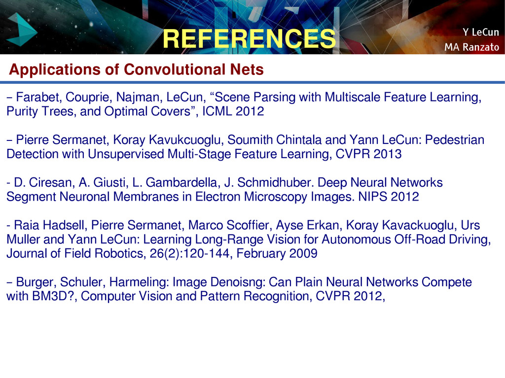
202. Y LeCun MA Ranzato REFERENCES Applications of Convolutional Nets – Farabet, Couprie, Najman, LeCun, “Scene Parsing with Multiscale Feature Learning, Purity Trees, and Optimal Covers”, ICML 2012 – Pierre Sermanet, Koray Kavukcuoglu, Soumith Chintala and Yann LeCun: Pedestrian Detection with Unsupervised Multi-Stage Feature Learning, CVPR 2013 - D. Ciresan, A. Giusti, L. Gambardella, J. Schmidhuber. Deep Neural Networks Segment Neuronal Membranes in Electron Microscopy Images. NIPS 2012 - Raia Hadsell, Pierre Sermanet, Marco Scoffier, Ayse Erkan, Koray Kavackuoglu, Urs Muller and Yann LeCun: Learning Long-Range Vision for Autonomous Off-Road Driving, Journal of Field Robotics, 26(2):120-144, February 2009 – Burger, Schuler, Harmeling: Image Denoisng: Can Plain Neural Networks Compete with BM3D?, Computer Vision and Pattern Recognition, CVPR 2012,
203. Y LeCun MA Ranzato REFERENCES Applications of RNNs – Mikolov “Statistical language models based on neural networks” PhD thesis 2012 – Boden “A guide to RNNs and backpropagation” Tech Report 2002 – Hochreiter, Schmidhuber “Long short term memory” Neural Computation 1997 – Graves “Offline arabic handwrting recognition with multidimensional neural networks” Springer 2012 – Graves “Speech recognition with deep recurrent neural networks” ICASSP 2013
204. Y LeCun MA Ranzato REFERENCES Deep Learning & Energy-Based Models – Y. Bengio, Learning Deep Architectures for AI, Foundations and Trends in Machine Learning, 2(1), pp.1-127, 2009. – LeCun, Chopra, Hadsell, Ranzato, Huang: A Tutorial on Energy-Based Learning, in Bakir, G. and Hofman, T. and Schölkopf, B. and Smola, A. and Taskar, B. (Eds), Predicting Structured Data, MIT Press, 2006 – M. Ranzato Ph.D. Thesis “Unsupervised Learning of Feature Hierarchies” NYU 2009 Practical guide – Y. LeCun et al. Efficient BackProp, Neural Networks: Tricks of the Trade, 1998 – L. Bottou, Stochastic gradient descent tricks, Neural Networks, Tricks of the Trade Reloaded, LNCS 2012. – Y. Bengio, Practical recommendations for gradient-based training of deep architectures, ArXiv 2012