Yoshua Bengio AAAI 2013: Deep Learning of Representations

http://www.iro.umontreal.ca/~bengioy/talks/aaai2013-tutorial.pdf

Transcript

1. Deep  Learning  of   Representa0ons     AAAI  Tutorial       Yoshua  Bengio     July  14th  2013,  Bellevue,  WA,  USA      
2. Outline of the Tutorial 1.  Mo8va8ons  and  Scope   2.  Algorithms   3.  Prac8cal  Considera8ons   4.  Challenges   See  (Bengio,  Courville  &  Vincent  2013)     “Unsupervised  Feature  Learning  and  Deep  Learning:  A  Review  and  New  Perspec8ves”   and  http://www.iro.umontreal.ca/~bengioy/talks/deep-learning-tutorial-aaai2013.html  for  a   pdf  of  the  slides  and  a  detailed  list  of  references.  
3. Ultimate Goals •  AI   •  Needs  knowledge   •  Needs  learning                                   (involves  priors  +  op#miza#on/search)   •  Needs  generaliza0on                               (guessing  where  probability  mass  concentrates)   •  Needs  ways  to  fight  the  curse  of  dimensionality   (exponen8ally  many  configura8ons  of  the  variables  to  consider)   •  Needs  disentangling  the  underlying  explanatory  factors   (making  sense  of  the  data)   3  
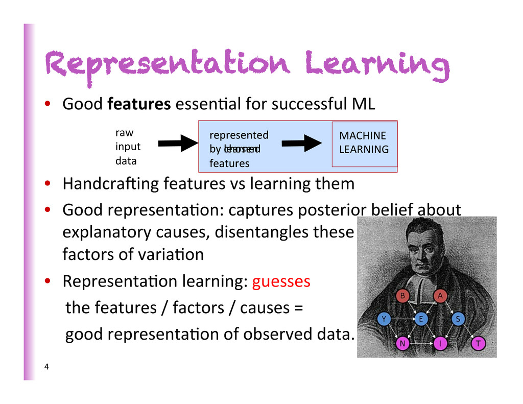
4. •  Good  features  essen8al  for  successful  ML   •  HandcraZing  features  vs  learning  them   •  Good  representa8on:  captures  posterior  belief  about   explanatory  causes,  disentangles  these  underlying   factors  of  varia8on   •  Representa8on  learning:  guesses            the  features  /  factors  /  causes  =              good  representa8on  of  observed  data.   Representation Learning 4   raw   input   data   represented   by  chosen   features   MACHINE   LEARNING     represented   by  learned   features  
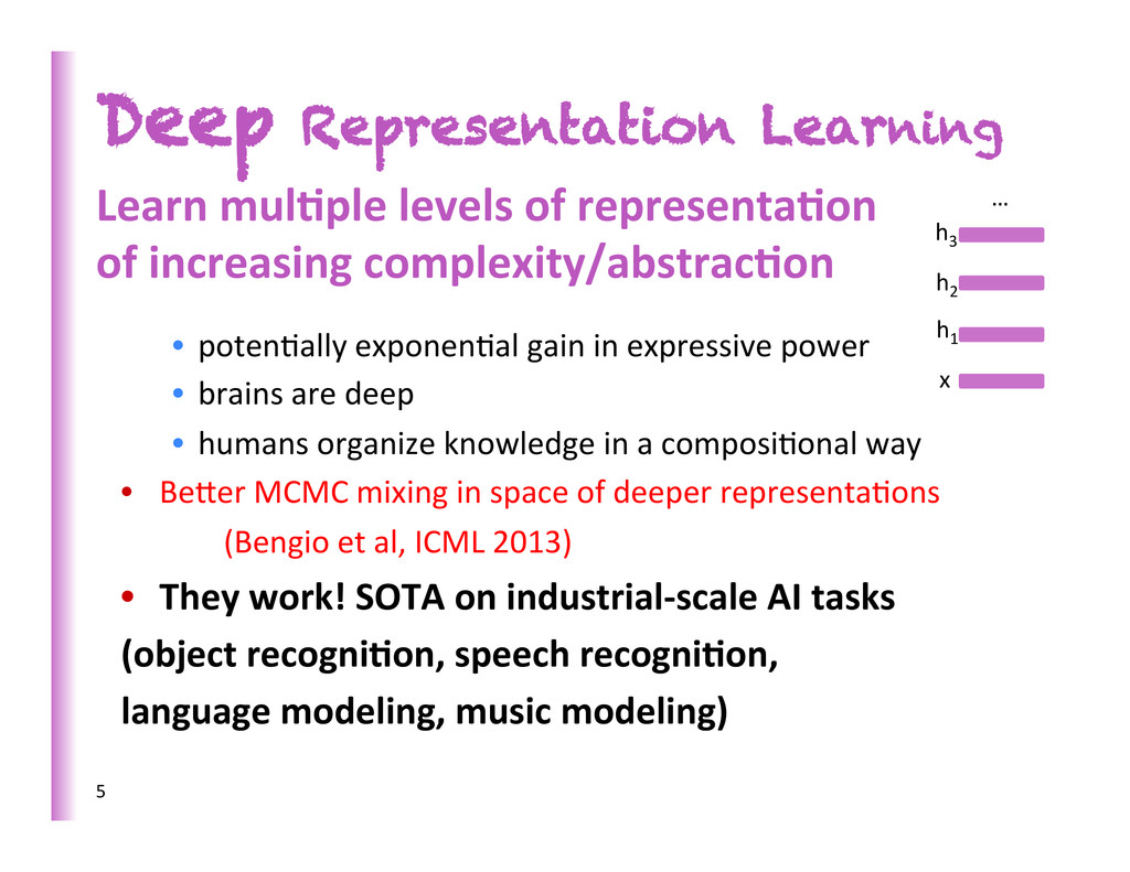
5. Deep Representation Learning Learn  mul0ple  levels  of  representa0on   of  increasing  complexity/abstrac0on         5   x   h3   h2   h1   …   •  poten8ally  exponen8al  gain  in  expressive  power   •  brains  are  deep   •  humans  organize  knowledge  in  a  composi8onal  way   •  Beber  MCMC  mixing  in  space  of  deeper  representa8ons    (Bengio  et  al,  ICML  2013)   •  They  work!  SOTA  on  industrial-­‐scale  AI  tasks   (object  recogni0on,  speech  recogni0on,     language  modeling,  music  modeling)    
6. Deep Learning   When  the  number  of  levels  can  be  data-­‐ selected,  this  is  a  deep  architecture       6   x   h3   h2   h1   …  
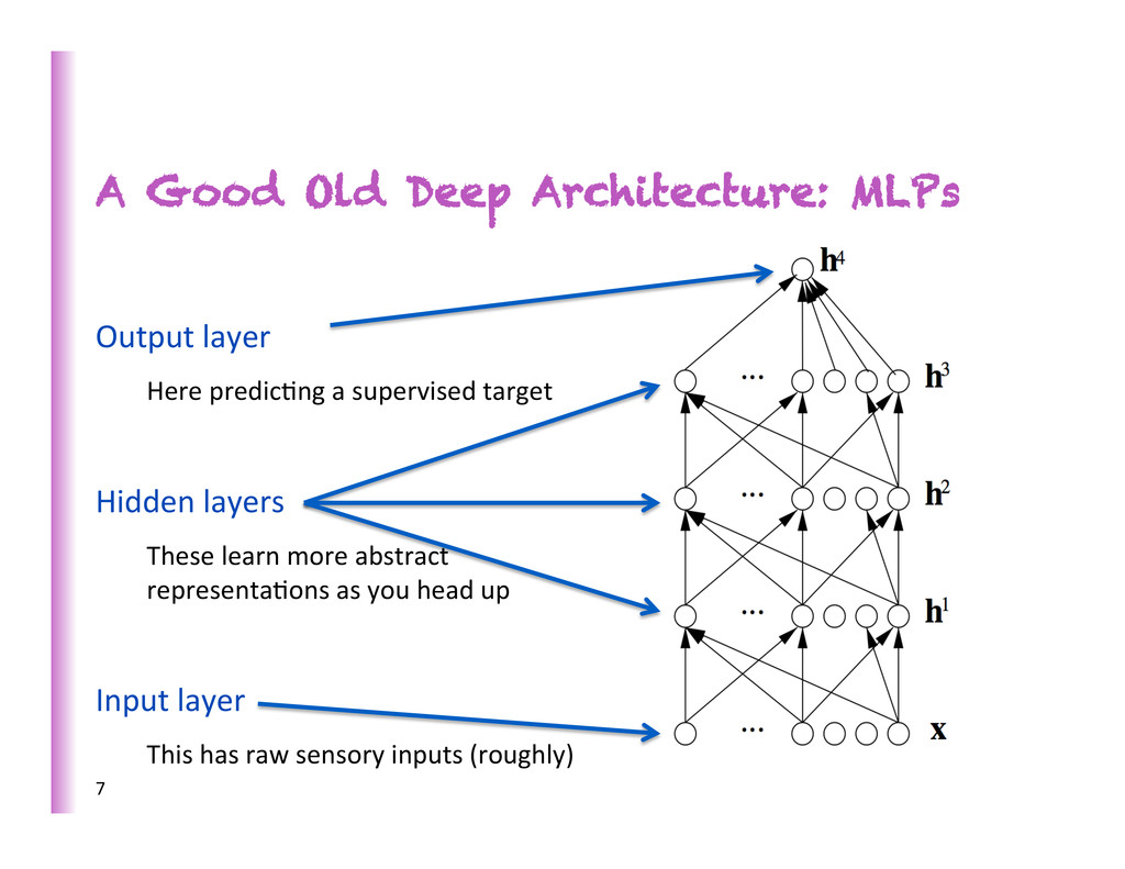
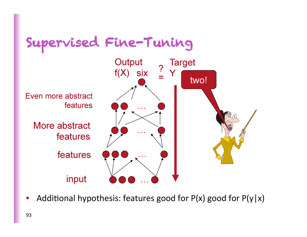
7. A Good Old Deep Architecture: MLPs   Output  layer   Here  predic8ng  a  supervised  target     Hidden  layers   These  learn  more  abstract   representa8ons  as  you  head  up     Input  layer   This  has  raw  sensory  inputs  (roughly)   7  
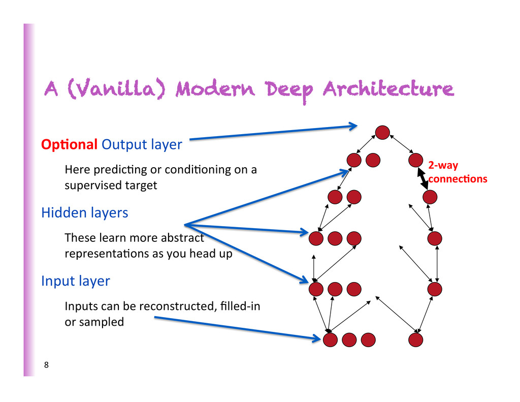
8. A (Vanilla) Modern Deep Architecture   Op0onal  Output  layer   Here  predic8ng  or  condi8oning  on  a   supervised  target   Hidden  layers   These  learn  more  abstract   representa8ons  as  you  head  up   Input  layer   Inputs  can  be  reconstructed,  filled-­‐in   or  sampled     8   2-­‐way   connec0ons  
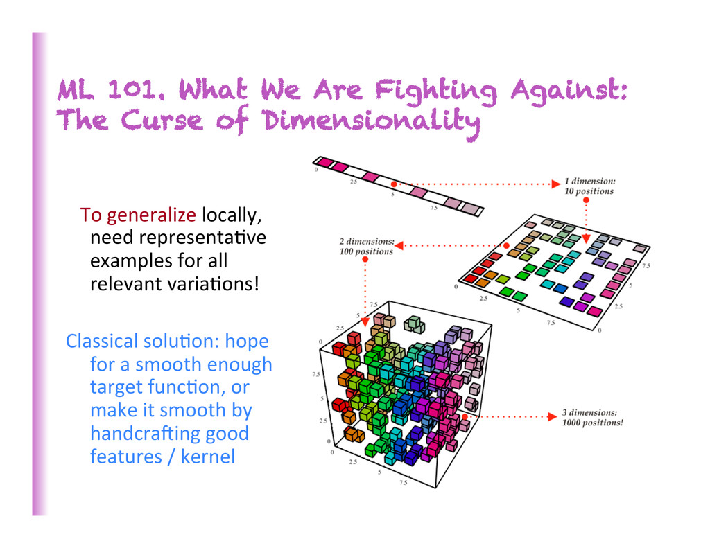
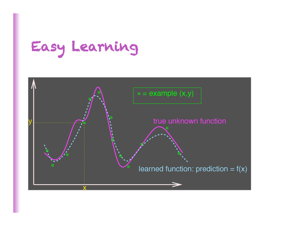
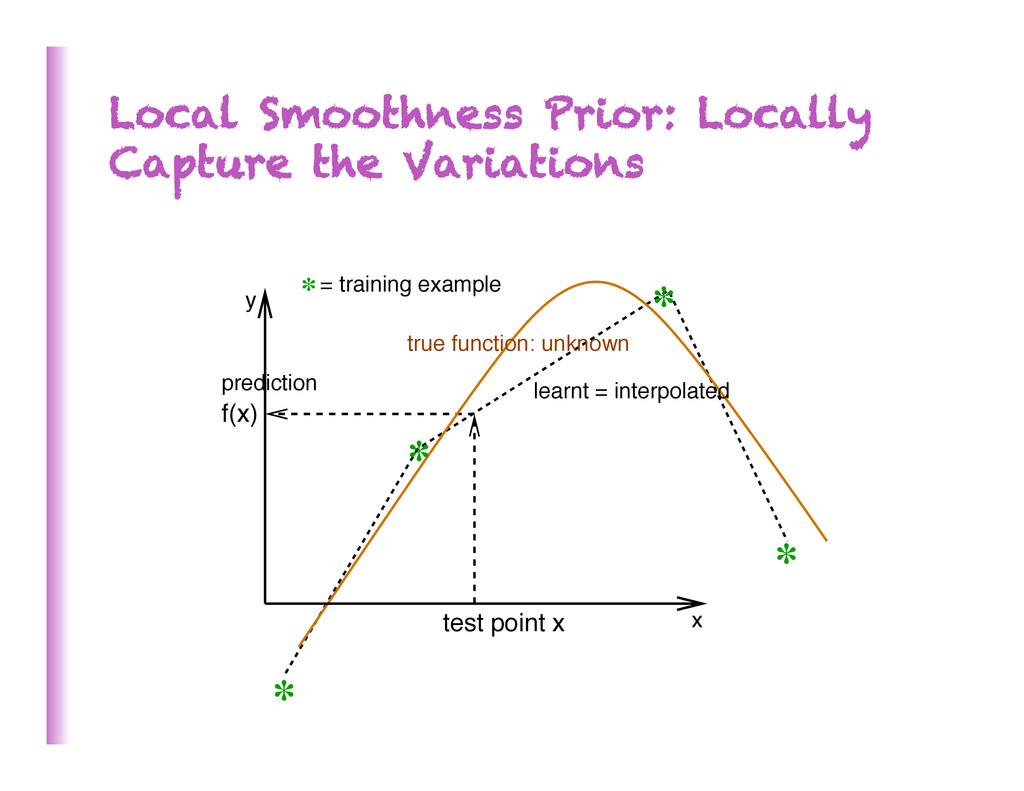
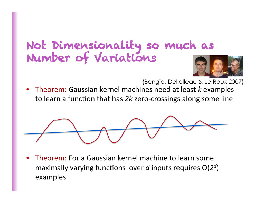
9. ML 101. What We Are Fighting Against: The Curse of Dimensionality      To  generalize  locally,   need  representa8ve   examples  for  all   relevant  varia8ons!     Classical  solu8on:  hope   for  a  smooth  enough   target  func8on,  or   make  it  smooth  by   handcraZing  good   features  /  kernel  
10. Easy Learning learned function: prediction = f(x) * * * * * * * * * * * * * true unknown function = example (x,y) * x y
11. Local Smoothness Prior: Locally Capture the Variations * y x * learnt = interpolated f(x) prediction true function: unknown * * test point x * = training example
12. However, Real Data Are near Highly Curved Sub-Manifolds 12  
13. Not Dimensionality so much as Number of Variations •  Theorem:  Gaussian  kernel  machines  need  at  least  k  examples   to  learn  a  func8on  that  has  2k  zero-­‐crossings  along  some  line             •  Theorem:  For  a  Gaussian  kernel  machine  to  learn  some   maximally  varying  func8ons    over  d  inputs  requires  O(2d)   examples     (Bengio, Dellalleau & Le Roux 2007)
14. Putting Probability Mass where Structure is Plausible •  Empirical  distribu8on:  mass  at   training  examples   14   •  Smoothness:  spread  mass  around   •  Insufficient   •  Guess  some  ‘structure’  and   generalize  accordingly  
15. Is there any hope to generalize non-locally? Yes! Need good priors! 15  
16. Six Good Reasons to Explore Representation Learning Part  1   16  
17. #1 Learning features, not just handcrafting them Most  ML  systems  use  very  carefully  hand-­‐designed   features  and  representa8ons   Many  prac88oners  are  very  experienced  –  and  good  –  at  such   feature  design  (or  kernel  design)   “Machine  learning”  oZen  reduces  to  linear  models  (including   CRFs)  and  nearest-­‐neighbor-­‐like  features/models  (including  n-­‐ grams,  kernel  SVMs,  etc.)     Hand-­‐craNing  features  is  0me-­‐consuming,  briOle,  incomplete   17  
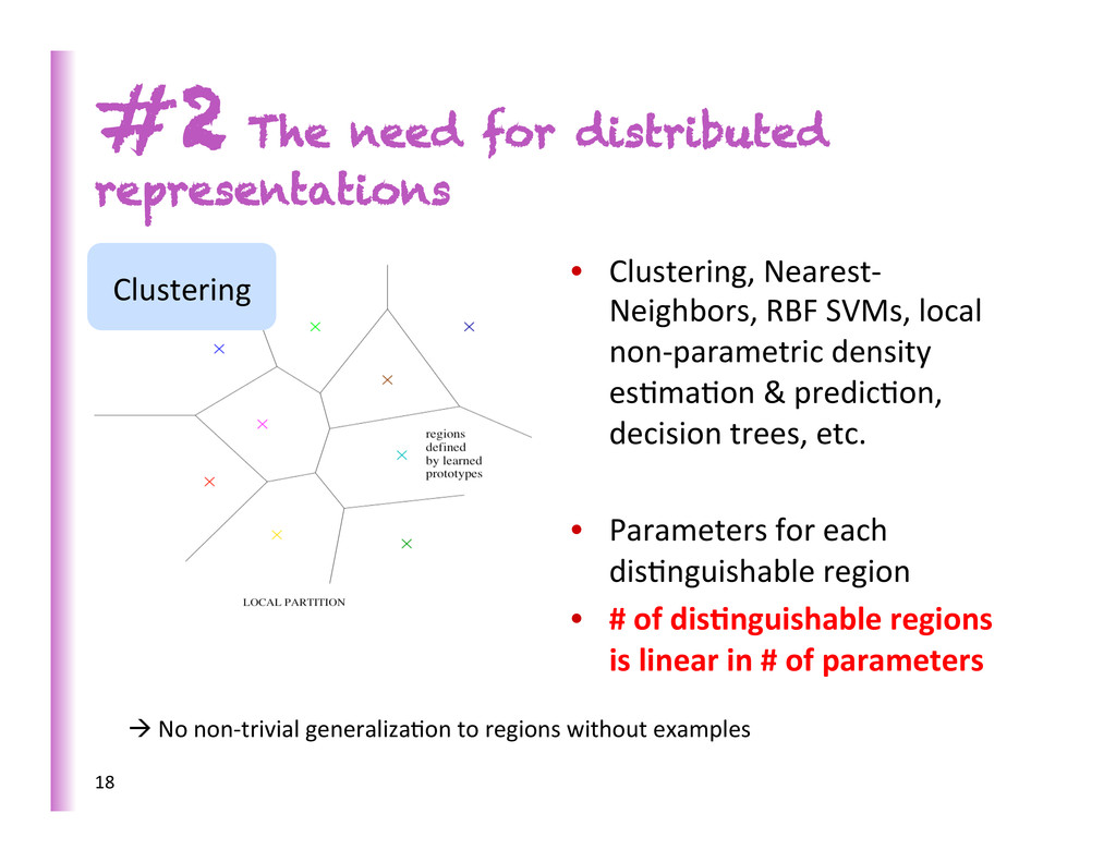
18. •  Clustering,  Nearest-­‐ Neighbors,  RBF  SVMs,  local   non-­‐parametric  density   es8ma8on  &  predic8on,   decision  trees,  etc.   •  Parameters  for  each   dis8nguishable  region   •  #  of  dis0nguishable  regions   is  linear  in  #  of  parameters   #2 The need for distributed representations Clustering   18   à  No  non-­‐trivial  generaliza8on  to  regions  without  examples  
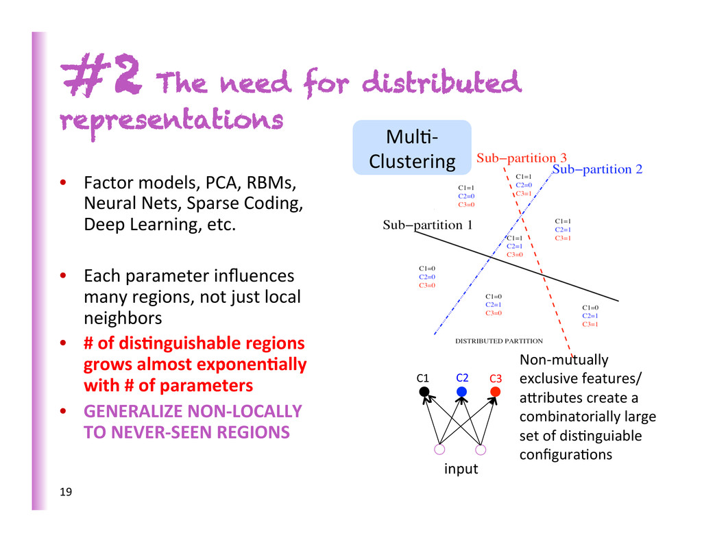
19. •  Factor  models,  PCA,  RBMs,   Neural  Nets,  Sparse  Coding,   Deep  Learning,  etc.   •  Each  parameter  influences   many  regions,  not  just  local   neighbors   •  #  of  dis0nguishable  regions   grows  almost  exponen0ally   with  #  of  parameters   •  GENERALIZE  NON-­‐LOCALLY   TO  NEVER-­‐SEEN  REGIONS   #2 The need for distributed representations Mul8-­‐   Clustering   19   C1   C2   C3   input   Non-­‐mutually   exclusive  features/ abributes  create  a   combinatorially  large   set  of  dis8nguiable   configura8ons  
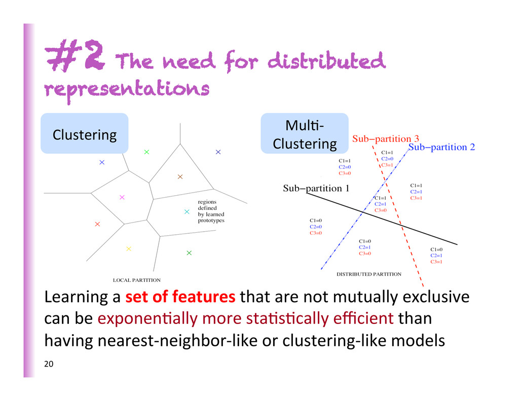
20. #2 The need for distributed representations Mul8-­‐   Clustering   Clustering   20   Learning  a  set  of  features  that  are  not  mutually  exclusive   can  be  exponen8ally  more  sta8s8cally  efficient  than   having  nearest-­‐neighbor-­‐like  or  clustering-­‐like  models  
21. #3 Unsupervised feature learning Today,  most  prac8cal  ML  applica8ons  require  (lots  of)   labeled  training  data   But  almost  all  data  is  unlabeled   The  brain  needs  to  learn  about  1014  synap8c  strengths   …  in  about  109  seconds   Labels  cannot  possibly  provide  enough  informa8on   Most  informa8on  acquired  in  an  unsupervised  fashion   21  
22. #3 How do humans generalize from very few examples? 22   •  They  transfer  knowledge  from  previous  learning:   •  Representa8ons   •  Explanatory  factors   •  Previous  learning  from:  unlabeled  data                    +  labels  for  other  tasks   •  Prior:  shared  underlying  explanatory  factors,  in   par0cular  between  P(x)  and  P(Y|x)      
23. #3 Sharing Statistical Strength by Semi-Supervised Learning •  Hypothesis:  P(x)  shares  structure  with  P(y|x)   purely   supervised   semi-­‐   supervised   23  
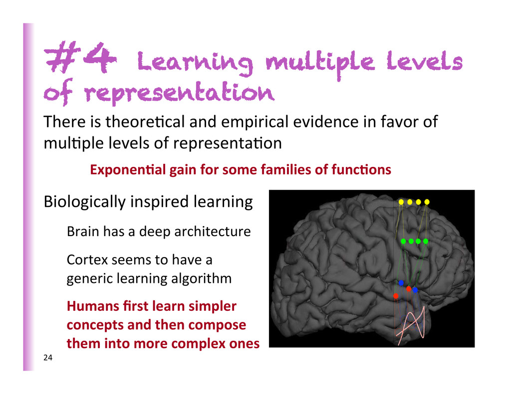
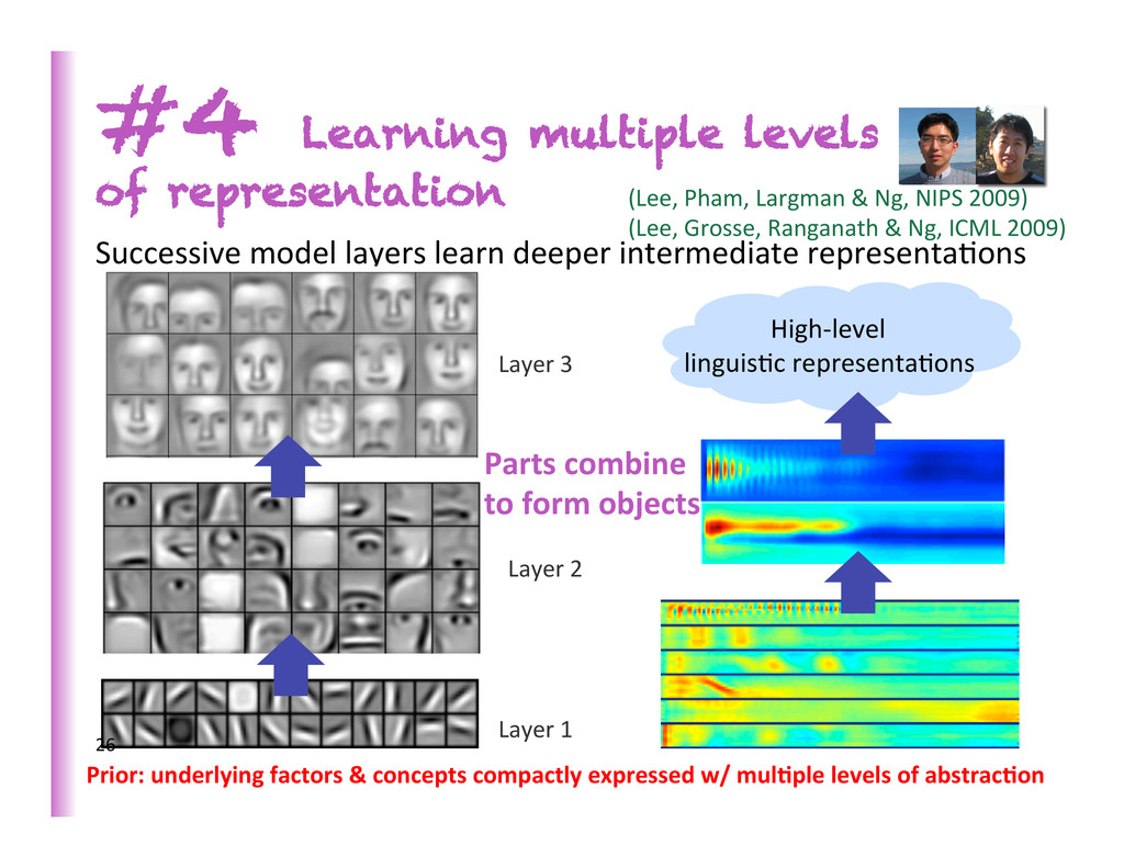
24. #4 Learning multiple levels of representation There  is  theore8cal  and  empirical  evidence  in  favor  of   mul8ple  levels  of  representa8on    Exponen0al  gain  for  some  families  of  func0ons   Biologically  inspired  learning   Brain  has  a  deep  architecture   Cortex  seems  to  have  a     generic  learning  algorithm     Humans  first  learn  simpler     concepts  and  then  compose     them  into  more  complex  ones     24  
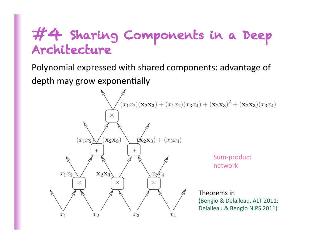
25. #4 Sharing Components in a Deep Architecture Sum-­‐product   network   Polynomial  expressed  with  shared  components:  advantage  of   depth  may  grow  exponen8ally       Theorems  in     (Bengio  &  Delalleau,  ALT  2011;   Delalleau  &  Bengio  NIPS  2011)  
26. #4 Learning multiple levels of representation Successive  model  layers  learn  deeper  intermediate  representa8ons     Layer  1   Layer  2   Layer  3   High-­‐level   linguis8c  representa8ons   (Lee,  Pham,  Largman  &  Ng,  NIPS  2009)   (Lee,  Grosse,  Ranganath  &  Ng,  ICML  2009)     26   Prior:  underlying  factors  &  concepts  compactly  expressed  w/  mul0ple  levels  of  abstrac0on     Parts  combine   to  form  objects  
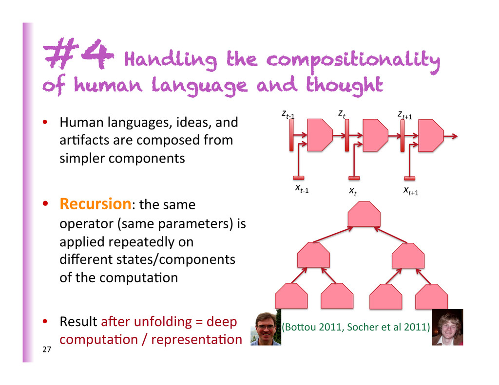
27. #4 Handling the compositionality of human language and thought •  Human  languages,  ideas,  and   ar8facts  are  composed  from   simpler  components   •  Recursion:  the  same   operator  (same  parameters)  is   applied  repeatedly  on   different  states/components   of  the  computa8on   •  Result  aZer  unfolding  =  deep   computa8on  /  representa8on   xt-­‐1   xt   xt+1   zt-­‐1   zt   zt+1   27   (Bobou  2011,  Socher  et  al  2011)  
28. #5 Multi-Task Learning •  Generalizing  beber  to  new  tasks   (tens  of  thousands!)  is  crucial  to   approach  AI   •  Deep  architectures  learn  good   intermediate  representa8ons  that   can  be  shared  across  tasks            (Collobert  &  Weston  ICML  2008,            Bengio  et  al  AISTATS  2011)   •  Good  representa8ons  that   disentangle  underlying  factors  of   varia8on  make  sense  for  many  tasks   because  each  task  concerns  a   subset  of  the  factors   28   raw input x task 1 output y1 task 3 output y3 task 2 output y2 Task  A   Task  B   Task  C   Prior:  shared  underlying  explanatory  factors  between  tasks       E.g.  dic8onary,  with  intermediate   concepts  re-­‐used  across  many  defini8ons  
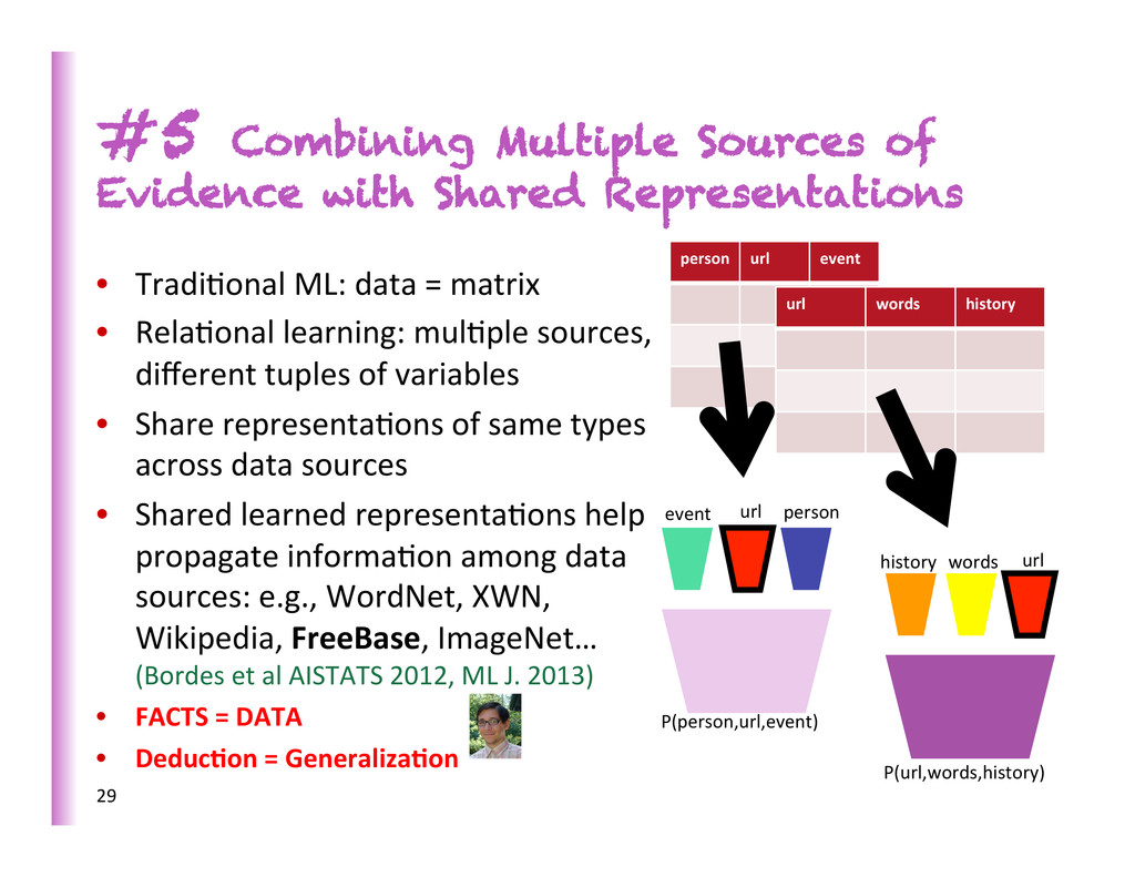
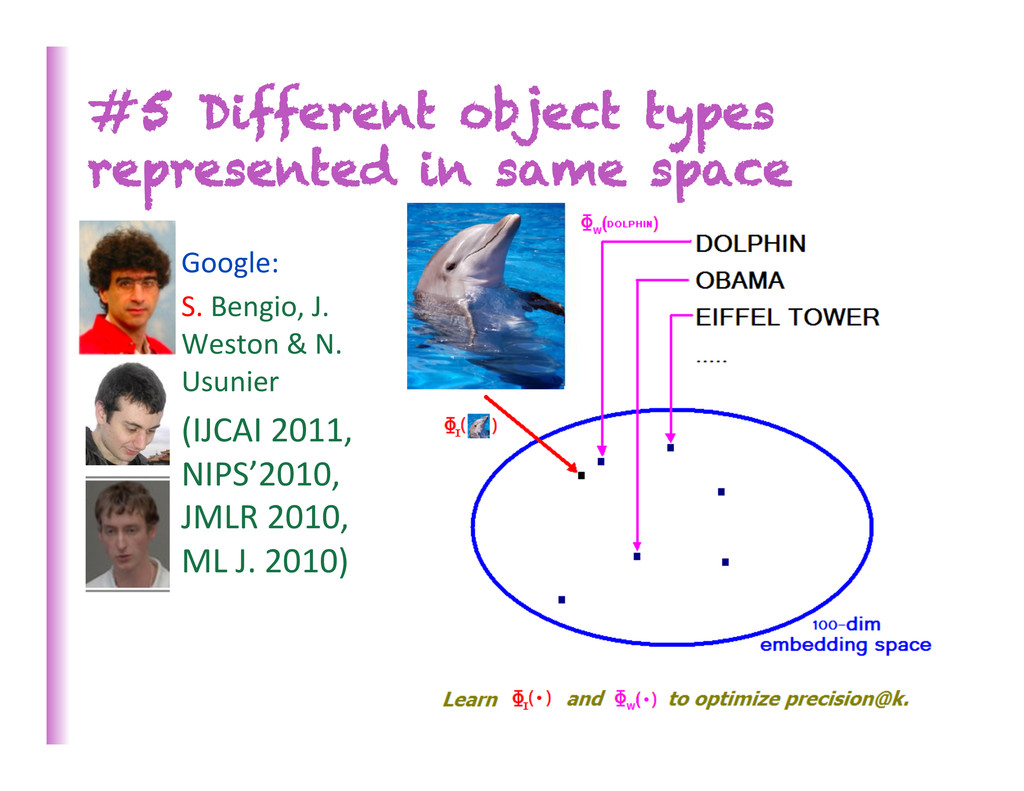
29. #5 Combining Multiple Sources of Evidence with Shared Representations •  Tradi8onal  ML:  data  =  matrix   •  Rela8onal  learning:  mul8ple  sources,   different  tuples  of  variables   •  Share  representa8ons  of  same  types   across  data  sources   •  Shared  learned  representa8ons  help   propagate  informa8on  among  data   sources:  e.g.,  WordNet,  XWN,   Wikipedia,  FreeBase,  ImageNet… (Bordes  et  al  AISTATS  2012,  ML  J.  2013)   •  FACTS  =  DATA   •  Deduc0on  =  Generaliza0on   29   person   url   event   url   words   history   person   url   event   P(person,url,event)   url   words   history   P(url,words,history)  
30. #5 Different object types represented in same space Google:   S.  Bengio,  J.   Weston  &  N.   Usunier   (IJCAI  2011,   NIPS’2010,   JMLR  2010,   ML  J.  2010)  
31. #6 Invariance and Disentangling •  Invariant  features   •  Which  invariances?   •  Alterna8ve:  learning  to  disentangle  factors   •  Good  disentangling  à      avoid  the  curse  of  dimensionality   31  
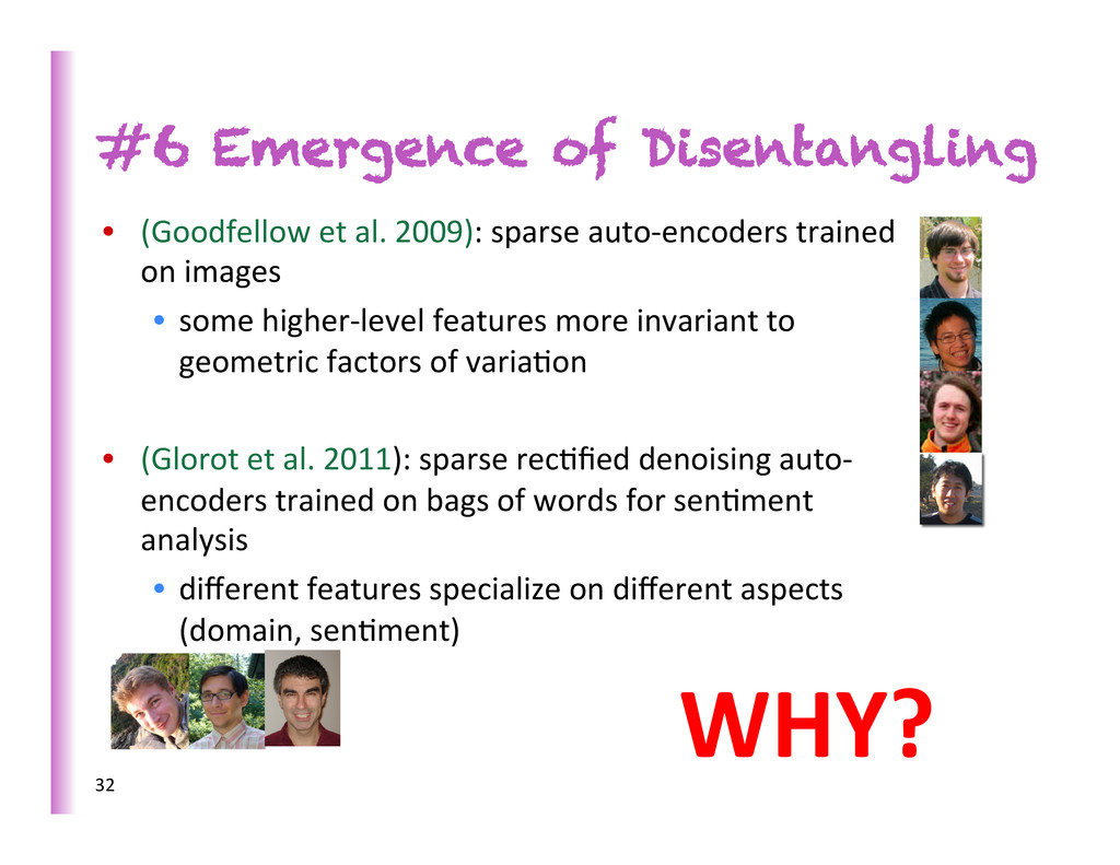
32. #6 Emergence of Disentangling •  (Goodfellow  et  al.  2009):  sparse  auto-­‐encoders  trained   on  images     •  some  higher-­‐level  features  more  invariant  to   geometric  factors  of  varia8on     •  (Glorot  et  al.  2011):  sparse  rec8fied  denoising  auto-­‐ encoders  trained  on  bags  of  words  for  sen8ment   analysis   •  different  features  specialize  on  different  aspects   (domain,  sen8ment)   32   WHY?  
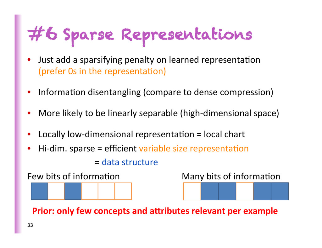
33. #6 Sparse Representations •  Just  add  a  sparsifying  penalty  on  learned  representa8on         (prefer  0s  in  the  representa8on)   •  Informa8on  disentangling  (compare  to  dense  compression)   •  More  likely  to  be  linearly  separable  (high-­‐dimensional  space)   •  Locally  low-­‐dimensional  representa8on  =  local  chart   •  Hi-­‐dim.  sparse  =  efficient  variable  size  representa8on                  =  data  structure   Few  bits  of  informa8on                                                        Many  bits  of  informa8on   33   Prior:  only  few  concepts  and  aOributes  relevant  per  example    
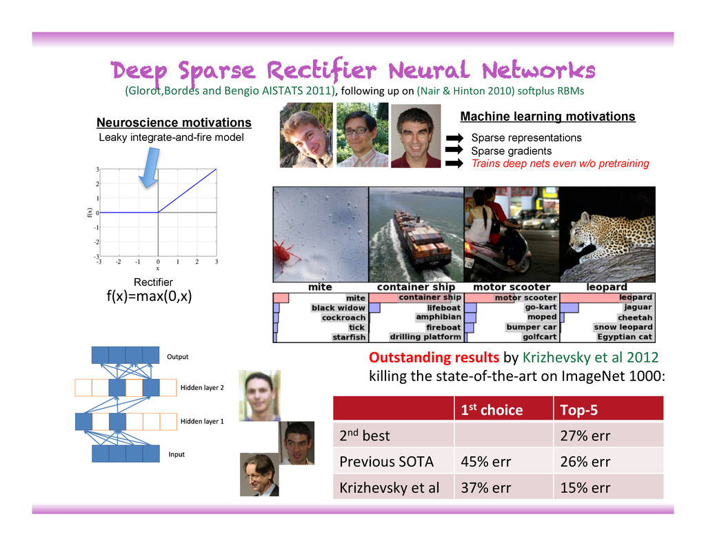
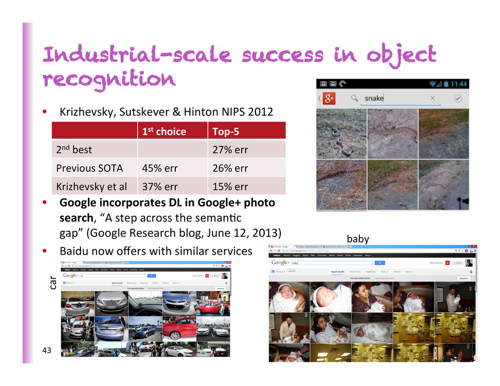
34. Sparse gradients Trains deep nets even w/o pretraining Deep Sparse Rectifier Neural Networks  (Glorot,Bordes  and  Bengio  AISTATS  2011),  following  up  on  (Nair  &  Hinton  2010)  soZplus  RBMs   Leaky integrate-and-fire model Rectifier Neuroscience motivations Machine learning motivations Sparse representations f(x)=max(0,x)   Outstanding  results  by  Krizhevsky  et  al  2012   killing  the  state-­‐of-­‐the-­‐art  on  ImageNet  1000:       1st  choice   Top-­‐5   2nd  best   27%  err   Previous  SOTA   45%  err   26%  err   Krizhevsky  et  al   37%  err   15%  err  
35. Temporal Coherence and Scales •  Hints  from  nature  about  different  explanatory  factors:   •  Rapidly  changing  factors  (oZen  noise)   •  Slowly  changing  (generally  more  abstract)   •  Different  factors  at  different  8me  scales   •  Exploit  those  hints  to  disentangle  beber!   •  (Becker  &  Hinton  1993,  Wiskob  &  Sejnowski  2002,  Hurri  &   Hyvarinen  2003,  Berkes  &  Wiskob  2005,  Mobahi  et  al   2009,  Bergstra  &  Bengio  2009)  
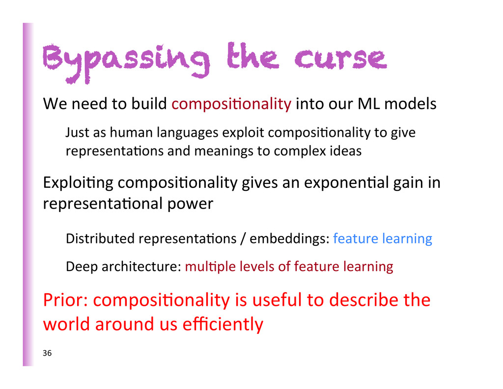
36. Bypassing the curse We  need  to  build  composi8onality  into  our  ML  models     Just  as  human  languages  exploit  composi8onality  to  give   representa8ons  and  meanings  to  complex  ideas   Exploi8ng  composi8onality  gives  an  exponen8al  gain  in   representa8onal  power   Distributed  representa8ons  /  embeddings:  feature  learning   Deep  architecture:  mul8ple  levels  of  feature  learning   Prior:  composi8onality  is  useful  to  describe  the   world  around  us  efficiently     36  
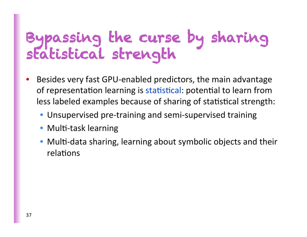
37. Bypassing the curse by sharing statistical strength •  Besides  very  fast  GPU-­‐enabled  predictors,  the  main  advantage   of  representa8on  learning  is  sta8s8cal:  poten8al  to  learn  from   less  labeled  examples  because  of  sharing  of  sta8s8cal  strength:   •  Unsupervised  pre-­‐training  and  semi-­‐supervised  training   •  Mul8-­‐task  learning   •  Mul8-­‐data  sharing,  learning  about  symbolic  objects  and  their   rela8ons   37  
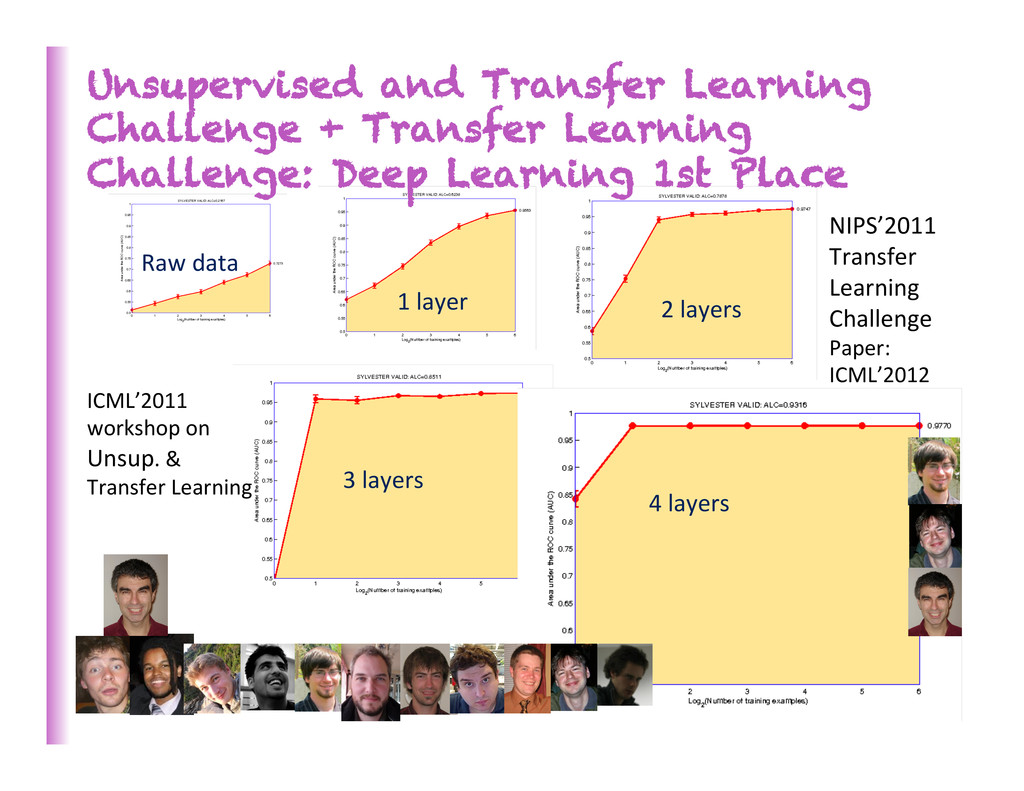
38. Raw  data   1  layer   2  layers   4  layers   3  layers   ICML’2011   workshop  on   Unsup.  &   Transfer  Learning   NIPS’2011   Transfer   Learning   Challenge     Paper:   ICML’2012   Unsupervised and Transfer Learning Challenge + Transfer Learning Challenge: Deep Learning 1st Place
39. Why now? Despite  prior  inves8ga8on  and  understanding  of  many  of  the   algorithmic  techniques  …   Before  2006  training  deep  architectures  was  unsuccessful   (except  for  convolu8onal  neural  nets  when  used  by  people  who  speak  French)   What  has  changed?   •  New  methods  for  unsupervised  pre-­‐training  have  been   developed  (variants  of  Restricted  Boltzmann  Machines  =   RBMs,  regularized  auto-­‐encoders,  sparse  coding,  etc.)   •  New  methods  to  successfully  train  deep  supervised  nets   even  without  unsupervised  pre-­‐training   •  Successful  real-­‐world  applica8ons,  winning  challenges  and   bea8ng  SOTAs  in  various  areas,  large-­‐scale  industrial  apps   39  
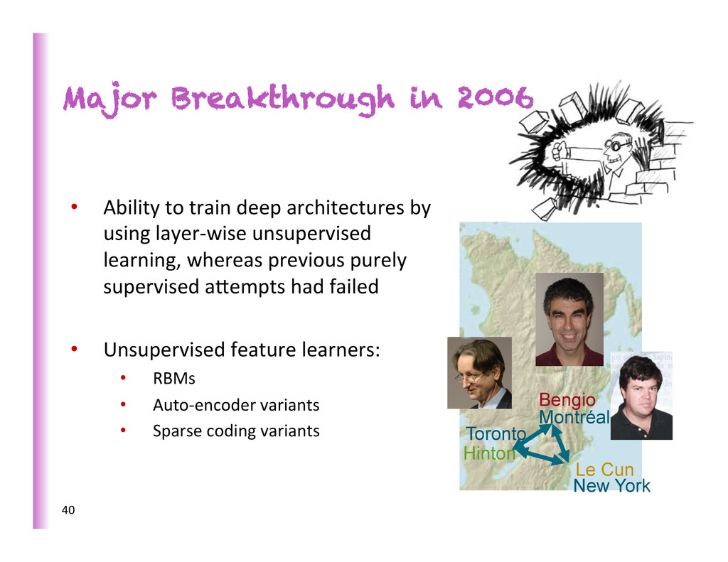
40. Montréal Toronto Bengio Hinton Le Cun Major Breakthrough in 2006 •  Ability  to  train  deep  architectures  by   using  layer-­‐wise  unsupervised   learning,  whereas  previous  purely   supervised  abempts  had  failed   •  Unsupervised  feature  learners:   •  RBMs   •  Auto-­‐encoder  variants   •  Sparse  coding  variants   New York 40  
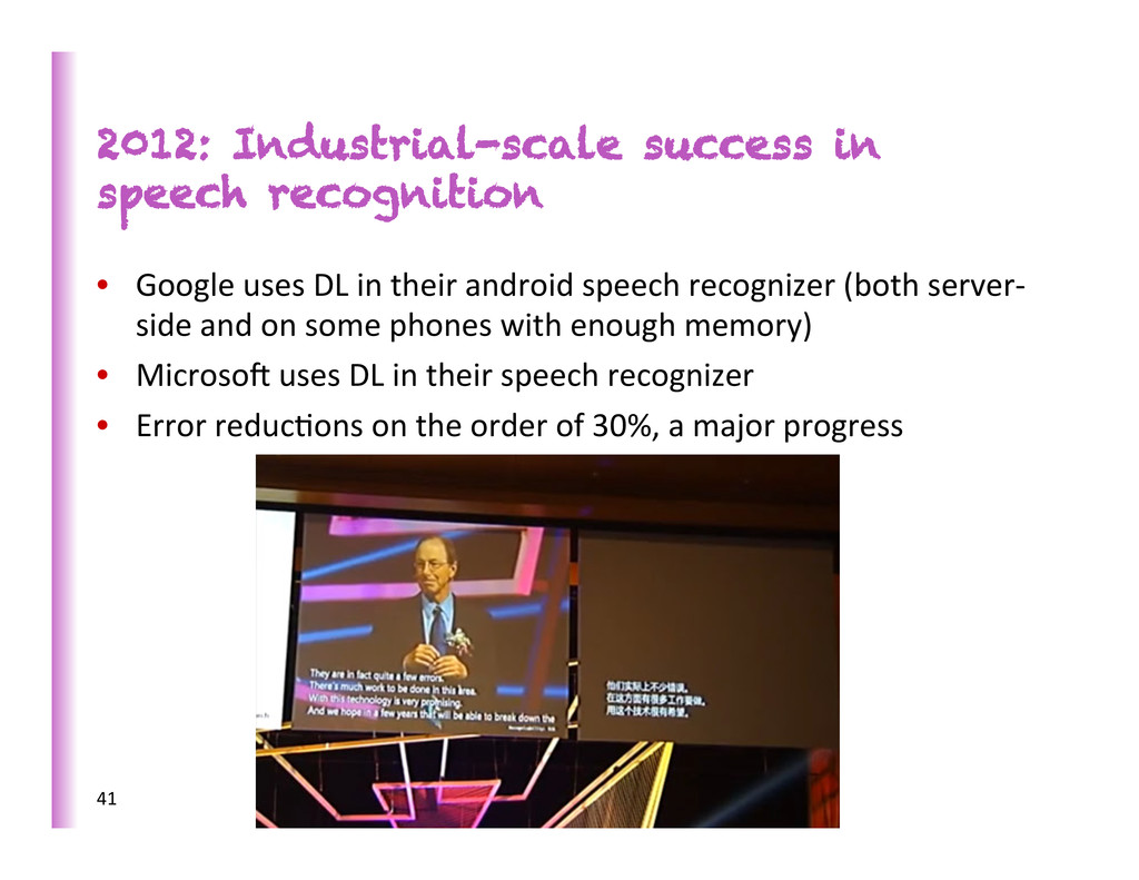
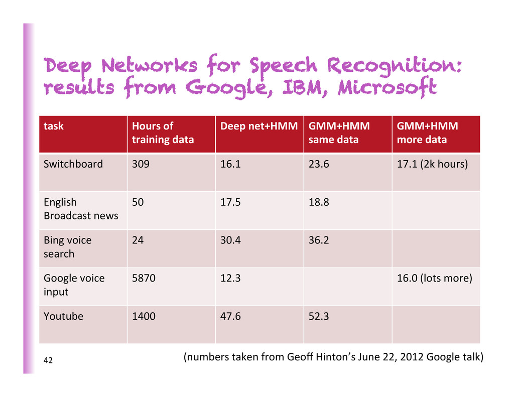
41. 2012: Industrial-scale success in speech recognition •  Google  uses  DL  in  their  android  speech  recognizer  (both  server-­‐ side  and  on  some  phones  with  enough  memory)   •  MicrosoZ  uses  DL  in  their  speech  recognizer   •  Error  reduc8ons  on  the  order  of  30%,  a  major  progress   41  
42. Deep Networks for Speech Recognition: results from Google, IBM, Microsoft task   Hours  of   training  data   Deep  net+HMM   GMM+HMM   same  data   GMM+HMM   more  data   Switchboard   309   16.1   23.6   17.1  (2k  hours)   English   Broadcast  news   50   17.5   18.8   Bing  voice   search   24   30.4   36.2   Google  voice   input   5870   12.3   16.0  (lots  more)   Youtube   1400   47.6   52.3   42   (numbers  taken  from  Geoff  Hinton’s  June  22,  2012  Google  talk)    
43. Industrial-scale success in object recognition •  Krizhevsky,  Sutskever  &  Hinton  NIPS  2012     •  Google  incorporates  DL  in  Google+  photo   search,  “A  step  across  the  seman8c   gap”  (Google  Research  blog,  June  12,  2013)   •  Baidu  now  offers  with  similar  services       43   1st  choice   Top-­‐5   2nd  best   27%  err   Previous  SOTA   45%  err   26%  err   Krizhevsky  et  al   37%  err   15%  err   baby   car  
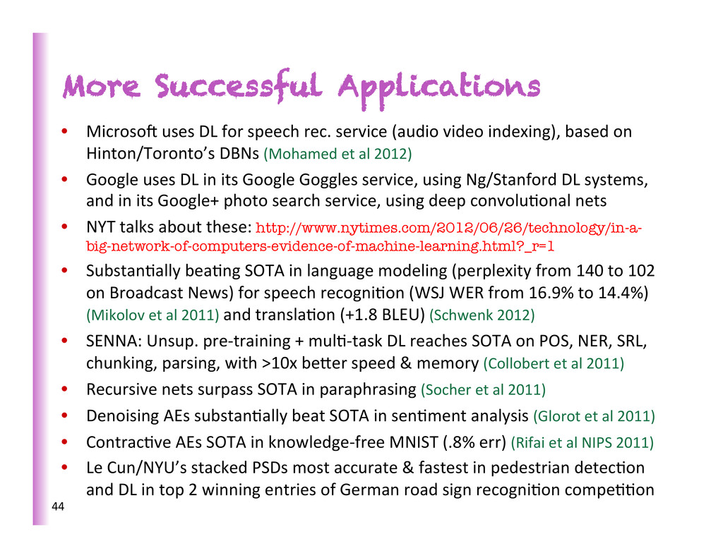
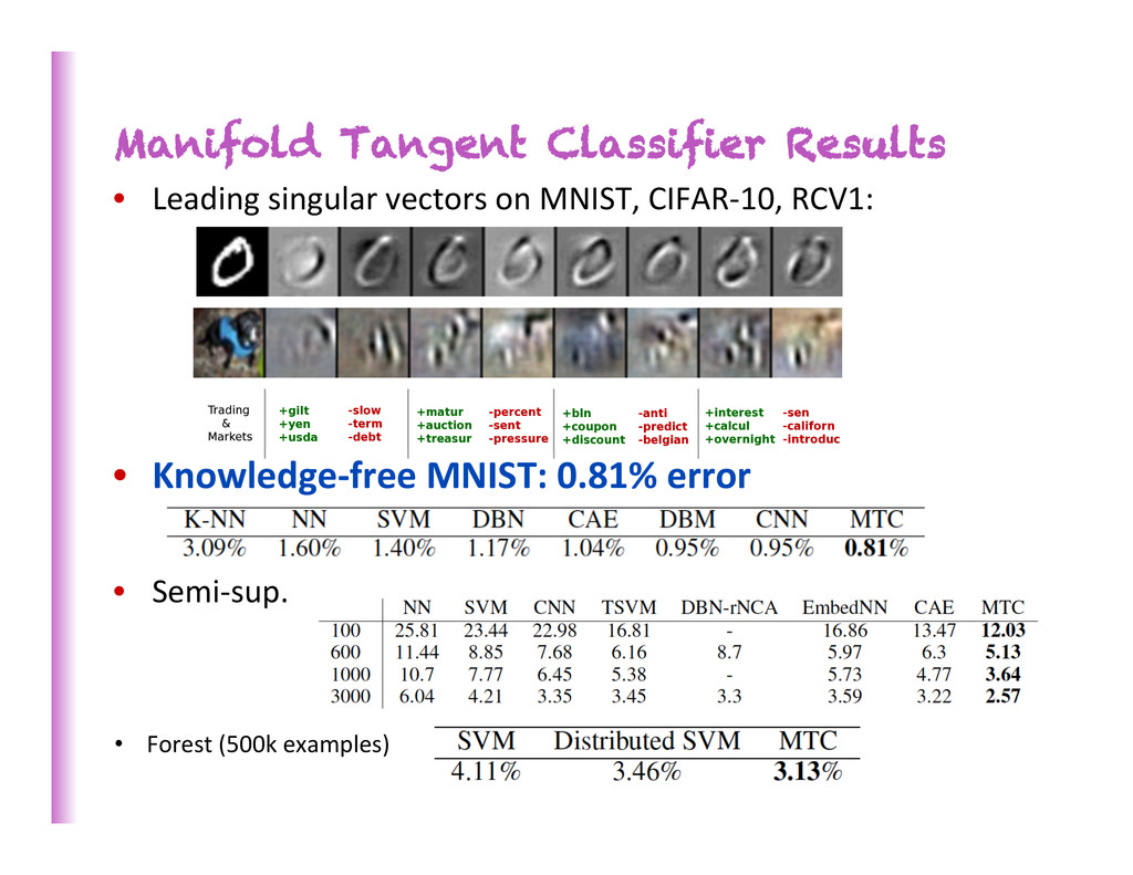
44. More Successful Applications •  MicrosoZ  uses  DL  for  speech  rec.  service  (audio  video  indexing),  based  on   Hinton/Toronto’s  DBNs  (Mohamed  et  al  2012)   •  Google  uses  DL  in  its  Google  Goggles  service,  using  Ng/Stanford  DL  systems,   and  in  its  Google+  photo  search  service,  using  deep  convolu8onal  nets   •  NYT  talks  about  these:  http://www.nytimes.com/2012/06/26/technology/in-a- big-network-of-computers-evidence-of-machine-learning.html?_r=1 •  Substan8ally  bea8ng  SOTA  in  language  modeling  (perplexity  from  140  to  102   on  Broadcast  News)  for  speech  recogni8on  (WSJ  WER  from  16.9%  to  14.4%)   (Mikolov  et  al  2011)  and  transla8on  (+1.8  BLEU)  (Schwenk  2012)   •  SENNA:  Unsup.  pre-­‐training  +  mul8-­‐task  DL  reaches  SOTA  on  POS,  NER,  SRL,   chunking,  parsing,  with  >10x  beber  speed  &  memory  (Collobert  et  al  2011)   •  Recursive  nets  surpass  SOTA  in  paraphrasing  (Socher  et  al  2011)   •  Denoising  AEs  substan8ally  beat  SOTA  in  sen8ment  analysis  (Glorot  et  al  2011)   •  Contrac8ve  AEs  SOTA  in  knowledge-­‐free  MNIST  (.8%  err)  (Rifai  et  al  NIPS  2011)   •  Le  Cun/NYU’s  stacked  PSDs  most  accurate  &  fastest  in  pedestrian  detec8on   and  DL  in  top  2  winning  entries  of  German  road  sign  recogni8on  compe88on     44  
45. Already Many NLP Applications of DL •  Language  Modeling  (Speech  Recogni8on,  Machine  Transla8on)   •  Acous8c  Modeling   •  Part-­‐Of-­‐Speech  Tagging   •  Chunking   •  Named  En8ty  Recogni8on   •  Seman8c  Role  Labeling   •  Parsing   •  Sen8ment  Analysis   •  Paraphrasing   •  Ques8on-­‐Answering   •  Word-­‐Sense  Disambigua8on   45  
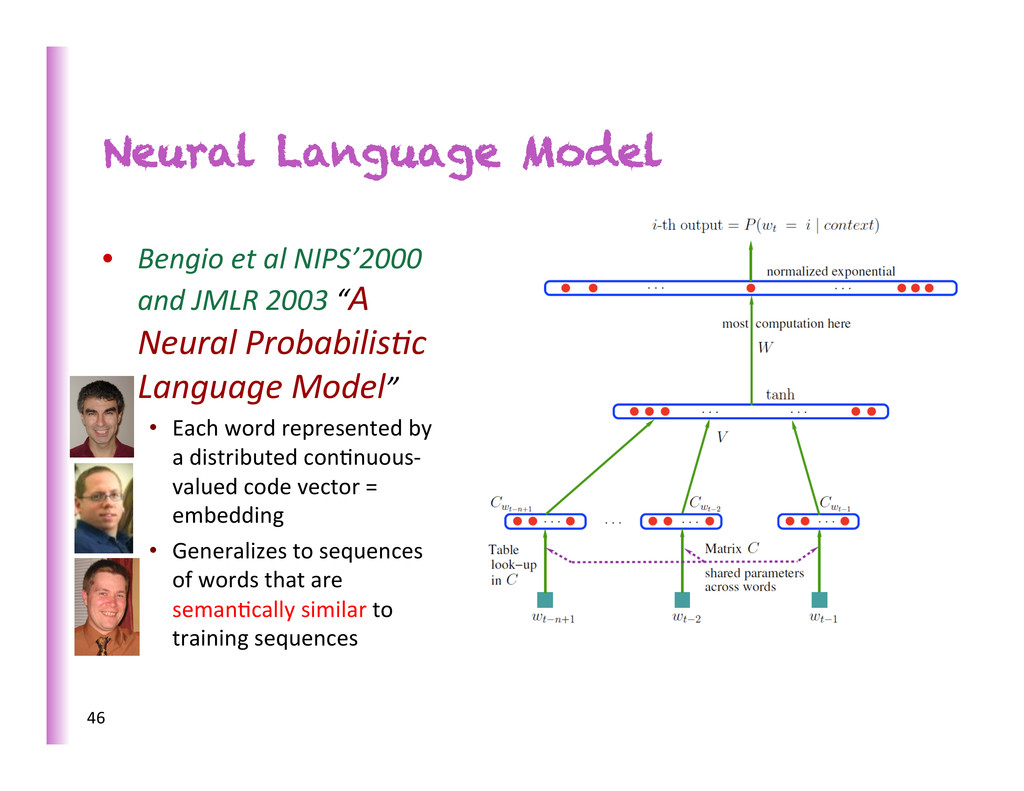
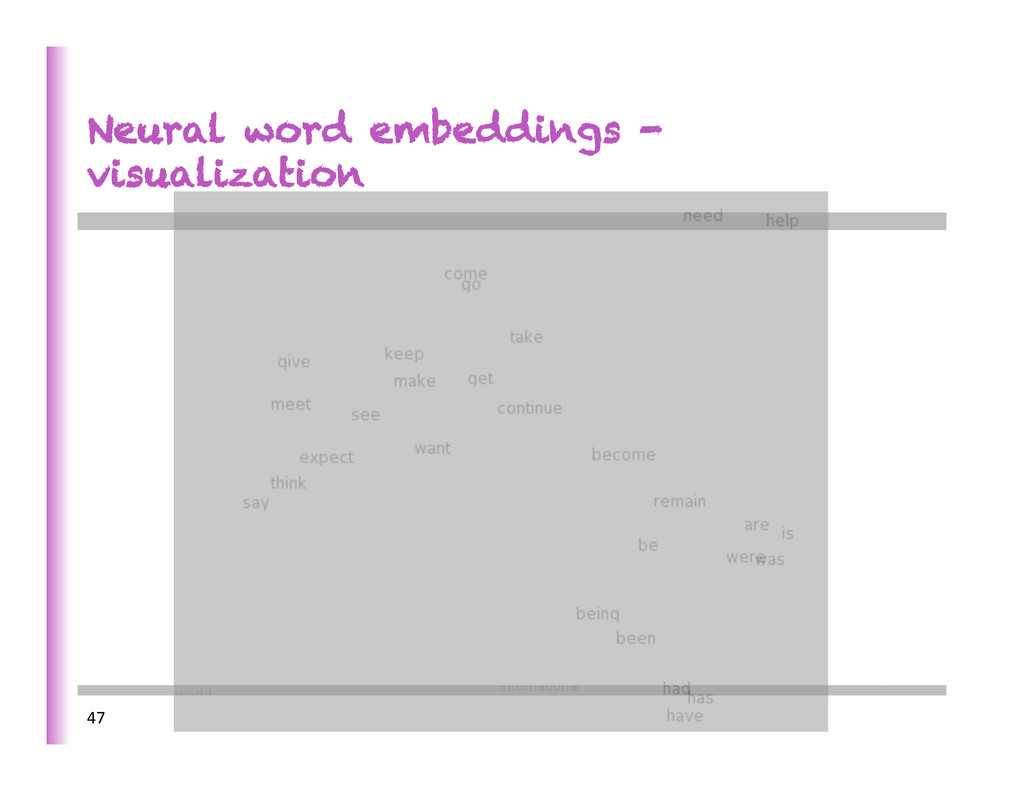
46. Neural Language Model •  Bengio  et  al  NIPS’2000   and  JMLR  2003  “A   Neural  ProbabilisKc   Language  Model”   •  Each  word  represented  by   a  distributed  con8nuous-­‐ valued  code  vector  =   embedding   •  Generalizes  to  sequences   of  words  that  are   seman8cally  similar  to   training  sequences   46  
47. Neural word embeddings - visualization 47  
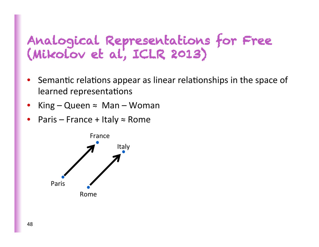
48. Analogical Representations for Free (Mikolov et al, ICLR 2013) •  Seman8c  rela8ons  appear  as  linear  rela8onships  in  the  space  of   learned  representa8ons   •  King  –  Queen  ≈    Man  –  Woman   •  Paris  –  France  +  Italy  ≈  Rome   48   Paris   France   Italy   Rome  
49. More about depth 49  
50. Architecture Depth Depth = 3 Depth = 4
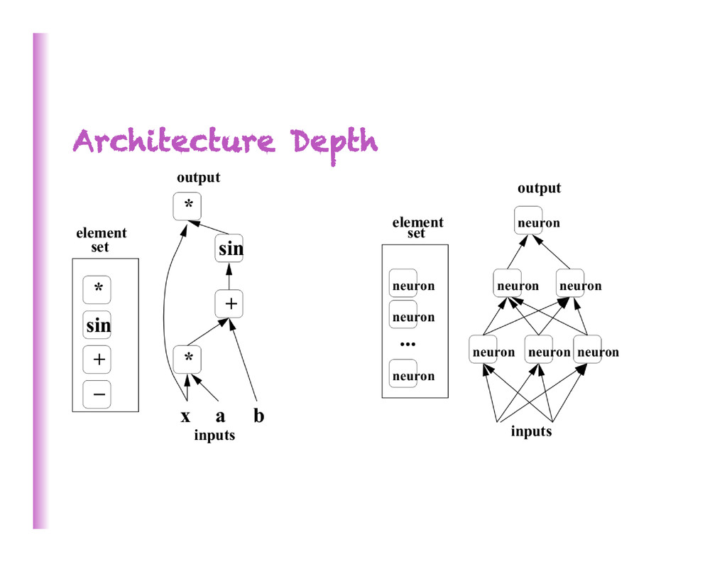
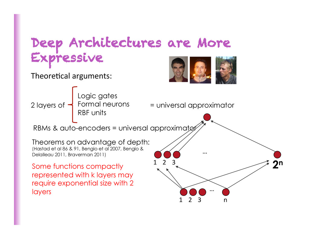
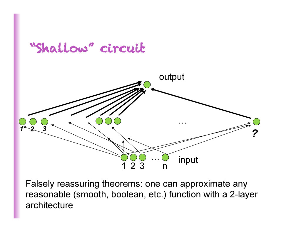
51. Deep Architectures are More Expressive Theore8cal  arguments:   …   1   2   3   2n 1   2   3   …   n   = universal approximator 2 layers of Logic gates Formal neurons RBF units Theorems on advantage of depth: (Hastad et al 86 & 91, Bengio et al 2007, Bengio & Delalleau 2011, Braverman 2011) Some functions compactly represented with k layers may require exponential size with 2 layers RBMs & auto-encoders = universal approximator
52. main sub1 sub2 sub3 subsub1 subsub2 subsub3 subsubsub1 subsubsub2 subsubsub3 “Deep” computer program
53. main subroutine1 includes subsub1 code and subsub2 code and subsubsub1 code “Shallow” computer program subroutine2 includes subsub2 code and subsub3 code and subsubsub3 code and …
54. “Deep” circuit
55. “Shallow” circuit input … ? 1 2 3 … n output Falsely reassuring theorems: one can approximate any reasonable (smooth, boolean, etc.) function with a 2-layer architecture 1 2 3
57. Representation Learning Algorithms Part  2   57  
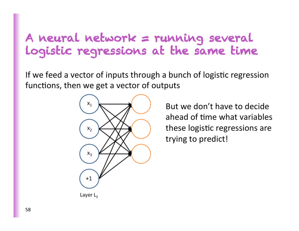
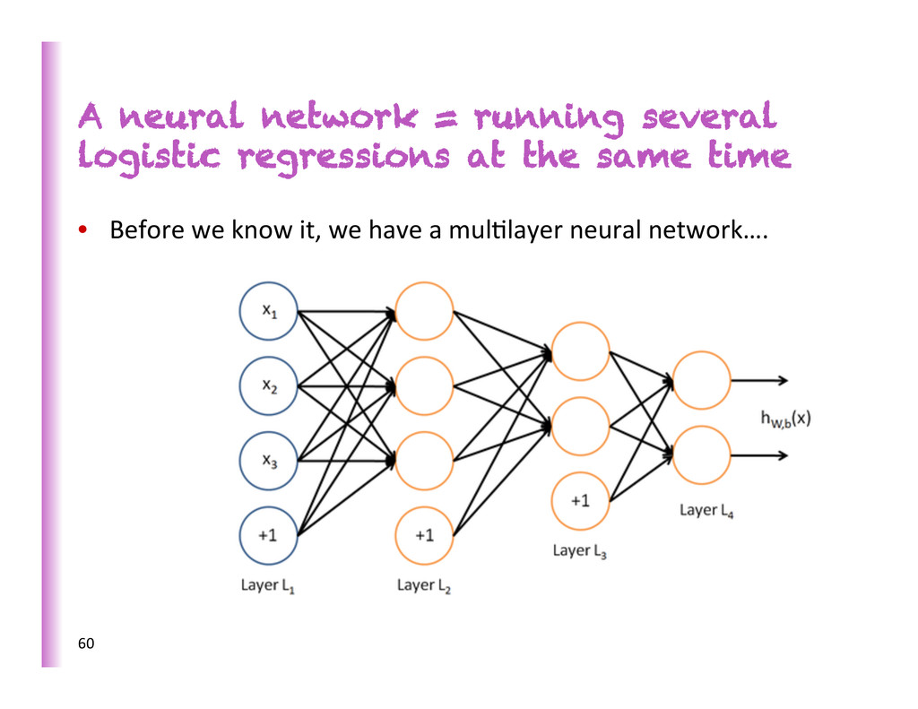
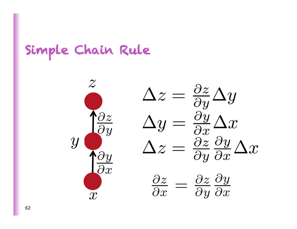
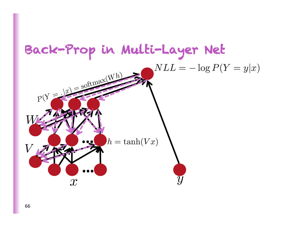
58. A neural network = running several logistic regressions at the same time If  we  feed  a  vector  of  inputs  through  a  bunch  of  logis8c  regression   func8ons,  then  we  get  a  vector  of  outputs   But  we  don’t  have  to  decide   ahead  of  8me  what  variables   these  logis8c  regressions  are   trying  to  predict!   58  
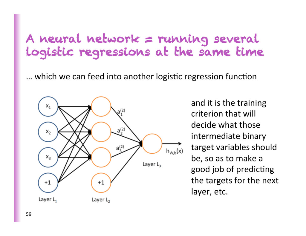
59. A neural network = running several logistic regressions at the same time …  which  we  can  feed  into  another  logis8c  regression  func8on   and  it  is  the  training   criterion  that  will   decide  what  those   intermediate  binary   target  variables  should   be,  so  as  to  make  a   good  job  of  predic8ng   the  targets  for  the  next   layer,  etc.   59  
60. A neural network = running several logistic regressions at the same time •  Before  we  know  it,  we  have  a  mul8layer  neural  network….   60  
61. Back-Prop •  Compute  gradient  of  example-­‐wise  loss  wrt   parameters     •  Simply  applying  the  deriva8ve  chain  rule  wisely   •  If  compuKng  the  loss(example,  parameters)  is  O(n)   computaKon,  then  so  is  compuKng  the  gradient   61  
62. Simple Chain Rule 62  
63. Multiple Paths Chain Rule 63  
64. Multiple Paths Chain Rule - General …   64  
65. Chain Rule in Flow Graph …   …   …   Flow  graph:  any  directed  acyclic  graph    node  =  computa8on  result    arc  =  computa8on  dependency                                                                =  successors  of     65  
66. Back-Prop in Multi-Layer Net …   …   66  
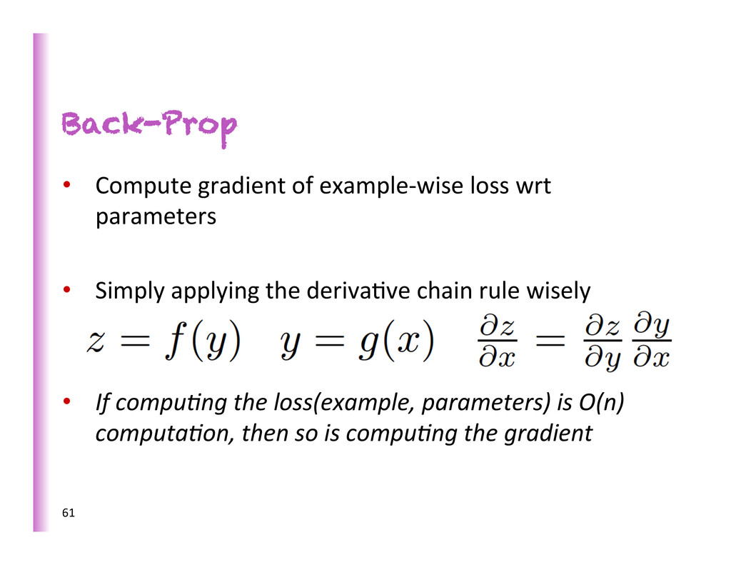
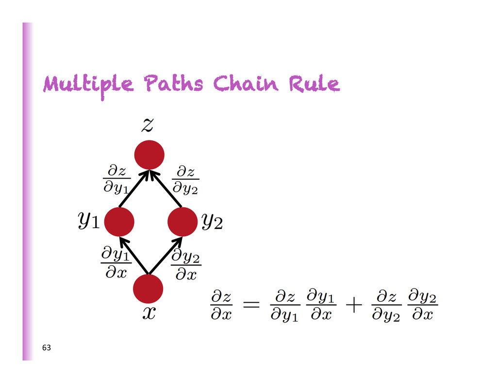
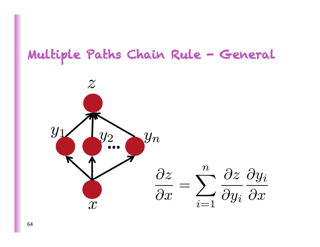
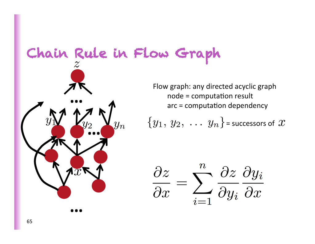
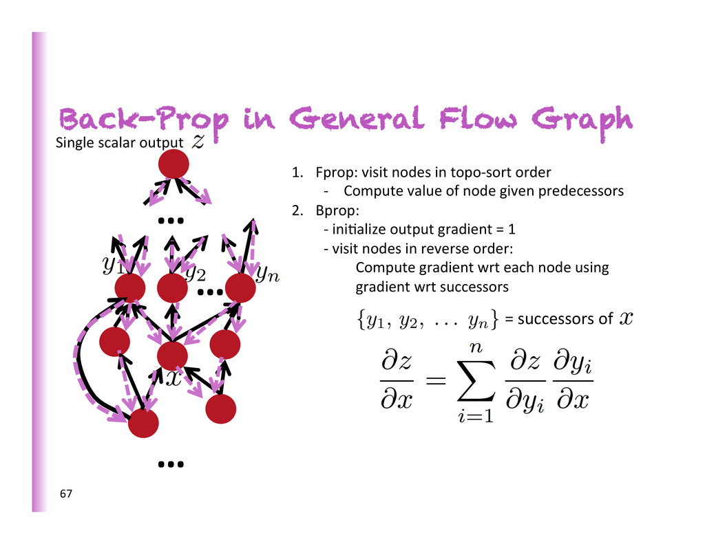
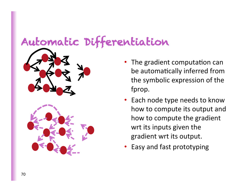
67. Back-Prop in General Flow Graph …   …   …                                                              =  successors  of     1.  Fprop:  visit  nodes  in  topo-­‐sort  order     -­‐  Compute  value  of  node  given  predecessors   2.  Bprop:    -­‐  ini8alize  output  gradient  =  1      -­‐  visit  nodes  in  reverse  order:    Compute  gradient  wrt  each  node  using                  gradient  wrt  successors   Single  scalar  output   67  
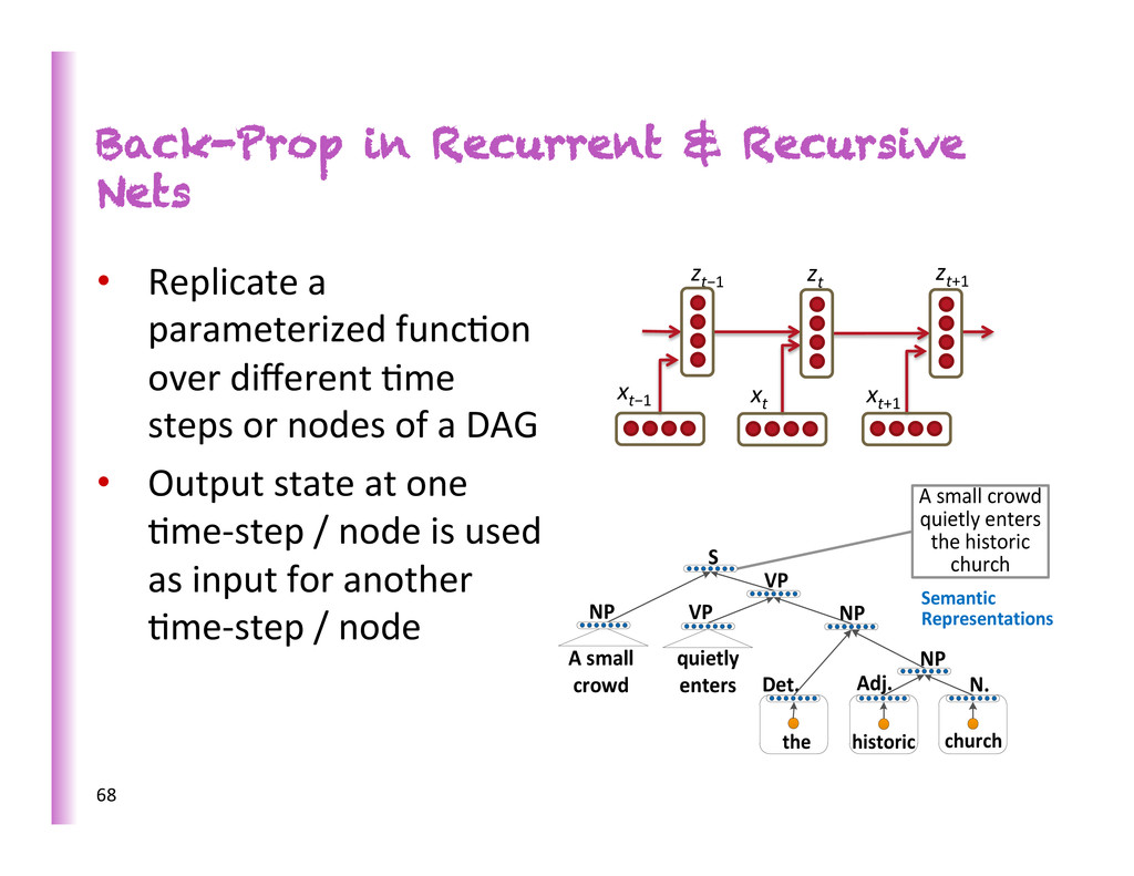
68. Back-Prop in Recurrent & Recursive Nets •  Replicate  a   parameterized  func8on   over  different  8me   steps  or  nodes  of  a  DAG     •  Output  state  at  one   8me-­‐step  /  node  is  used   as  input  for  another   8me-­‐step  /  node   A  small  crowd   quietly  enters   the  historic   church historic the quietly   enters S VP Det. Adj. NP VP A  small   crowd NP NP church N. Semantic     Representations xt−1   xt   xt+1   zt−1   zt   zt+1   68  
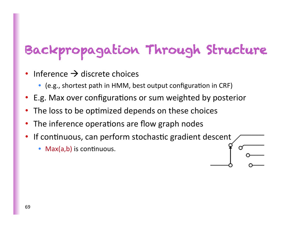
69. Backpropagation Through Structure •  Inference  à  discrete  choices     •  (e.g.,  shortest  path  in  HMM,  best  output  configura8on  in  CRF)   •  E.g.  Max  over  configura8ons  or  sum  weighted  by  posterior   •  The  loss  to  be  op8mized  depends  on  these  choices   •  The  inference  opera8ons  are  flow  graph  nodes   •  If  con8nuous,  can  perform  stochas8c  gradient  descent   •  Max(a,b)  is  con8nuous.   69  
70. Automatic Differentiation •  The  gradient  computa8on  can   be  automa8cally  inferred  from   the  symbolic  expression  of  the   fprop.   •  Each  node  type  needs  to  know   how  to  compute  its  output  and   how  to  compute  the  gradient   wrt  its  inputs  given  the   gradient  wrt  its  output.   •  Easy  and  fast  prototyping   70  
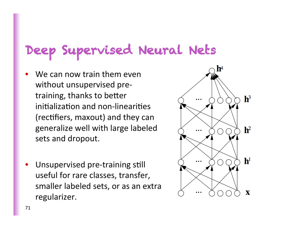
71. Deep Supervised Neural Nets •  We  can  now  train  them  even   without  unsupervised  pre-­‐ training,  thanks  to  beber   ini8aliza8on  and  non-­‐lineari8es   (rec8fiers,  maxout)  and  they  can   generalize  well  with  large  labeled   sets  and  dropout.   •  Unsupervised  pre-­‐training  s8ll   useful  for  rare  classes,  transfer,   smaller  labeled  sets,  or  as  an  extra   regularizer.   71  
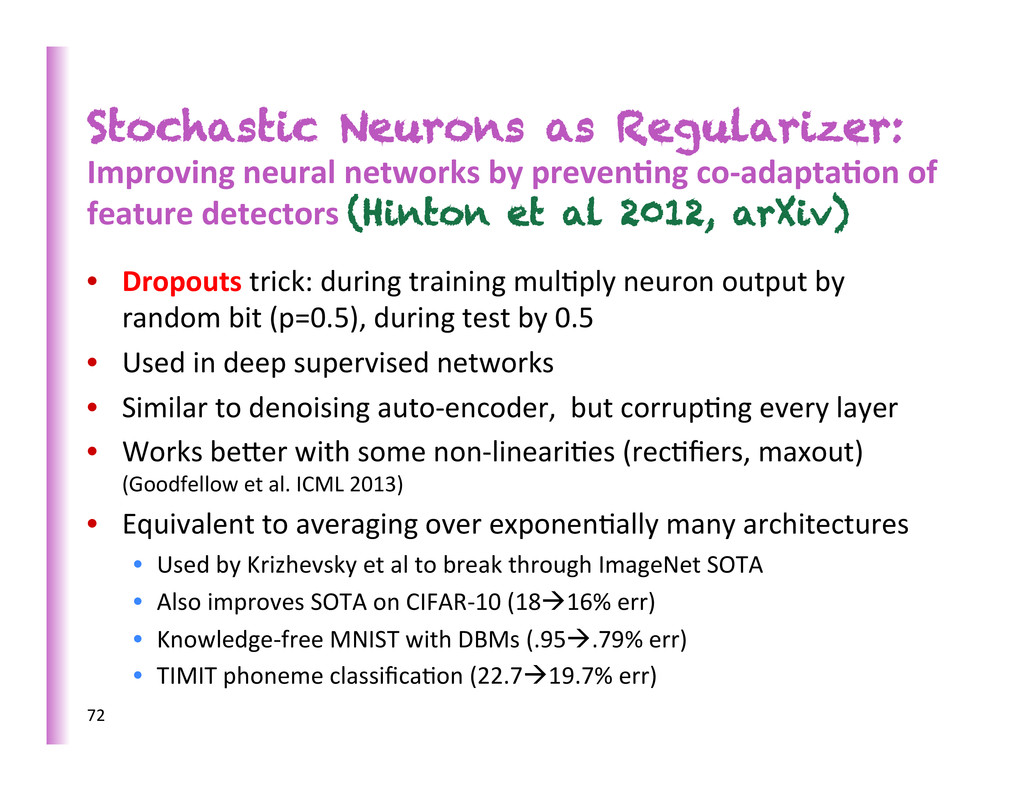
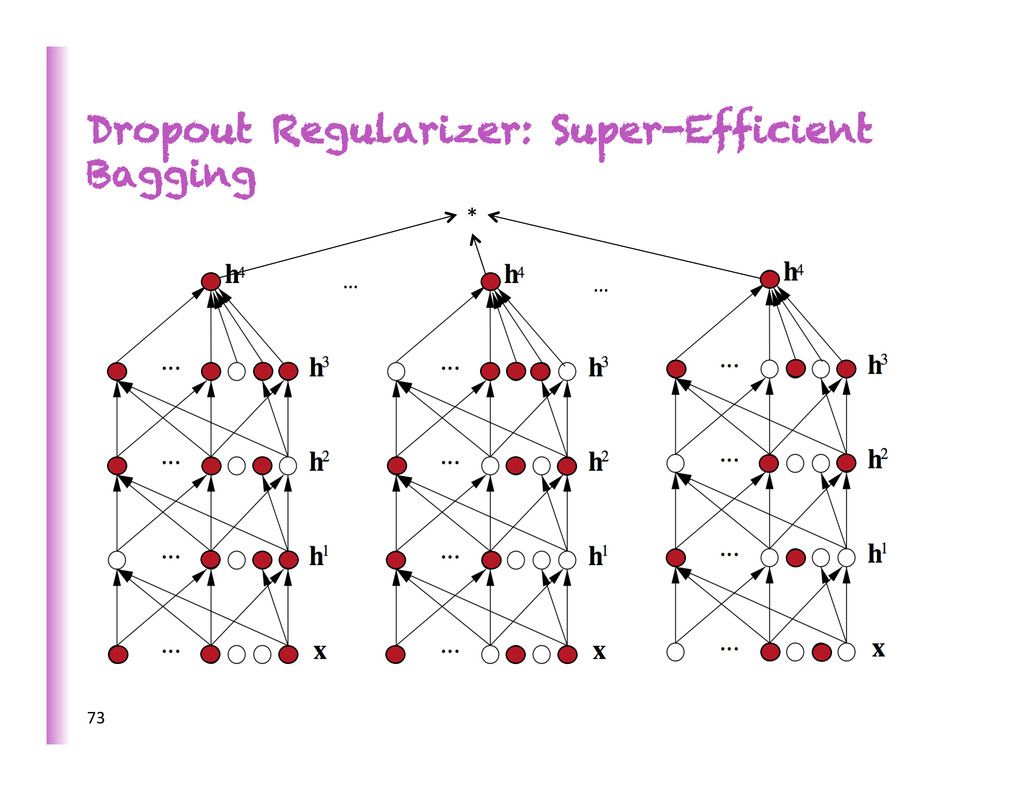
72. Stochastic Neurons as Regularizer: Improving  neural  networks  by  preven0ng  co-­‐adapta0on  of   feature  detectors  (Hinton et al 2012, arXiv) •  Dropouts  trick:  during  training  mul8ply  neuron  output  by   random  bit  (p=0.5),  during  test  by  0.5   •  Used  in  deep  supervised  networks   •  Similar  to  denoising  auto-­‐encoder,    but  corrup8ng  every  layer   •  Works  beber  with  some  non-­‐lineari8es  (rec8fiers,  maxout)             (Goodfellow  et  al.  ICML  2013)   •  Equivalent  to  averaging  over  exponen8ally  many  architectures   •  Used  by  Krizhevsky  et  al  to  break  through  ImageNet  SOTA   •  Also  improves  SOTA  on  CIFAR-­‐10  (18à16%  err)   •  Knowledge-­‐free  MNIST  with  DBMs  (.95à.79%  err)   •  TIMIT  phoneme  classifica8on  (22.7à19.7%  err)   72  
73. Dropout Regularizer: Super-Efficient Bagging 73   *   …   …  
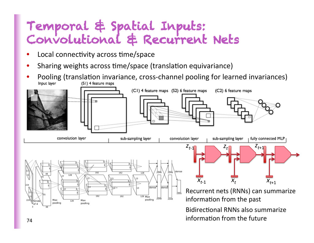
74. Temporal & Spatial Inputs: Convolutional & Recurrent Nets •  Local  connec8vity  across  8me/space   •  Sharing  weights  across  8me/space  (transla8on  equivariance)   •  Pooling  (transla8on  invariance,  cross-­‐channel  pooling  for  learned  invariances)   74   xt-­‐1   xt   xt+1   zt-­‐1   zt   zt+1   Recurrent  nets  (RNNs)  can  summarize   informa8on  from  the  past   Bidirec8onal  RNNs  also  summarize   informa8on  from  the  future  
75. 75   Distributed Representations & Neural Nets: How to do unsupervised training?
76. PCA = Linear Manifold = Linear Auto-Encoder = Linear Gaussian Factors reconstruc8on  error  vector   Linear  manifold   reconstruc8on(x)   x   input  x,  0-­‐mean   features=code=h(x)=W  x   reconstruc8on(x)=WT  h(x)  =  WT  W  x   W  =  principal  eigen-­‐basis  of  Cov(X)   Probabilis8c  interpreta8ons:   1.  Gaussian  with  full   covariance  WT  W+λI   2.  Latent  marginally  iid   Gaussian  factors  h  with       x  =  WT  h  +  noise   76   … code= latent features h … input reconstruction
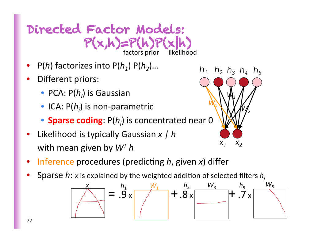
77. Directed Factor Models: P(x,h)=P(h)P(x|h) •  P(h)  factorizes  into  P(h1 )  P(h2 )…   •  Different  priors:   •  PCA:  P(hi )  is  Gaussian   •  ICA:  P(hi )  is  non-­‐parametric   •  Sparse  coding:  P(hi )  is  concentrated  near  0   •  Likelihood  is  typically  Gaussian  x  |  h              with  mean  given  by  WT  h   •  Inference  procedures  (predic8ng  h,  given  x)  differ   •  Sparse  h:  x  is  explained  by  the  weighted  addi8on  of  selected  filters  hi                               =  .9  x                        +  .8  x                      +  .7  x   77   h1 h2 h3 x1 x2 h4 h5 x   W1   W3   W5   h1   h3   h5   W1   W5   W3   factors  prior   likelihood  
78. Sparse autoencoder illustration for images        Natural  Images   Learned  bases:    “Edges”   50 100 150 200 250 300 350 400 450 500 50 100 150 200 250 300 350 400 450 500 50 100 150 200 250 300 350 400 450 500 50 100 150 200 250 300 350 400 450 500 50 100 150 200 250 300 350 400 450 500 50 100 150 200 250 300 350 400 450 500 ≈ 0.8 * + 0.3 * + 0.5 * [h1 ,  …,  h64 ]  =  [0,  0,  …,  0,  0.8,  0,  …,  0,  0.3,  0,  …,  0,  0.5,  0]     (feature  representa8on)     Test  example 78  
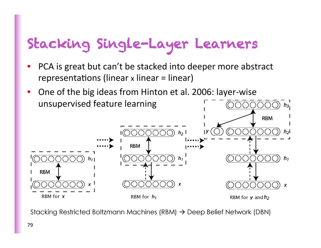
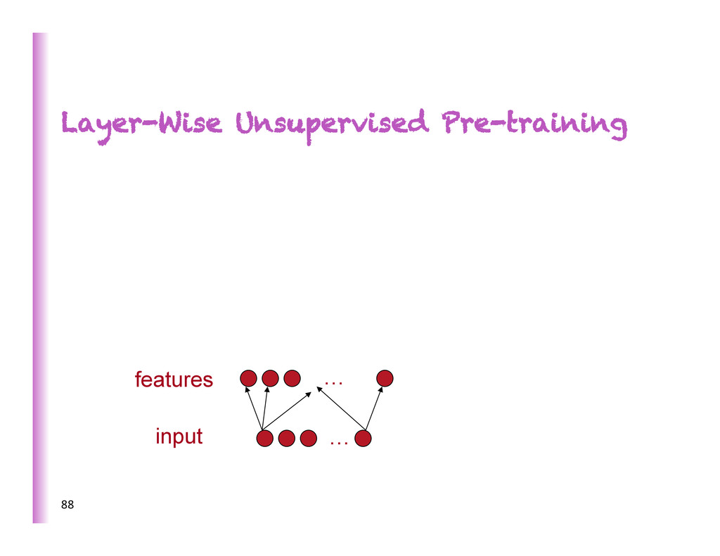
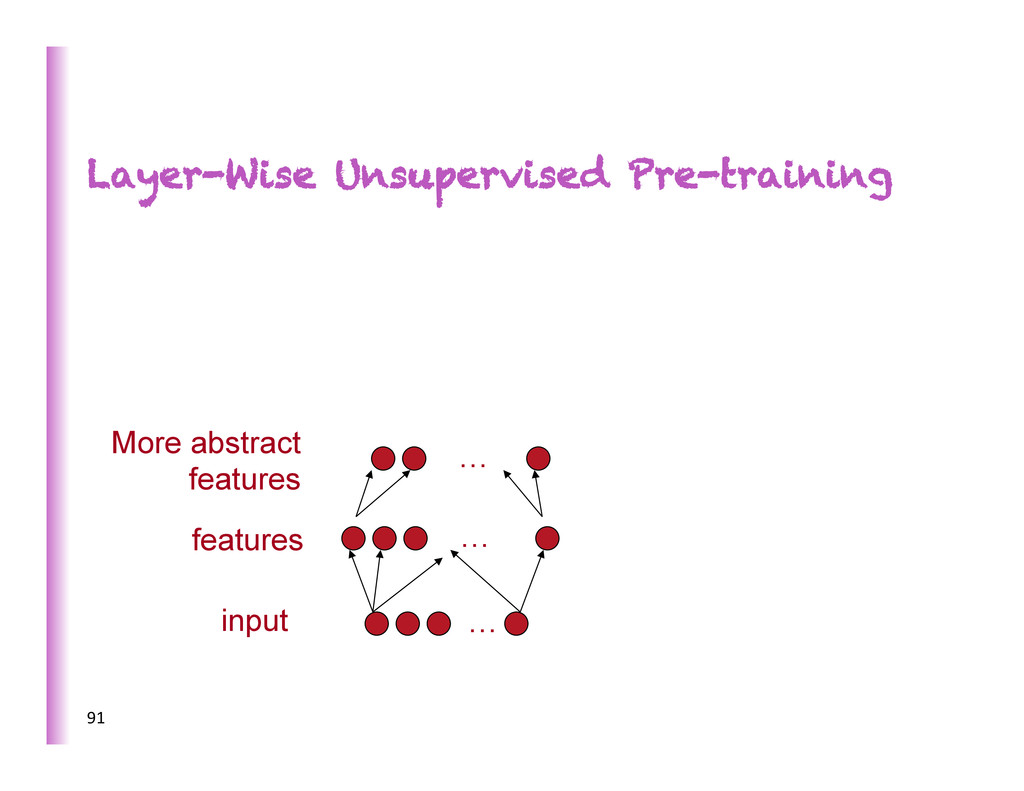
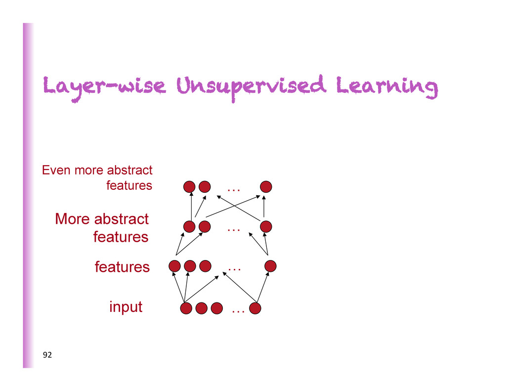
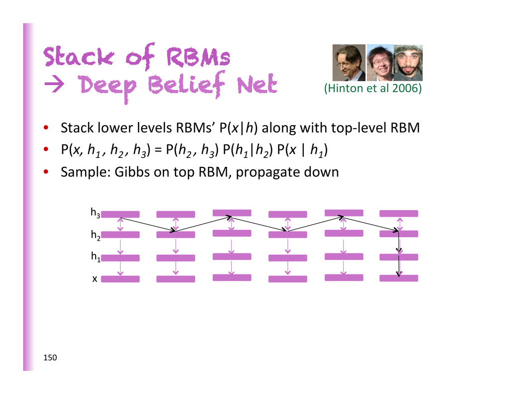
79. Stacking Single-Layer Learners 79   Stacking Restricted Boltzmann Machines (RBM) à Deep Belief Network (DBN) •  PCA  is  great  but  can’t  be  stacked  into  deeper  more  abstract   representa8ons  (linear  x  linear  =  linear)   •  One  of  the  big  ideas  from  Hinton  et  al.  2006:  layer-­‐wise   unsupervised  feature  learning  
80. Effective deep learning first became possible with unsupervised pre-training [Erhan  et  al.,  JMLR  2010]   Purely  supervised  neural  net   With  unsupervised  pre-­‐training   (with  RBMs  and  Denoising  Auto-­‐Encoders)   80  
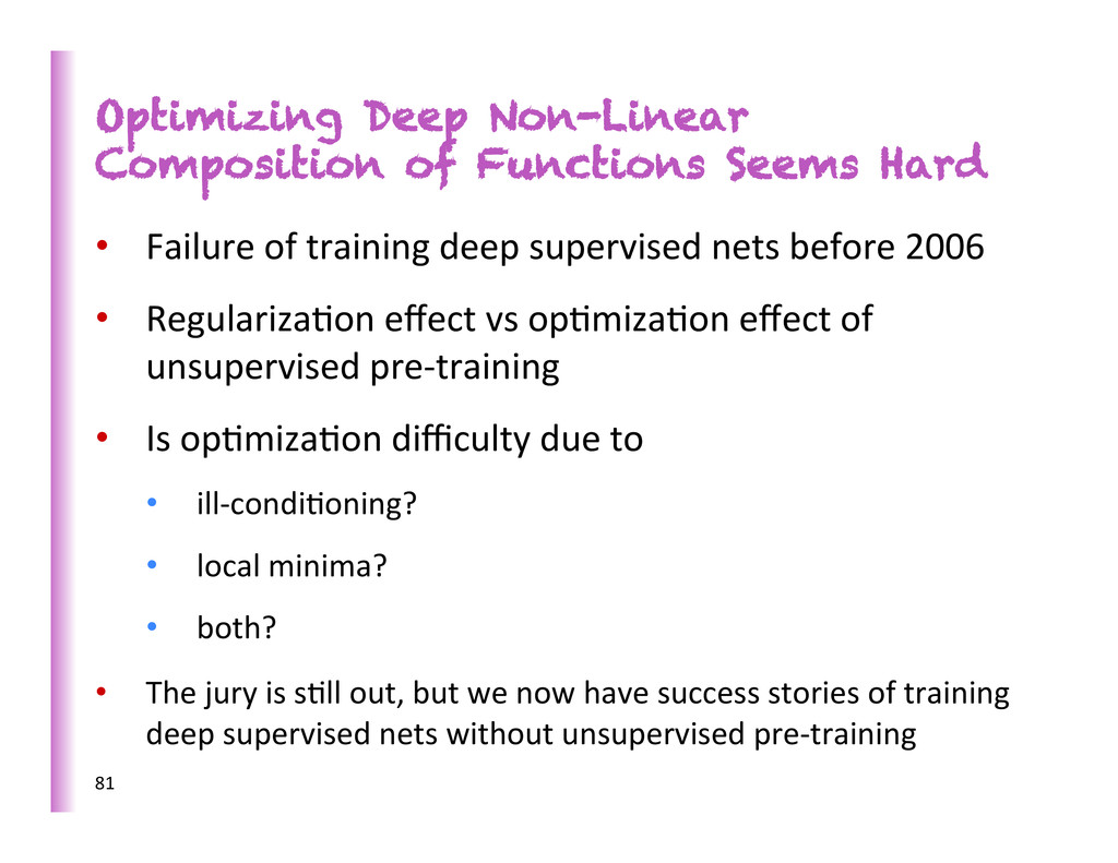
81. Optimizing Deep Non-Linear Composition of Functions Seems Hard 81   •  Failure  of  training  deep  supervised  nets  before  2006   •  Regulariza8on  effect  vs  op8miza8on  effect  of   unsupervised  pre-­‐training   •  Is  op8miza8on  difficulty  due  to     •  ill-­‐condi8oning?   •  local  minima?   •  both?     •  The  jury  is  s8ll  out,  but  we  now  have  success  stories  of  training   deep  supervised  nets  without  unsupervised  pre-­‐training  
82. Initial Examples Matter More (critical period?) Vary 10% of the training set at the beginning, middle, or end of the online sequence. Measure the effect on learned function. 82  
83. Order & Selection of Examples Matters (Bengio,  Louradour,  Collobert  &  Weston,  ICML’2009)        A   • Curriculum  learning     •  (Bengio  et  al  2009,  Krueger  &  Dayan  2009)       •  Start  with  easier  examples   •  Faster  convergence  to  a  beber  local   minimum  in  deep  architectures   !"#$% &% &"!$% '% $''% ('''% ($''% !"#$%&'()'*+,)-"%./) 01!!1"')) 23.&,*4) !"#$% &% &"!$% &"$% !"#$%&'()'*+,)-"%./) 01!!1"')) )*++,)*-*.% /01)*++,)*-*.% 83  
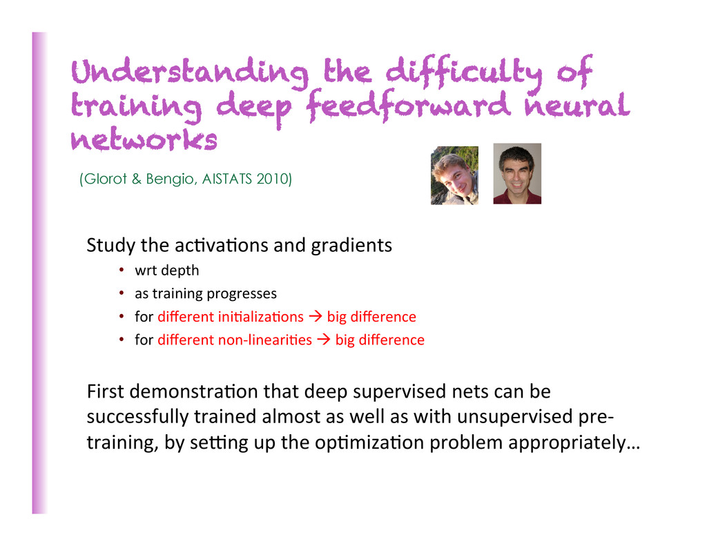
84. Understanding the difficulty of training deep feedforward neural networks (Glorot & Bengio, AISTATS 2010) Study  the  ac8va8ons  and  gradients   •  wrt  depth   •  as  training  progresses   •  for  different  ini8aliza8ons  à  big  difference   •  for  different  non-­‐lineari8es  à  big  difference   First  demonstra8on  that  deep  supervised  nets  can  be   successfully  trained  almost  as  well  as  with  unsupervised  pre-­‐ training,  by  se€ng  up  the  op8miza8on  problem  appropriately…  
85. Layer-wise Unsupervised Learning … input 85  
86. Layer-Wise Unsupervised Pre-training … … input features 86  
87. Layer-Wise Unsupervised Pre-training … … … input features reconstruction of input = ? … input 87  
88. Layer-Wise Unsupervised Pre-training … … input features 88  
89. Layer-Wise Unsupervised Pre-training … … input features … More abstract features 89  
90. … … input features … More abstract features reconstruction of features = ? … … … … Layer-Wise Unsupervised Pre-training Layer-wise Unsupervised Learning 90  
91. … … input features … More abstract features Layer-Wise Unsupervised Pre-training 91  
92. … … input features … More abstract features … Even more abstract features Layer-wise Unsupervised Learning 92  
93. … … input features … More abstract features … Even more abstract features Output f(X) six Target Y two! = ? Supervised Fine-Tuning •  Addi8onal  hypothesis:  features  good  for  P(x)  good  for  P(y|x)   93  
94. Restricted Boltzmann Machines 94  
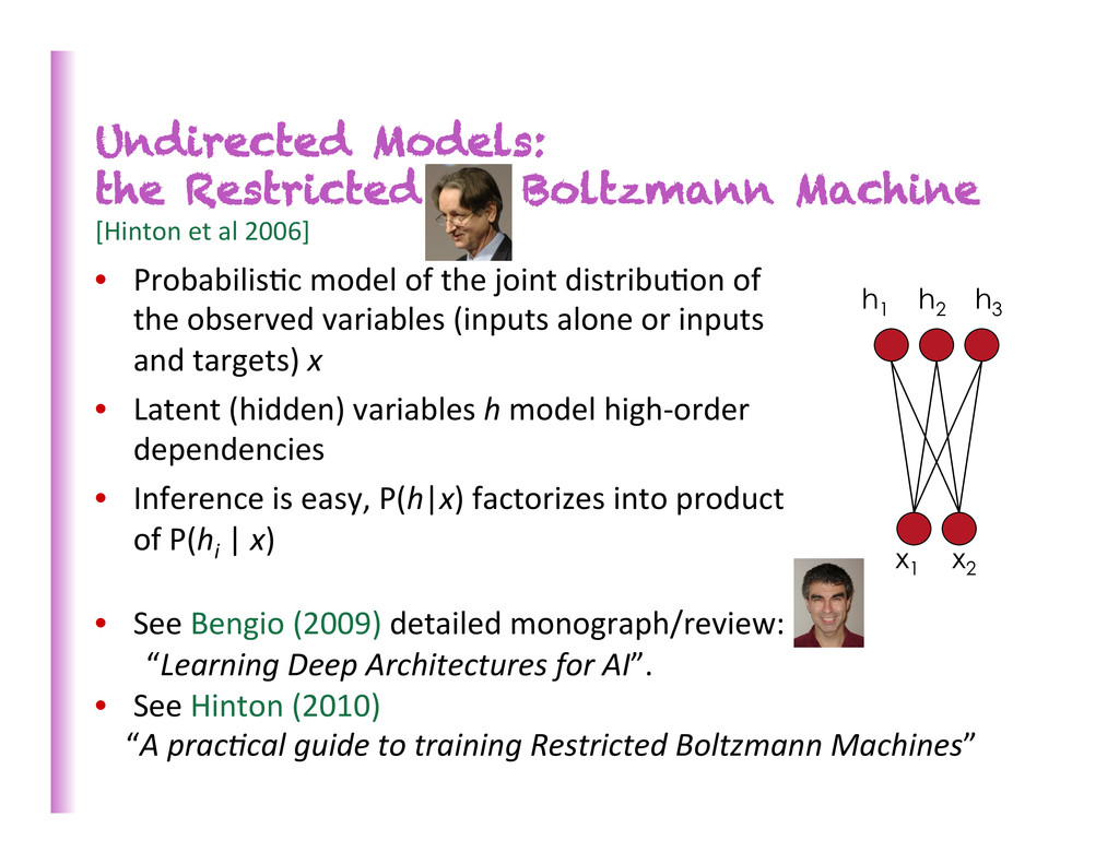
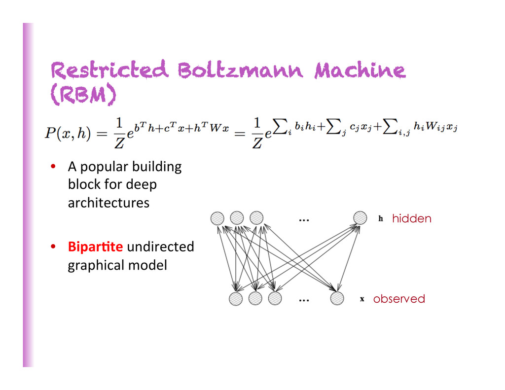
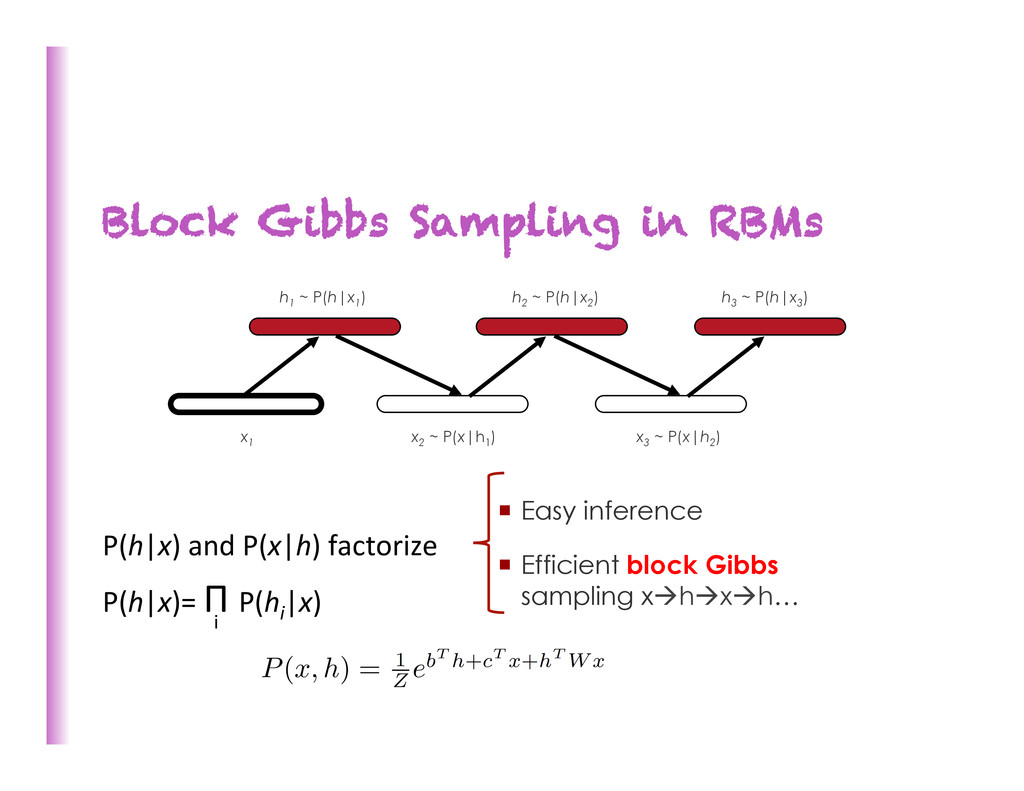
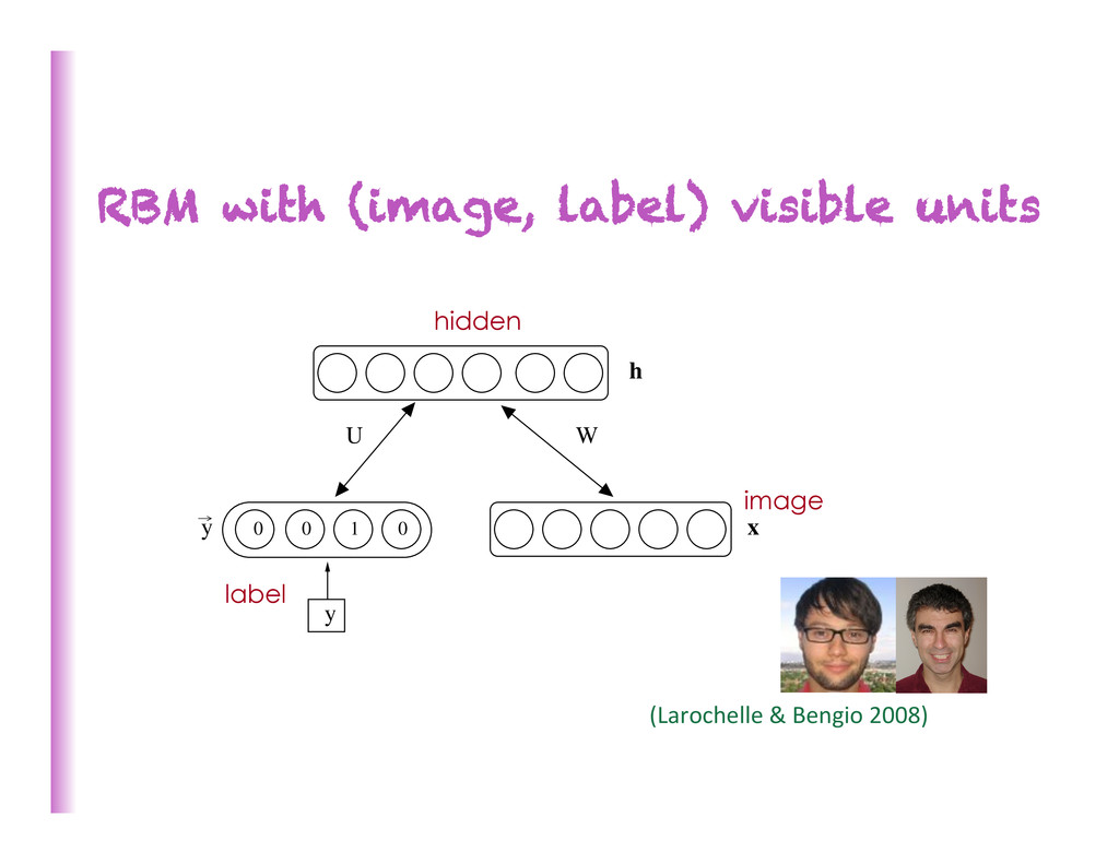
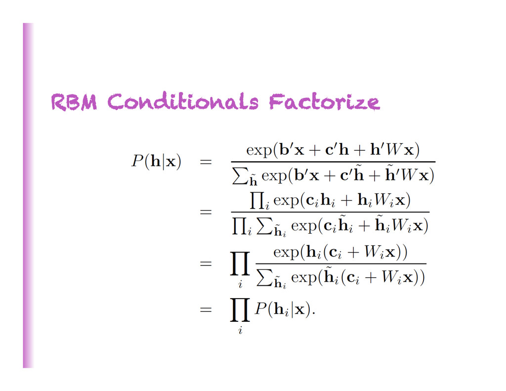
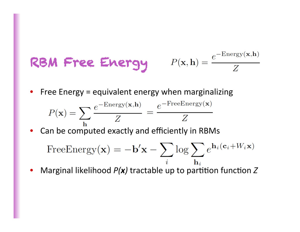
95. •  See  Bengio  (2009)  detailed  monograph/review:        “Learning  Deep  Architectures  for  AI”.   •  See  Hinton  (2010)            “A  pracKcal  guide  to  training  Restricted  Boltzmann  Machines”   Undirected Models: the Restricted Boltzmann Machine [Hinton  et  al  2006]   •  Probabilis8c  model  of  the  joint  distribu8on  of   the  observed  variables  (inputs  alone  or  inputs   and  targets)  x   •  Latent  (hidden)  variables  h  model  high-­‐order   dependencies   •  Inference  is  easy,  P(h|x)  factorizes  into  product   of  P(hi  |  x)     h1 h2 h3 x1 x2
96. Boltzmann Machines & MRFs •  Boltzmann  machines:        (Hinton  84)     •  Markov  Random  Fields:                                                                                                                                             ¡  More  interes8ng  with  latent  variables!                                                                                                                                                                                                                                                       SoZ  constraint  /  probabilis8c  statement   Undirected   graphical   models  
97. Restricted Boltzmann Machine (RBM) •  A  popular  building   block  for  deep   architectures     •  Bipar0te  undirected   graphical  model   observed hidden
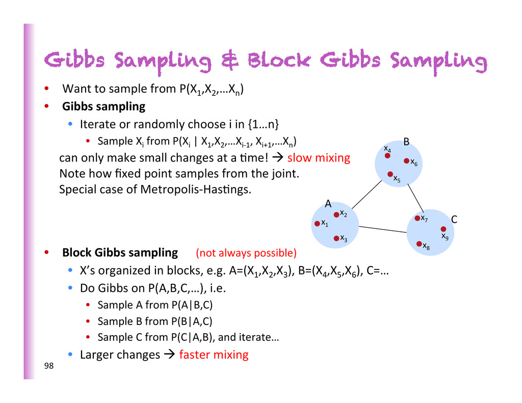
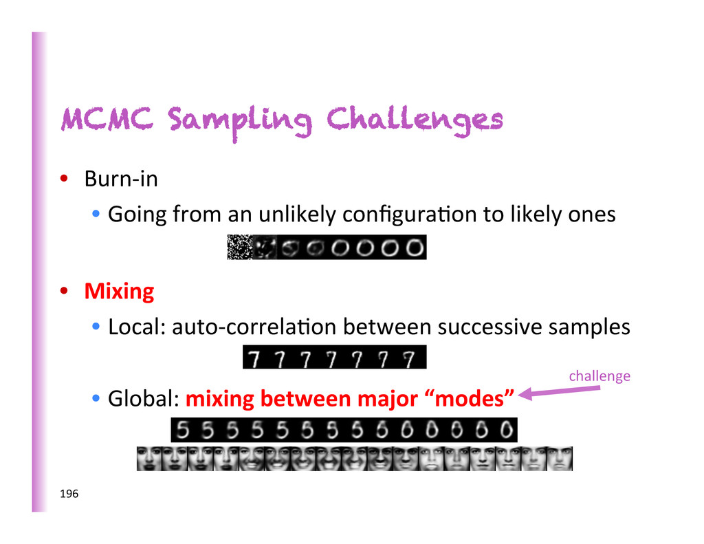
98. Gibbs Sampling & Block Gibbs Sampling •  Want  to  sample  from  P(X1 ,X2 ,…Xn )   •  Gibbs  sampling   •  Iterate  or  randomly  choose  i  in  {1…n}   •  Sample  Xi  from  P(Xi  |  X1 ,X2 ,…Xi-­‐1 ,  Xi+1 ,…Xn )            can  only  make  small  changes  at  a  8me!  à  slow  mixing            Note  how  fixed  point  samples  from  the  joint.              Special  case  of  Metropolis-­‐Has8ngs.         •  Block  Gibbs  sampling            (not  always  possible)   •  X’s  organized  in  blocks,  e.g.  A=(X1 ,X2 ,X3 ),  B=(X4 ,X5 ,X6 ),  C=…   •  Do  Gibbs  on  P(A,B,C,…),  i.e.   •  Sample  A  from  P(A|B,C)         •  Sample  B  from  P(B|A,C)   •  Sample  C  from  P(C|A,B),  and  iterate…   •  Larger  changes  à  faster  mixing   98   A   B   C   x9   x8   x7   x1   x2   x3   x4   x5   x6  
99. Block Gibbs Sampling in RBMs P(h|x)  and  P(x|h)  factorize   P(h|x)=  Π  P(hi |x)   h1 ~ P(h|x1 ) x2 ~ P(x|h1 ) x3 ~ P(x|h2 ) x1 h2 ~ P(h|x2 ) h3 ~ P(h|x3 ) ¡  Easy inference ¡  Efficient block Gibbs sampling xàhàxàh… i  
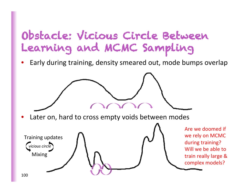
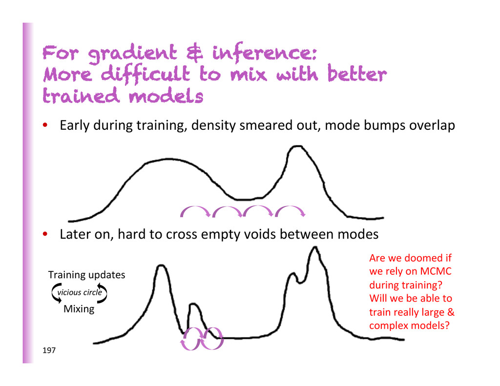
100. Obstacle: Vicious Circle Between Learning and MCMC Sampling •  Early  during  training,  density  smeared  out,  mode  bumps  overlap   •  Later  on,  hard  to  cross  empty  voids  between  modes   100   Are  we  doomed  if   we  rely  on  MCMC   during  training?   Will  we  be  able  to   train  really  large  &   complex  models?     Training  updates   Mixing   vicious  circle  
101. RBM with (image, label) visible units label hidden y 0 0 0 1 y x h U W image (Larochelle  &  Bengio  2008)  
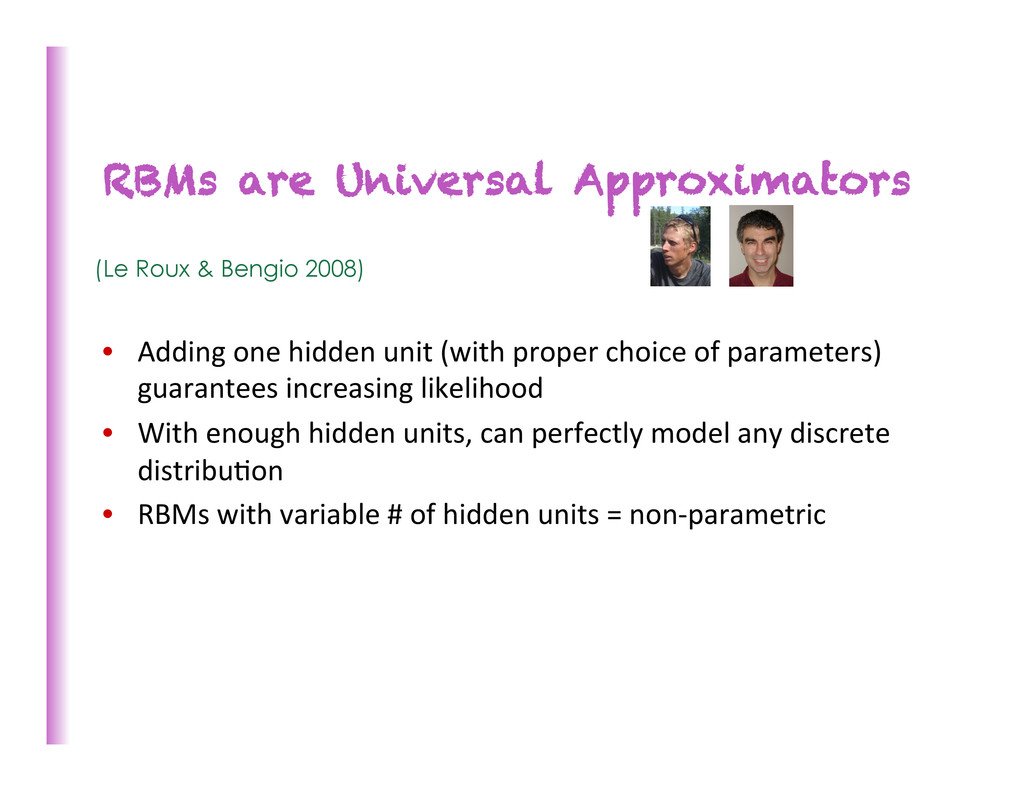
102. RBMs are Universal Approximators •  Adding  one  hidden  unit  (with  proper  choice  of  parameters)   guarantees  increasing  likelihood     •  With  enough  hidden  units,  can  perfectly  model  any  discrete   distribu8on   •  RBMs  with  variable  #  of  hidden  units  =  non-­‐parametric   (Le Roux & Bengio 2008)
103. RBM Conditionals Factorize
104. RBM Energy Gives Binomial Neurons
105. •  Free  Energy  =  equivalent  energy  when  marginalizing       •  Can  be  computed  exactly  and  efficiently  in  RBMs     •  Marginal  likelihood  P(x)  tractable  up  to  par88on  func8on  Z   RBM Free Energy
106. Energy-Based Models Gradient
107. Boltzmann Machine Gradient •  Gradient  has  two  components:   ¡  In  RBMs,  easy  to  sample  or  sum  over  h|x   ¡  Difficult  part:  sampling  from  P(x),  typically  with  a  Markov  chain   lnegative phasez lpositive phasez
108. Positive & Negative Samples •  Observed (+) examples push the energy down •  Generated / dream / fantasy (-) samples / particles push the energy up X+ X- Equilibrium:  E[gradient]  =  0  
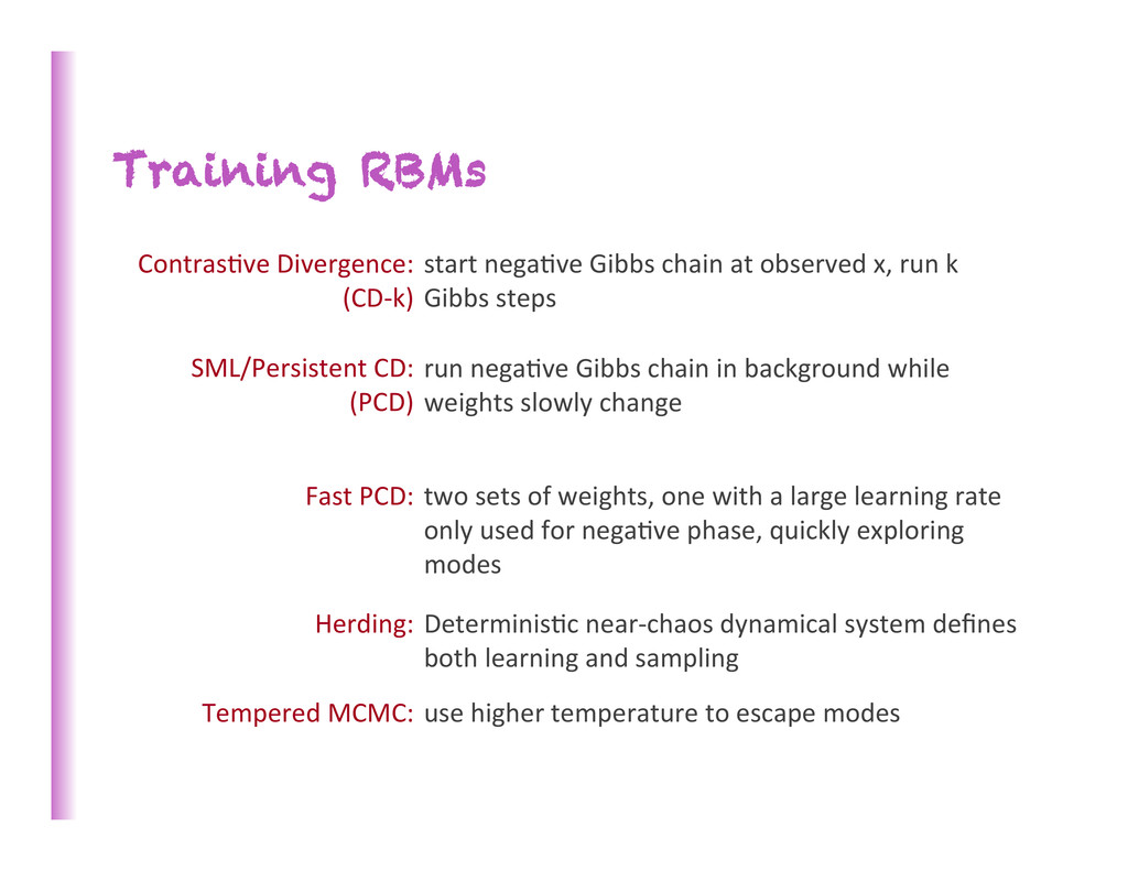
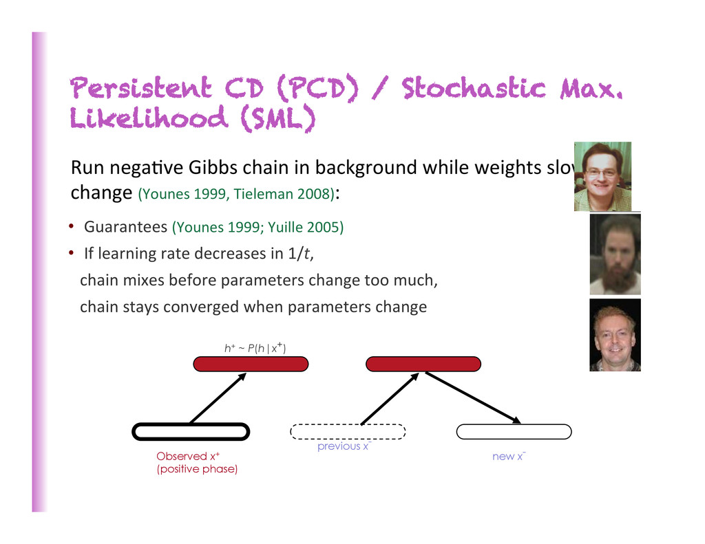
109. Training RBMs Contras8ve  Divergence:     (CD-­‐k)   start  nega8ve  Gibbs  chain  at  observed  x,  run  k   Gibbs  steps     SML/Persistent  CD:   (PCD)     run  nega8ve  Gibbs  chain  in  background  while   weights  slowly  change   Fast  PCD:  two  sets  of  weights,  one  with  a  large  learning  rate   only  used  for  nega8ve  phase,  quickly  exploring   modes   Herding:  Determinis8c  near-­‐chaos  dynamical  system  defines   both  learning  and  sampling   Tempered  MCMC:  use  higher  temperature  to  escape  modes  
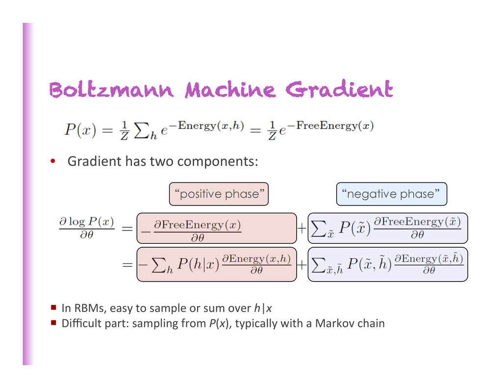
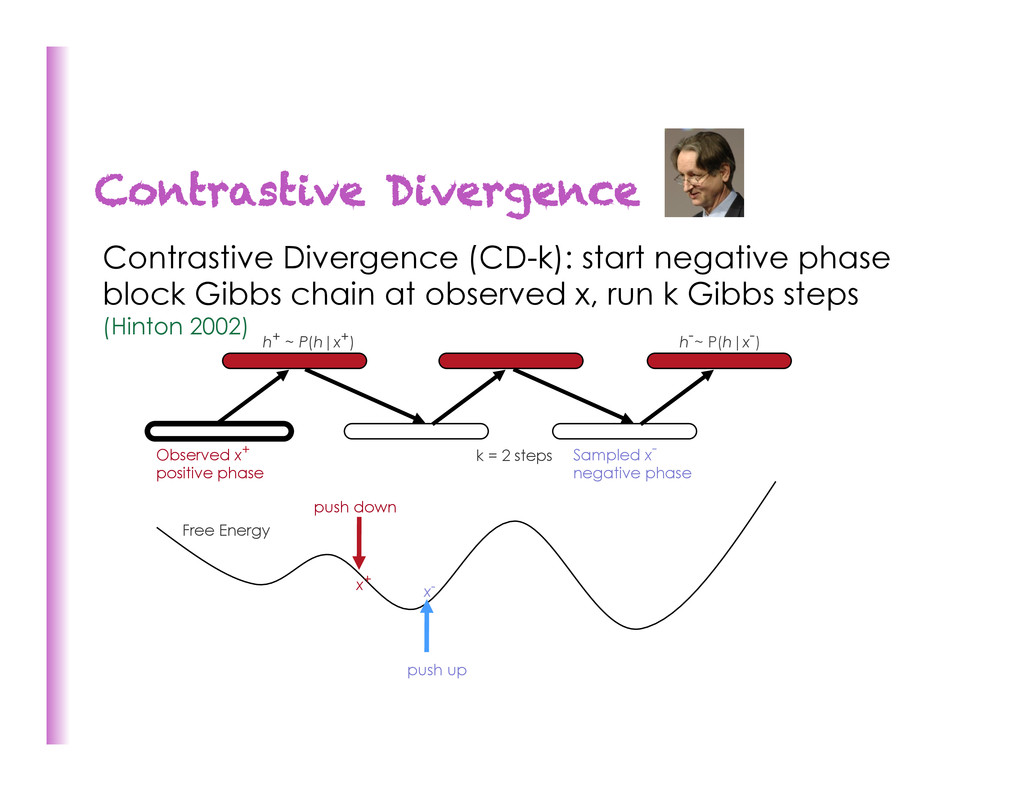
110. Contrastive Divergence Contrastive Divergence (CD-k): start negative phase block Gibbs chain at observed x, run k Gibbs steps (Hinton 2002) Sampled x- negative phase Observed x+ positive phase h+ ~ P(h|x+) h-~ P(h|x-) k = 2 steps x+ x- Free Energy push down push up
111. Persistent CD (PCD) / Stochastic Max. Likelihood (SML) Run  nega8ve  Gibbs  chain  in  background  while  weights  slowly   change  (Younes  1999,  Tieleman  2008):       Observed x+ (positive phase) new x- h+ ~ P(h|x+) previous x- •  Guarantees  (Younes  1999;  Yuille  2005)   •  If  learning  rate  decreases  in  1/t,          chain  mixes  before  parameters  change  too  much,          chain  stays  converged  when  parameters  change  
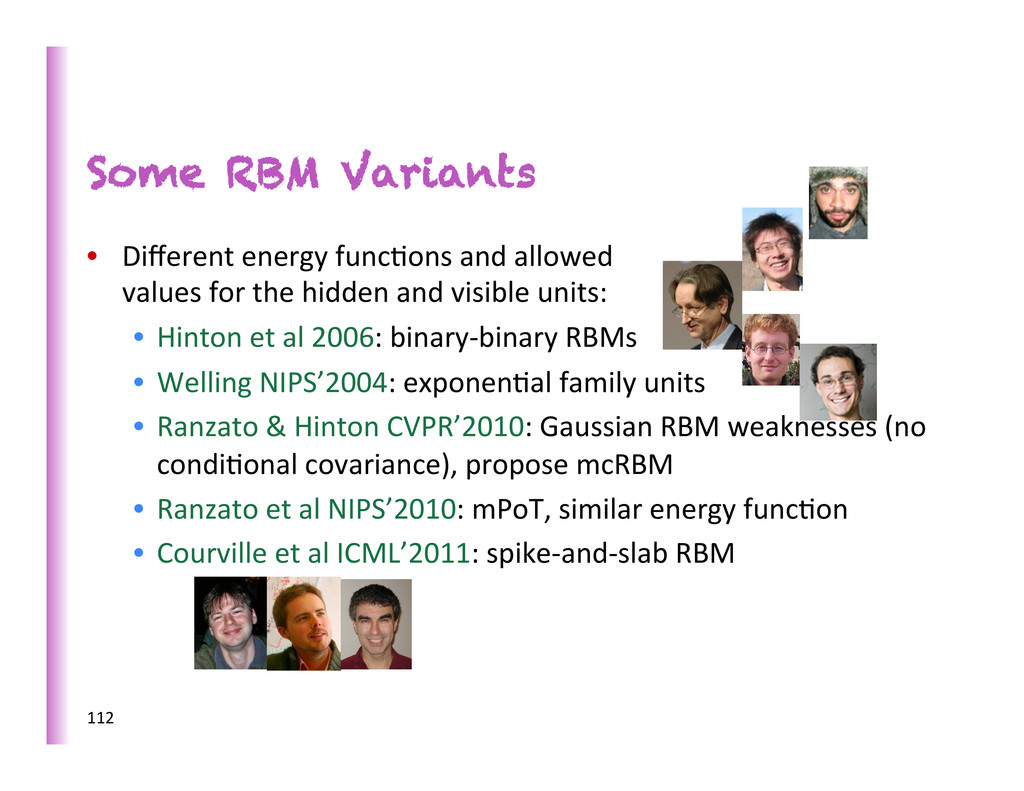
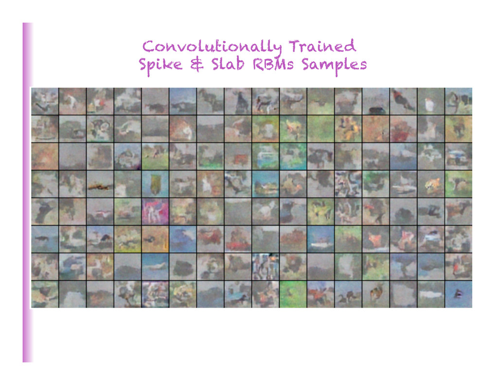
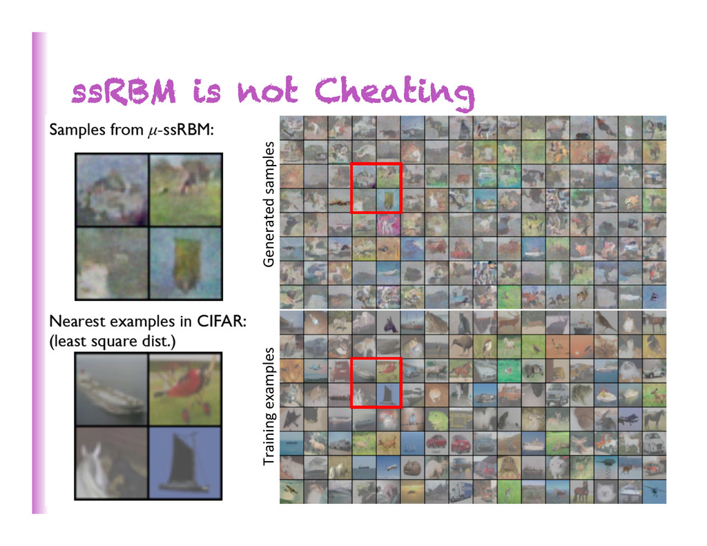
112. Some RBM Variants •  Different  energy  func8ons  and  allowed                   values  for  the  hidden  and  visible  units:   •  Hinton  et  al  2006:  binary-­‐binary  RBMs   •  Welling  NIPS’2004:  exponen8al  family  units   •  Ranzato  &  Hinton  CVPR’2010:  Gaussian  RBM  weaknesses  (no   condi8onal  covariance),  propose  mcRBM   •  Ranzato  et  al  NIPS’2010:  mPoT,  similar  energy  func8on   •  Courville  et  al  ICML’2011:  spike-­‐and-­‐slab  RBM     112  
113. Convolutionally Trained Spike & Slab RBMs Samples
114. ssRBM is not Cheating Generated  samples   Training  examples  
115. Auto-Encoders & Variants: Learning a computational graph 115  
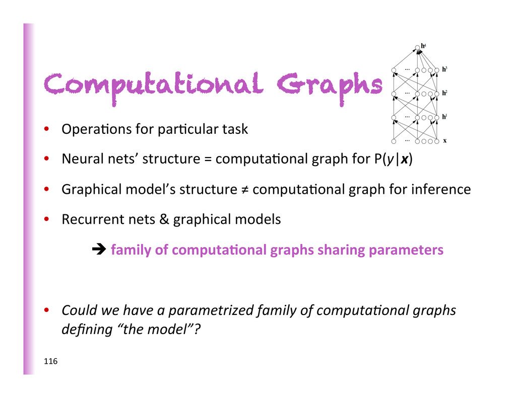
116. Computational Graphs •  Opera8ons  for  par8cular  task   •  Neural  nets’  structure  =  computa8onal  graph  for  P(y|x)   •  Graphical  model’s  structure  ≠  computa8onal  graph  for  inference   •  Recurrent  nets  &  graphical  models      è  family  of  computa0onal  graphs  sharing  parameters   •  Could  we  have  a  parametrized  family  of  computaKonal  graphs   defining  “the  model”?   116  
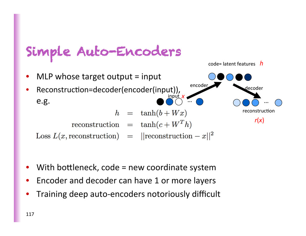
117. •  MLP  whose  target  output  =  input   •  Reconstruc8on=decoder(encoder(input)),                               e.g.     •  With  bobleneck,  code  =  new  coordinate  system   •  Encoder  and  decoder  can  have  1  or  more  layers   •  Training  deep  auto-­‐encoders  notoriously  difficult     Simple Auto-Encoders …    code=  latent  features   …    encoder    decoder    input    reconstruc8on   117   r(x)   x   h  
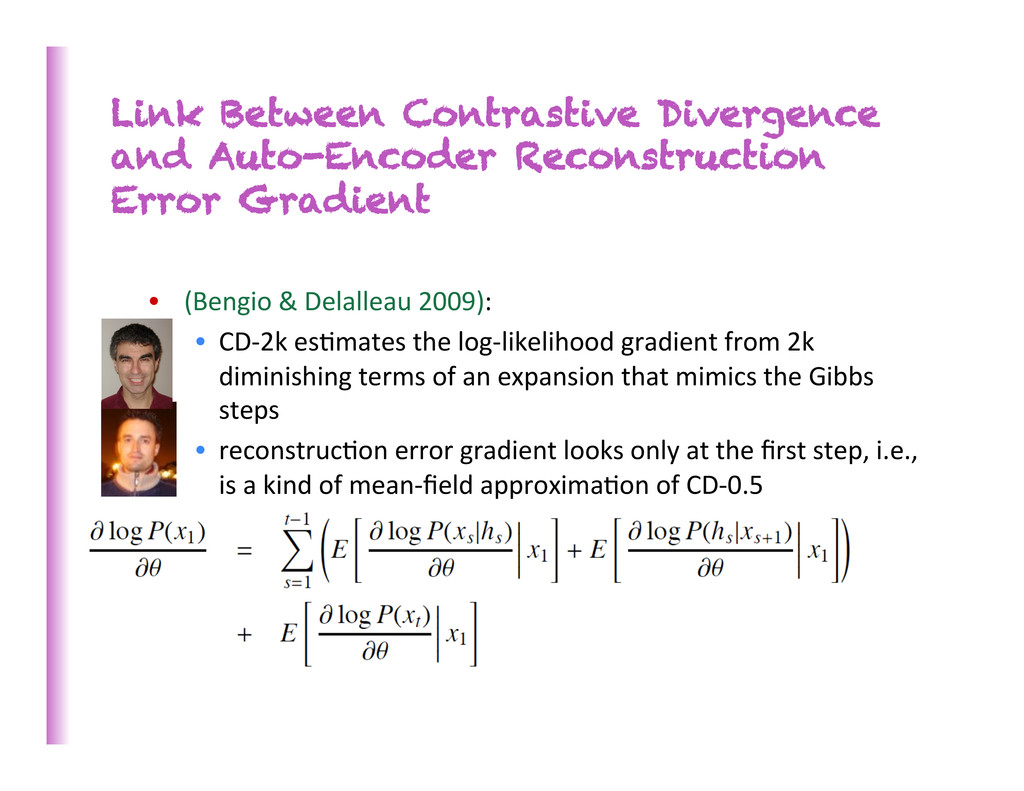
118. Link Between Contrastive Divergence and Auto-Encoder Reconstruction Error Gradient •  (Bengio  &  Delalleau  2009):     •  CD-­‐2k  es8mates  the  log-­‐likelihood  gradient  from  2k   diminishing  terms  of  an  expansion  that  mimics  the  Gibbs   steps   •  reconstruc8on  error  gradient  looks  only  at  the  first  step,  i.e.,   is  a  kind  of  mean-­‐field  approxima8on  of  CD-­‐0.5  
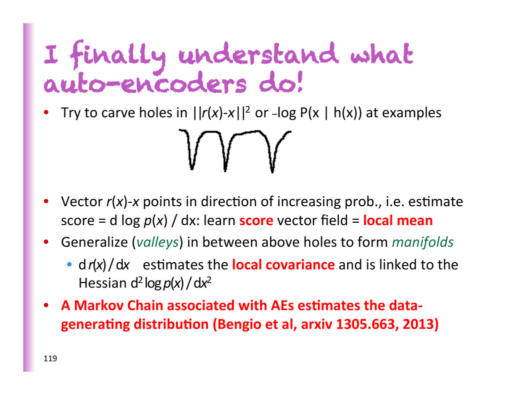
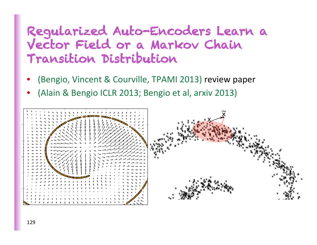
119. I finally understand what auto-encoders do! •  Try  to  carve  holes  in  ||r(x)-­‐x||2    or  –log  P(x  |  h(x))  at  examples   •  Vector  r(x)-­‐x  points  in  direc8on  of  increasing  prob.,  i.e.  es8mate   score  =  d  log  p(x)  /  dx:  learn  score  vector  field  =  local  mean   •  Generalize  (valleys)  in  between  above  holes  to  form  manifolds   •  d  r(x)  /  dx        es8mates  the  local  covariance  and  is  linked  to  the   Hessian  d2  log  p(x)  /  dx2   •  A  Markov  Chain  associated  with  AEs  es0mates  the  data-­‐ genera0ng  distribu0on  (Bengio  et  al,  arxiv  1305.663,  2013)     119  
120. Stacking Auto-Encoders 120   Auto-­‐encoders  can  be  stacked  successfully  (Bengio  et  al  NIPS’2006)  to  form   highly  non-­‐linear  representa8ons,  which  with  fine-­‐tuning  overperformed   purely  supervised  MLPs    
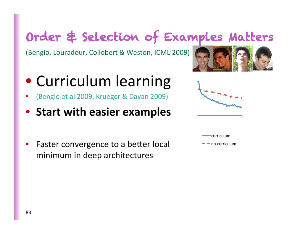
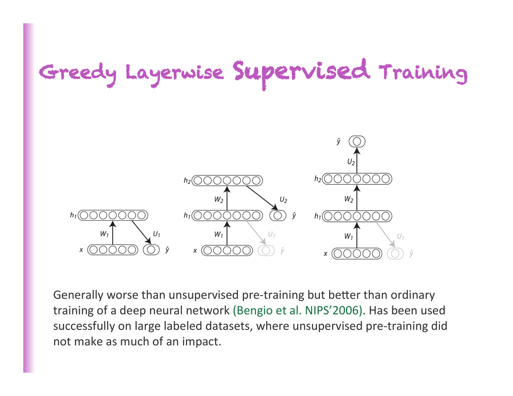
121. Greedy Layerwise Supervised Training Generally  worse  than  unsupervised  pre-­‐training  but  beber  than  ordinary   training  of  a  deep  neural  network  (Bengio  et  al.  NIPS’2006).  Has  been  used   successfully  on  large  labeled  datasets,  where  unsupervised  pre-­‐training  did   not  make  as  much  of  an  impact.  
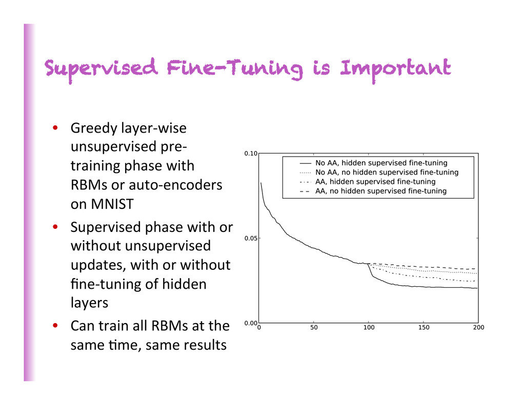
122. Supervised Fine-Tuning is Important •  Greedy  layer-­‐wise   unsupervised  pre-­‐ training  phase  with   RBMs  or  auto-­‐encoders   on  MNIST   •  Supervised  phase  with  or   without  unsupervised   updates,  with  or  without   fine-­‐tuning  of  hidden   layers   •  Can  train  all  RBMs  at  the   same  8me,  same  results  
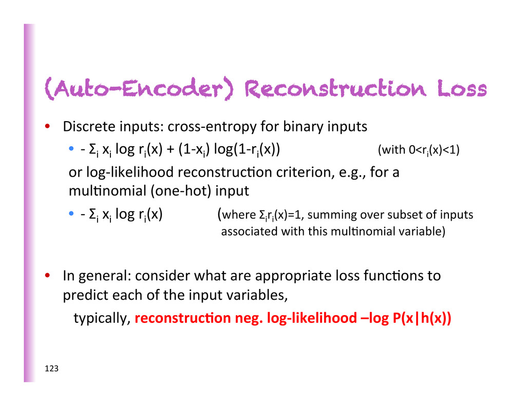
123. (Auto-Encoder) Reconstruction Loss •  Discrete  inputs:  cross-­‐entropy  for  binary  inputs   •  -­‐  Σi  xi  log  ri (x)  +  (1-­‐xi )  log(1-­‐ri (x))                                                      (with  0<ri (x)<1)   or  log-­‐likelihood  reconstruc8on  criterion,  e.g.,  for  a   mul8nomial  (one-­‐hot)  input   •  -­‐  Σi  xi  log  ri (x)                              (where  Σi ri (x)=1,  summing  over  subset  of  inputs                                  associated  with  this  mul8nomial  variable)     •  In  general:  consider  what  are  appropriate  loss  func8ons  to   predict  each  of  the  input  variables,                    typically,  reconstruc0on  neg.  log-­‐likelihood  –log  P(x|h(x))   123  
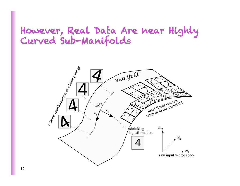
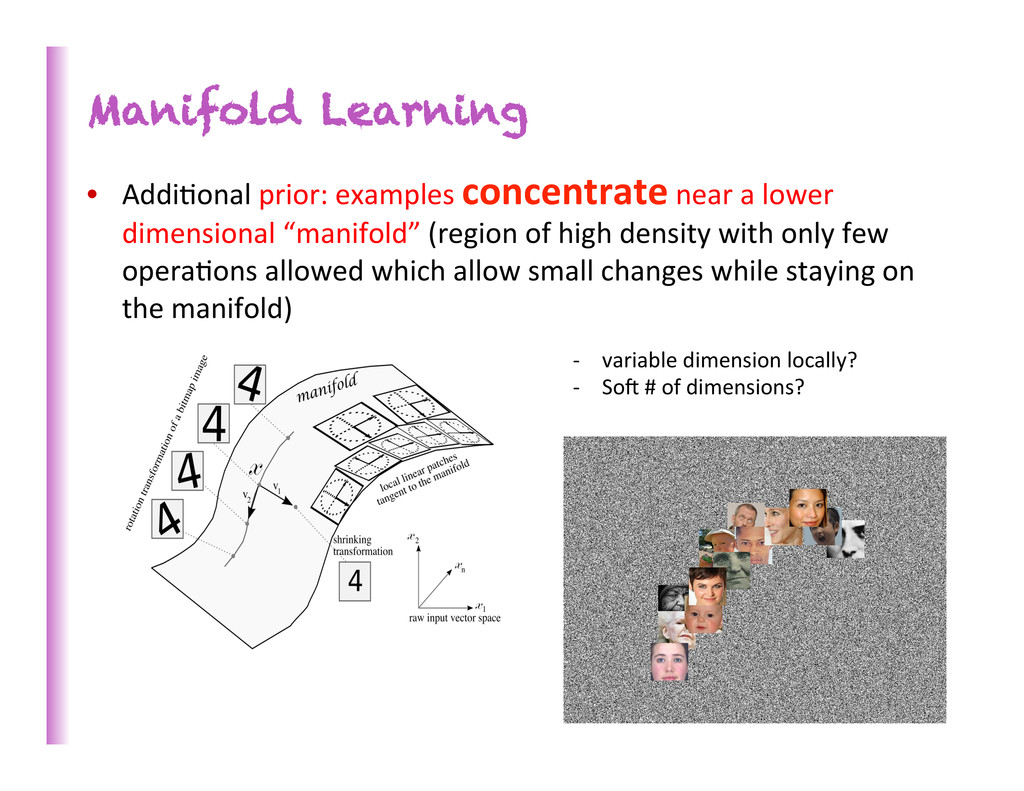
124. 124   Manifold Learning •  Addi8onal  prior:  examples  concentrate  near  a  lower   dimensional  “manifold”  (region  of  high  density  with  only  few   opera8ons  allowed  which  allow  small  changes  while  staying  on   the  manifold)   -­‐  variable  dimension  locally?   -­‐  SoZ  #  of  dimensions?  
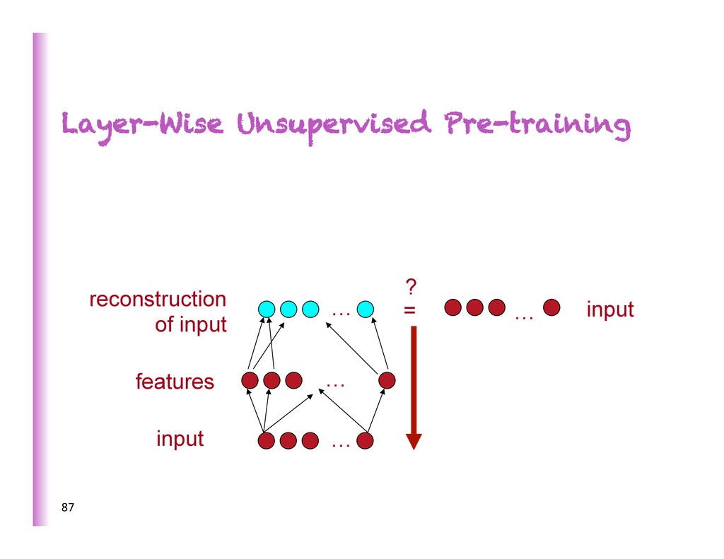
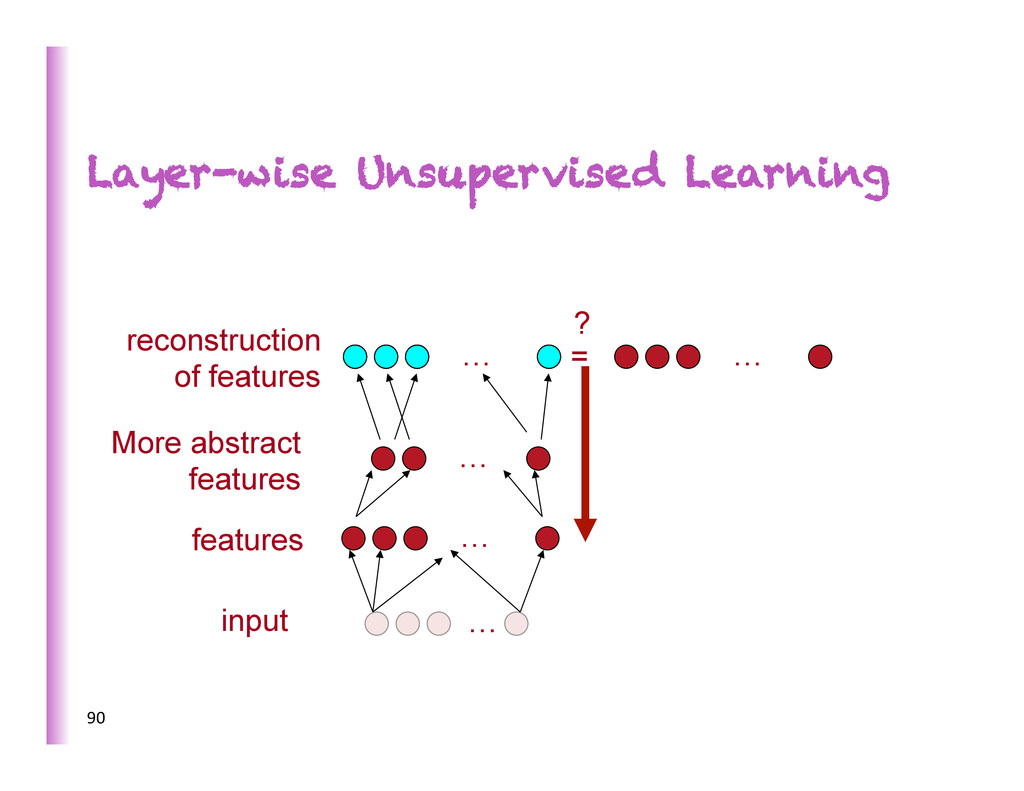
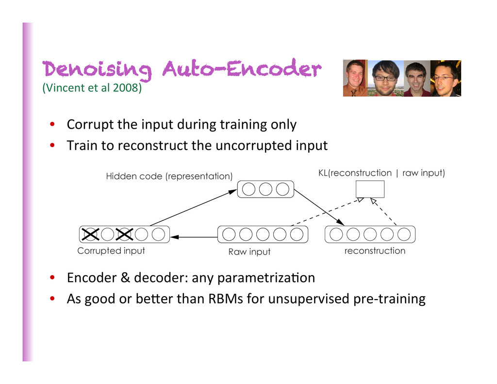
125. Denoising Auto-Encoder (Vincent  et  al  2008)   •  Corrupt  the  input  during  training  only   •  Train  to  reconstruct  the  uncorrupted  input   KL(reconstruction | raw input) Hidden code (representation) Corrupted input Raw input reconstruction •  Encoder  &  decoder:  any  parametriza8on   •  As  good  or  beber  than  RBMs  for  unsupervised  pre-­‐training  
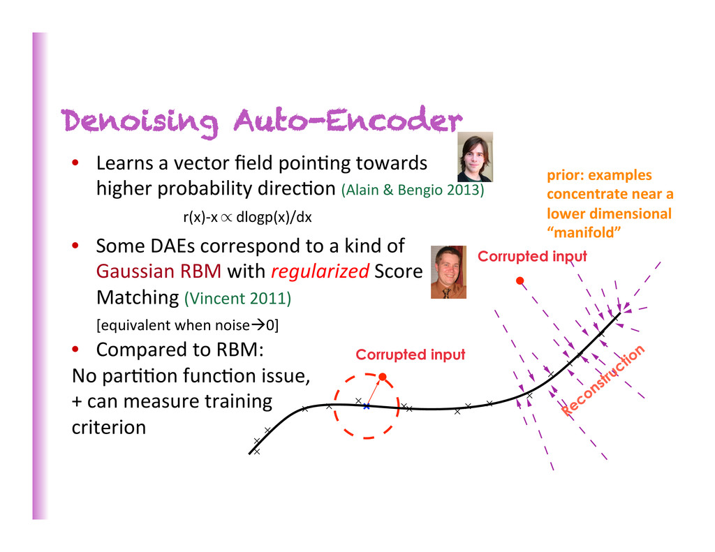
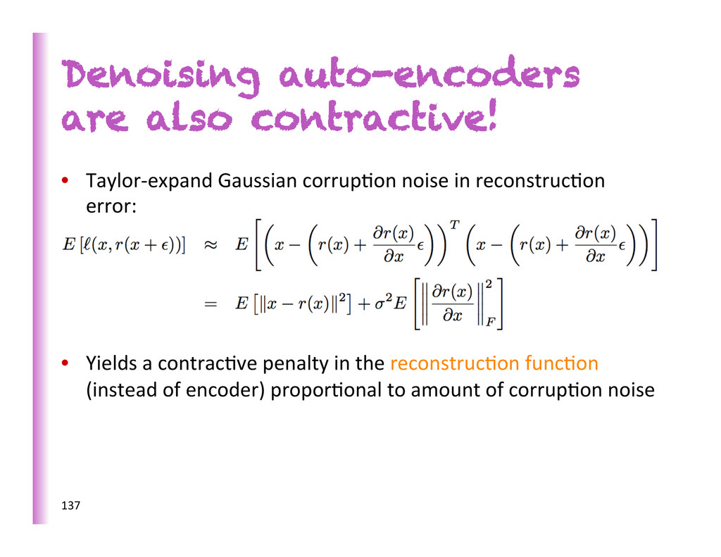
126. Denoising Auto-Encoder •  Learns  a  vector  field  poin8ng  towards   higher  probability  direc8on  (Alain  &  Bengio  2013)   •  Some  DAEs  correspond  to  a  kind  of   Gaussian  RBM  with  regularized  Score   Matching  (Vincent  2011)            [equivalent  when  noiseà0]   •  Compared  to  RBM:   No  par88on  func8on  issue,                                           +  can  measure  training                 criterion   Corrupted input Corrupted input prior:  examples   concentrate  near  a   lower  dimensional   “manifold”     r(x)-­‐x          dlogp(x)/dx   /
127. Stacked Denoising Auto-Encoders Infinite MNIST Note  how   advantage  of   beber   ini8aliza8on   does  not  vanish   like  other   regularizers  as   #exemplesà∞  
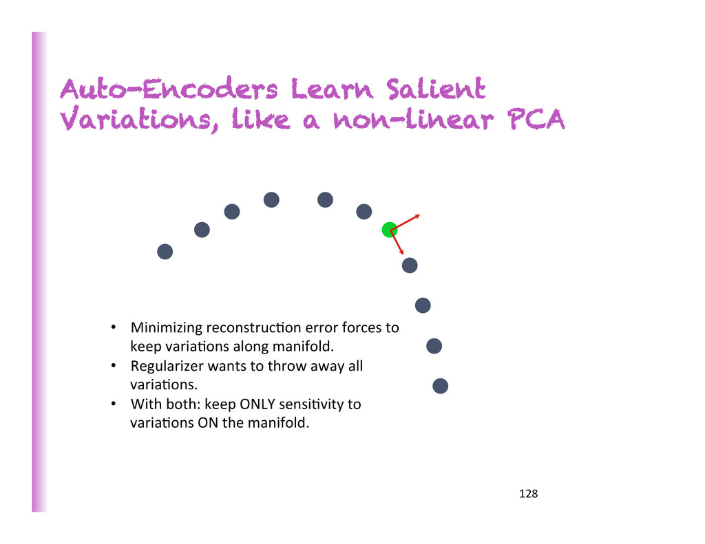
128. 128   Auto-Encoders Learn Salient Variations, like a non-linear PCA •  Minimizing  reconstruc8on  error  forces  to   keep  varia8ons  along  manifold.   •  Regularizer  wants  to  throw  away  all   varia8ons.   •  With  both:  keep  ONLY  sensi8vity  to   varia8ons  ON  the  manifold.  
129. Regularized Auto-Encoders Learn a Vector Field or a Markov Chain Transition Distribution •  (Bengio,  Vincent  &  Courville,  TPAMI  2013)  review  paper   •  (Alain  &  Bengio  ICLR  2013;  Bengio  et  al,  arxiv  2013)   129  
130. Contractive Auto-Encoders wants  contrac8on  in  all   direc8ons   cannot  afford  contrac8on  in   manifold  direc8ons   (Rifai,  Vincent,  Muller,  Glorot,  Bengio  ICML  2011;  Rifai,  Mesnil,   Vincent,  Bengio,  Dauphin,  Glorot  ECML  2011;  Rifai,  Dauphin,   Vincent,  Bengio,  Muller  NIPS  2011)   Training  criterion:     If  hj =sigmoid(bj +Wj  x)     (dhj (x)/dxi )2  =    hj 2(1-­‐hj )2Wji 2  
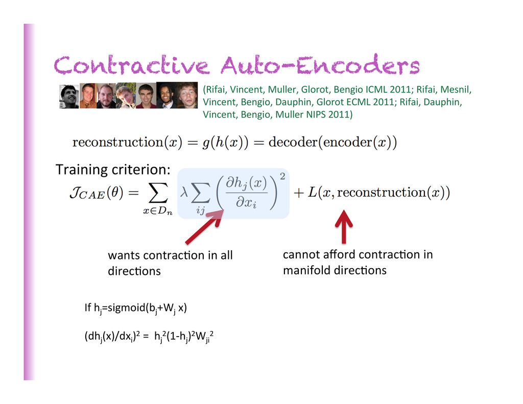
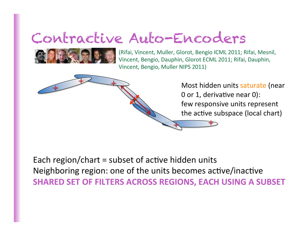
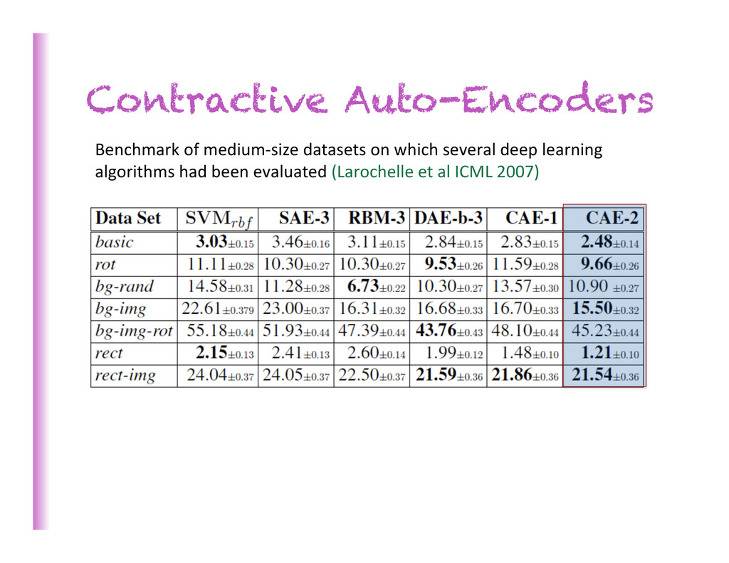
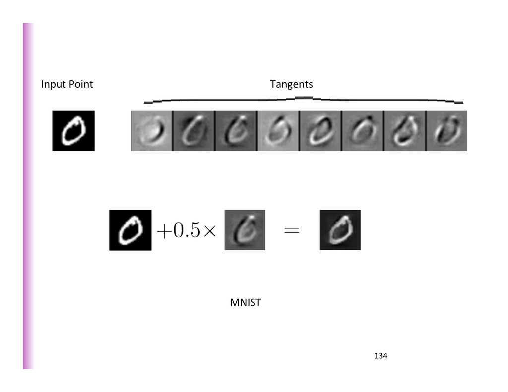
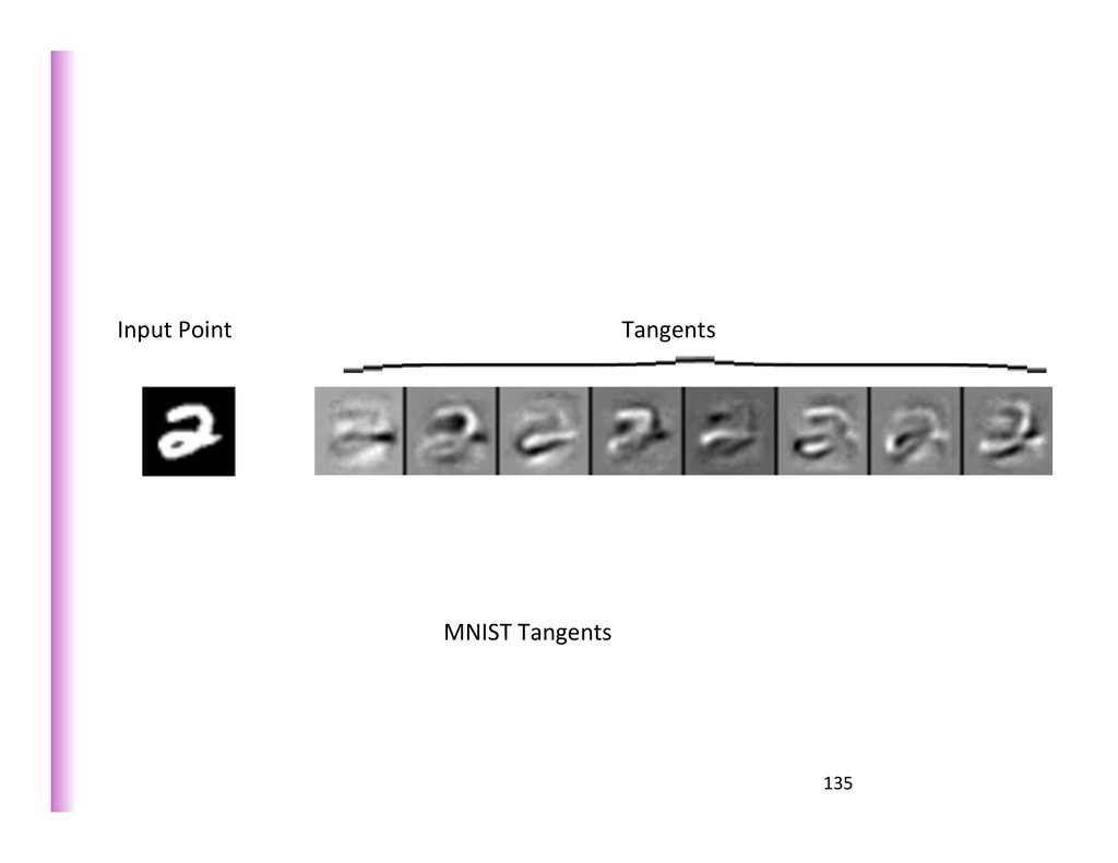
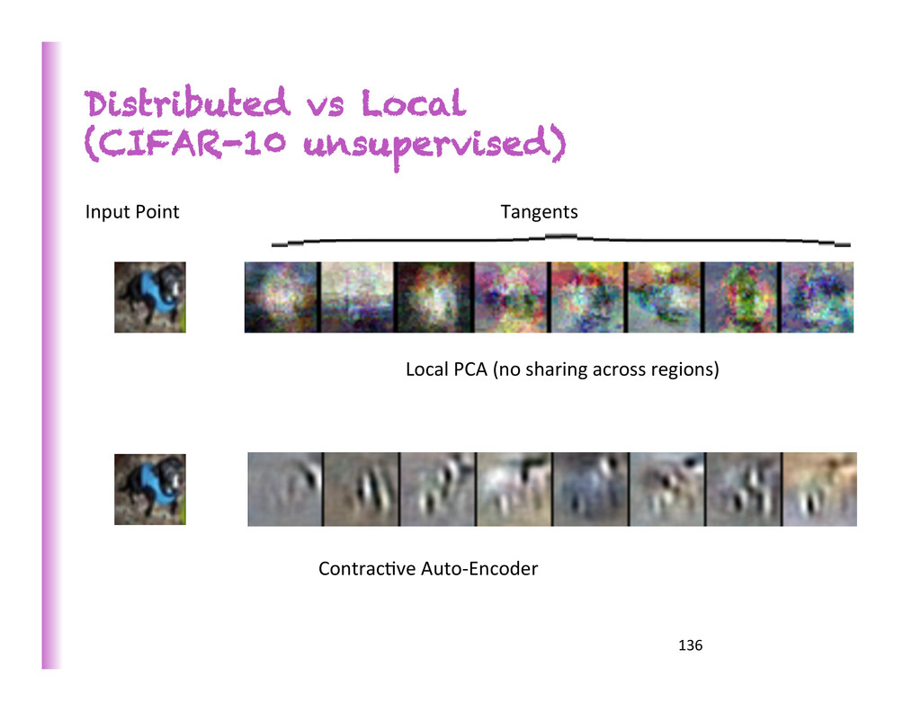
131. Most  hidden  units  saturate  (near   0  or  1,  deriva8ve  near  0):   few  responsive  units  represent   the  ac8ve  subspace  (local  chart)   Contractive Auto-Encoders (Rifai,  Vincent,  Muller,  Glorot,  Bengio  ICML  2011;  Rifai,  Mesnil,   Vincent,  Bengio,  Dauphin,  Glorot  ECML  2011;  Rifai,  Dauphin,   Vincent,  Bengio,  Muller  NIPS  2011)   Each  region/chart  =  subset  of  ac8ve  hidden  units   Neighboring  region:  one  of  the  units  becomes  ac8ve/inac8ve   SHARED  SET  OF  FILTERS  ACROSS  REGIONS,  EACH  USING  A  SUBSET  
132. 132   Jacobian’s  spectrum  is  peaked  =   local  low-­‐dimensional   representa8on  /  relevant  factors   Inac8ve  hidden  unit  =  0  singular  value  
133. Contractive Auto-Encoders Benchmark  of  medium-­‐size  datasets  on  which  several  deep  learning   algorithms  had  been  evaluated  (Larochelle  et  al  ICML  2007)  
134. 134   MNIST   Input  Point   Tangents  
135. 135   MNIST  Tangents   Input  Point   Tangents  
136. 136   Local  PCA  (no  sharing  across  regions)   Input  Point   Tangents   Contrac8ve  Auto-­‐Encoder   Distributed vs Local (CIFAR-10 unsupervised)
137. Denoising auto-encoders are also contractive! •  Taylor-­‐expand  Gaussian  corrup8on  noise  in  reconstruc8on   error:   •  Yields  a  contrac8ve  penalty  in  the  reconstruc8on  func8on   (instead  of  encoder)  propor8onal  to  amount  of  corrup8on  noise   137  
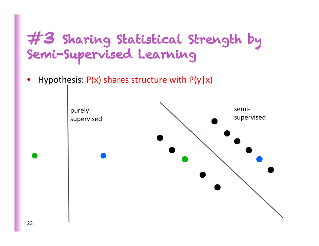
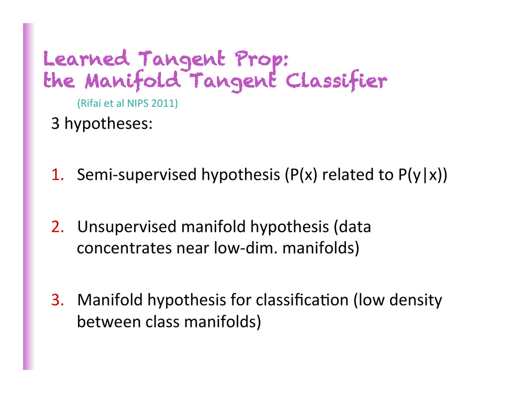
138. Learned Tangent Prop: the Manifold Tangent Classifier 3  hypotheses:     1.  Semi-­‐supervised  hypothesis  (P(x)  related  to  P(y|x))     2.  Unsupervised  manifold  hypothesis  (data   concentrates  near  low-­‐dim.  manifolds)   3.  Manifold  hypothesis  for  classifica8on  (low  density   between  class  manifolds)   (Rifai  et  al  NIPS  2011)  
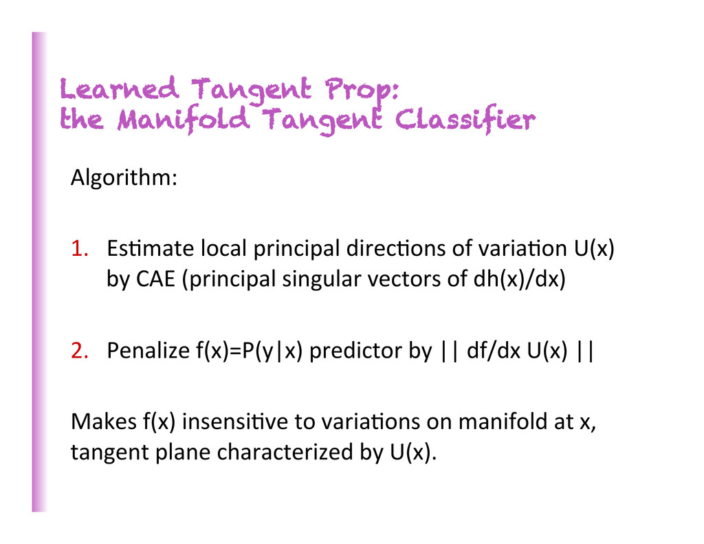
139. Learned Tangent Prop: the Manifold Tangent Classifier Algorithm:     1.  Es8mate  local  principal  direc8ons  of  varia8on  U(x)   by  CAE  (principal  singular  vectors  of  dh(x)/dx)   2.  Penalize  f(x)=P(y|x)  predictor  by  ||  df/dx  U(x)  ||   Makes  f(x)  insensi8ve  to  varia8ons  on  manifold  at  x,   tangent  plane  characterized  by  U(x).  
140. Manifold Tangent Classifier Results •  Leading  singular  vectors  on  MNIST,  CIFAR-­‐10,  RCV1:   •  Knowledge-­‐free  MNIST:  0.81%  error     •  Semi-­‐sup.       •  Forest  (500k  examples)    
141. Inference and Explaining Away •  Easy  inference  in  RBMs  and  regularized  Auto-­‐Encoders   •  But  no  explaining  away  (compe88on  between  causes)   •  (Coates  et  al  2011):  even  when  training  filters  as  RBMs  it  helps   to  perform  addi8onal  explaining  away  (e.g.  plug  them  into  a   Sparse  Coding  inference),  to  obtain  beber-­‐classifying  features   •  RBMs  would  need  lateral  connec8ons  to  achieve  similar  effect   •  Auto-­‐Encoders  would  need  to  have  lateral  recurrent   connec8ons  or  deep  recurrent  structure   141  
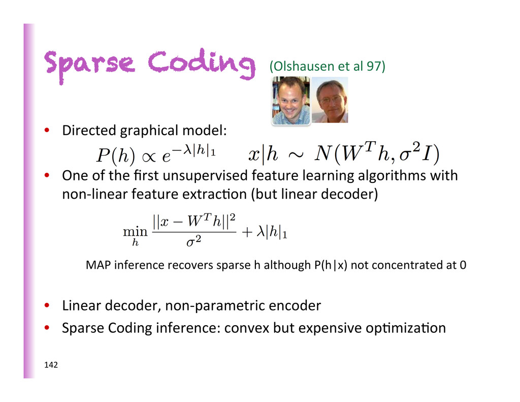
142. Sparse Coding (Olshausen  et  al  97)   •  Directed  graphical  model:     •  One  of  the  first  unsupervised  feature  learning  algorithms  with   non-­‐linear  feature  extrac8on  (but  linear  decoder)         MAP  inference  recovers  sparse  h  although  P(h|x)  not  concentrated  at  0     •  Linear  decoder,  non-­‐parametric  encoder   •  Sparse  Coding  inference:  convex  but  expensive  op8miza8on     142  
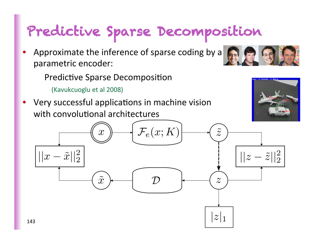
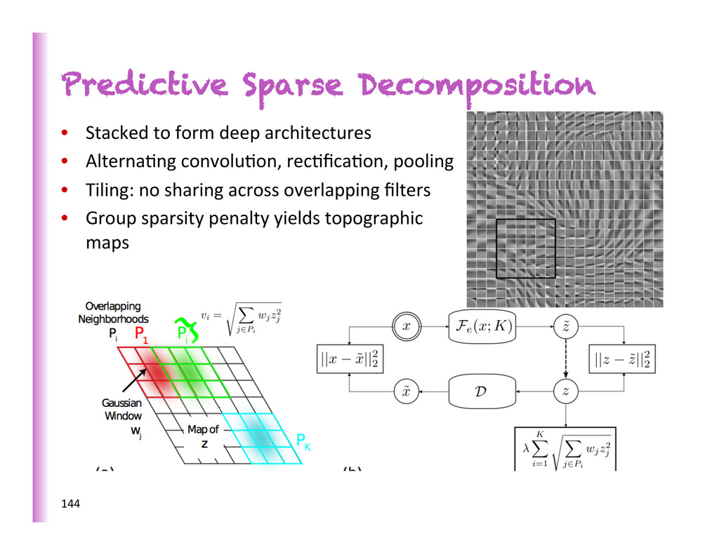
143. Predictive Sparse Decomposition •  Approximate  the  inference  of  sparse  coding  by  a   parametric  encoder:                      Predic8ve  Sparse  Decomposi8on                                      (Kavukcuoglu  et  al  2008)   •  Very  successful  applica8ons  in  machine  vision   with  convolu8onal  architectures   143  
144. Predictive Sparse Decomposition •  Stacked  to  form  deep  architectures   •  Alterna8ng  convolu8on,  rec8fica8on,  pooling   •  Tiling:  no  sharing  across  overlapping  filters   •  Group  sparsity  penalty  yields  topographic   maps   144  
145. Deep Variants 145  
146. Level-Local Learning is Important •  Ini8alizing  each  layer  of  an  unsupervised  deep  Boltzmann   machine  helps  a  lot     •  Ini8alizing  each  layer  of  a  supervised  neural  network  as  an  RBM,   auto-­‐encoder,  denoising  auto-­‐encoder,  etc  can  help  a  lot   •  Helps  most  the  layers  further  away  from  the  target   •  Not  just  an  effect  of  the  unsupervised  prior   •  Jointly  training  all  the  levels  of  a  deep  architecture  is  difficult   because  of  the  increased  non-­‐linearity  /  non-­‐smoothness   •  Ini8alizing  using  a  level-­‐local  learning  algorithm  is  a  useful  trick       •  Providing  intermediate-­‐level  targets  can  help  tremendously   (Gulcehre  &  Bengio  ICLR  2013)  
147. Stack of RBMs / AEs à Deep MLP •  Encoder  or  P(h|v)  becomes  MLP  layer       147   x   h3   h2   h1   x   h3   h2   h1   h1   h2   W1   W2   W3   W1   W2   W3   y   ^  
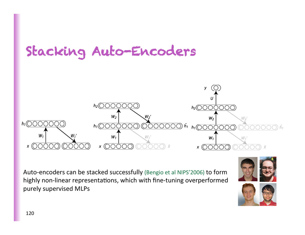
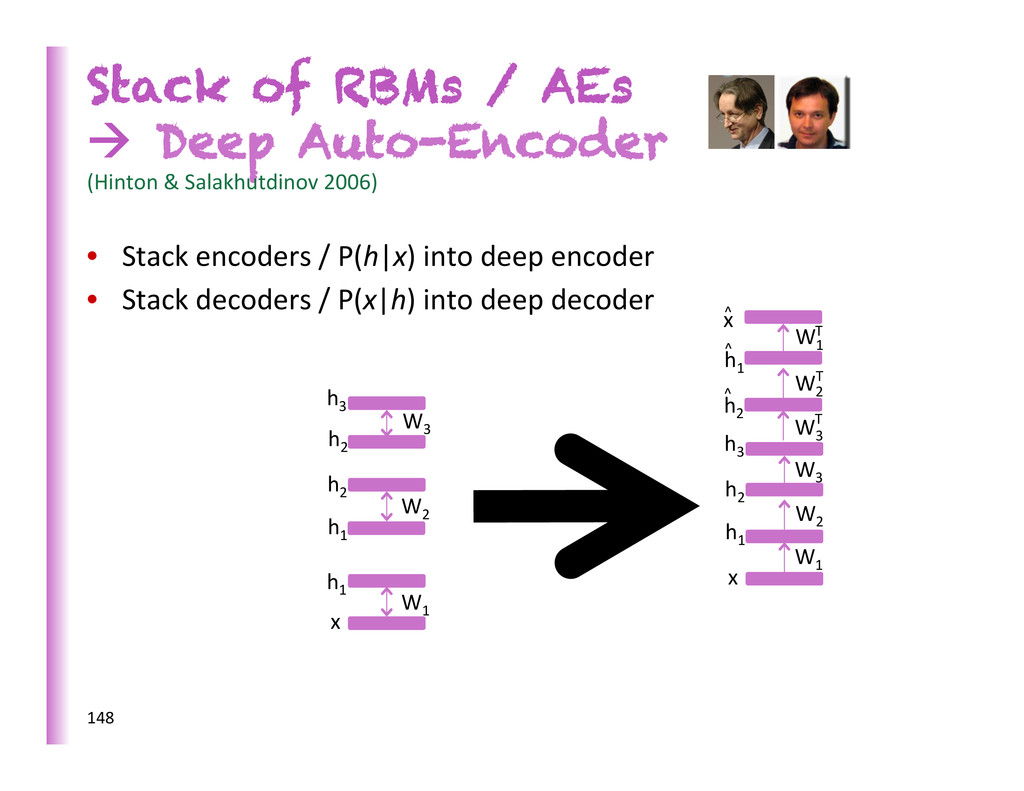
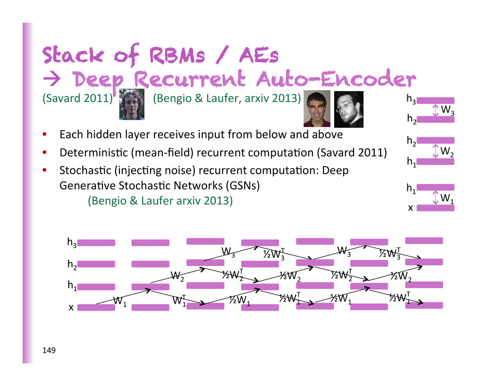
148. Stack of RBMs / AEs à Deep Auto-Encoder (Hinton  &  Salakhutdinov  2006)   •  Stack  encoders  /  P(h|x)  into  deep  encoder   •  Stack  decoders  /  P(x|h)  into  deep  decoder   148   x   h3   h2   h1   x   h3   h2   h1   h1   h2   x   h2   h1   ^   ^   ^   W1   W2   W3   W1   W1   T   W2   W2   T   W3   W3   T  
149. Stack of RBMs / AEs à Deep Recurrent Auto-Encoder (Savard  2011)                            (Bengio  &  Laufer,  arxiv  2013)   •  Each  hidden  layer  receives  input  from  below  and  above   •  Determinis8c  (mean-­‐field)  recurrent  computa8on  (Savard  2011)   •  Stochas8c  (injec8ng  noise)  recurrent  computa8on:  Deep   Genera8ve  Stochas8c  Networks  (GSNs)      (Bengio  &  Laufer  arxiv  2013)     149   x   h3   h2   h1   h1   h2   W1   W2   W3   x   h3   h2   h1   W1   ½W1   W1   T   ½W1   W2   ½W2   T   W3   ½W1   T   ½W1   T   ½W2   ½W2   T   ½W2   ½W3   T   W3   ½W3   T  
150. Stack of RBMs à Deep Belief Net (Hinton  et  al  2006)   •  Stack  lower  levels  RBMs’  P(x|h)  along  with  top-­‐level  RBM   •  P(x,  h1   ,  h2   ,  h3 )  =  P(h2   ,  h3 )  P(h1 |h2 )  P(x  |  h1 )   •  Sample:  Gibbs  on  top  RBM,  propagate  down   150   x   h3   h2   h1  
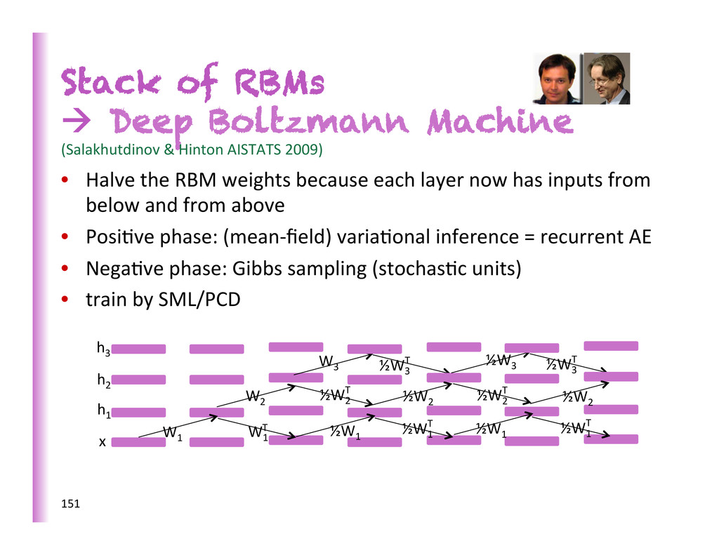
151. Stack of RBMs à Deep Boltzmann Machine (Salakhutdinov  &  Hinton  AISTATS  2009)   •  Halve  the  RBM  weights  because  each  layer  now  has  inputs  from   below  and  from  above   •  Posi8ve  phase:  (mean-­‐field)  varia8onal  inference  =  recurrent  AE   •  Nega8ve  phase:  Gibbs  sampling  (stochas8c  units)   •  train  by  SML/PCD   151   x   h3   h2   h1   W1   ½W1   W1   T   ½W1   W2   ½W2   T   W3   ½W1   T   ½W1   T   ½W2   ½W2   T   ½W2   ½W3   T   ½W3   ½W3   T  
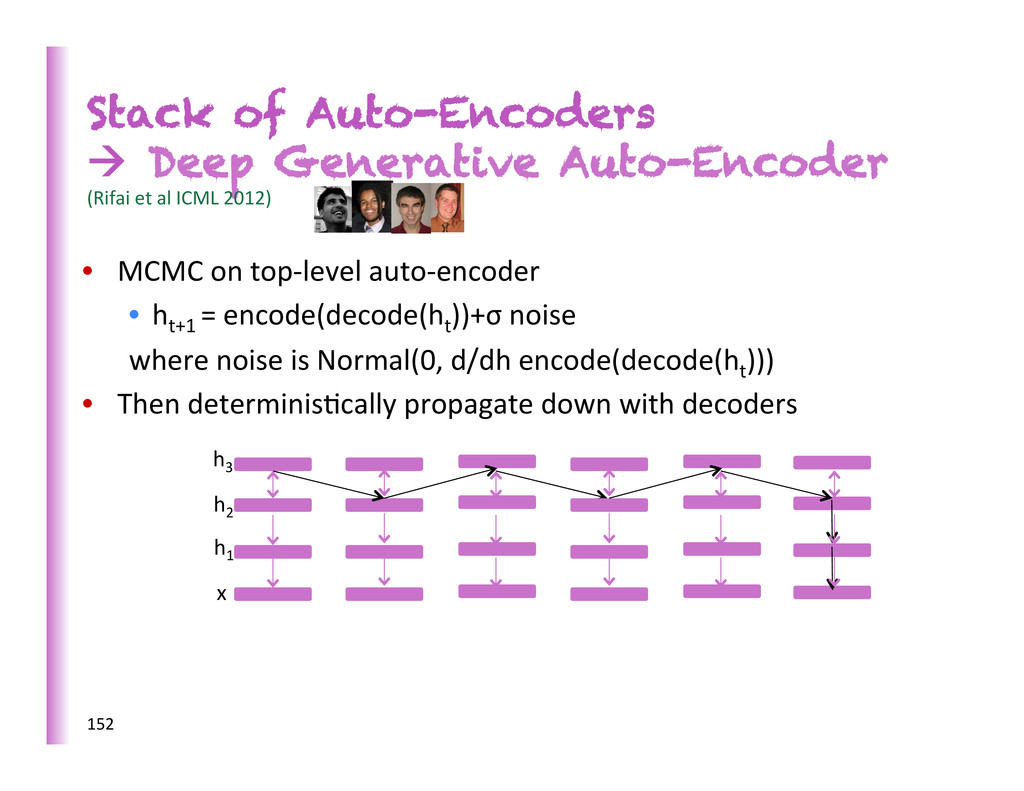
152. Stack of Auto-Encoders à Deep Generative Auto-Encoder (Rifai  et  al  ICML  2012)   •  MCMC  on  top-­‐level  auto-­‐encoder   •  ht+1   =  encode(decode(ht ))+σ  noise   where  noise  is  Normal(0,  d/dh  encode(decode(ht )))   •  Then  determinis8cally  propagate  down  with  decoders     152   x   h3   h2   h1  
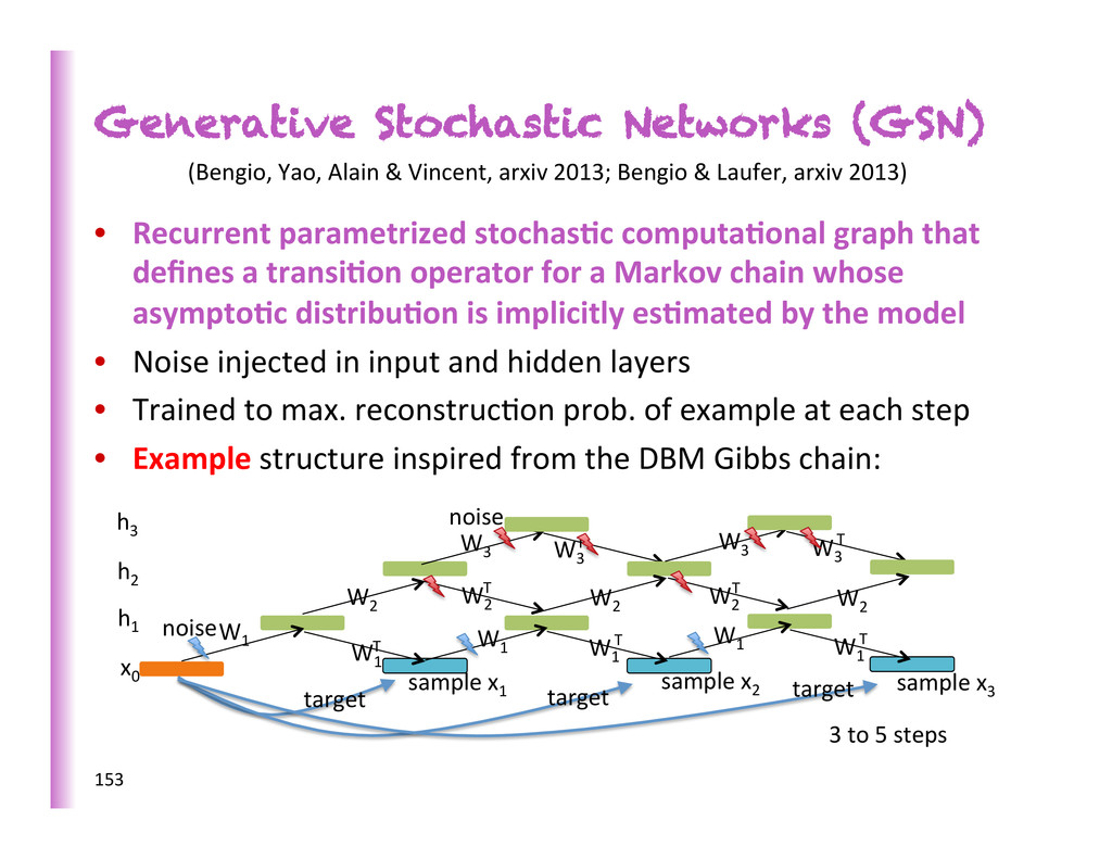
153. Generative Stochastic Networks (GSN) •  Recurrent  parametrized  stochas0c  computa0onal  graph  that   defines  a  transi0on  operator  for  a  Markov  chain  whose   asympto0c  distribu0on  is  implicitly  es0mated  by  the  model   •  Noise  injected  in  input  and  hidden  layers   •  Trained  to  max.  reconstruc8on  prob.  of  example  at  each  step   •  Example  structure  inspired  from  the  DBM  Gibbs  chain:   153   1" x 0" h 3" h 2" h 1" W 1" W 1" W 1" T" W 1" W 2" W 2" T" W 3" W 1" T" W 1" T" W 2" W 2" T" W 2" W 3" T" W 3" W 3" T" sample"x 1 " sample"x 2 " sample"x 3 " target" target" target" noise   noise   3  to  5  steps   (Bengio,  Yao,  Alain  &  Vincent,  arxiv  2013;  Bengio  &  Laufer,  arxiv  2013)  
154. Denoising Auto-Encoder Markov Chain •                   :  true  data-­‐genera8ng  distribu8on   •                             :  corrup8on  process   •                                 :  denoising  auto-­‐encoder  trained  with  n  examples   from                                                          ,    probabilis8cally  “inverts”  corrup8on   •           :  Markov  chain  over  X  alterna8ng                                                  ,       154   Xt   Xt   ~   Xt+1   ~   Xt+1   Xt+2   Xt+2   ~   corrupt   denoise  
155. Previous Theoretical Results on Probabilistic Interpretation of Auto- Encoders •  Con8nuous  X   •  Gaussian  corrup8on   •  Noise  σ  à  0   •  Squared  reconstruc8on  error  ||r(X+noise)-­‐X||2      (r(X)-­‐X)/σ2    es8mates  the  score  d  log  p(X)  /  dX   155   (Vincent  2011,  Alain  &  Bengio  2013)  
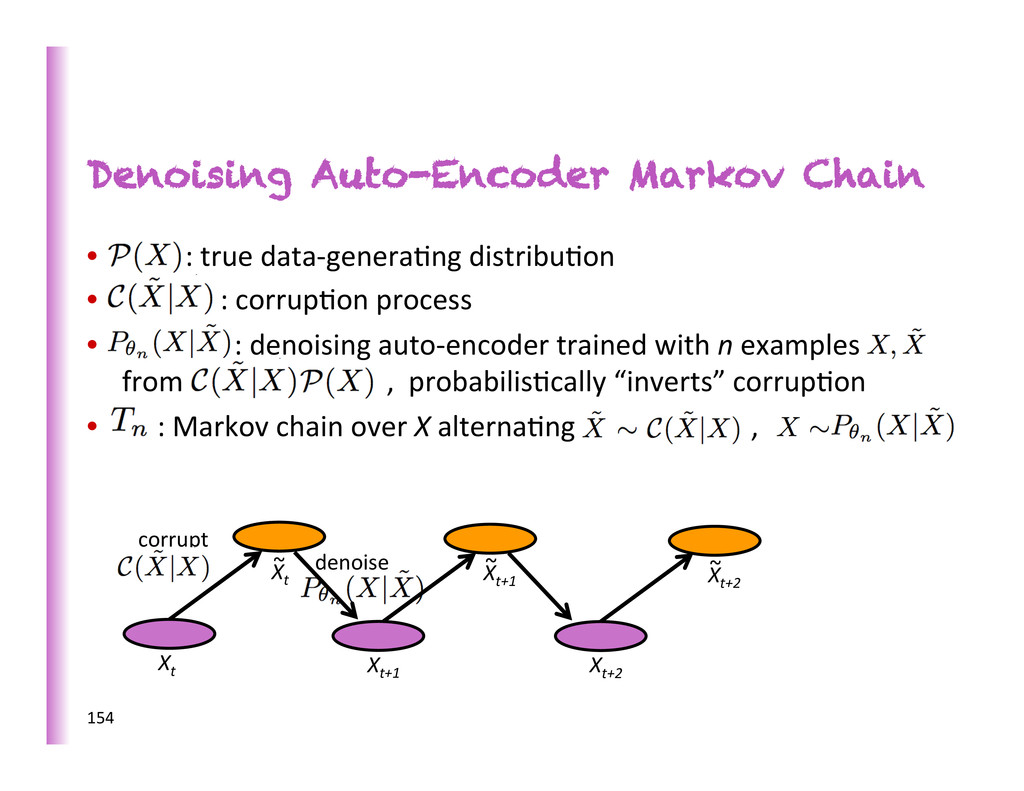
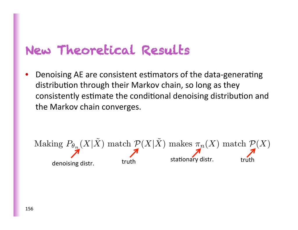
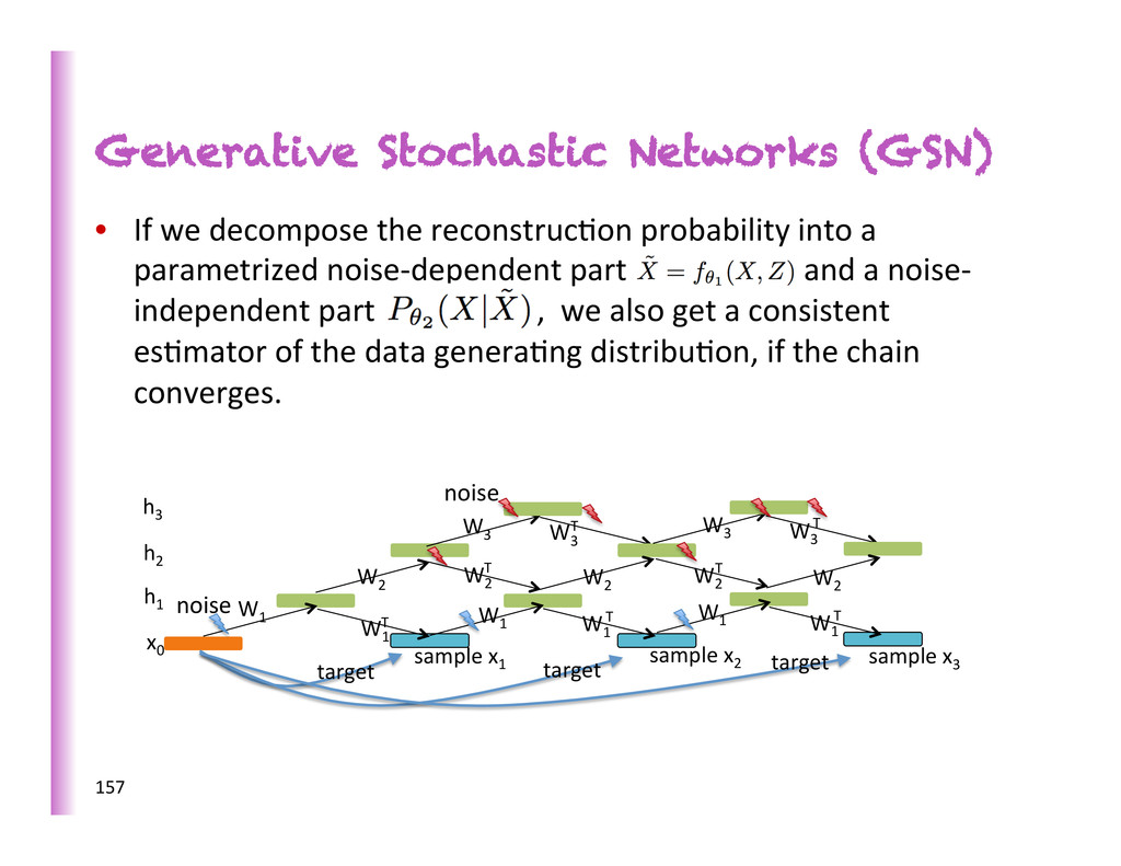
156. New Theoretical Results 156   •  Denoising  AE  are  consistent  es8mators  of  the  data-­‐genera8ng   distribu8on  through  their  Markov  chain,  so  long  as  they   consistently  es8mate  the  condi8onal  denoising  distribu8on  and   the  Markov  chain  converges.   Making P✓n (X| ˜ X) match P(X| ˜ X) makes ⇡n(X) match P(X) truth   denoising  distr.   sta8onary  distr.   truth  
157. Generative Stochastic Networks (GSN) •  If  we  decompose  the  reconstruc8on  probability  into  a   parametrized  noise-­‐dependent  part                                              and  a  noise-­‐ independent  part                                          ,    we  also  get  a  consistent   es8mator  of  the  data  genera8ng  distribu8on,  if  the  chain   converges.   157   1" x 0" h 3" h 2" h 1" W 1" W 1" W 1" T" W 1" W 2" W 2" T" W 3" W 1" T" W 1" T" W 2" W 2" T" W 2" W 3" T" W 3" W 3" T" sample"x 1 " sample"x 2 " sample"x 3 " target" target" target" noise   noise  
158. GSN Experiments: validating the theorem in a continuous non- parametric setting •  Con8nuous  data,         X  in  R10,  Gaussian   corrup8on   •  Reconstruc8on   distribu8on  =   Parzen  (mixture  of   Gaussians)   es8mator   •  5000  training   examples,  5000   samples   •  Visualize  a  pair  of   dimensions   158  
159. GSN Experiments: validating the theorem in a continuous non-parametric setting 159  
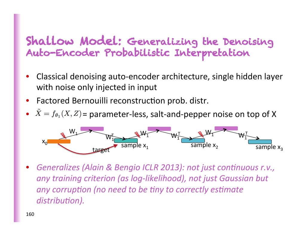
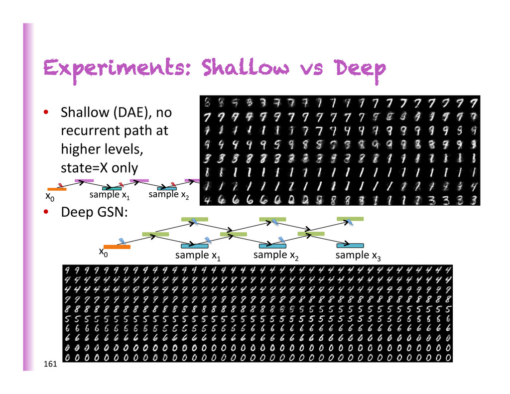
160. Shallow Model: Generalizing the Denoising Auto-Encoder Probabilistic Interpretation •  Classical  denoising  auto-­‐encoder  architecture,  single  hidden  layer   with  noise  only  injected  in  input   •  Factored  Bernouilli  reconstruc8on  prob.  distr.   •                                             =  parameter-­‐less,  salt-­‐and-­‐pepper  noise  on  top  of  X   •  Generalizes  (Alain  &  Bengio  ICLR  2013):  not  just  conKnuous  r.v.,   any  training  criterion  (as  log-­‐likelihood),  not  just  Gaussian  but   any  corrupKon  (no  need  to  be  Kny  to  correctly  esKmate   distribuKon).   160   x0   W1   W1   W1   T   W1   W1   T   W1   T   sample  x1   sample  x2   target   sample  x3  
161. Experiments: Shallow vs Deep •  Shallow  (DAE),  no   recurrent  path  at   higher  levels,   state=X  only   •  Deep  GSN:   161   x0   sample  x1   sample  x2   x3   x0   sample  x1   sample  x2   sample  x3  
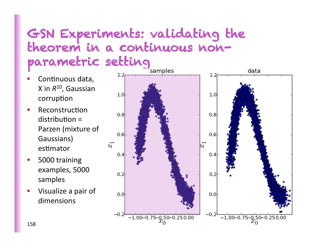
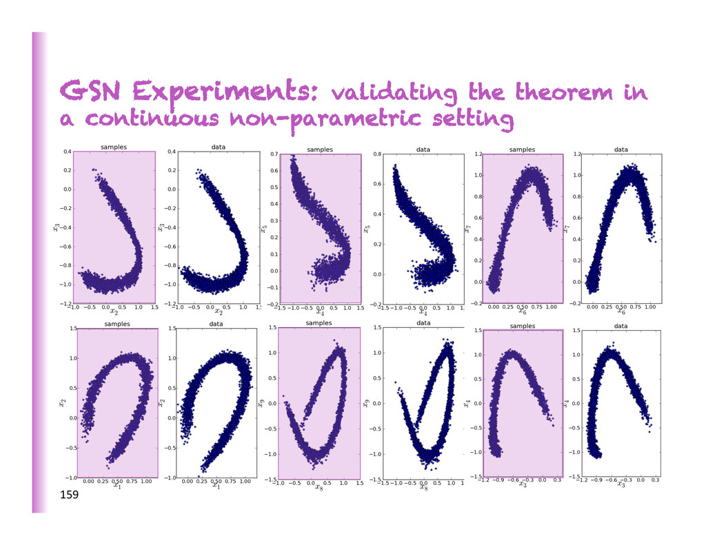
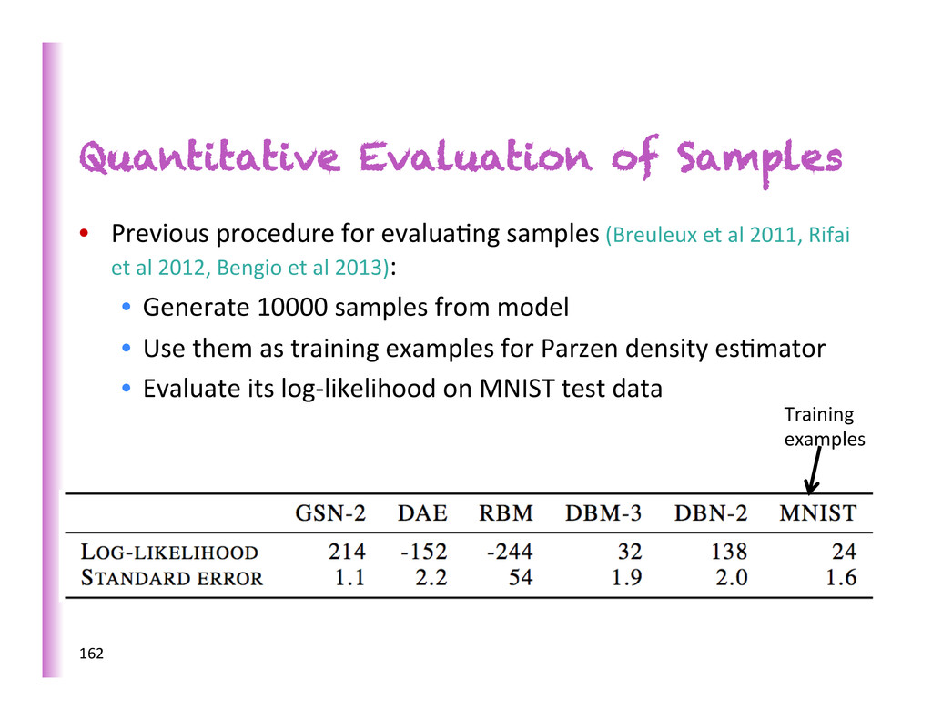
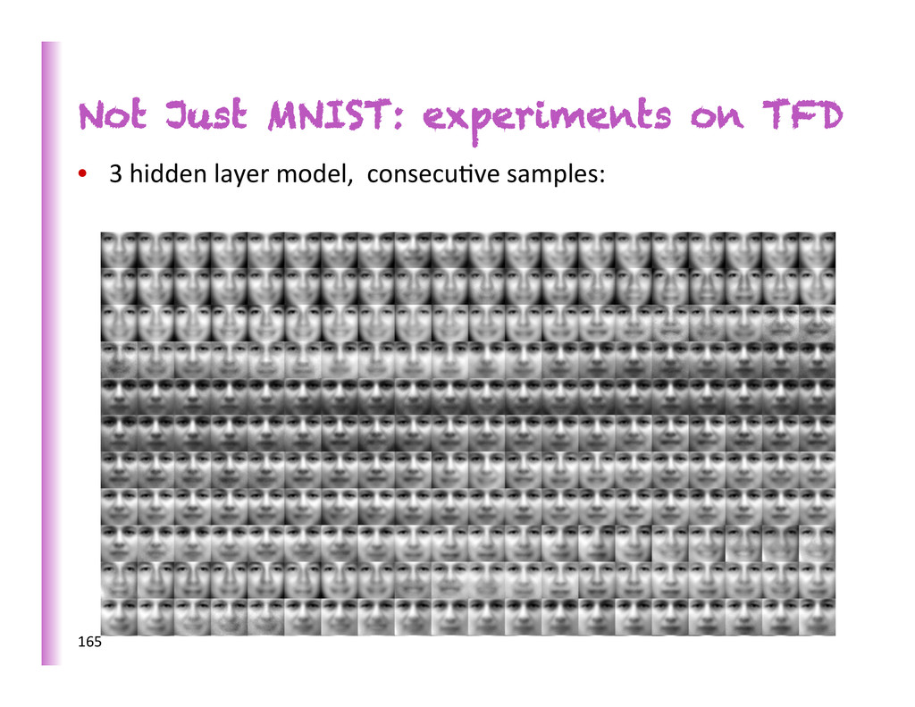
162. Quantitative Evaluation of Samples •  Previous  procedure  for  evalua8ng  samples  (Breuleux  et  al  2011,  Rifai   et  al  2012,  Bengio  et  al  2013):   •  Generate  10000  samples  from  model   •  Use  them  as  training  examples  for  Parzen  density  es8mator   •  Evaluate  its  log-­‐likelihood  on  MNIST  test  data   162   Training   examples  
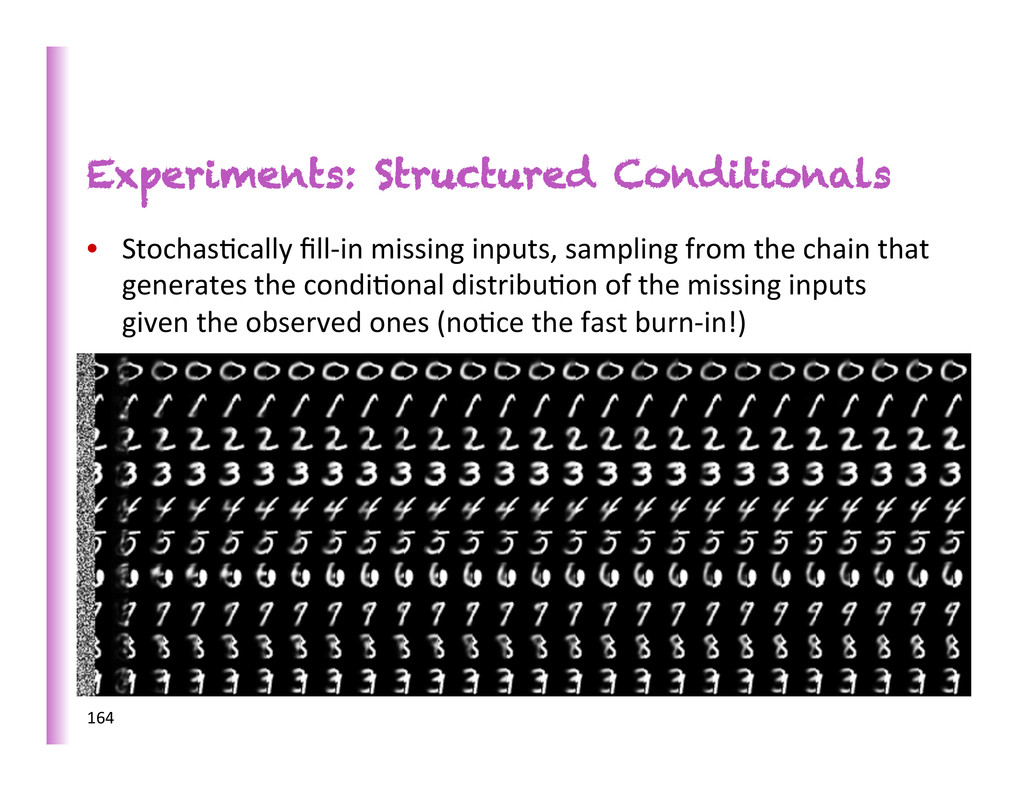
163. Question Answering, Missing Inputs and Structured Output •  Once  trained,  a  GSN  can  provably  sample  from  any  condi8onal   over  subsets  of  its  inputs,  so  long  as  we  use  the  condi8onal   associated  with  the  reconstruc8on  distribu8on  and  clamp  the   right-­‐hand  side  variables.   (Bengio  &  Laufer  arXiv  2013)   163  
164. Experiments: Structured Conditionals •  Stochas8cally  fill-­‐in  missing  inputs,  sampling  from  the  chain  that   generates  the  condi8onal  distribu8on  of  the  missing  inputs   given  the  observed  ones  (no8ce  the  fast  burn-­‐in!)   164  
165. Not Just MNIST: experiments on TFD •  3  hidden  layer  model,    consecu8ve  samples:   165  
166. Practical Considerations Part  3   166  
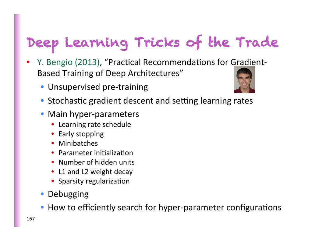
167. Deep Learning Tricks of the Trade •  Y.  Bengio  (2013),  “Prac8cal  Recommenda8ons  for  Gradient-­‐ Based  Training  of  Deep  Architectures”     •  Unsupervised  pre-­‐training   •  Stochas8c  gradient  descent  and  se€ng  learning  rates   •  Main  hyper-­‐parameters   •  Learning  rate  schedule   •  Early  stopping   •  Minibatches   •  Parameter  ini8aliza8on   •  Number  of  hidden  units   •  L1  and  L2  weight  decay   •  Sparsity  regulariza8on   •  Debugging   •  How  to  efficiently  search  for  hyper-­‐parameter  configura8ons   167  
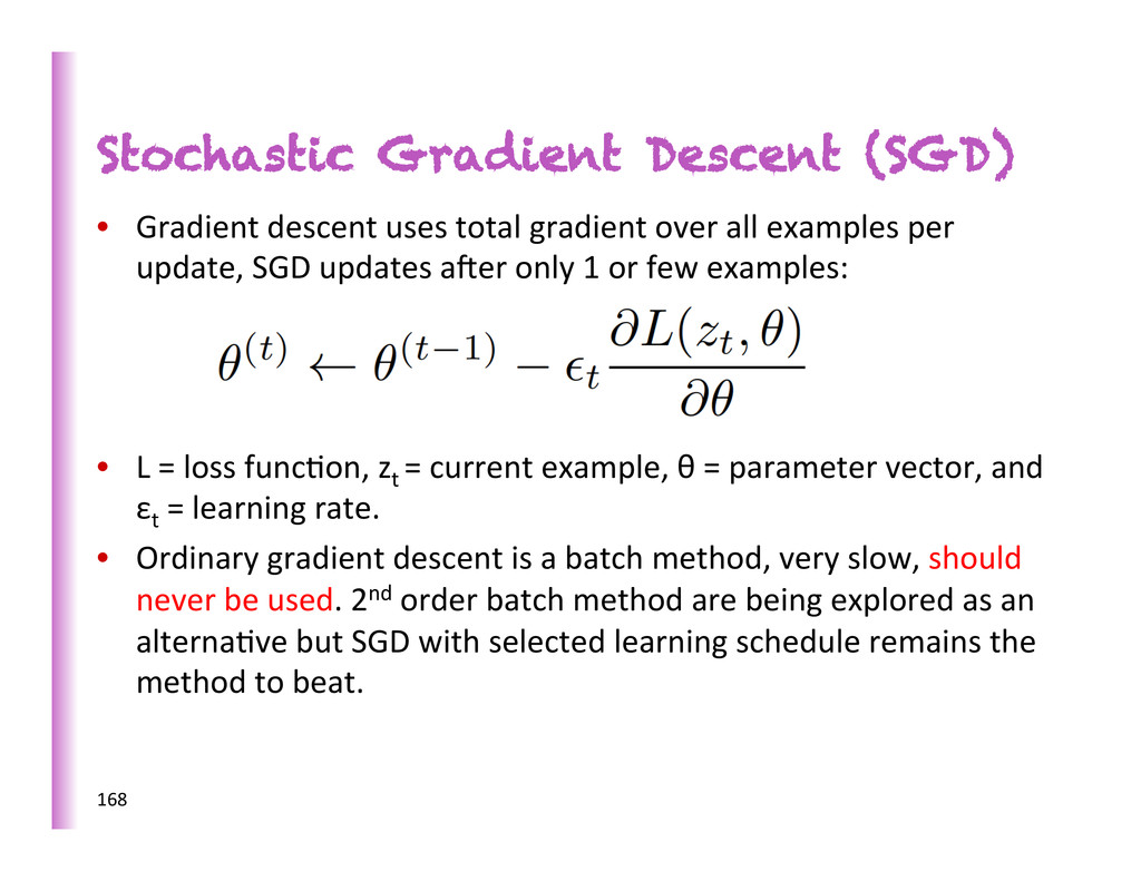
168. •  Gradient  descent  uses  total  gradient  over  all  examples  per   update,  SGD  updates  aZer  only  1  or  few  examples:   •  L  =  loss  func8on,  zt   =  current  example,  θ  =  parameter  vector,  and   εt  =  learning  rate.   •  Ordinary  gradient  descent  is  a  batch  method,  very  slow,  should   never  be  used.  2nd  order  batch  method  are  being  explored  as  an   alterna8ve  but  SGD  with  selected  learning  schedule  remains  the   method  to  beat.   Stochastic Gradient Descent (SGD) 168  
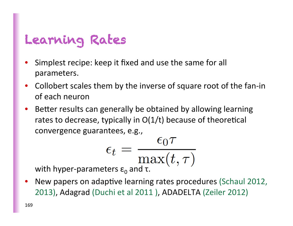
169. Learning Rates •  Simplest  recipe:  keep  it  fixed  and  use  the  same  for  all   parameters.   •  Collobert  scales  them  by  the  inverse  of  square  root  of  the  fan-­‐in   of  each  neuron   •  Beber  results  can  generally  be  obtained  by  allowing  learning   rates  to  decrease,  typically  in  O(1/t)  because  of  theore8cal   convergence  guarantees,  e.g.,              with  hyper-­‐parameters  ε0  and  τ.   •  New  papers  on  adap8ve  learning  rates  procedures  (Schaul  2012,   2013),  Adagrad  (Duchi  et  al  2011  ),  ADADELTA  (Zeiler  2012)   169  
170. Early Stopping •  Beau8ful  FREE  LUNCH  (no  need  to  launch  many  different   training  runs  for  each  value  of  hyper-­‐parameter  for  #itera8ons)   •  Monitor  valida8on  error  during  training  (aZer  visi8ng  #  of   training  examples  =  a  mul8ple  of  valida8on  set  size)   •  Keep  track  of  parameters  with  best  valida8on  error  and  report   them  at  the  end   •  If  error  does  not  improve  enough  (with  some  pa8ence),  stop.   170  
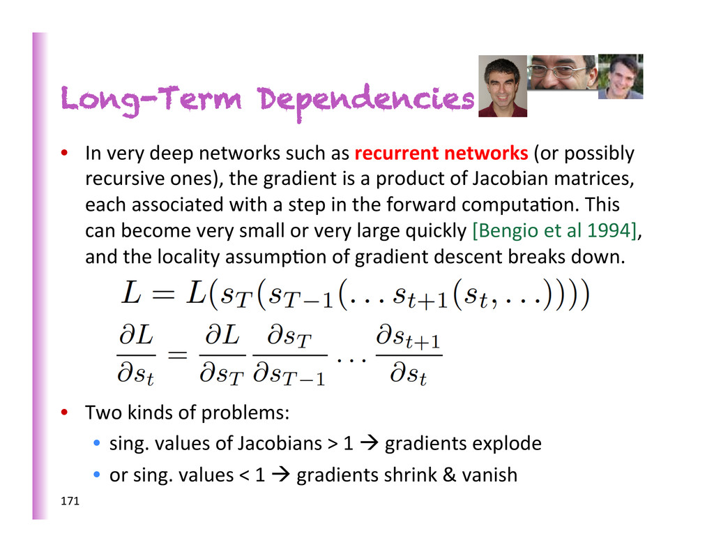
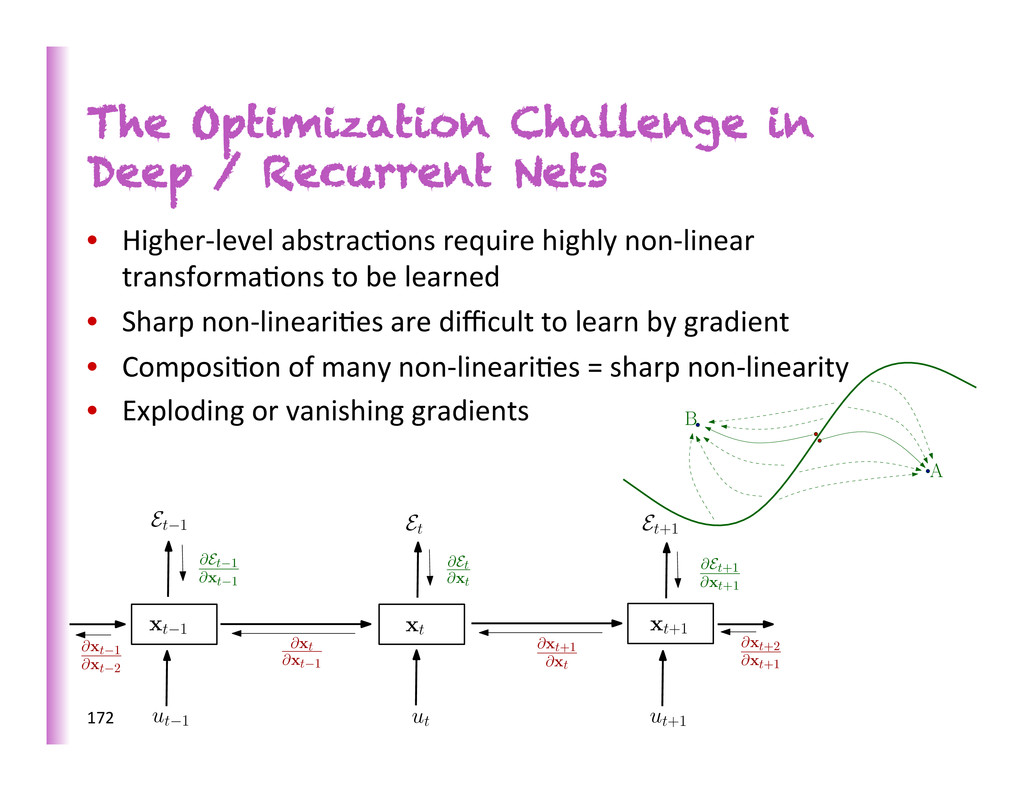
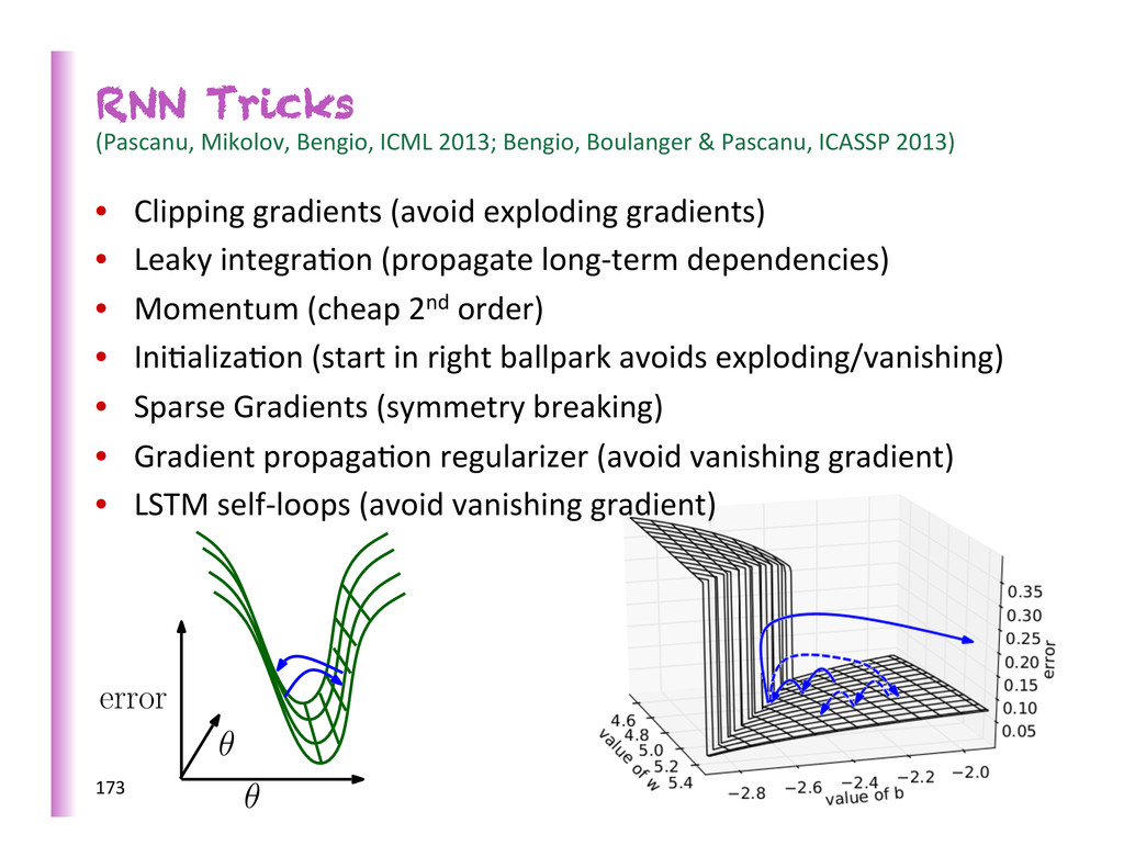
171. Long-Term Dependencies •  In  very  deep  networks  such  as  recurrent  networks  (or  possibly   recursive  ones),  the  gradient  is  a  product  of  Jacobian  matrices,   each  associated  with  a  step  in  the  forward  computa8on.  This   can  become  very  small  or  very  large  quickly  [Bengio  et  al  1994],   and  the  locality  assump8on  of  gradient  descent  breaks  down.     •  Two  kinds  of  problems:     •  sing.  values  of  Jacobians  >  1  à  gradients  explode   •  or  sing.  values  <  1  à  gradients  shrink  &  vanish     171  
172. The Optimization Challenge in Deep / Recurrent Nets •  Higher-­‐level  abstrac8ons  require  highly  non-­‐linear   transforma8ons  to  be  learned   •  Sharp  non-­‐lineari8es  are  difficult  to  learn  by  gradient   •  Composi8on  of  many  non-­‐lineari8es  =  sharp  non-­‐linearity   •  Exploding  or  vanishing  gradients   172   @Et+1 @ xt+1 Et+1 Et Et 1 xt+1 xt xt 1 ut 1 ut ut+1 @Et @ xt @Et 1 @ xt 1 @ xt+2 @ xt+1 @ xt+1 @ xt @ xt @ xt 1 @ xt 1 @ xt 2 A B
173. RNN Tricks (Pascanu,  Mikolov,  Bengio,  ICML  2013;  Bengio,  Boulanger  &  Pascanu,  ICASSP  2013)   •  Clipping  gradients  (avoid  exploding  gradients)   •  Leaky  integra8on  (propagate  long-­‐term  dependencies)   •  Momentum  (cheap  2nd  order)   •  Ini8aliza8on  (start  in  right  ballpark  avoids  exploding/vanishing)   •  Sparse  Gradients  (symmetry  breaking)   •  Gradient  propaga8on  regularizer  (avoid  vanishing  gradient)   •  LSTM  self-­‐loops  (avoid  vanishing  gradient)   173   error ✓ ✓
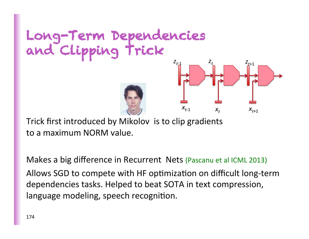
174. Long-Term Dependencies and Clipping Trick   Trick  first  introduced  by  Mikolov    is  to  clip  gradients   to  a  maximum  NORM  value.       Makes  a  big  difference  in  Recurrent    Nets  (Pascanu  et  al  ICML  2013)   Allows  SGD  to  compete  with  HF  op8miza8on  on  difficult  long-­‐term   dependencies  tasks.  Helped  to  beat  SOTA  in  text  compression,   language  modeling,  speech  recogni8on.     174   xt-­‐1   xt   xt+1   zt-­‐1   zt   zt+1  
175. Combining clipping to avoid gradient explosion and Jacobian regularizer to avoid gradient vanishing •  (Pascanu,  Mikolov  &  Bengio,  ICML  2013)   175   x h y
176. Normalized Initialization to Achieve Unity-Like Jacobian Assuming  f’(act=0)=1  
177. Normalized Initialization with Variance- Preserving Jacobians Shapeset 2x3 data Unsupervised pre-training: Automatically variance- preserving!
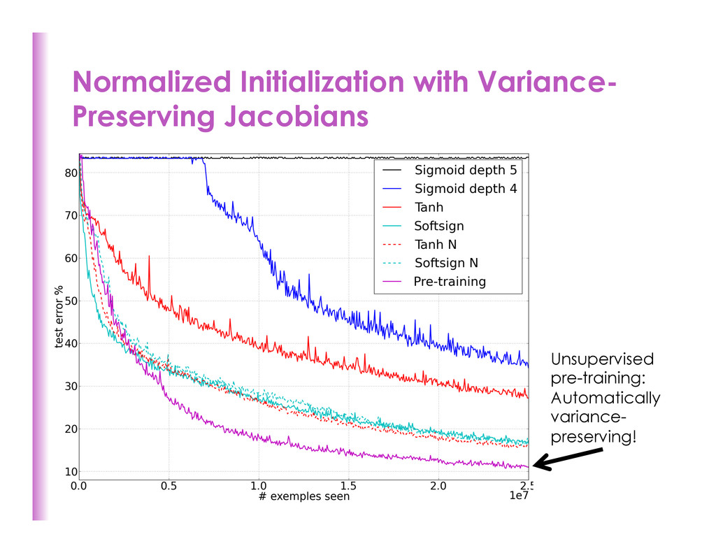
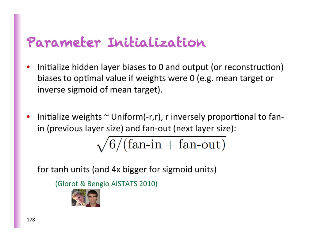
178. Parameter Initialization •  Ini8alize  hidden  layer  biases  to  0  and  output  (or  reconstruc8on)   biases  to  op8mal  value  if  weights  were  0  (e.g.  mean  target  or   inverse  sigmoid  of  mean  target).   •  Ini8alize  weights  ~  Uniform(-­‐r,r),  r  inversely  propor8onal  to  fan-­‐ in  (previous  layer  size)  and  fan-­‐out  (next  layer  size):            for  tanh  units  (and  4x  bigger  for  sigmoid  units)    (Glorot  &  Bengio  AISTATS  2010)   178  
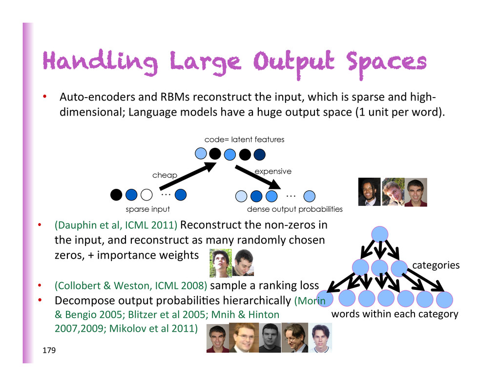
179. Handling Large Output Spaces   •  Auto-­‐encoders  and  RBMs  reconstruct  the  input,  which  is  sparse  and  high-­‐ dimensional;  Language  models  have  a  huge  output  space  (1  unit  per  word).         … code= latent features … sparse input dense output probabilities cheap expensive 179   categories   words  within  each  category     •  (Dauphin  et  al,  ICML  2011)  Reconstruct  the  non-­‐zeros  in   the  input,  and  reconstruct  as  many  randomly  chosen   zeros,  +  importance  weights   •  (Collobert  &  Weston,  ICML  2008)  sample  a  ranking  loss   •  Decompose  output  probabili8es  hierarchically  (Morin   &  Bengio  2005;  Blitzer  et  al  2005;  Mnih  &  Hinton   2007,2009;  Mikolov  et  al  2011)      
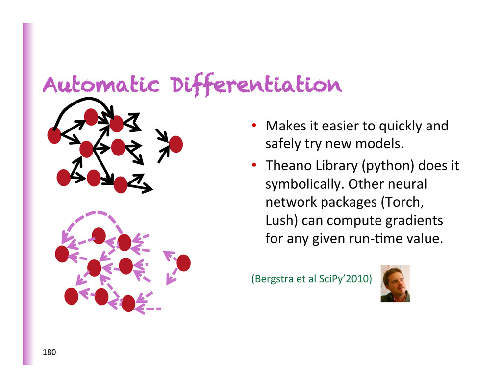
180. Automatic Differentiation •  Makes  it  easier  to  quickly  and   safely  try  new  models.   •  Theano  Library  (python)  does  it   symbolically.  Other  neural   network  packages  (Torch,   Lush)  can  compute  gradients   for  any  given  run-­‐8me  value.   (Bergstra  et  al  SciPy’2010)   180  
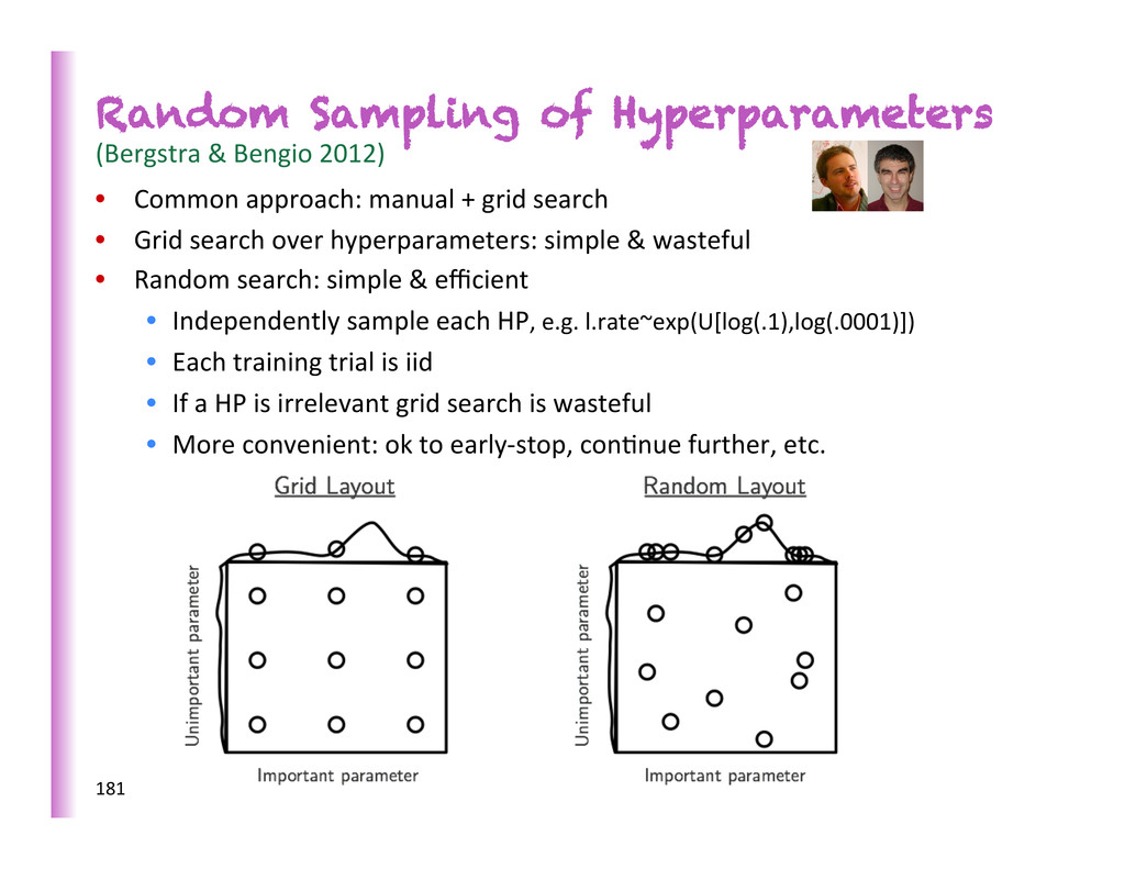
181. Random Sampling of Hyperparameters (Bergstra  &  Bengio  2012)   •  Common  approach:  manual  +  grid  search   •  Grid  search  over  hyperparameters:  simple  &  wasteful   •  Random  search:  simple  &  efficient   •  Independently  sample  each  HP,  e.g.  l.rate~exp(U[log(.1),log(.0001)])   •  Each  training  trial  is  iid   •  If  a  HP  is  irrelevant  grid  search  is  wasteful   •  More  convenient:  ok  to  early-­‐stop,  con8nue  further,  etc.   181  
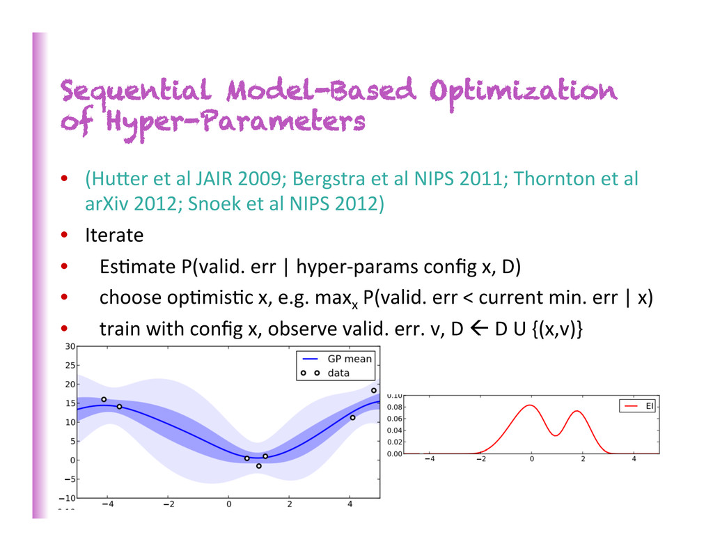
182. Sequential Model-Based Optimization of Hyper-Parameters •  (Huber  et  al  JAIR  2009;  Bergstra  et  al  NIPS  2011;  Thornton  et  al   arXiv  2012;  Snoek  et  al  NIPS  2012)   •  Iterate   •       Es8mate  P(valid.  err  |  hyper-­‐params  config  x,  D)   •       choose  op8mis8c  x,  e.g.  maxx  P(valid.  err  <  current  min.  err  |  x)   •       train  with  config  x,  observe  valid.  err.  v,  D  ß  D  U  {(x,v)}   182  
183. Discussion 183  
184. Concerns •  Many  algorithms  and  variants  (burgeoning  field)   •  Hyper-­‐parameters  (layer  size,  regulariza8on,  possibly   learning  rate)   •  Use  mul8-­‐core  machines,  clusters  and  random   sampling  for  cross-­‐valida8on  or  sequen8al  model-­‐ based  op8miza8on   184  
185. Concerns •  Slower  to  train  than  linear  models     •  Only  by  a  small  constant  factor,  and  much  more  compact   than  non-­‐parametric  (e.g.  n-­‐gram  models  or  kernel  machines)     •  Very  fast  during  inference/test  8me  (feed-­‐forward  pass  is  just   a  few  matrix  mul8plies)   •  Need  more  training  data?   •  Can  handle  and  benefit  from  more  training  data  (esp.   unlabeled),  suitable  for  Big  Data  (Google  trains  nets  with  a   billion  connec8ons,  [Le  et  al,  ICML  2012;  Dean  et  al  NIPS  2012])   •  Actually  needs  less  labeled  data   185  
186. Concern: non-convex optimization •  Can  ini8alize  system  with  convex  learner   •  Convex  SVM   •  Fixed  feature  space   •  Then  op8mize  non-­‐convex  variant  (add  and  tune  learned   features),  can’t  be  worse  than  convex  learner   186  
187. Challenges & Questions Part  4   187  
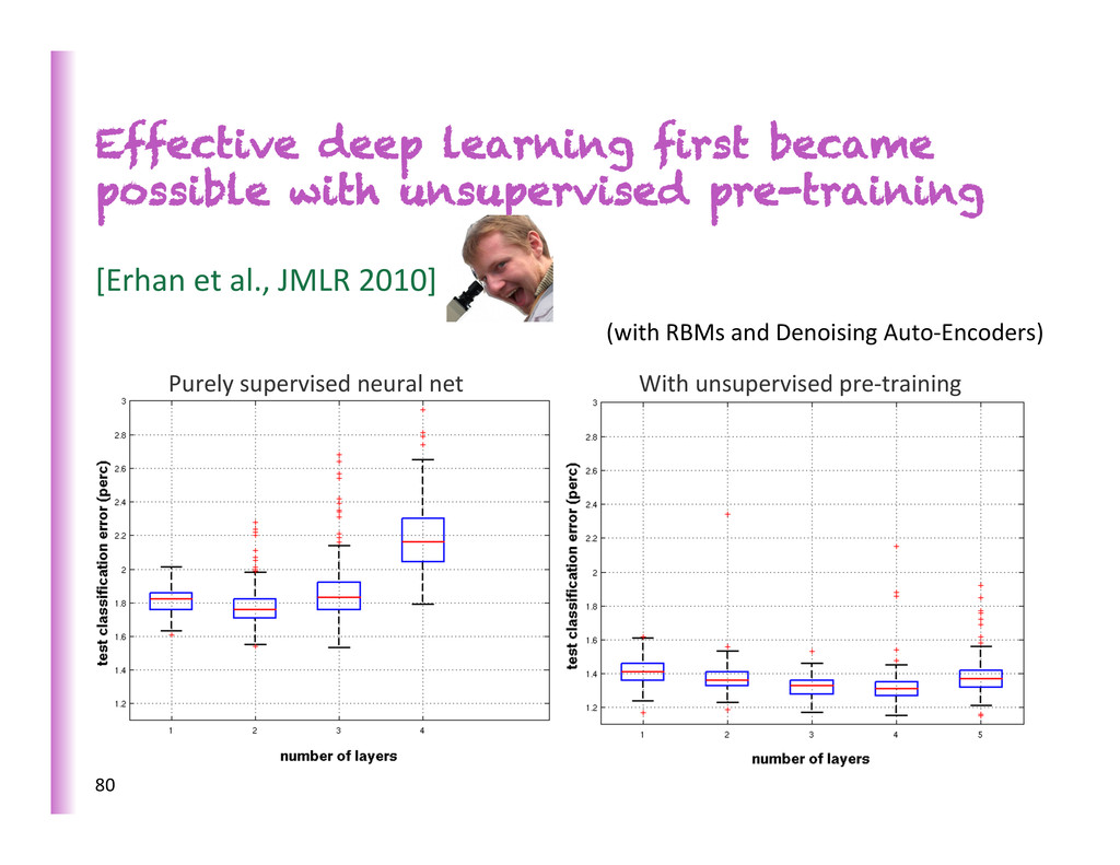
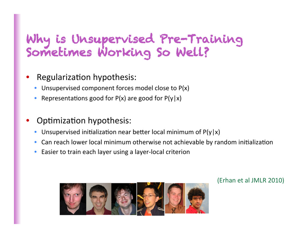
188. Why is Unsupervised Pre-Training Sometimes Working So Well? •  Regulariza8on  hypothesis:     •  Unsupervised  component  forces  model  close  to  P(x)   •  Representa8ons  good  for  P(x)  are  good  for  P(y|x)   •  Op8miza8on  hypothesis:   •  Unsupervised  ini8aliza8on  near  beber  local  minimum  of  P(y|x)   •  Can  reach  lower  local  minimum  otherwise  not  achievable  by  random  ini8aliza8on   •  Easier  to  train  each  layer  using  a  layer-­‐local  criterion   (Erhan  et  al  JMLR  2010)  
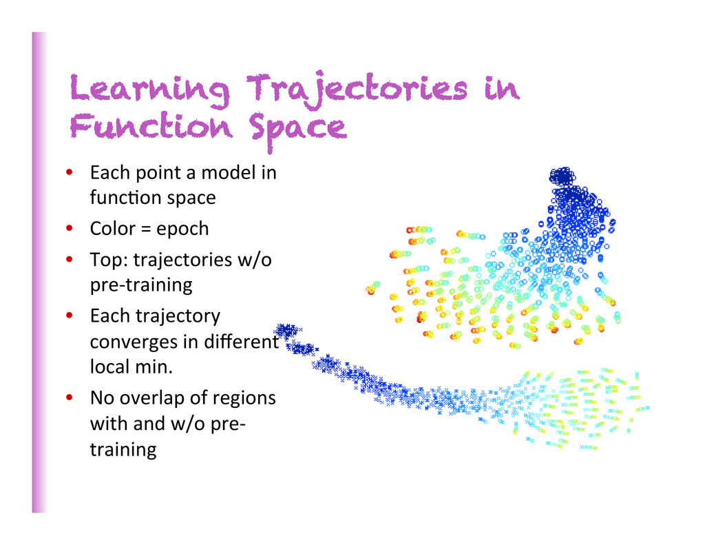
189. Learning Trajectories in Function Space •  Each  point  a  model  in   func8on  space   •  Color  =  epoch   •  Top:  trajectories  w/o   pre-­‐training   •  Each  trajectory   converges  in  different   local  min.   •  No  overlap  of  regions   with  and  w/o  pre-­‐ training  
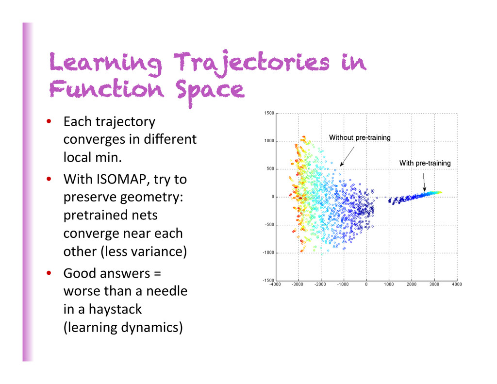
190. Learning Trajectories in Function Space •  Each  trajectory   converges  in  different   local  min.   •  With  ISOMAP,  try  to   preserve  geometry:                 pretrained  nets   converge  near  each   other  (less  variance)   •  Good  answers  =   worse  than  a  needle   in  a  haystack   (learning  dynamics)  
191. Deep Learning Challenges (Bengio, arxiv 1305.0445 Deep learning of representations: looking forward) •  Computa8onal  Scaling   •  Op8miza8on  &  Underfi€ng   •  Approximate  Inference  &  Sampling   •  Disentangling  Factors  of  Varia8on   •  Reasoning  &  One-­‐Shot  Learning  of  Facts   191  
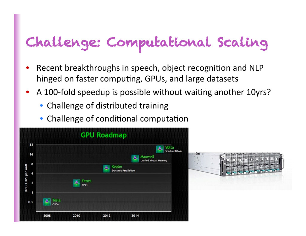
192. Challenge: Computational Scaling •  Recent  breakthroughs  in  speech,  object  recogni8on  and  NLP   hinged  on  faster  compu8ng,  GPUs,  and  large  datasets   •  A  100-­‐fold  speedup  is  possible  without  wai8ng  another  10yrs?   •  Challenge  of  distributed  training   •  Challenge  of  condi8onal  computa8on   192  
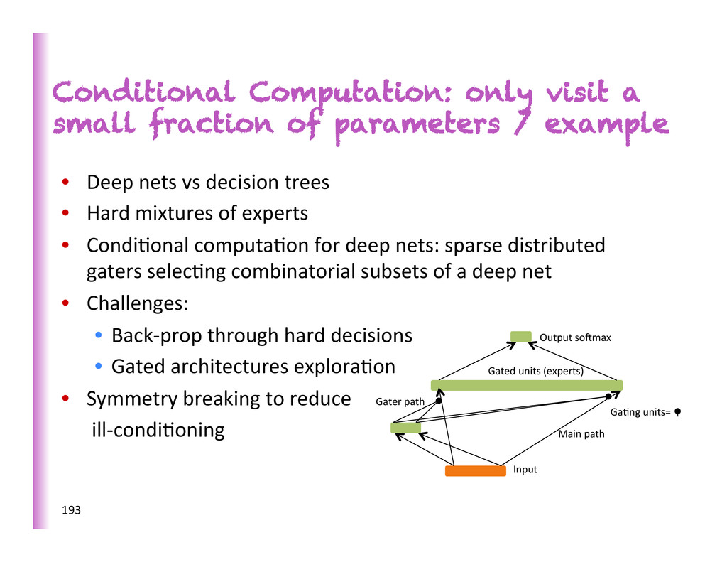
193. Output"so)max" Input" Gater"path" Main"path" Gated"units"(experts)" Ga8ng"units=" Conditional Computation: only visit a small fraction of parameters / example •  Deep  nets  vs  decision  trees   •  Hard  mixtures  of  experts   •  Condi8onal  computa8on  for  deep  nets:  sparse  distributed   gaters  selec8ng  combinatorial  subsets  of  a  deep  net   •  Challenges:   •  Back-­‐prop  through  hard  decisions   •  Gated  architectures  explora8on   •  Symmetry  breaking  to  reduce              ill-­‐condi8oning   193  
194. Distributed Training •  Minibatches  (too  large  =  slow  down)   •  Large  minibatches  +  2nd  order  methods   •  Asynchronous  SGD  (Bengio  et  al  2003,  Le  et  al  ICML  2012,  Dean  et  al  NIPS  2012)   •  Bobleneck:  sharing  weights/updates  among  nodes   •  New  ideas:   •  Low-­‐resolu8on  sharing  only  where  needed   •  Specialized  condi8onal  computa8on  (each  computer   specializes  in  updates  to  some  cluster  of  gated  experts,  and   prefers  examples  which  trigger  these  experts)   194  
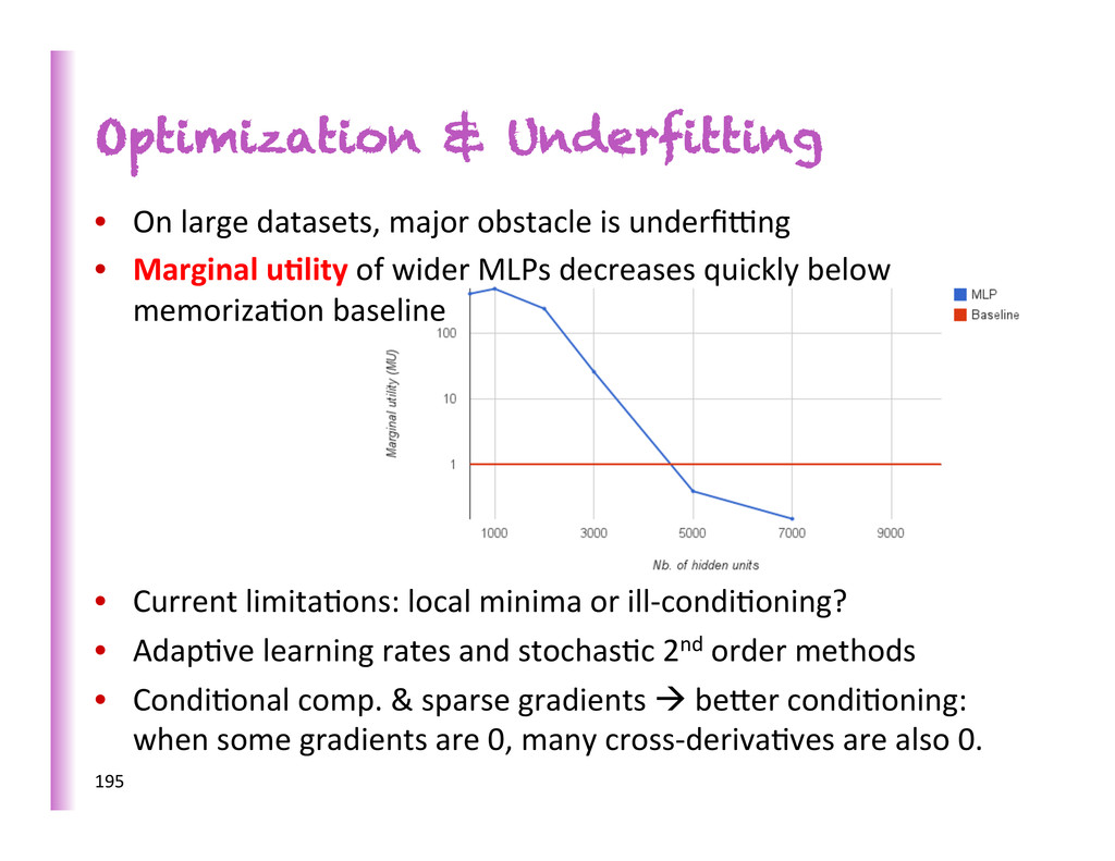
195. Optimization & Underfitting •  On  large  datasets,  major  obstacle  is  underfi€ng   •  Marginal  u0lity  of  wider  MLPs  decreases  quickly  below   memoriza8on  baseline   •  Current  limita8ons:  local  minima  or  ill-­‐condi8oning?   •  Adap8ve  learning  rates  and  stochas8c  2nd  order  methods   •  Condi8onal  comp.  &  sparse  gradients  à  beber  condi8oning:   when  some  gradients  are  0,  many  cross-­‐deriva8ves  are  also  0.   195  
196.   •  Mixing   •  Local:  auto-­‐correla8on  between  successive  samples   •  Global:  mixing  between  major  “modes”     MCMC Sampling Challenges •  Burn-­‐in   •  Going  from  an  unlikely  configura8on  to  likely  ones     196   challenge  
197. For gradient & inference: More difficult to mix with better trained models •  Early  during  training,  density  smeared  out,  mode  bumps  overlap   •  Later  on,  hard  to  cross  empty  voids  between  modes   197   Are  we  doomed  if   we  rely  on  MCMC   during  training?   Will  we  be  able  to   train  really  large  &   complex  models?     Training  updates   Mixing   vicious  circle  
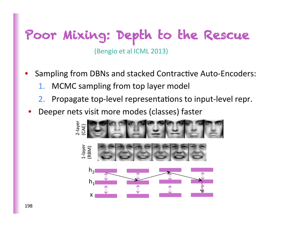
198. Poor Mixing: Depth to the Rescue •  Sampling  from  DBNs  and  stacked  Contrac8ve  Auto-­‐Encoders:   1.  MCMC  sampling  from  top  layer  model   2.  Propagate  top-­‐level  representa8ons  to  input-­‐level  repr.   •  Deeper  nets  visit  more  modes  (classes)  faster   198   x   h2   h1   1-­‐layer     (RBM)   2-­‐layer     (CAE)   (Bengio  et  al  ICML  2013)  
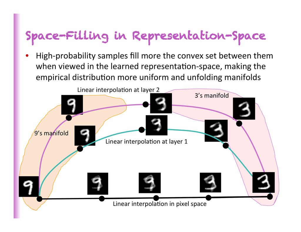
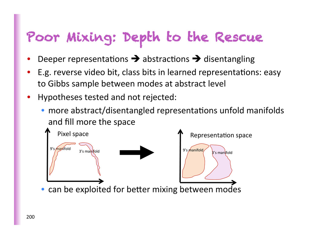
199. Space-Filling in Representation-Space •  High-­‐probability  samples  fill  more  the  convex  set  between  them   when  viewed  in  the  learned  representa8on-­‐space,  making  the   empirical  distribu8on  more  uniform  and  unfolding  manifolds   Linear  interpola8on  at  layer  1   Linear  interpola8on  at  layer  2   3’s  manifold   9’s  manifold   Linear  interpola8on  in  pixel  space  
200. Poor Mixing: Depth to the Rescue •  Deeper  representa8ons  è  abstrac8ons  è  disentangling   •  E.g.  reverse  video  bit,  class  bits  in  learned  representa8ons:  easy   to  Gibbs  sample  between  modes  at  abstract  level   •  Hypotheses  tested  and  not  rejected:     •  more  abstract/disentangled  representa8ons  unfold  manifolds   and  fill  more  the  space     •  can  be  exploited  for  beber  mixing  between  modes   200   Pixel  space   9’s  manifold   3’s  manifold   Representa8on  space   9’s  manifold   3’s  manifold  
201. Inference Challenges •  Many  latent  variables  involved  in  understanding   complex  inputs  (e.g.  in  NLP:  sense  ambiguity,  parsing,   seman8c  role)   •  Almost  any  inference  mechanism  can  be  combined   with  deep  learning   •  See  [Bobou,  LeCun,  Bengio  97],  [Graves  2012]   •  Complex  inference  can  be  hard  (exponen8ally)  and   needs  to  be  approximate  à  learn  to  perform  inference   201  
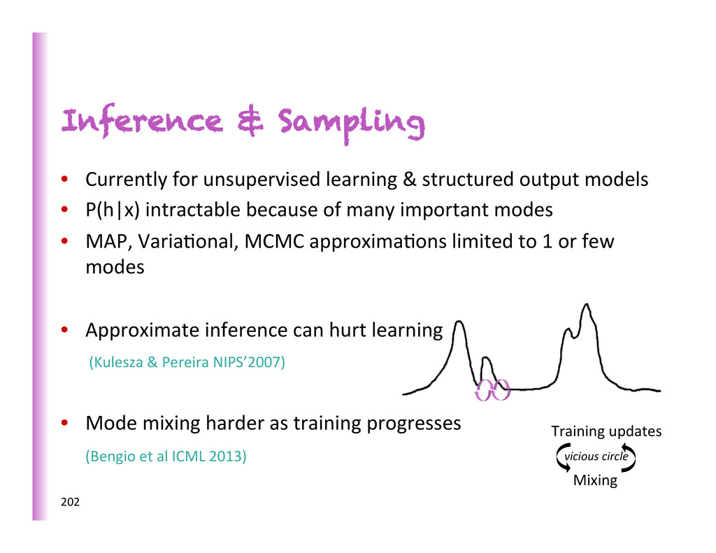
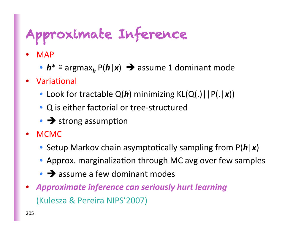
202. Inference & Sampling •  Currently  for  unsupervised  learning  &  structured  output  models   •  P(h|x)  intractable  because  of  many  important  modes   •  MAP,  Varia8onal,  MCMC  approxima8ons  limited  to  1  or  few   modes   •  Approximate  inference  can  hurt  learning              (Kulesza  &  Pereira  NIPS’2007)   •  Mode  mixing  harder  as  training  progresses              (Bengio  et  al  ICML  2013)   202   Training  updates   Mixing   vicious  circle  
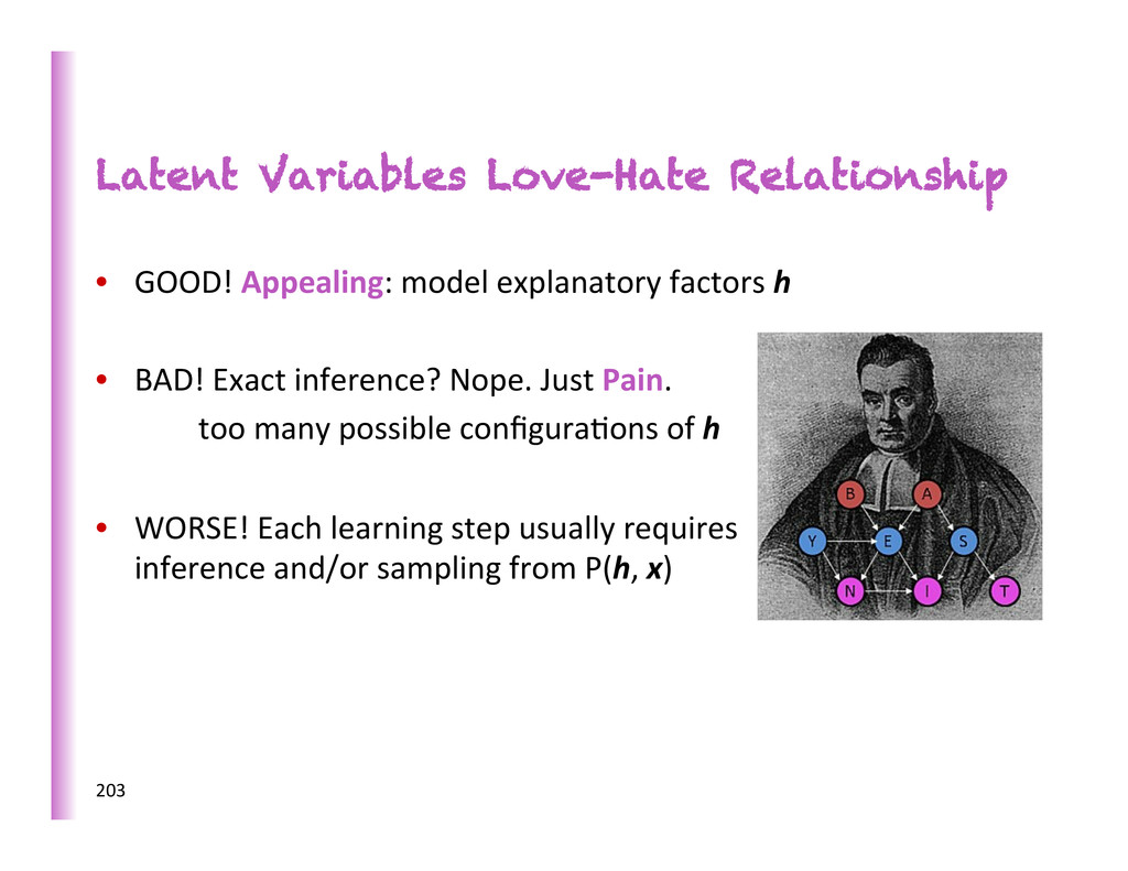
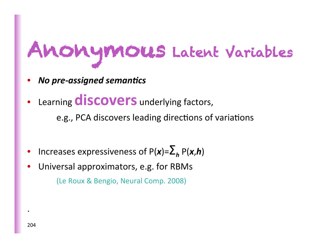
203. Latent Variables Love-Hate Relationship •  GOOD!  Appealing:  model  explanatory  factors  h   •  BAD!  Exact  inference?  Nope.  Just  Pain.    too  many  possible  configura8ons  of  h     •  WORSE!  Each  learning  step  usually  requires   inference  and/or  sampling  from  P(h,  x)   203  
204. Anonymous Latent Variables •  No  pre-­‐assigned  seman#cs   •  Learning  discovers  underlying  factors,      e.g.,  PCA  discovers  leading  direc8ons  of  varia8ons       •  Increases  expressiveness  of  P(x)=Σ h  P(x,h)   •  Universal  approximators,  e.g.  for  RBMs      (Le  Roux  &  Bengio,  Neural  Comp.  2008)   .   204  
205. Approximate Inference •  MAP   •  h*  ≅  argmaxh  P(h|x)    è  assume  1  dominant  mode   •  Varia8onal   •  Look  for  tractable  Q(h)  minimizing  KL(Q(.)||P(.|x))     •  Q  is  either  factorial  or  tree-­‐structured   •  è  strong  assump8on   •  MCMC   •  Setup  Markov  chain  asympto8cally  sampling  from  P(h|x)   •  Approx.  marginaliza8on  through  MC  avg  over  few  samples   •  è  assume  a  few  dominant  modes     •  Approximate  inference  can  seriously  hurt  learning            (Kulesza  &  Pereira  NIPS’2007)   205  
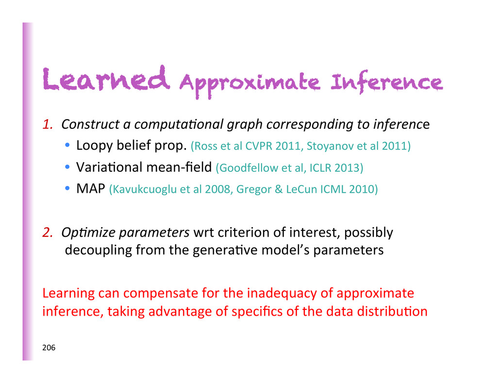
206. Learned Approximate Inference 1.  Construct  a  computaKonal  graph  corresponding  to  inference   •  Loopy  belief  prop.  (Ross  et  al  CVPR  2011,  Stoyanov  et  al  2011)     •  Varia8onal  mean-­‐field  (Goodfellow  et  al,  ICLR  2013)     •  MAP  (Kavukcuoglu  et  al  2008,  Gregor  &  LeCun  ICML  2010)     2.  OpKmize  parameters  wrt  criterion  of  interest,  possibly   decoupling  from  the  genera8ve  model’s  parameters   Learning  can  compensate  for  the  inadequacy  of  approximate   inference,  taking  advantage  of  specifics  of  the  data  distribu8on       206  
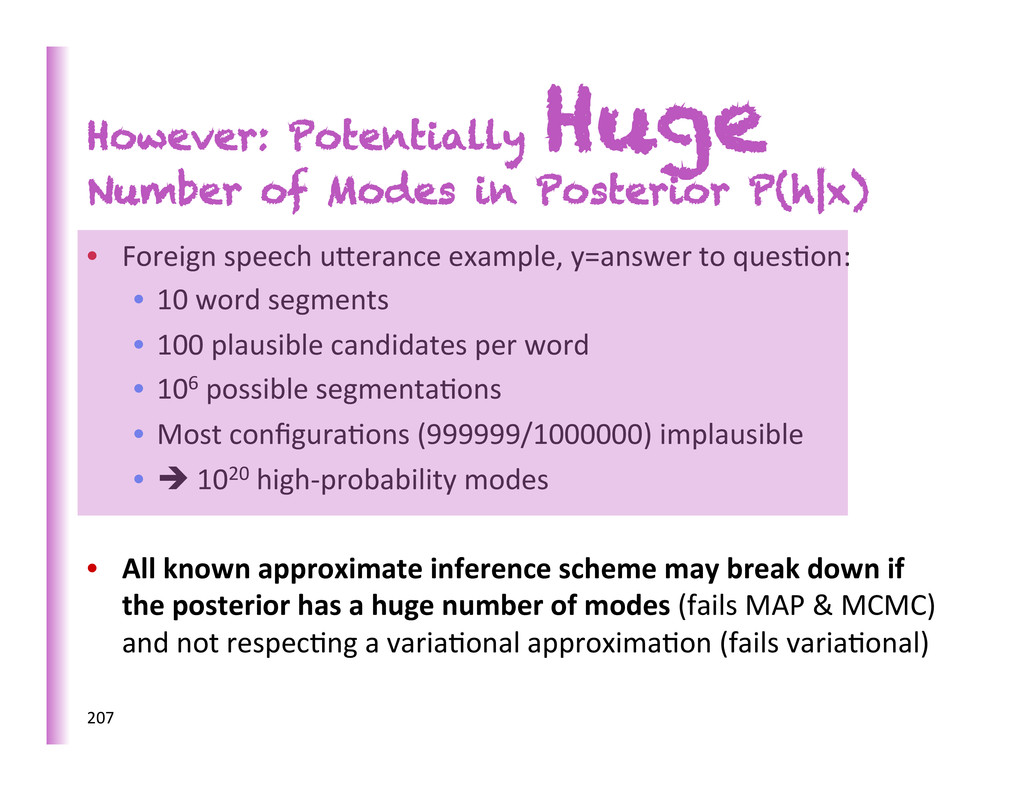
207. However: Potentially Huge Number of Modes in Posterior P(h|x) •  Foreign  speech  uberance  example,  y=answer  to  ques8on:   •  10  word  segments   •  100  plausible  candidates  per  word   •  106  possible  segmenta8ons   •  Most  configura8ons  (999999/1000000)  implausible   •  è  1020  high-­‐probability  modes   •  All  known  approximate  inference  scheme  may  break  down  if   the  posterior  has  a  huge  number  of  modes  (fails  MAP  &  MCMC)   and  not  respec8ng  a  varia8onal  approxima8on  (fails  varia8onal)     207  
208. Hint •  Deep  neural  nets  learn  good  P(y|x)  classifiers  even  if  there  are   poten8ally  many  true  latent  variables  involved   •  Exploits  structure  in  P(y|x)  that  persist  even  aZer  summing  h     •  But  how  do  we  generalize  this  idea  to  full  joint-­‐distribu8on   learning  and  answering  any  ques8on  about  these  variables,  not   just  one?   208  
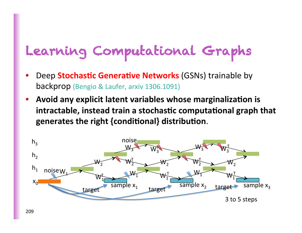
209. Learning Computational Graphs •  Deep  Stochas0c  Genera0ve  Networks  (GSNs)  trainable  by   backprop  (Bengio  &  Laufer,  arxiv  1306.1091)   •  Avoid  any  explicit  latent  variables  whose  marginaliza0on  is   intractable,  instead  train  a  stochas0c  computa0onal  graph  that   generates  the  right  {condi0onal}  distribu0on.   209   1" x 0" h 3" h 2" h 1" W 1" W 1" W 1" T" W 1" W 2" W 2" T" W 3" W 1" T" W 1" T" W 2" W 2" T" W 2" W 3" T" W 3" W 3" T" sample"x 1 " sample"x 2 " sample"x 3 " target" target" target" noise   noise   3  to  5  steps  
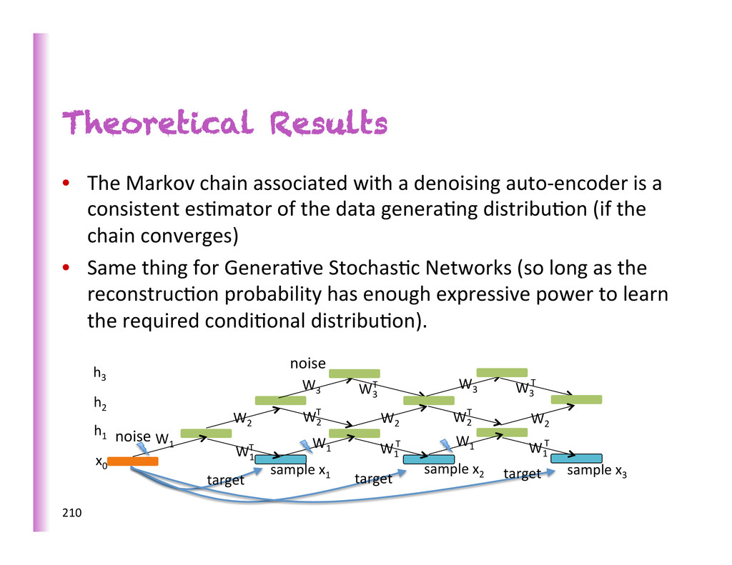
210. Theoretical Results •  The  Markov  chain  associated  with  a  denoising  auto-­‐encoder  is  a   consistent  es8mator  of  the  data  genera8ng  distribu8on  (if  the   chain  converges)   •  Same  thing  for  Genera8ve  Stochas8c  Networks  (so  long  as  the   reconstruc8on  probability  has  enough  expressive  power  to  learn   the  required  condi8onal  distribu8on).   210   1" x 0" h 3" h 2" h 1" W 1" W 1" W 1" T" W 1" W 2" W 2" T" W 3" W 1" T" W 1" T" W 2" W 2" T" W 2" W 3" T" W 3" W 3" T" sample"x 1 " sample"x 2 " sample"x 3 " target" target" target" noise   noise  
211. GSN Experiments: validating the theorem in a continuous non-parametric setting 211  
212. GSN Experiments: Consecutive Samples 212   Filling-­‐in  the  LHS  
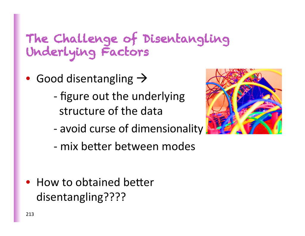
213. The Challenge of Disentangling Underlying Factors •  Good  disentangling  à      -­‐  figure  out  the  underlying              structure  of  the  data    -­‐  avoid  curse  of  dimensionality    -­‐  mix  beber  between  modes     •  How  to  obtained  beber   disentangling????   213  
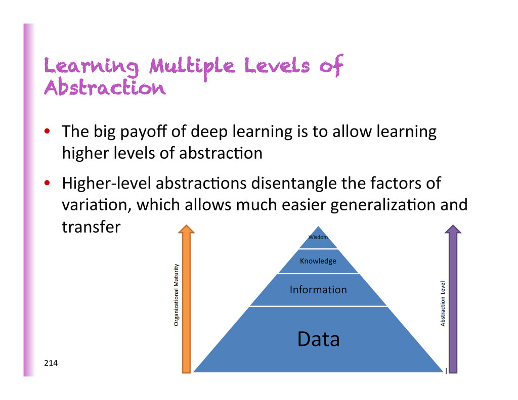
214. Learning Multiple Levels of Abstraction •  The  big  payoff  of  deep  learning  is  to  allow  learning   higher  levels  of  abstrac8on   •  Higher-­‐level  abstrac8ons  disentangle  the  factors  of   varia8on,  which  allows  much  easier  generaliza8on  and   transfer   214  
215. If Time Permits… 215  
216. Culture vs Effective Local Minima 216   Issue:  underfirng  due  to  combinatorially  many  poor   effec#ve  local  minima   Bengio  2013  (also  arXiv  2012)   where  the  op8mizer  gets  stuck  
217. Hypothesis 1 •  When  the  brain  of  a  single  biological  agent  learns,  it  performs  an   approximate  op8miza8on  with  respect  to  some  endogenous   objec8ve.   217   Hypothesis 2 •  When  the  brain  of  a  single  biological  agent  learns,  it  relies  on   approximate  local  descent  in  order  to  gradually  improve  itself.  
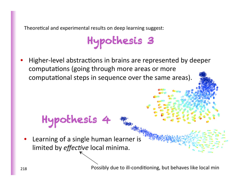
218. Hypothesis 3 •  Higher-­‐level  abstrac8ons  in  brains  are  represented  by  deeper   computa8ons  (going  through  more  areas  or  more   computa8onal  steps  in  sequence  over  the  same  areas).   218   Hypothesis 4 •  Learning  of  a  single  human  learner  is   limited  by  effecKve  local  minima.   Theore8cal  and  experimental  results  on  deep  learning  suggest:   Possibly  due  to  ill-­‐condi8oning,  but  behaves  like  local  min  
219. Hypothesis 5 •  A  single  human  learner  is  unlikely  to  discover  high-­‐level   abstrac8ons  by  chance  because  these  are  represented  by  a  deep   sub-­‐network  in  the  brain.   219   Hypothesis 6 •  A  human  brain  can  learn  high-­‐level  abstrac8ons  if  guided  by  the   signals  produced  by  other  humans,  which  act  as  hints  or  indirect   supervision  for  these  high-­‐level  abstrac8ons.   Suppor8ng  evidence:  (Gulcehre  &  Bengio  ICLR  2013)  
220. How is one brain transferring abstractions to another brain? 220   … … … … … … … … … … … … Shared  input  X   Linguis8c  exchange   =  8ny  /  noisy  channel   Linguis8c   representa8on   Linguis8c   representa8on  
221. How do we escape local minima? •  linguis8c  inputs  =  extra  examples,  summarize   knowledge     •  criterion  landscape  easier  to  op8mize  (e.g.   curriculum  learning)   •  turn  difficult  unsupervised  learning  into  easy   supervised  learning  of  intermediate  abstrac8ons   221  
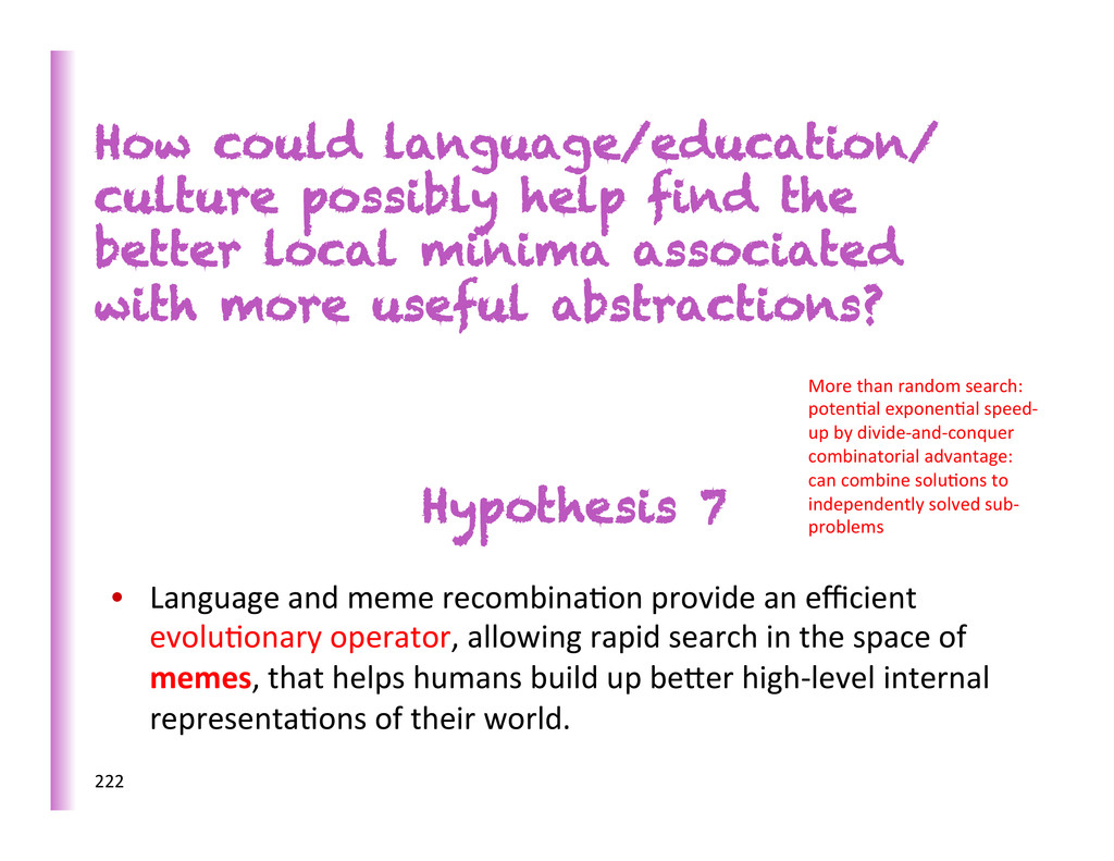
222. 222   Hypothesis 7 •  Language  and  meme  recombina8on  provide  an  efficient   evolu8onary  operator,  allowing  rapid  search  in  the  space  of   memes,  that  helps  humans  build  up  beber  high-­‐level  internal   representa8ons  of  their  world.   How could language/education/ culture possibly help find the better local minima associated with more useful abstractions? More  than  random  search:     poten8al  exponen8al  speed-­‐ up  by  divide-­‐and-­‐conquer   combinatorial  advantage:   can  combine  solu8ons  to   independently  solved  sub-­‐ problems  
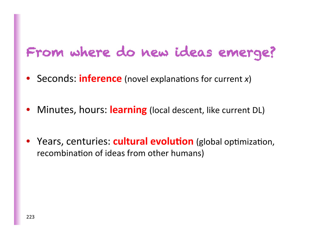
223. From where do new ideas emerge? •  Seconds:  inference  (novel  explana8ons  for  current  x)   •  Minutes,  hours:  learning  (local  descent,  like  current  DL)   •  Years,  centuries:  cultural  evolu0on  (global  op8miza8on,   recombina8on  of  ideas  from  other  humans)   223  
224. Related Tutorials •  Deep  Learning  tutorials  (python):  hbp://deeplearning.net/tutorials   •  Stanford  deep  learning  tutorials  with  simple  programming   assignments  and  reading  list   hbp://deeplearning.stanford.edu/wiki/   •  ACL  2012  Deep  Learning  for  NLP  tutorial   hbp://www.socher.org/index.php/DeepLearningTutorial/   •  ICML  2012  Representa8on  Learning  tutorial   hbp://www.iro.umontreal.ca/~bengioy/talks/deep-­‐learning-­‐ tutorial-­‐2012.html   •  IPAM  2012  Summer  school  on  Deep  Learning   hbp://www.iro.umontreal.ca/~bengioy/talks/deep-­‐learning-­‐tutorial-­‐ aaai2013.html   •  More  reading:  Paper  references  in  separate  pdf,  on  my  web  page   224  
225. Software •  Theano  (Python  CPU/GPU)  mathema8cal  and  deep  learning   library  hbp://deeplearning.net/soZware/theano   •  Can  do  automa8c,  symbolic  differen8a8on   •  Senna:  POS,  Chunking,  NER,  SRL   •  by  Collobert  et  al.  hbp://ronan.collobert.com/senna/   •  State-­‐of-­‐the-­‐art  performance  on  many  tasks   •  3500  lines  of  C,  extremely  fast  and  using  very  lible  memory   •  Torch  ML  Library  (C++  +  Lua)  hbp://www.torch.ch/   •  Recurrent  Neural  Network  Language  Model   hbp://www.fit.vutbr.cz/~imikolov/rnnlm/   •  Recursive  Neural  Net  and  RAE  models  for  paraphrase  detec8on,   sen8ment  analysis,  rela8on  classifica8on  www.socher.org   225  
226. Software: what’s next •  Off-­‐the-­‐shelf  SVM  packages  are  useful  to  researchers   from  a  wide  variety  of  fields  (no  need  to  understand   RKHS).   •  To  make  deep  learning  more  accessible:  release  off-­‐ the-­‐shelf  learning  packages  that  handle  hyper-­‐ parameter  op8miza8on,  exploi8ng  mul8-­‐core  or   cluster  at  disposal  of  user.   •  Spearmint  (Snoek)   •  HyperOpt  (Bergstra)   226  
227. Conclusions •  Deep  Learning  &  Representa8on  Learning  have  matured   •  Int.  Conf.  on  Learning  Representa8on  2013  a  huge  success!   •  Industrial  strength  applica8ons  in  place  (Google,  MicrosoZ)   •  Room  for  more  research:   •  Scaling  computa8on  even  more   •  Beber  op8miza8on   •  Ge€ng  rid  of  intractable  inference  (in  the  works!)   •  Coaxing  the  models  into  more  disentangled  abstrac8ons   •  Learning  to  reason  from  incrementally  added  facts   227  
228. Merci! Questions? LISA team: