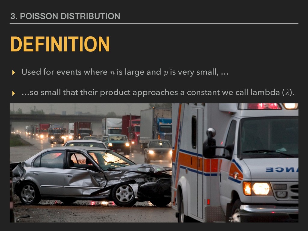
Lecture slides for Lecture 05 of the Saint Louis University Course Quantitative Analysis: Applied Inferential Statistics. These slides cover the binomial, poisson, and normal distributions and provide an introduction to statistical significance.
the next lecture. There was an update on the final project due today as an issue in your final project GitHub repo (DoeProject if your last name is “Doe”) 1. FRONT MATTER ANNOUNCEMENTS
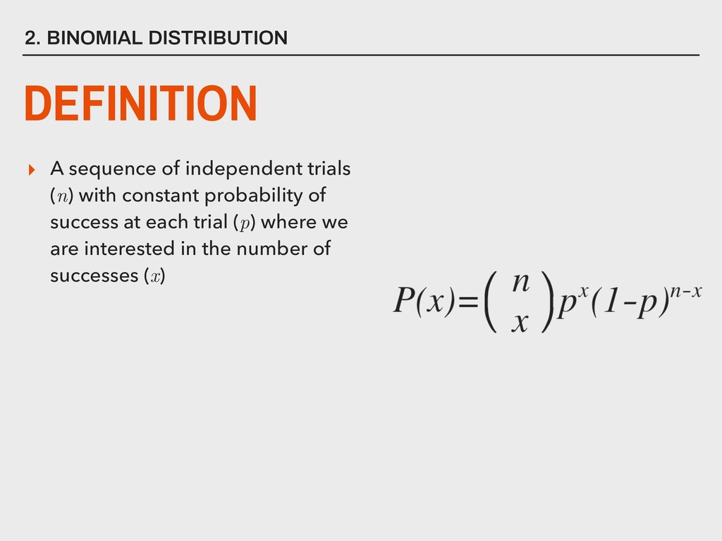
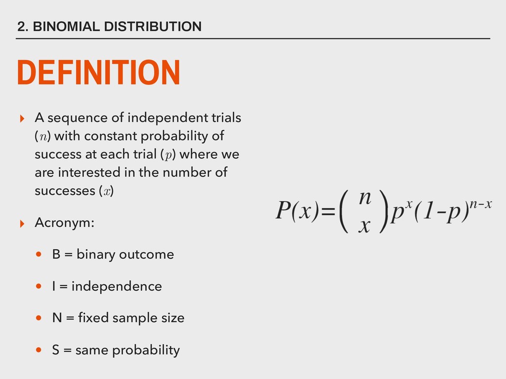
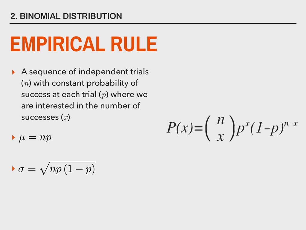
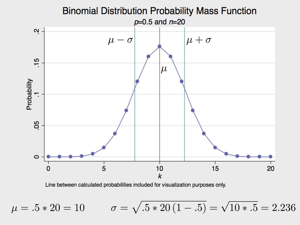
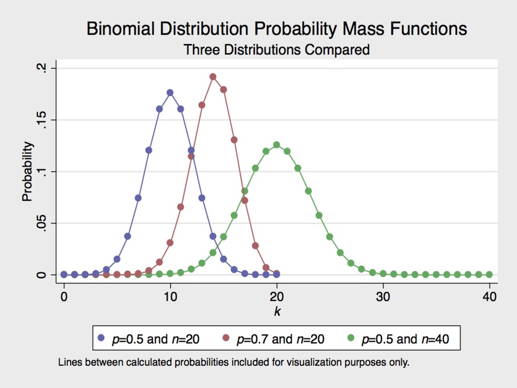
of success at each trial (p) where we are interested in the number of successes (x) ▸ Acronym: • B = binary outcome • I = independence • N = fixed sample size • S = same probability 2. BINOMIAL DISTRIBUTION DEFINITION
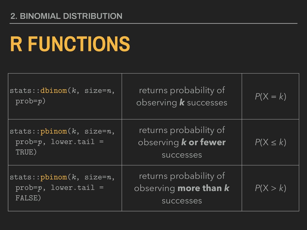
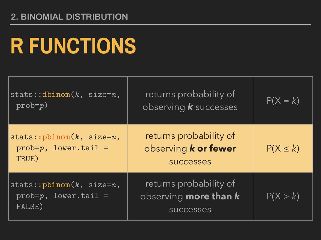
of observing k successes P(X = k) stats::pbinom(k, size=n, prob=p, lower.tail = TRUE) returns probability of observing k or fewer successes P(X ≤ k) stats::pbinom(k, size=n, prob=p, lower.tail = FALSE) returns probability of observing more than k successes P(X > k)
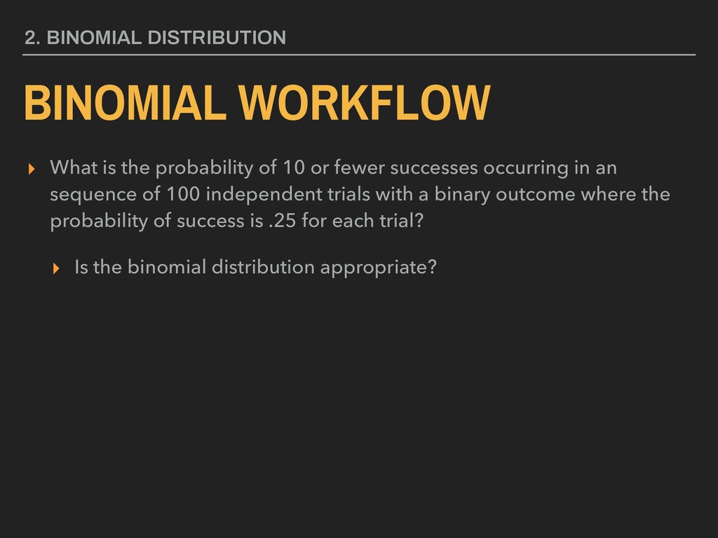
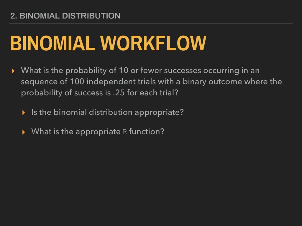
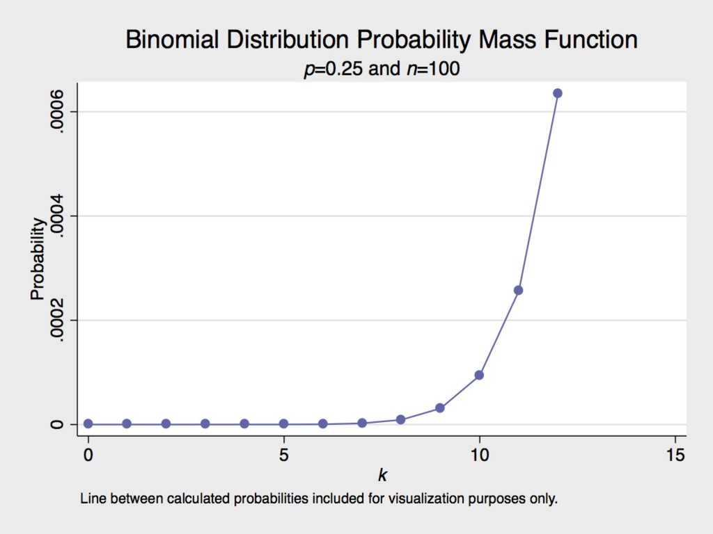
of 10 or fewer successes occurring in an sequence of 100 independent trials with a binary outcome where the probability of success is .25 for each trial? ▸ Is the binomial distribution appropriate?
of 10 or fewer successes occurring in an sequence of 100 independent trials with a binary outcome where the probability of success is .25 for each trial? ▸ Is the binomial distribution appropriate?
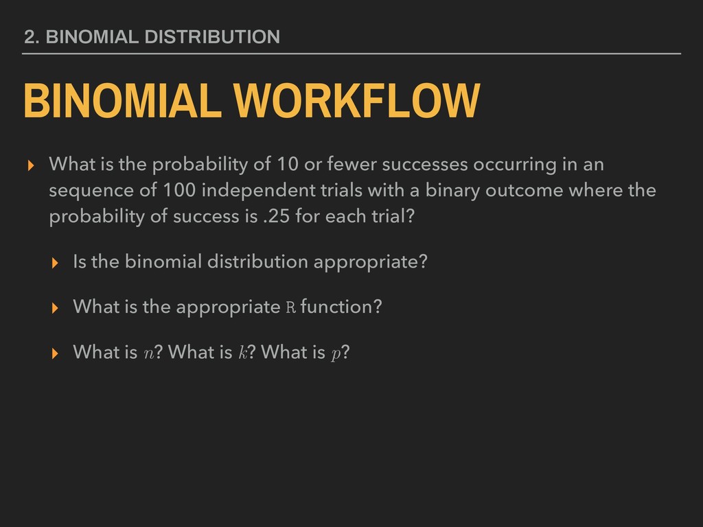
of 10 or fewer successes occurring in an sequence of 100 independent trials with a binary outcome where the probability of success is .25 for each trial? ▸ Is the binomial distribution appropriate? ▸ What is the appropriate R function?
of 10 or fewer successes occurring in an sequence of 100 independent trials with a binary outcome where the probability of success is .25 for each trial? ▸ Is the binomial distribution appropriate? ▸ What is the appropriate R function?
of observing k successes P(X = k) stats::pbinom(k, size=n, prob=p, lower.tail = TRUE) returns probability of observing k or fewer successes P(X ≤ k) stats::pbinom(k, size=n, prob=p, lower.tail = FALSE) returns probability of observing more than k successes P(X > k)
of observing k successes P(X = k) stats::pbinom(k, size=n, prob=p, lower.tail = TRUE) returns probability of observing k or fewer successes P(X ≤ k) stats::pbinom(k, size=n, prob=p, lower.tail = FALSE) returns probability of observing more than k successes P(X > k)
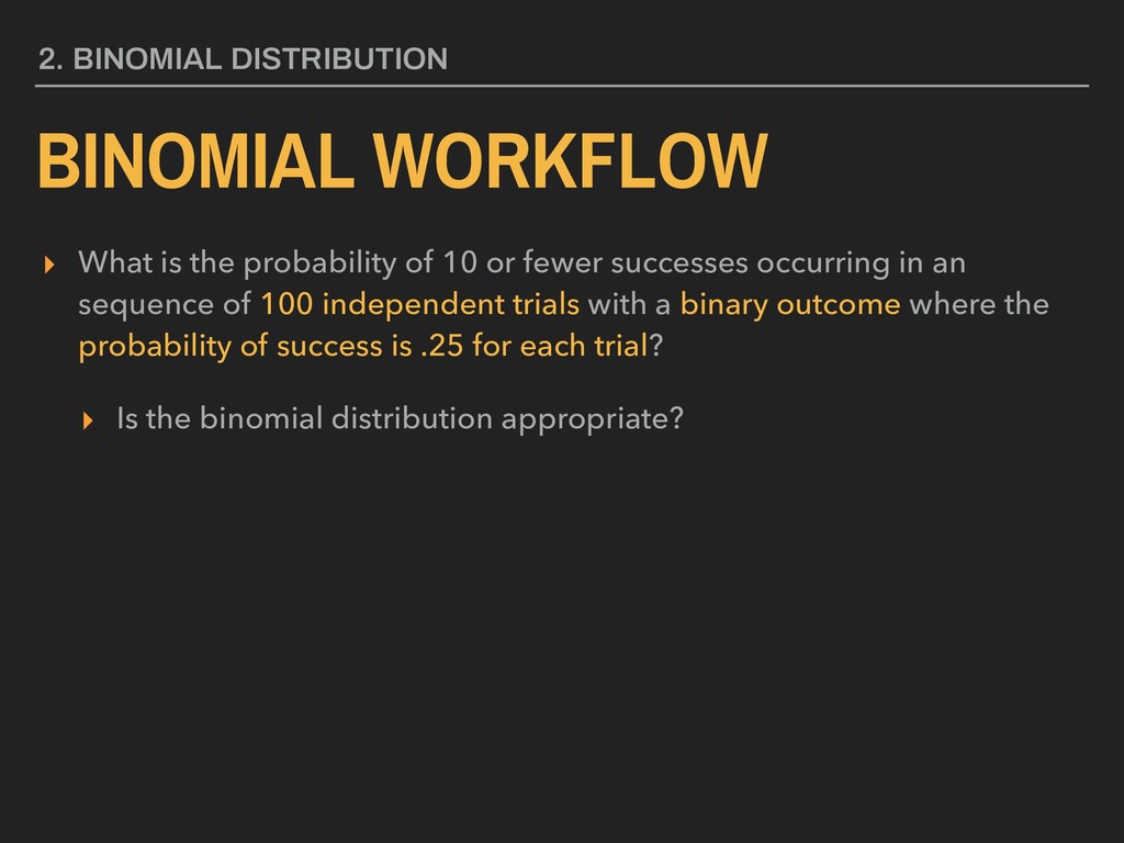
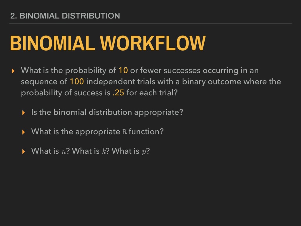
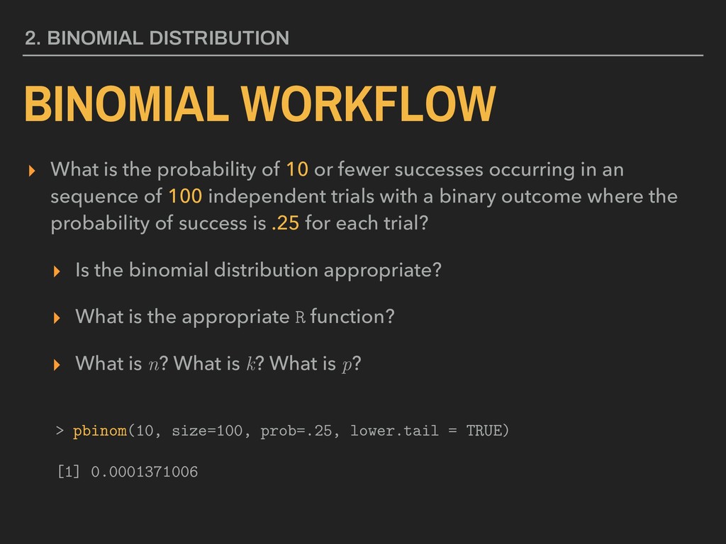
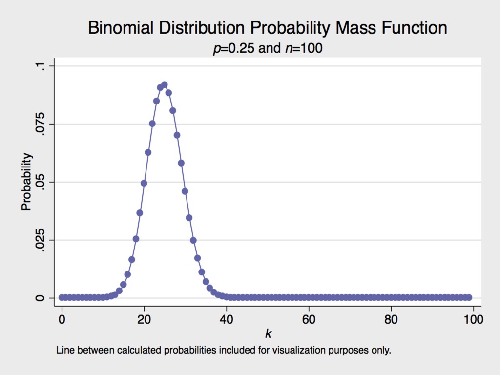
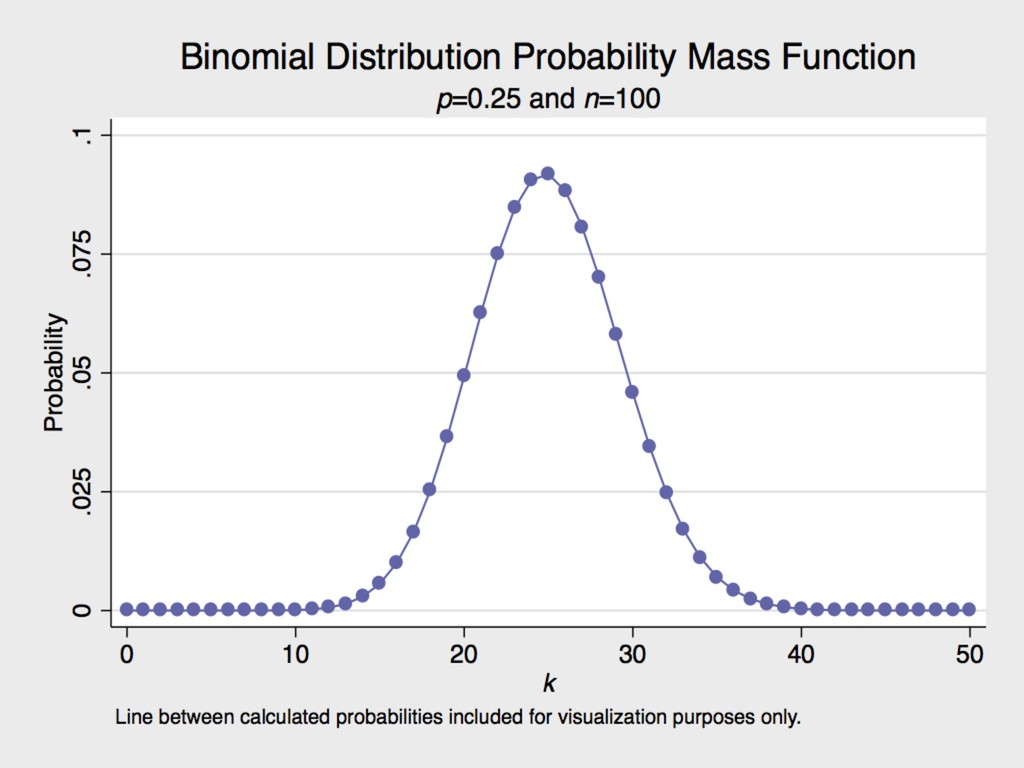
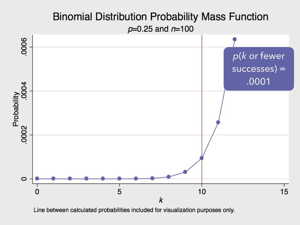
of 10 or fewer successes occurring in an sequence of 100 independent trials with a binary outcome where the probability of success is .25 for each trial? ▸ Is the binomial distribution appropriate? ▸ What is the appropriate R function? ▸ What is n? What is k? What is p?
of 10 or fewer successes occurring in an sequence of 100 independent trials with a binary outcome where the probability of success is .25 for each trial? ▸ Is the binomial distribution appropriate? ▸ What is the appropriate R function? ▸ What is n? What is k? What is p?
of 10 or fewer successes occurring in an sequence of 100 independent trials with a binary outcome where the probability of success is .25 for each trial? ▸ Is the binomial distribution appropriate? ▸ What is the appropriate R function? ▸ What is n? What is k? What is p? > pbinom(10, size=100, prob=.25, lower.tail = TRUE) [1] 0.0001371006
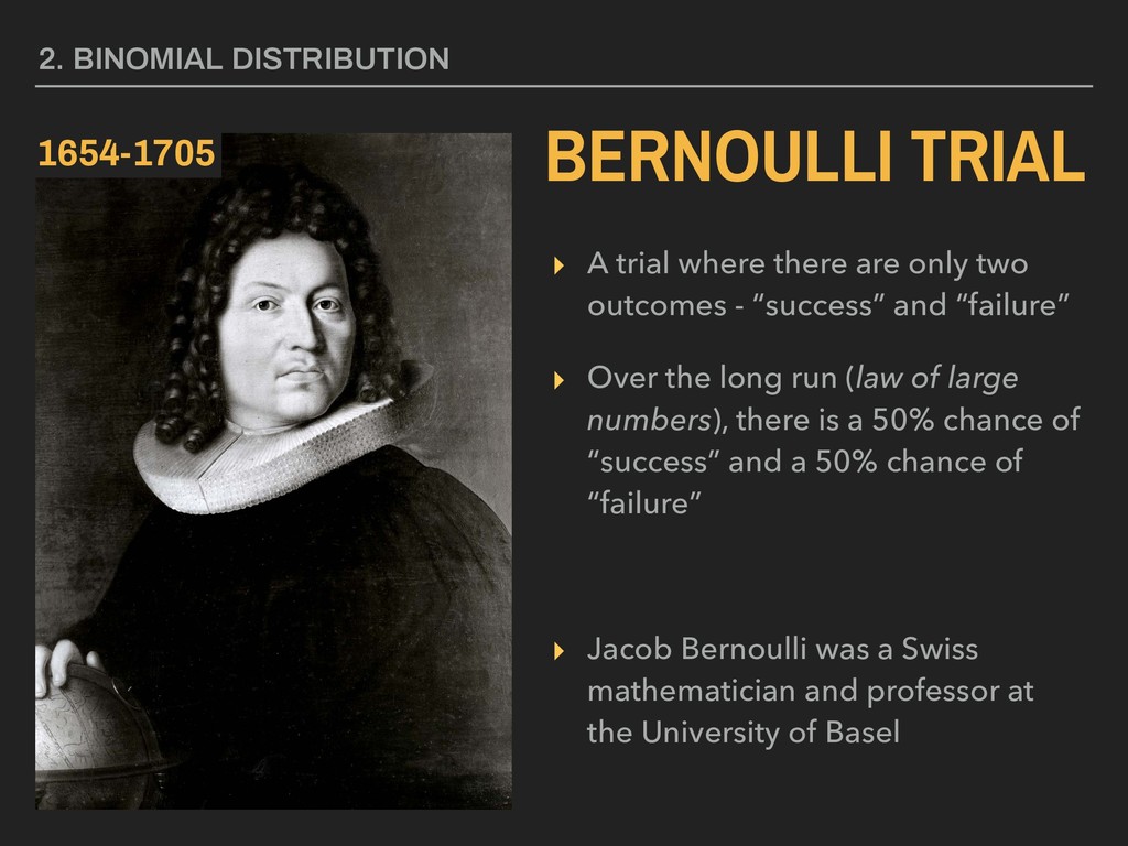
“success” and “failure” ▸ Over the long run (law of large numbers), there is a 50% chance of “success” and a 50% chance of “failure” ▸ Jacob Bernoulli was a Swiss mathematician and professor at the University of Basel 2. BINOMIAL DISTRIBUTION BERNOULLI TRIAL 1654-1705
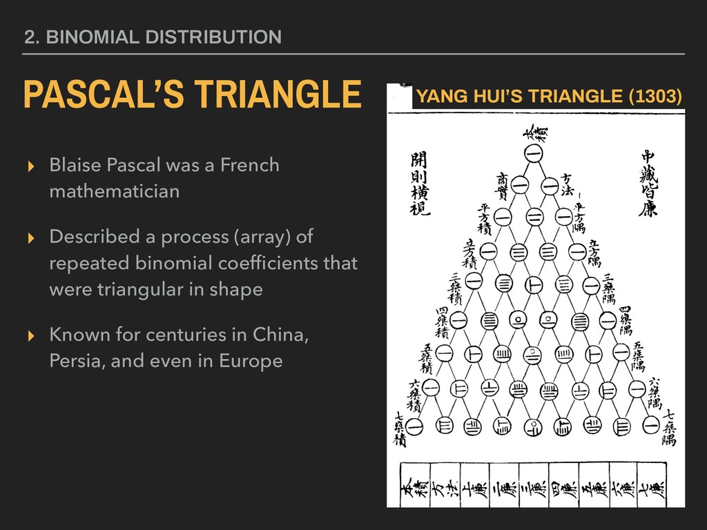
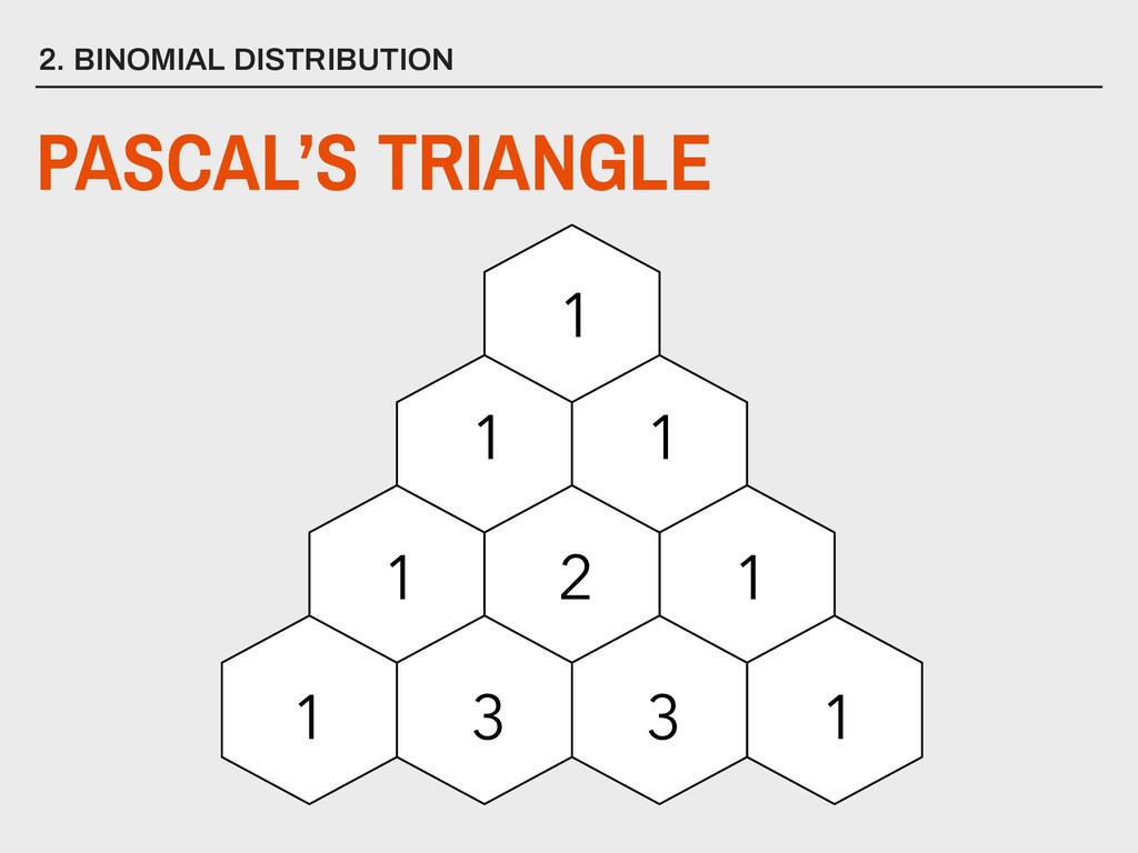
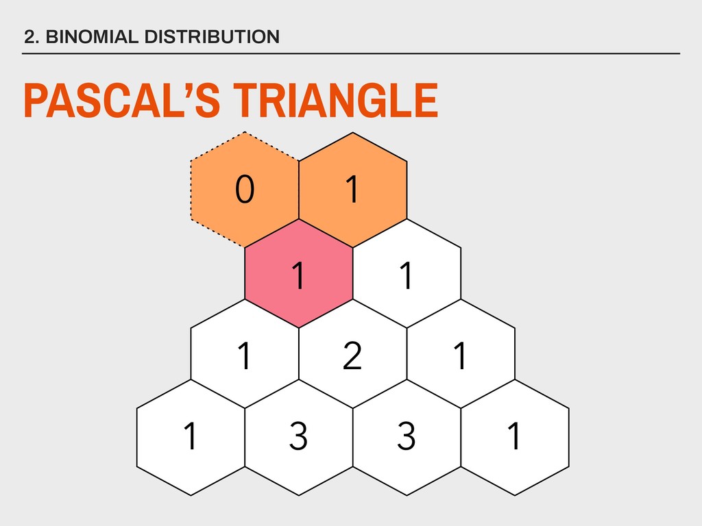
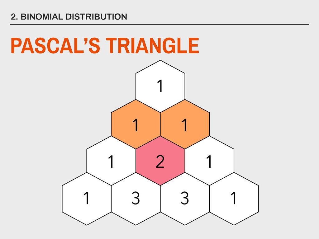
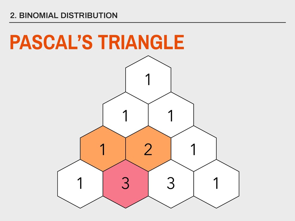
process (array) of repeated binomial coefficients that were triangular in shape ▸ Known for centuries in China, Persia, and even in Europe 2. BINOMIAL DISTRIBUTION PASCAL’S TRIANGLE 1623-1662
process (array) of repeated binomial coefficients that were triangular in shape ▸ Known for centuries in China, Persia, and even in Europe 2. BINOMIAL DISTRIBUTION PASCAL’S TRIANGLE YANG HUI’S TRIANGLE (1303)
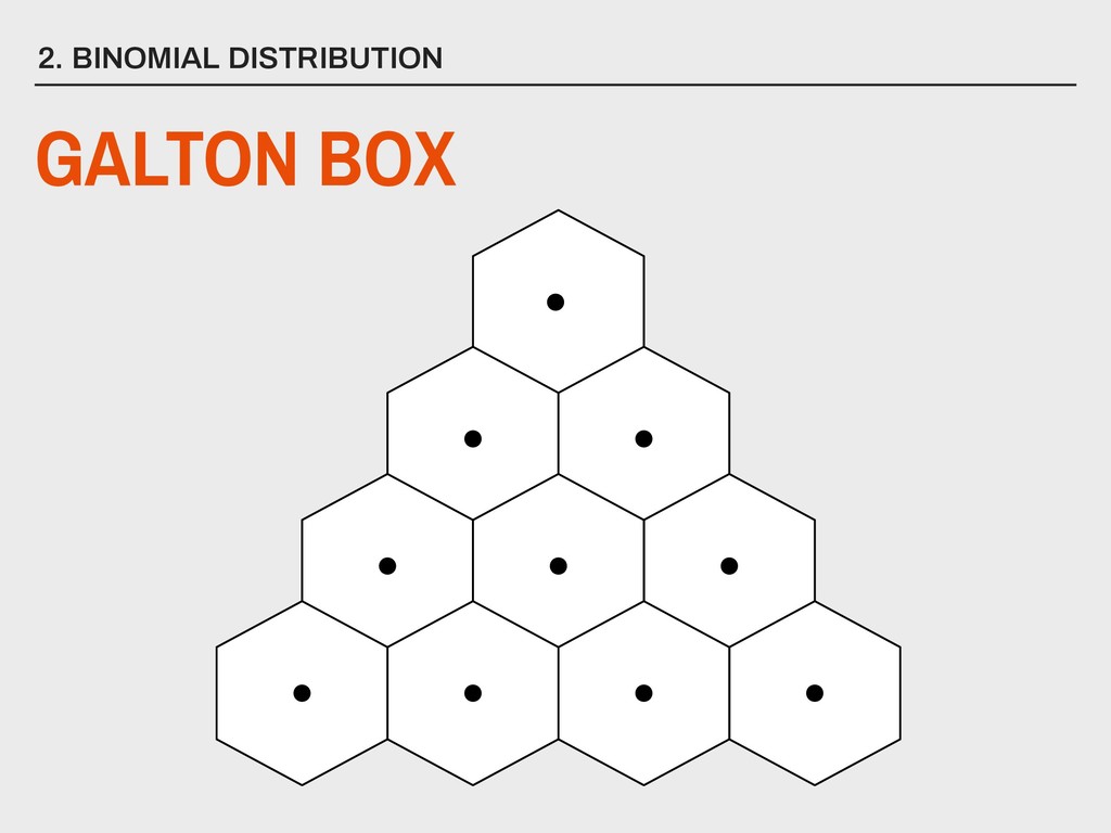
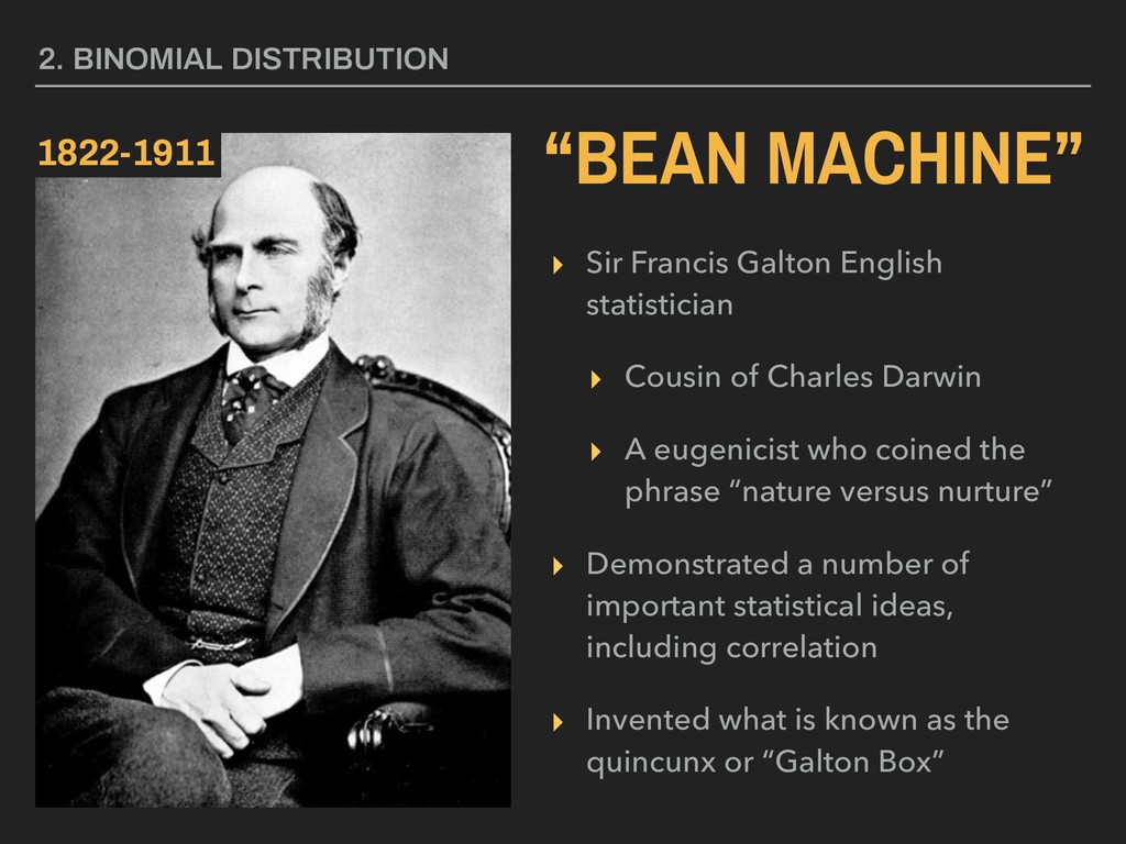
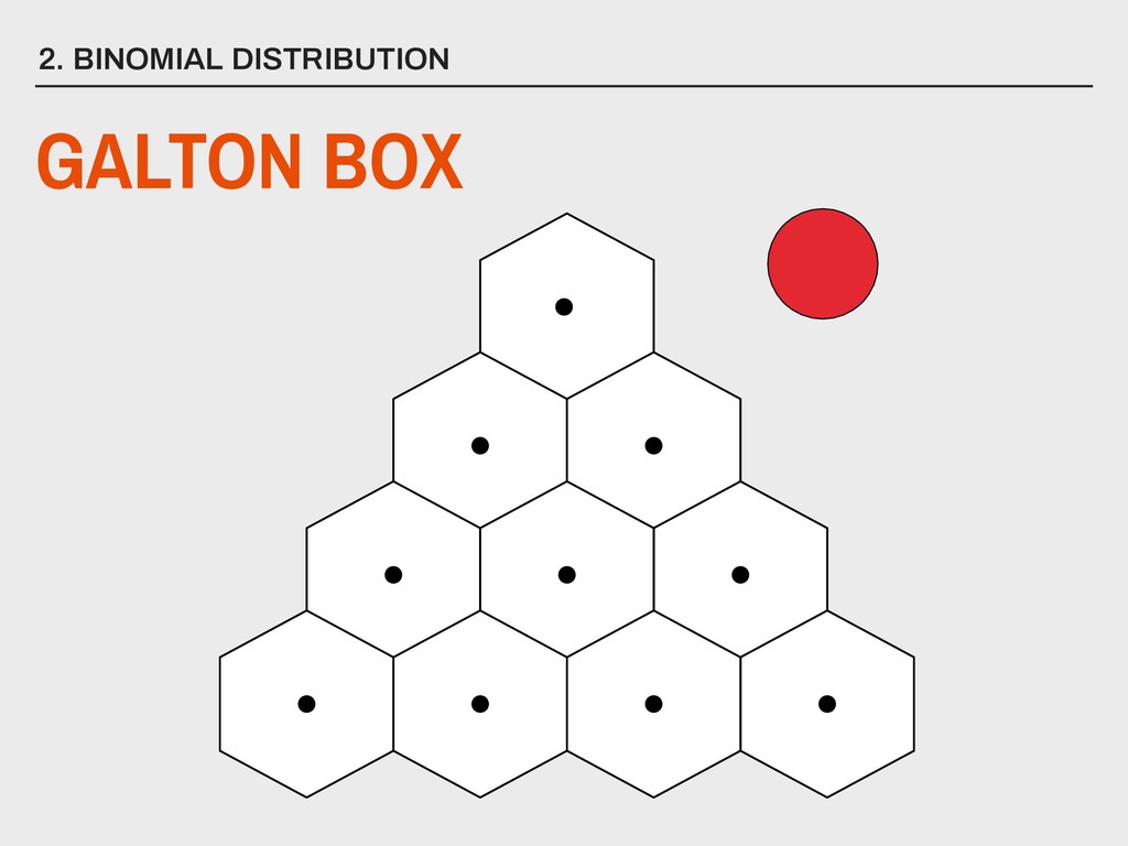
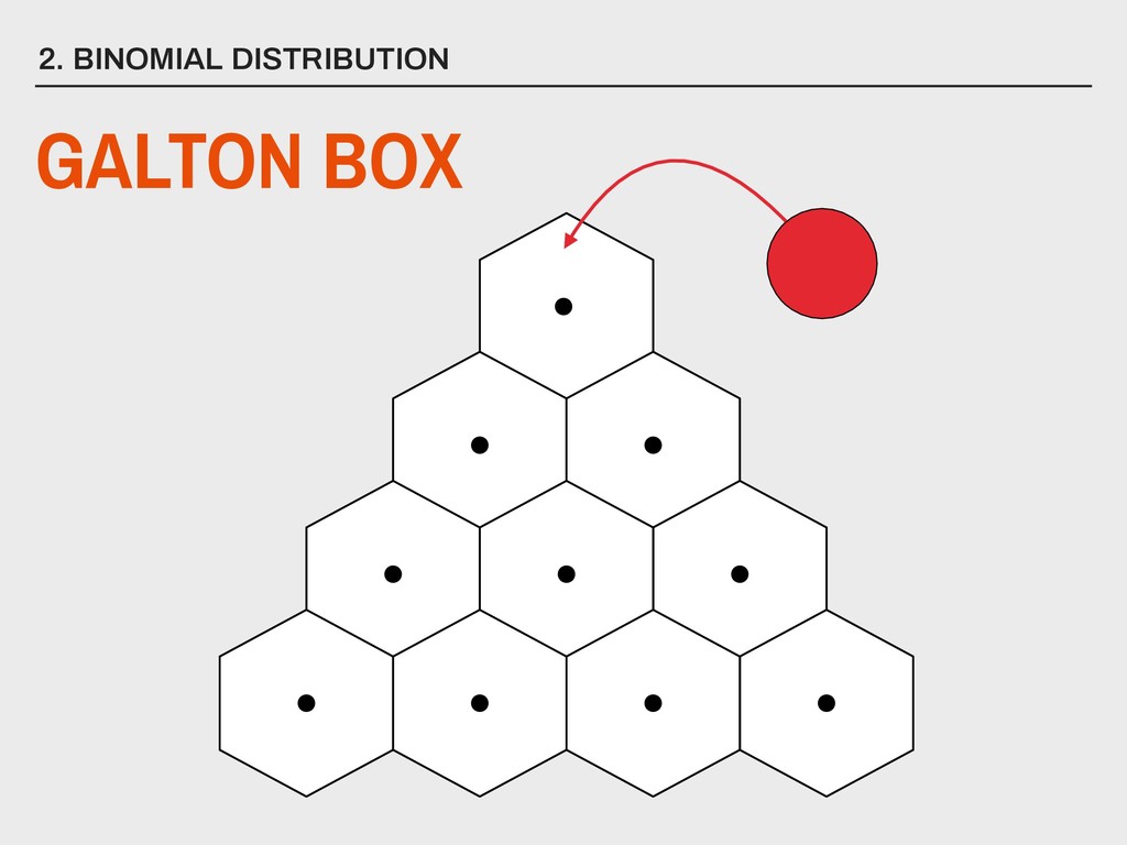
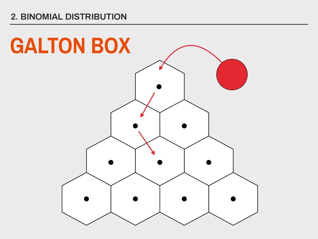
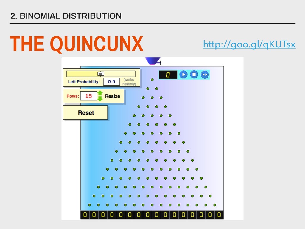
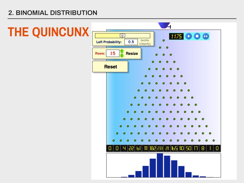
Darwin ▸ A eugenicist who coined the phrase “nature versus nurture” ▸ Demonstrated a number of important statistical ideas, including correlation ▸ Invented what is known as the quincunx or “Galton Box” 2. BINOMIAL DISTRIBUTION “BEAN MACHINE” 1822-1911
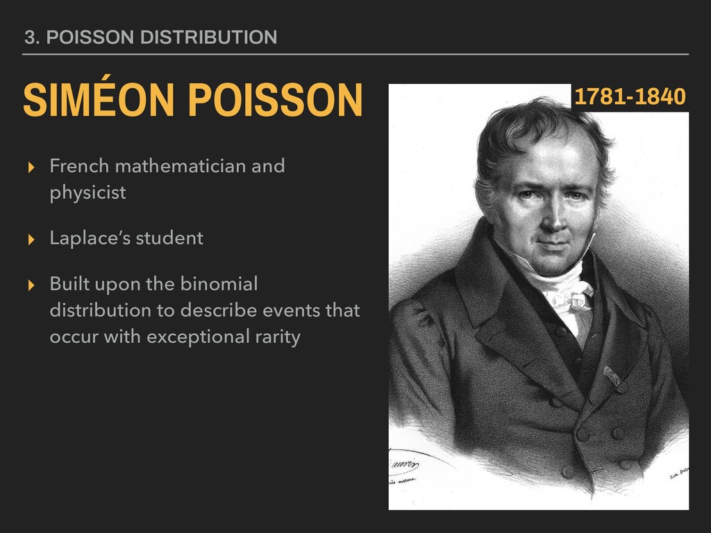
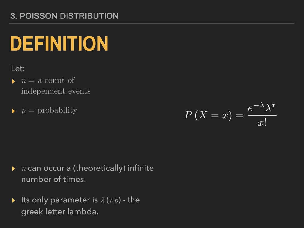
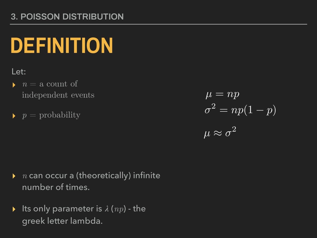
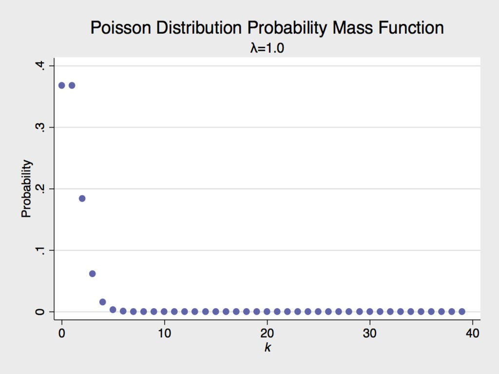
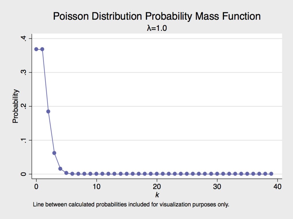
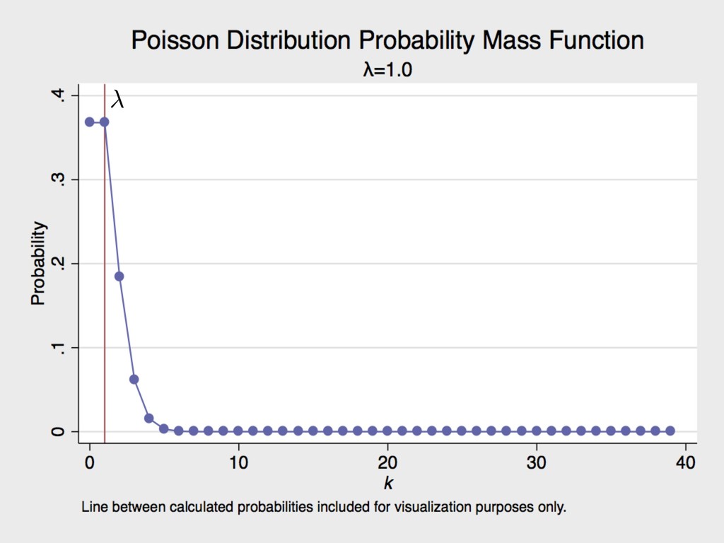
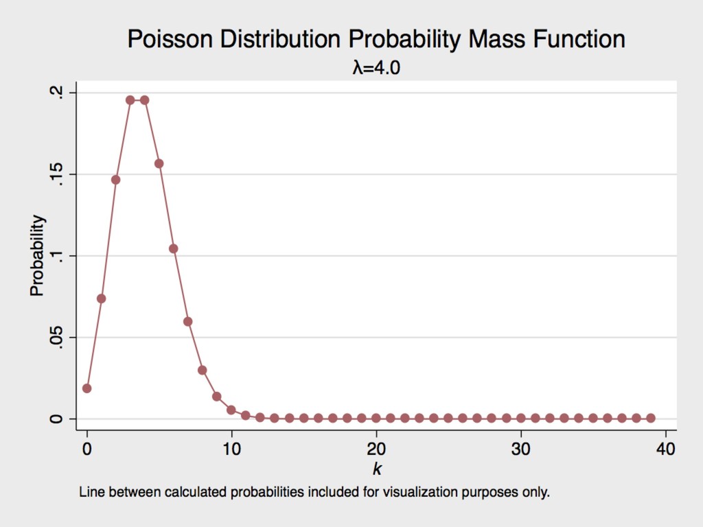
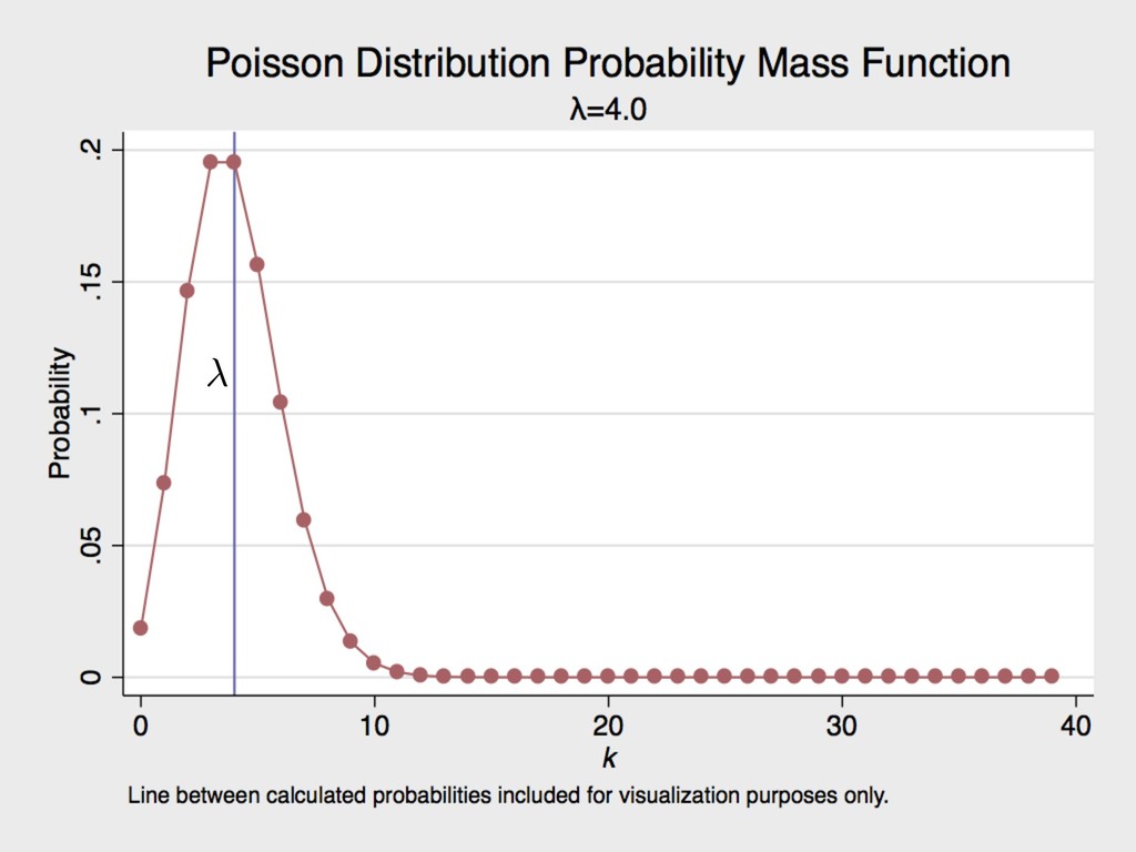
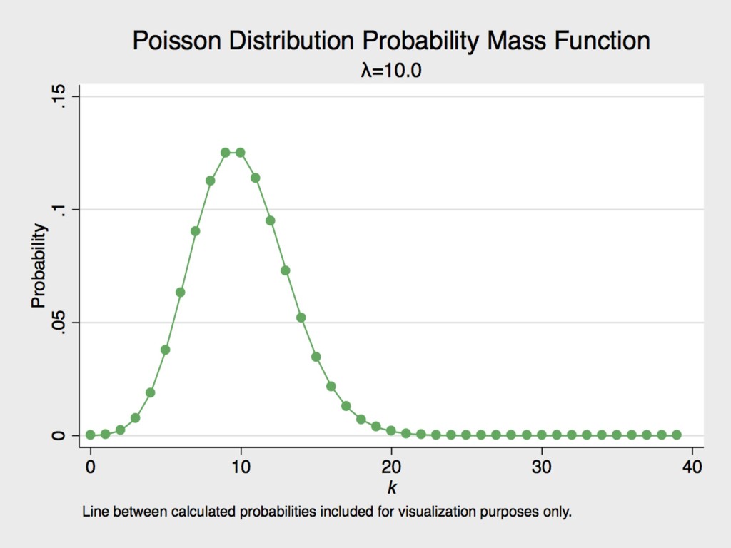
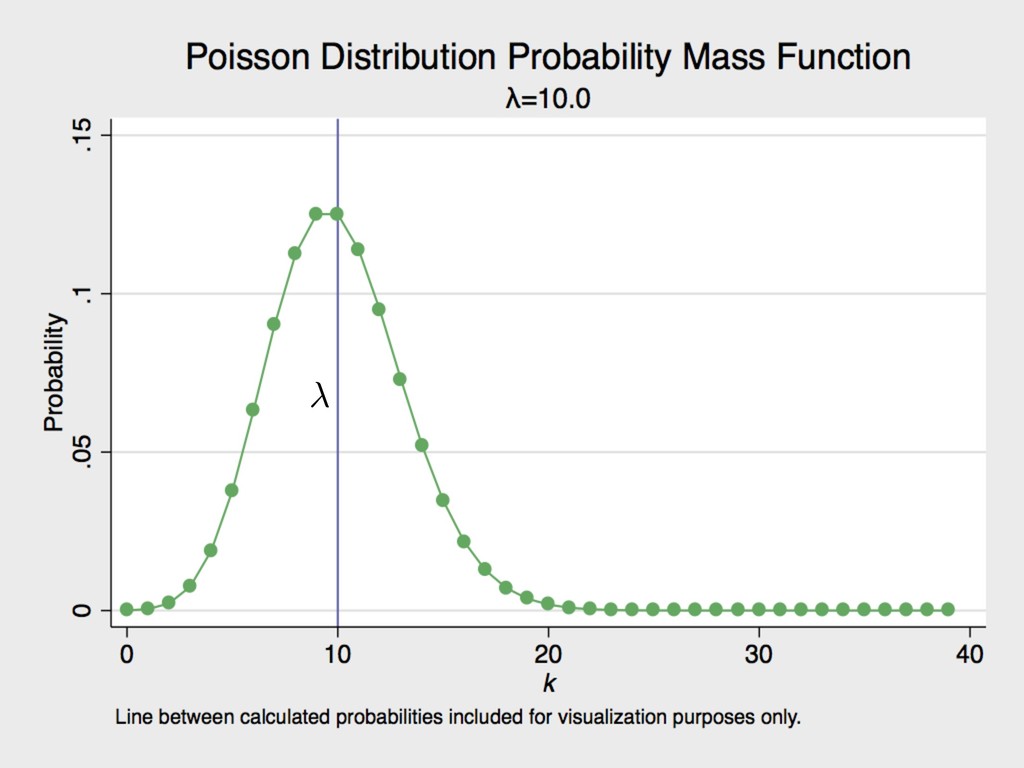
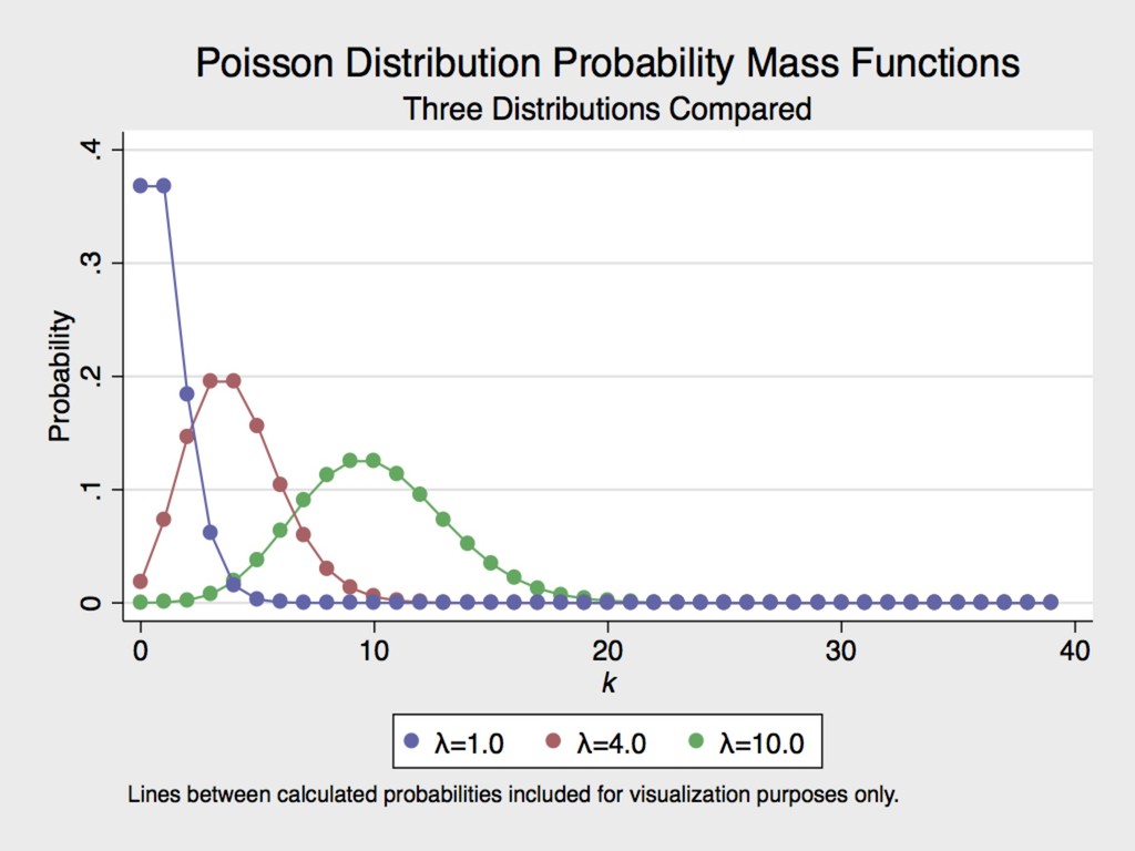
= probability 3. POISSON DISTRIBUTION Let: DEFINITION ▸ n can occur a (theoretically) infinite number of times. ▸ Its only parameter is (np) - the greek letter lambda.
= probability 3. POISSON DISTRIBUTION Let: DEFINITION ▸ n can occur a (theoretically) infinite number of times. ▸ Its only parameter is (np) - the greek letter lambda.
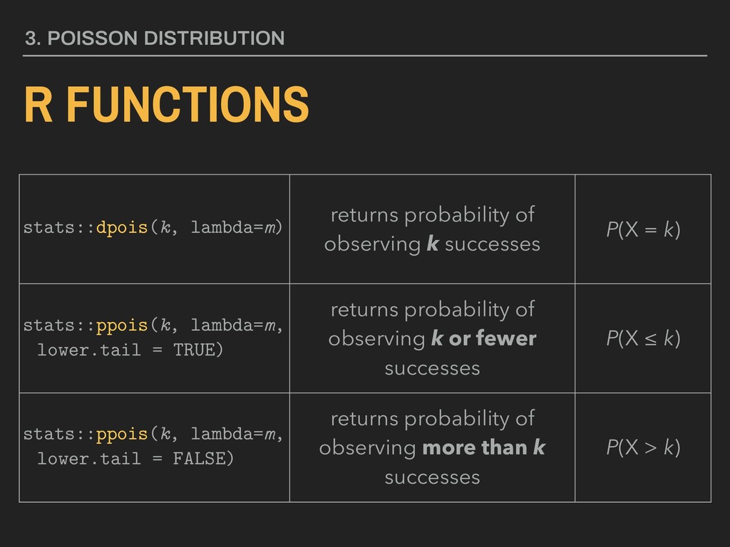
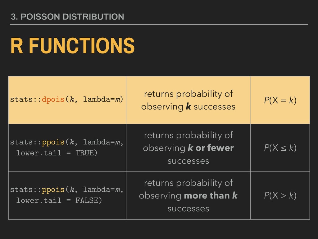
observing k successes P(X = k) stats::ppois(k, lambda=m, lower.tail = TRUE) returns probability of observing k or fewer successes P(X ≤ k) stats::ppois(k, lambda=m, lower.tail = FALSE) returns probability of observing more than k successes P(X > k)
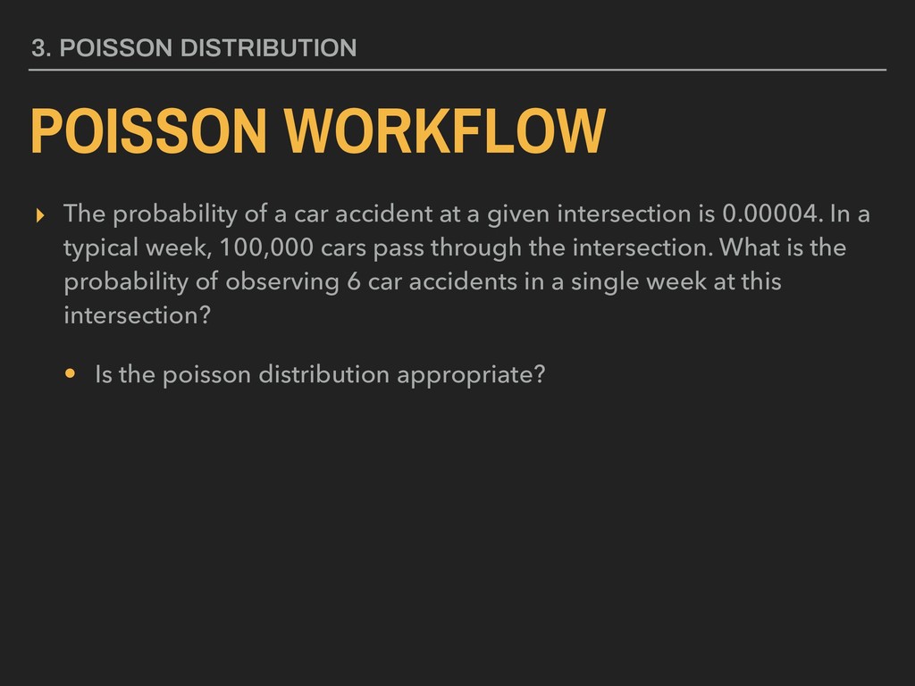
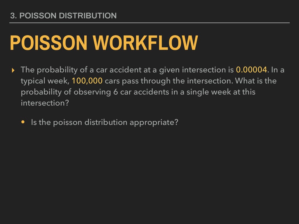
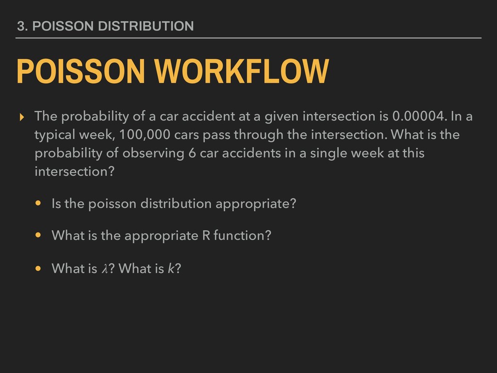
a given intersection is 0.00004. In a typical week, 100,000 cars pass through the intersection. What is the probability of observing 6 car accidents in a single week at this intersection? • Is the poisson distribution appropriate? 3. POISSON DISTRIBUTION
a given intersection is 0.00004. In a typical week, 100,000 cars pass through the intersection. What is the probability of observing 6 car accidents in a single week at this intersection? • Is the poisson distribution appropriate? 3. POISSON DISTRIBUTION
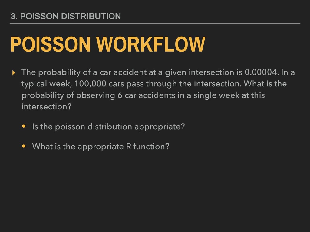
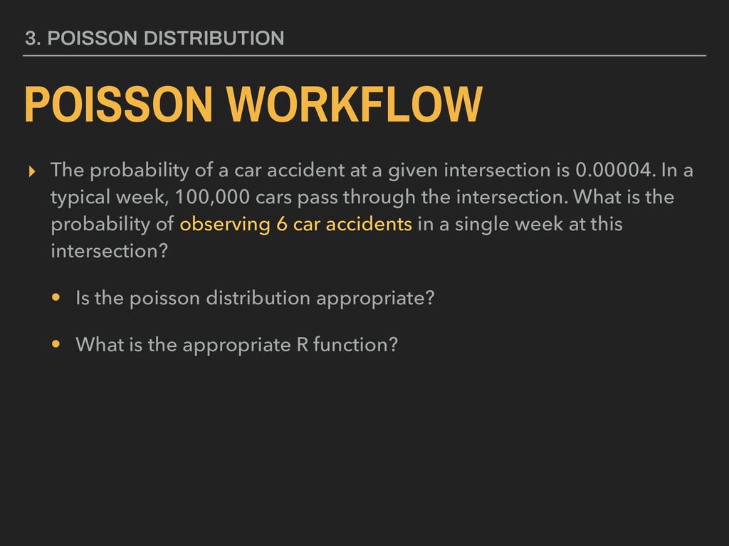
a given intersection is 0.00004. In a typical week, 100,000 cars pass through the intersection. What is the probability of observing 6 car accidents in a single week at this intersection? • Is the poisson distribution appropriate? • What is the appropriate R function? 3. POISSON DISTRIBUTION
a given intersection is 0.00004. In a typical week, 100,000 cars pass through the intersection. What is the probability of observing 6 car accidents in a single week at this intersection? • Is the poisson distribution appropriate? • What is the appropriate R function? 3. POISSON DISTRIBUTION
observing k successes P(X = k) stats::ppois(k, lambda=m, lower.tail = TRUE) returns probability of observing k or fewer successes P(X ≤ k) stats::ppois(k, lambda=m, lower.tail = FALSE) returns probability of observing more than k successes P(X > k)
observing k successes P(X = k) stats::ppois(k, lambda=m, lower.tail = TRUE) returns probability of observing k or fewer successes P(X ≤ k) stats::ppois(k, lambda=m, lower.tail = FALSE) returns probability of observing more than k successes P(X > k)
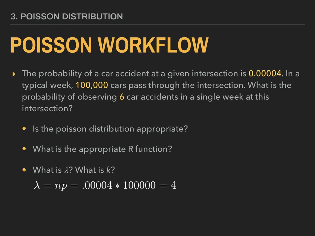
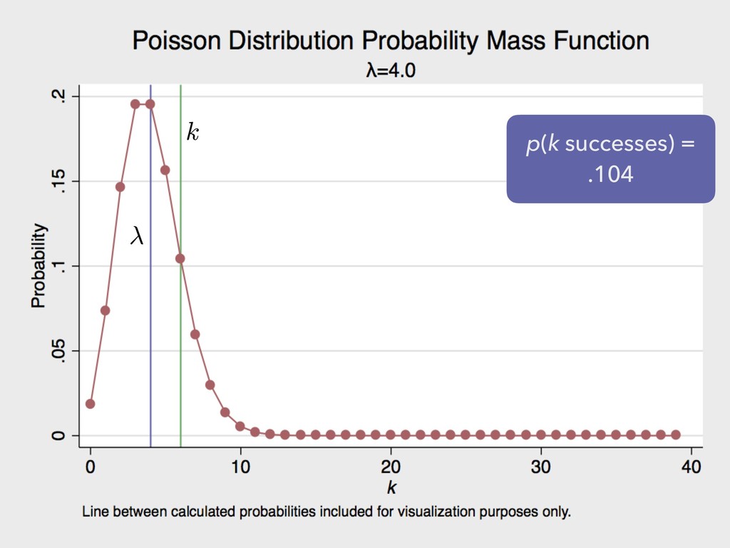
a given intersection is 0.00004. In a typical week, 100,000 cars pass through the intersection. What is the probability of observing 6 car accidents in a single week at this intersection? • Is the poisson distribution appropriate? • What is the appropriate R function? • What is ? What is k? 3. POISSON DISTRIBUTION
a given intersection is 0.00004. In a typical week, 100,000 cars pass through the intersection. What is the probability of observing 6 car accidents in a single week at this intersection? • Is the poisson distribution appropriate? • What is the appropriate R function? • What is ? What is k? 3. POISSON DISTRIBUTION
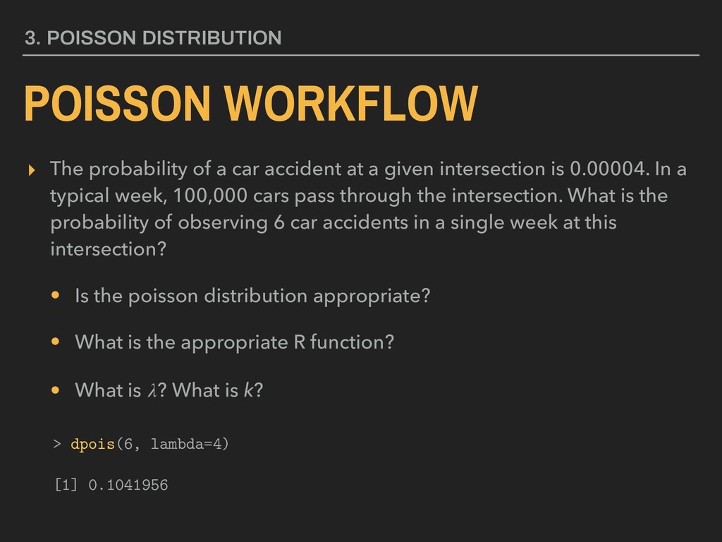
a given intersection is 0.00004. In a typical week, 100,000 cars pass through the intersection. What is the probability of observing 6 car accidents in a single week at this intersection? • Is the poisson distribution appropriate? • What is the appropriate R function? • What is ? What is k? 3. POISSON DISTRIBUTION > dpois(6, lambda=4) [1] 0.1041956
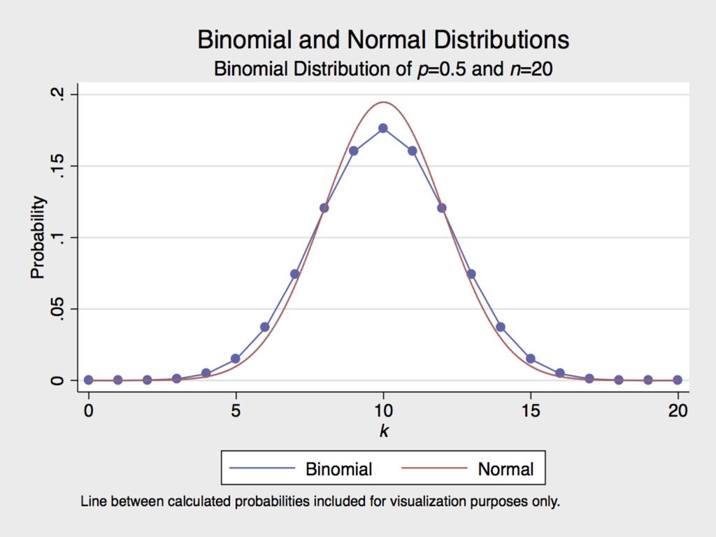
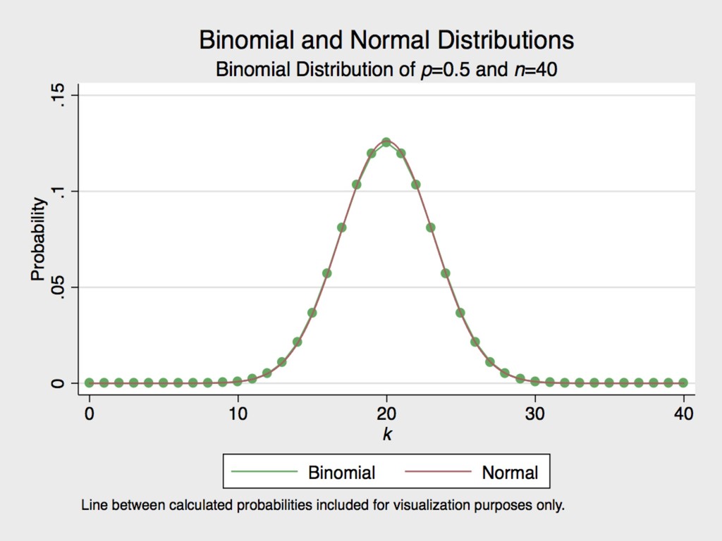
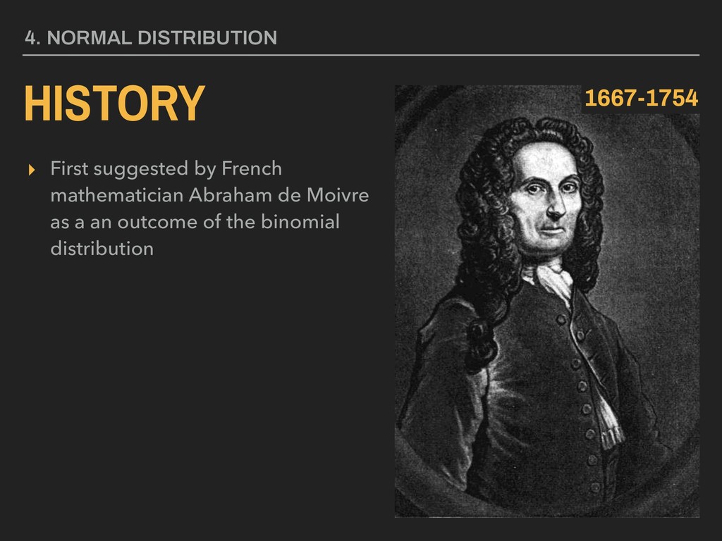
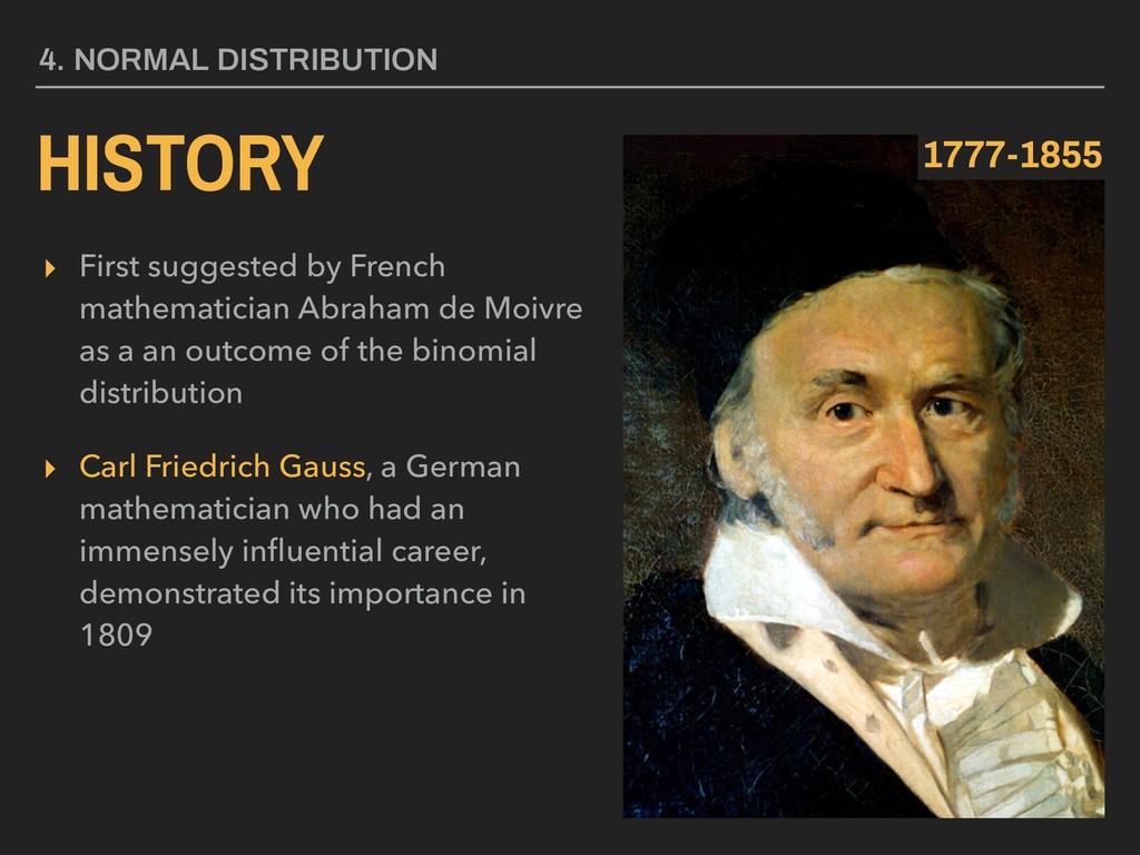
a an outcome of the binomial distribution ▸ Carl Friedrich Gauss, a German mathematician who had an immensely influential career, demonstrated its importance in 1809 4. NORMAL DISTRIBUTION HISTORY 1777-1855
a an outcome of the binomial distribution ▸ Carl Friedrich Gauss, a German mathematician who had an immensely influential career, demonstrated its importance in 1809 ▸ Pierre Simon Laplace also made significant contributions to its usefulness beginning in 1810 4. NORMAL DISTRIBUTION HISTORY 1749-1827
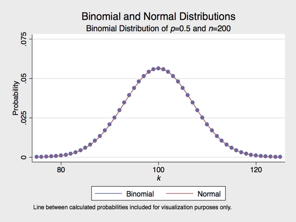
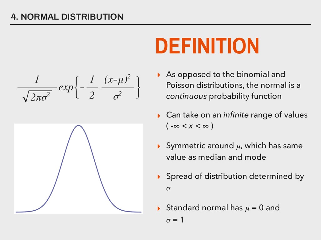
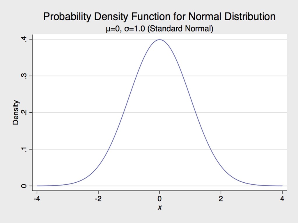
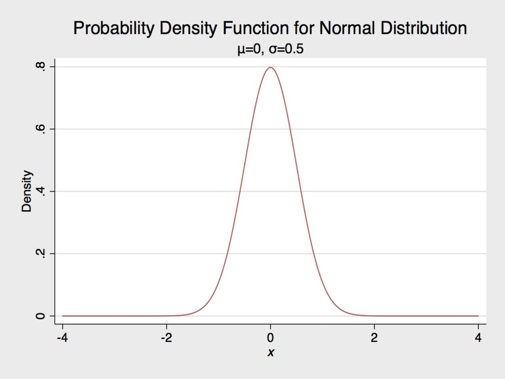
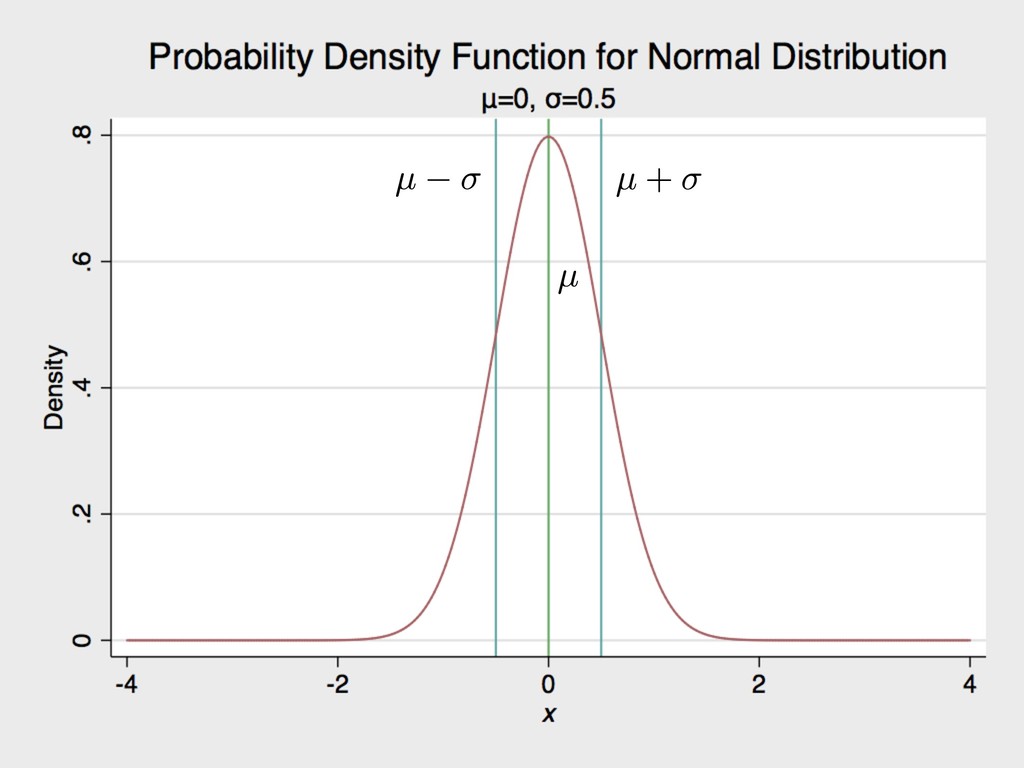
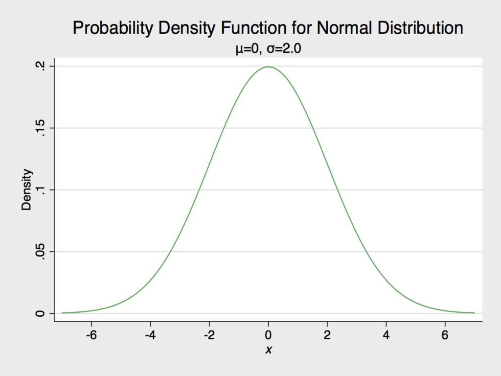
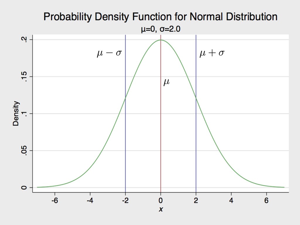
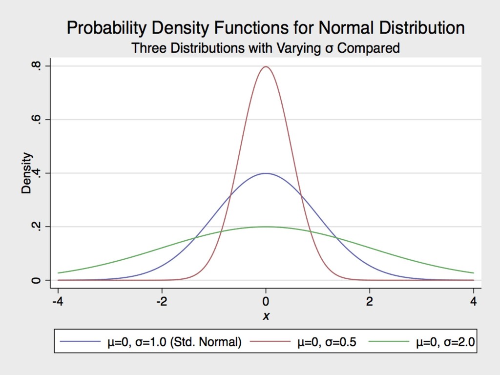
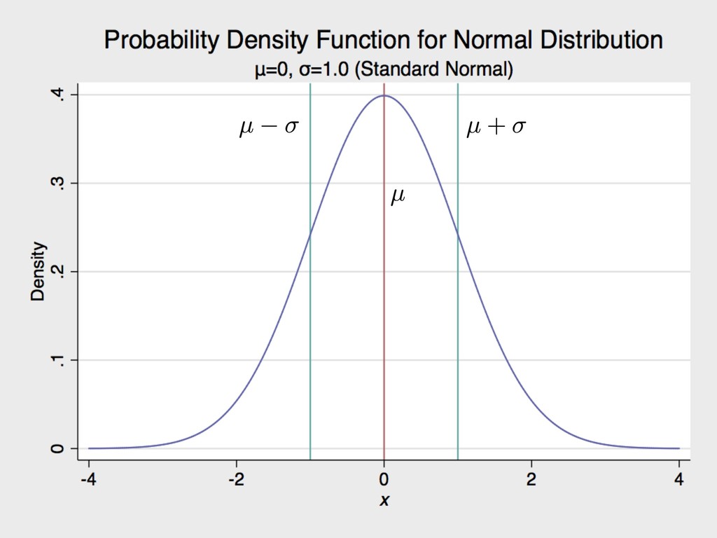
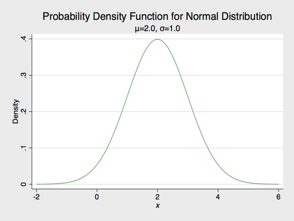
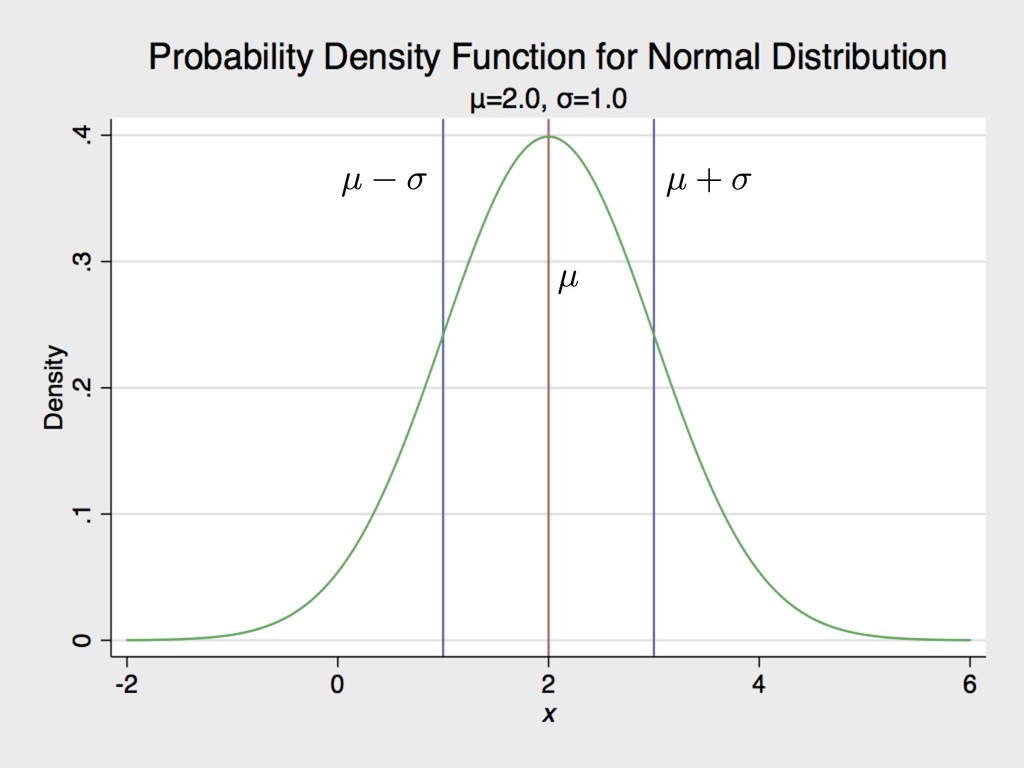
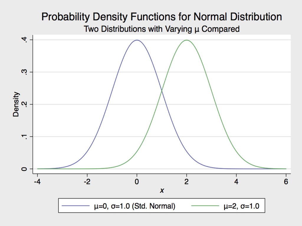
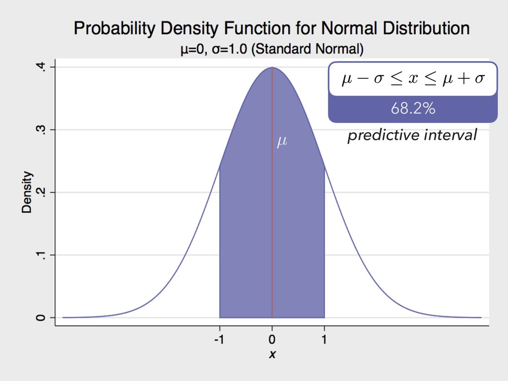
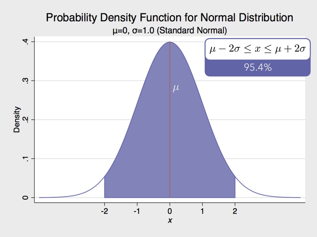
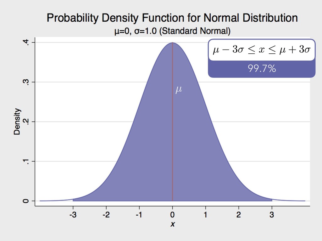
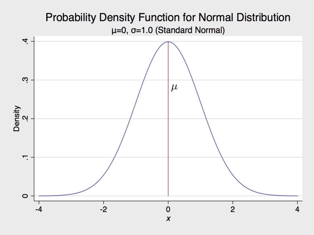
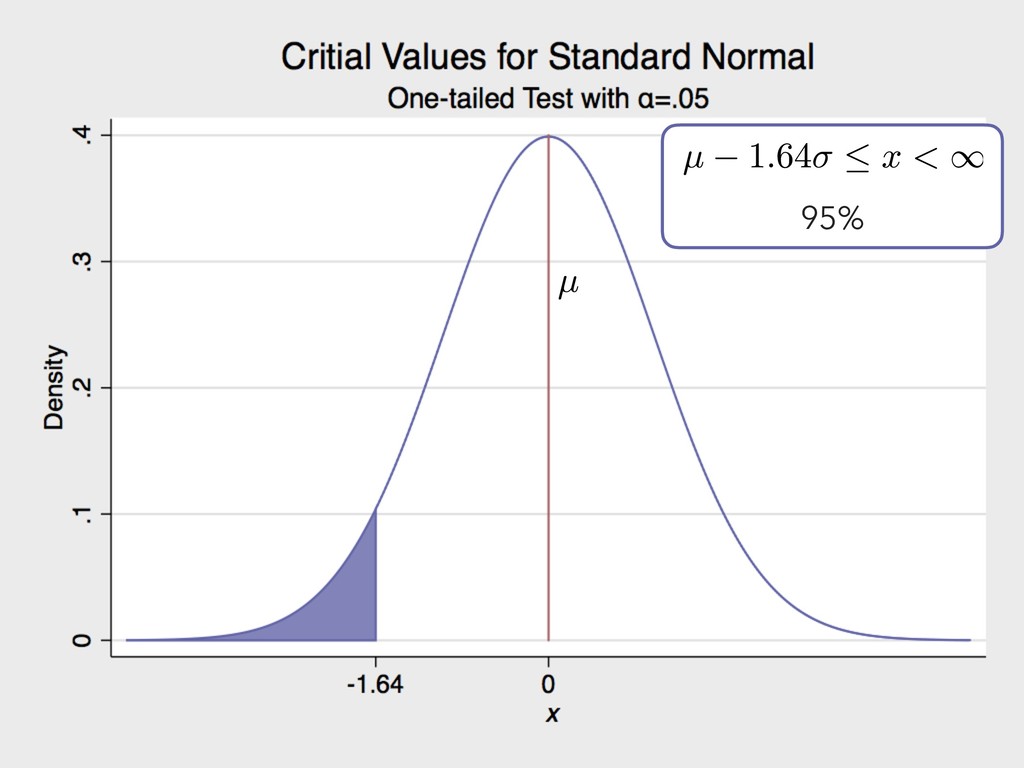
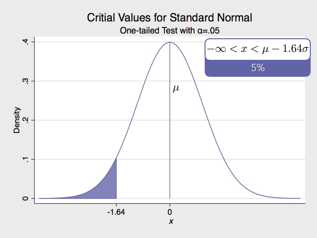
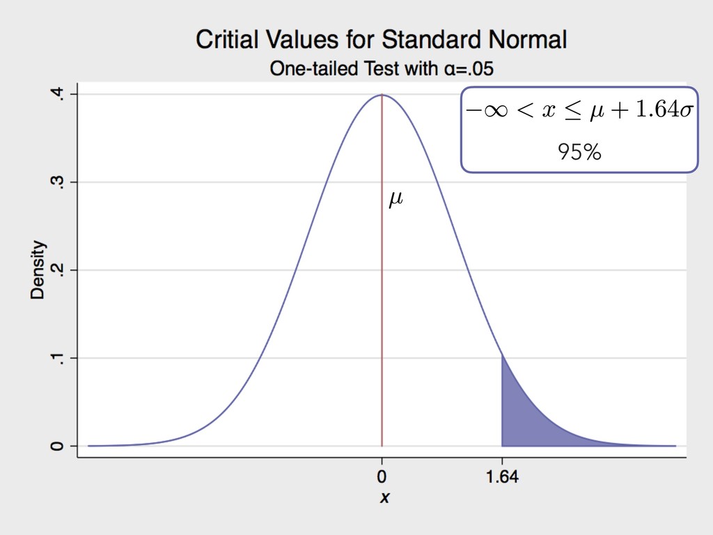
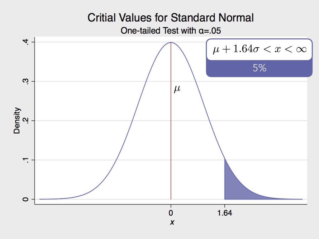
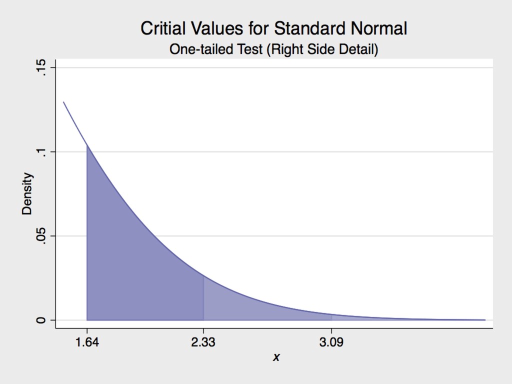
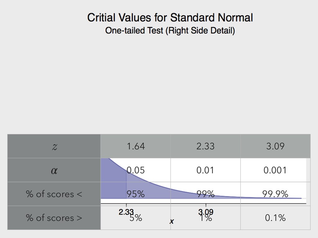
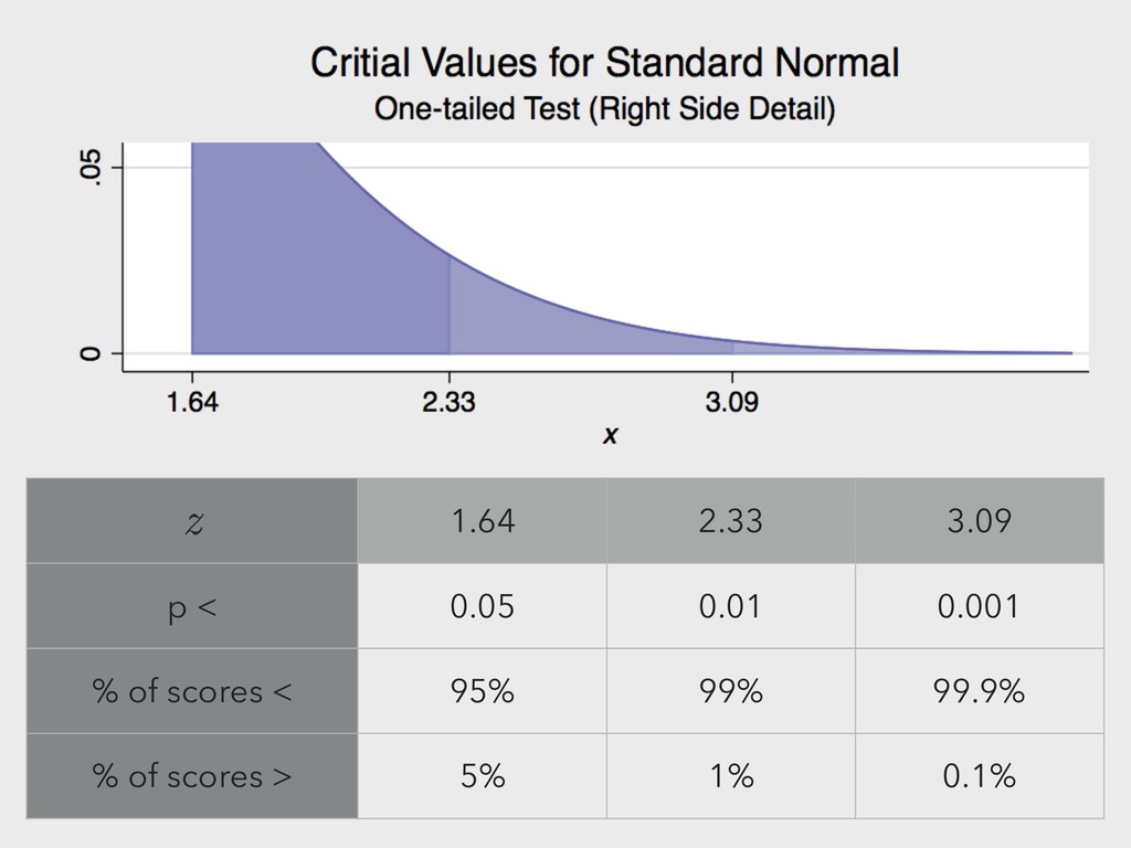
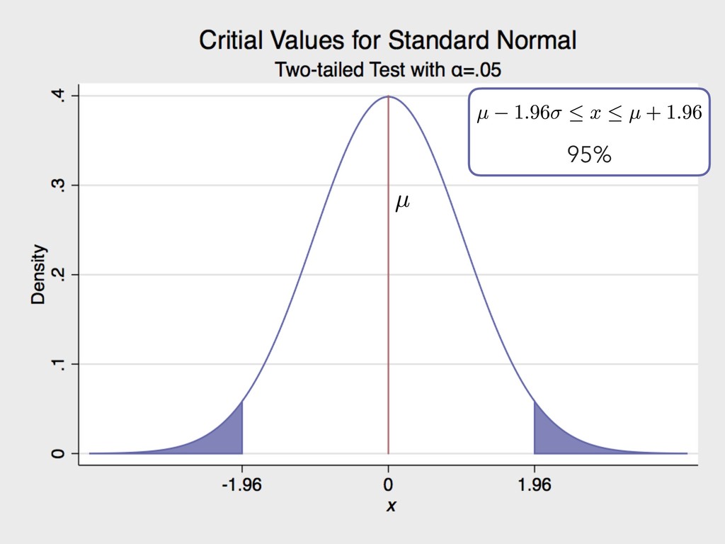
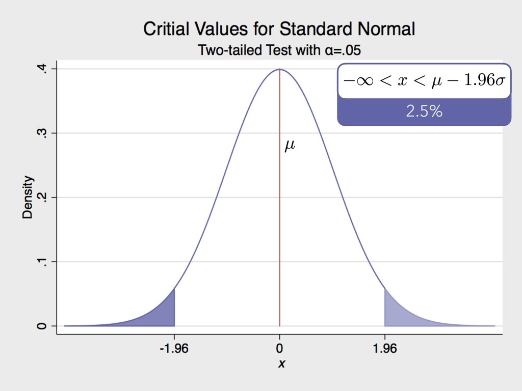
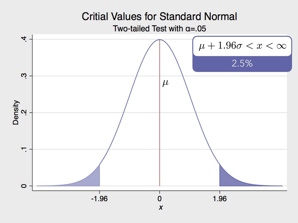
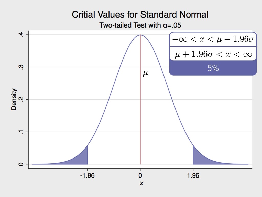
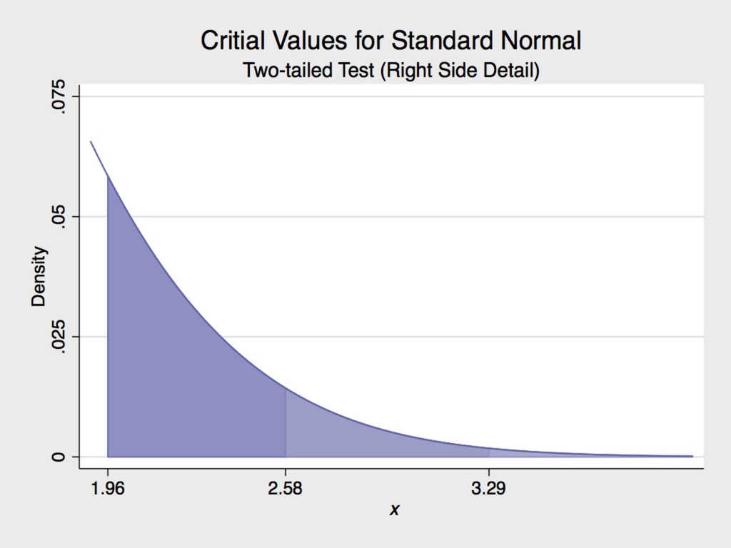
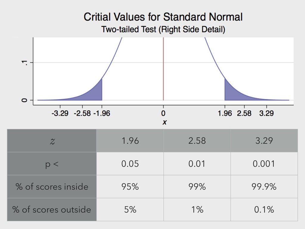
normal is a continuous probability function ▸ Can take on an infinite range of values ( -∞ < x < ∞ ) ▸ Symmetric around , which has same value as median and mode ▸ Spread of distribution determined by ▸ Standard normal has = 0 and = 1 4. NORMAL DISTRIBUTION DEFINITION
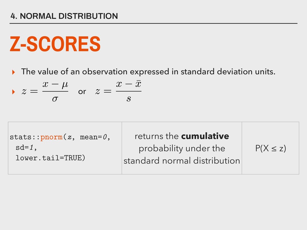
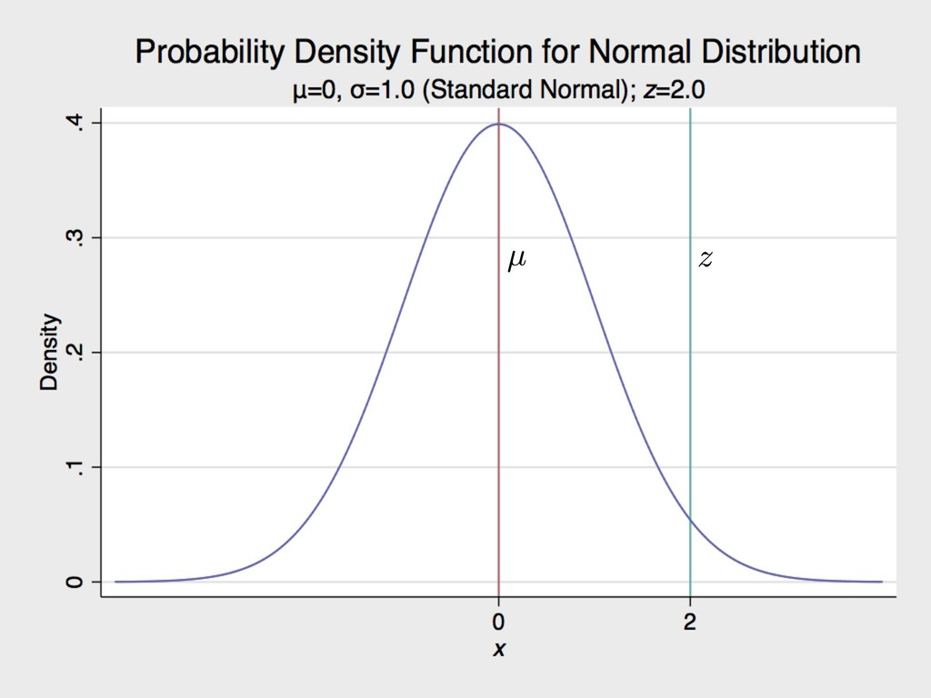
expressed in standard deviation units. ▸ or stats::pnorm(z, mean=0, sd=1, lower.tail=TRUE) returns the cumulative probability under the standard normal distribution P(X ≤ z)
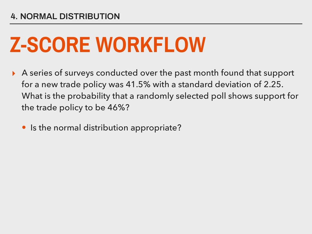
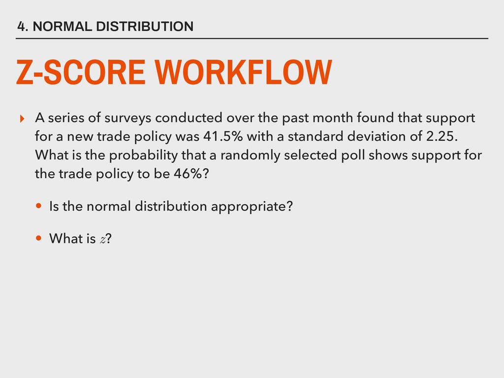
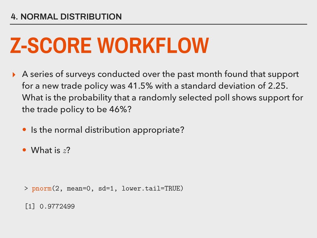
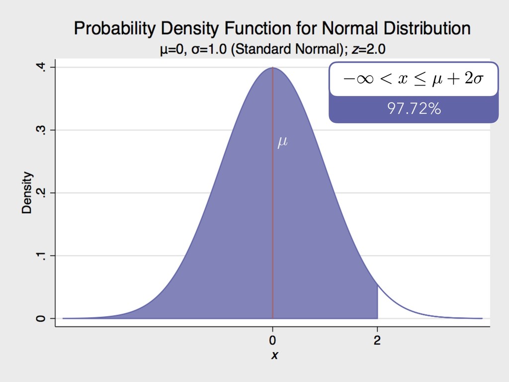
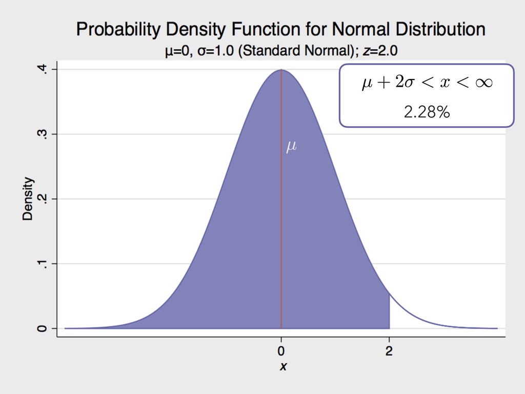
found that support for a new trade policy was 41.5% with a standard deviation of 2.25. What is the probability that a randomly selected poll shows support for the trade policy to be 46%? • Is the normal distribution appropriate? 4. NORMAL DISTRIBUTION Z-SCORE WORKFLOW
found that support for a new trade policy was 41.5% with a standard deviation of 2.25. What is the probability that a randomly selected poll shows support for the trade policy to be 46%? • Is the normal distribution appropriate? • What is z? 4. NORMAL DISTRIBUTION Z-SCORE WORKFLOW
found that support for a new trade policy was 41.5% with a standard deviation of 2.25. What is the probability that a randomly selected poll shows support for the trade policy to be 46%? • Is the normal distribution appropriate? • What is z? 4. NORMAL DISTRIBUTION Z-SCORE WORKFLOW
found that support for a new trade policy was 41.5% with a standard deviation of 2.25. What is the probability that a randomly selected poll shows support for the trade policy to be 46%? • Is the normal distribution appropriate? • What is z? 4. NORMAL DISTRIBUTION Z-SCORE WORKFLOW > pnorm(2, mean=0, sd=1, lower.tail=TRUE) [1] 0.9772499
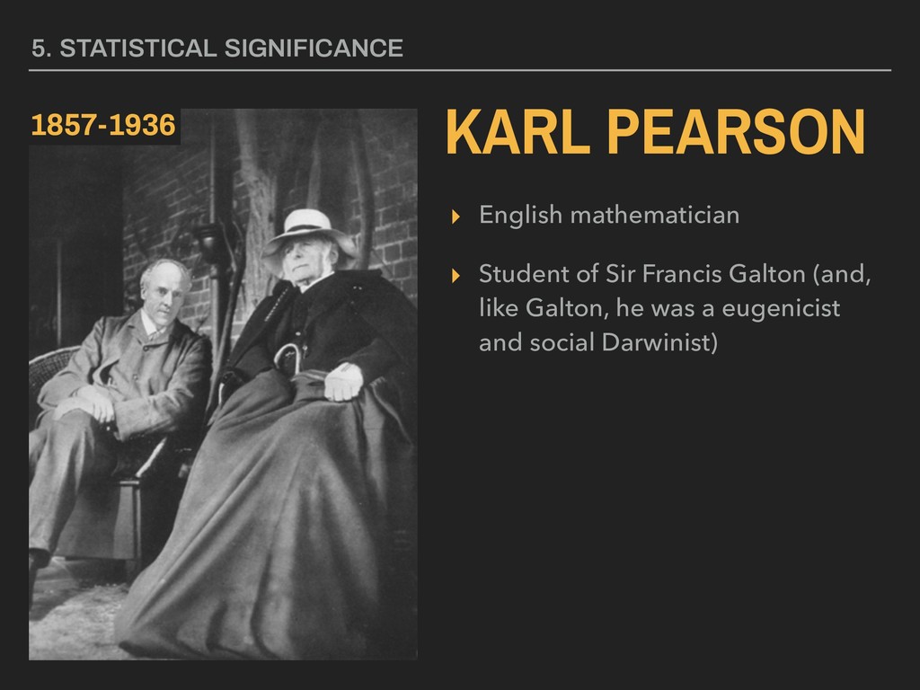
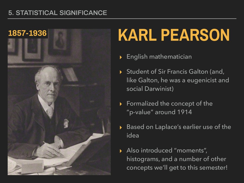
like Galton, he was a eugenicist and social Darwinist) ▸ Formalized the concept of the “p-value” around 1914 ▸ Based on Laplace’s earlier use of the idea ▸ Also introduced “moments”, histograms, and a number of other concepts we’ll get to this semester! 5. STATISTICAL SIGNIFICANCE KARL PEARSON 1857-1936
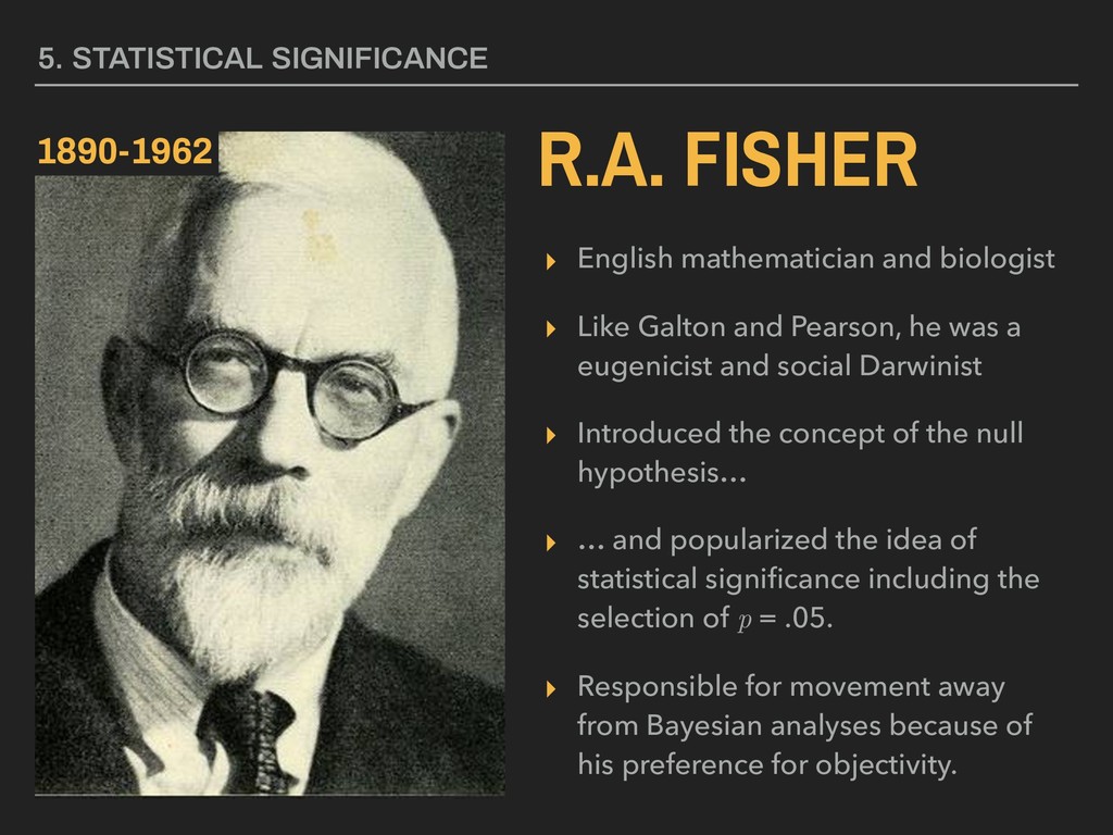
he was a eugenicist and social Darwinist ▸ Introduced the concept of the null hypothesis… ▸ … and popularized the idea of statistical significance including the selection of p = .05. ▸ Responsible for movement away from Bayesian analyses because of his preference for objectivity. 5. STATISTICAL SIGNIFICANCE R.A. FISHER 1890-1962
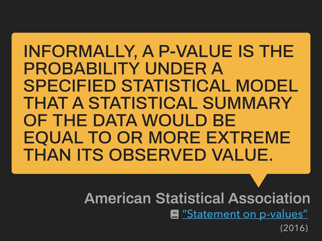
MODEL THAT A STATISTICAL SUMMARY OF THE DATA WOULD BE EQUAL TO OR MORE EXTREME THAN ITS OBSERVED VALUE. American Statistical Association “Statement on p-values” (2016)
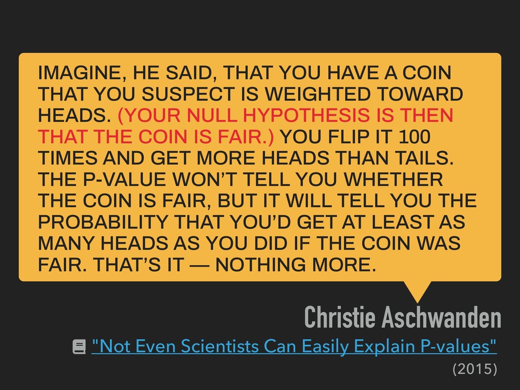
SUSPECT IS WEIGHTED TOWARD HEADS. (YOUR NULL HYPOTHESIS IS THEN THAT THE COIN IS FAIR.) YOU FLIP IT 100 TIMES AND GET MORE HEADS THAN TAILS. THE P-VALUE WON’T TELL YOU WHETHER THE COIN IS FAIR, BUT IT WILL TELL YOU THE PROBABILITY THAT YOU’D GET AT LEAST AS MANY HEADS AS YOU DID IF THE COIN WAS FAIR. THAT’S IT — NOTHING MORE. Christie Aschwanden "Not Even Scientists Can Easily Explain P-values" (2015)
P = 0.05? A: BECAUSE THAT’S STILL WHAT THE SCIENTIFIC COMMUNITY AND JOURNAL EDITORS USE. Q: WHY DO SO MANY PEOPLE STILL USE P = 0.05? A: BECAUSE THAT’S WHAT THEY WERE TAUGHT IN COLLEGE OR GRAD SCHOOL. George Cobb, Ph.D. “Statement on p-values” (2015)
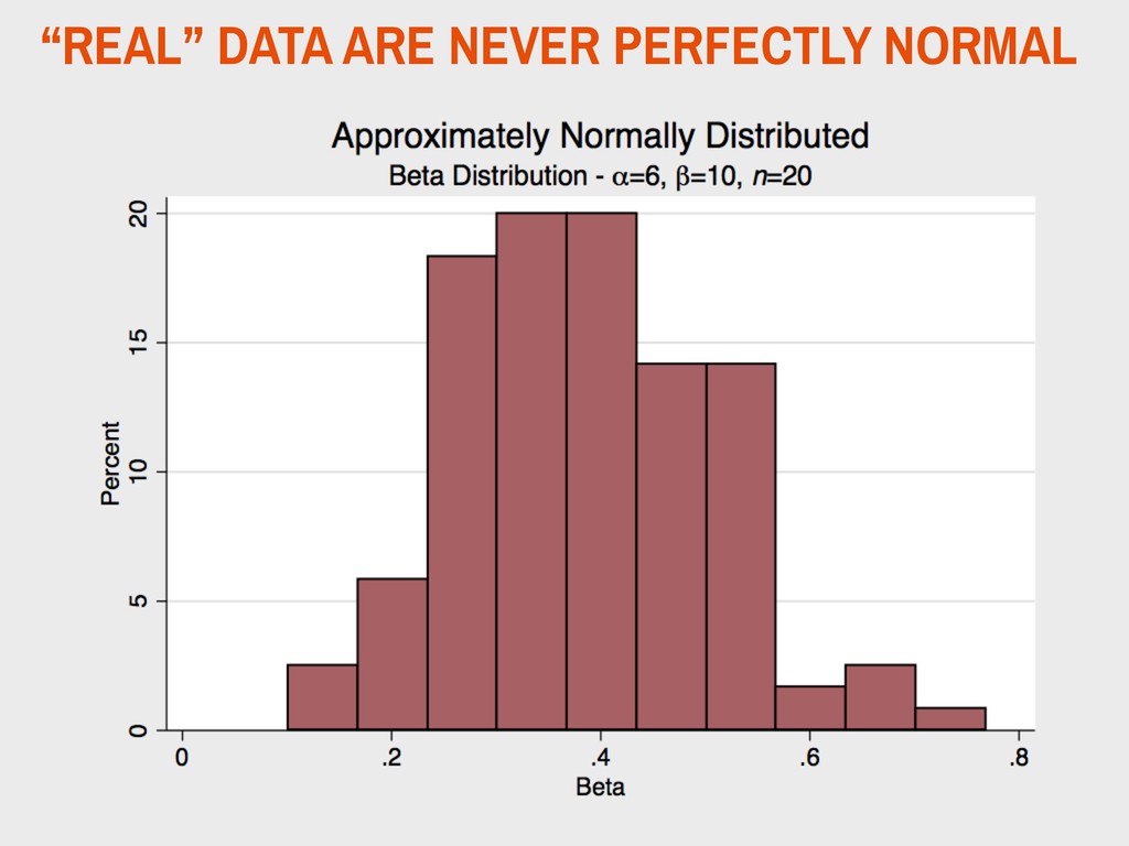
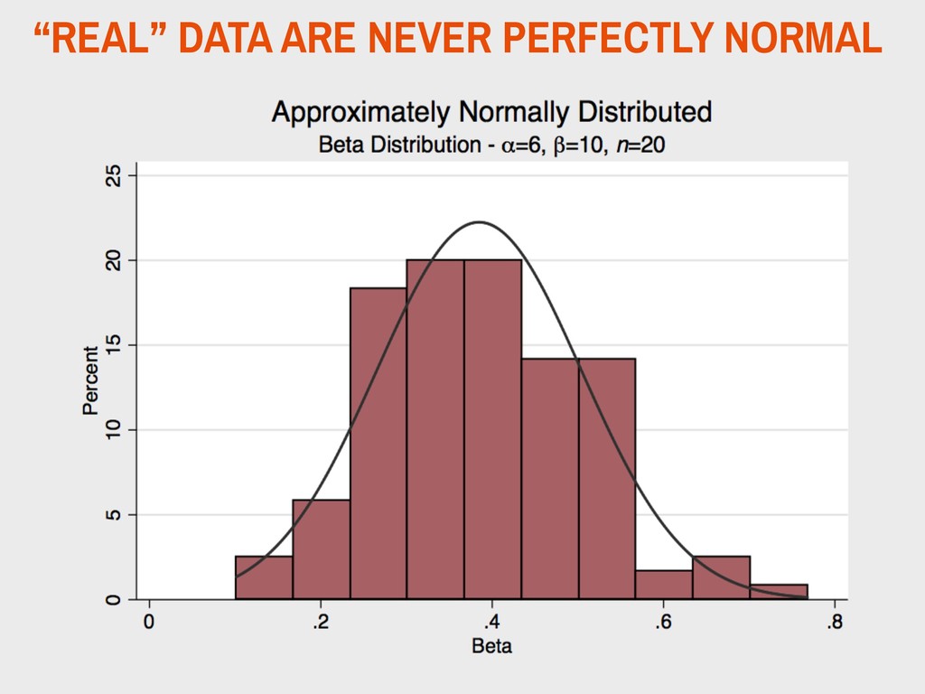
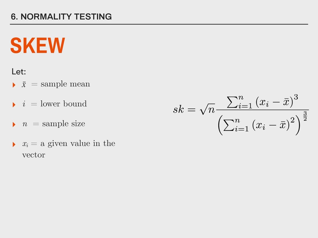
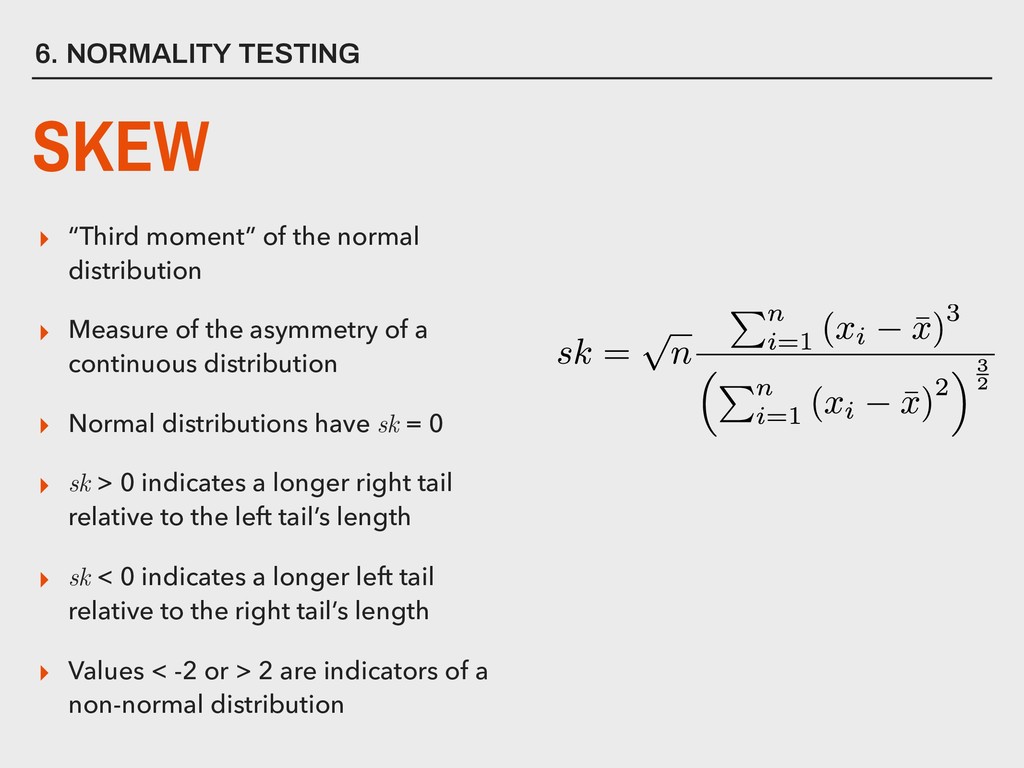
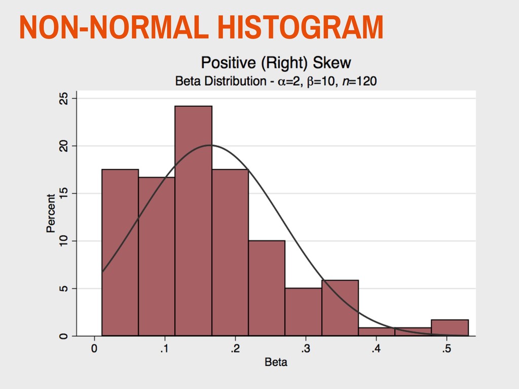
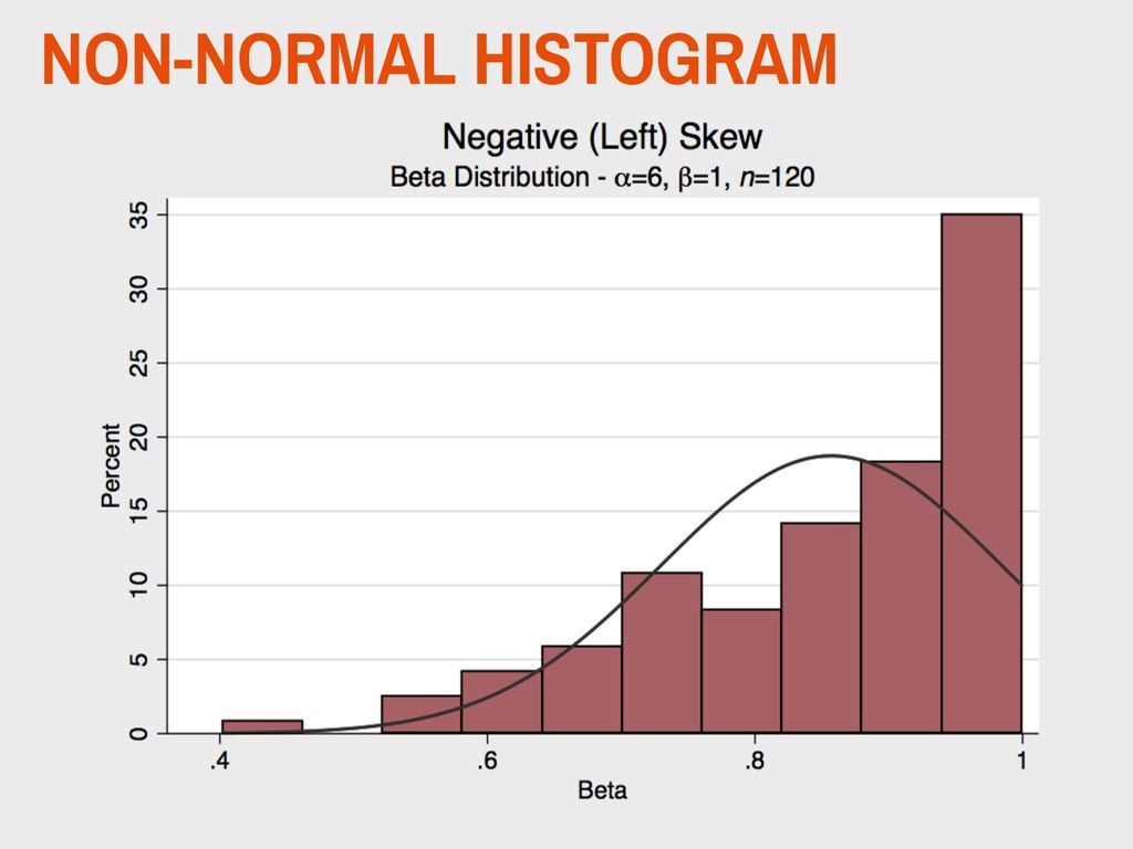
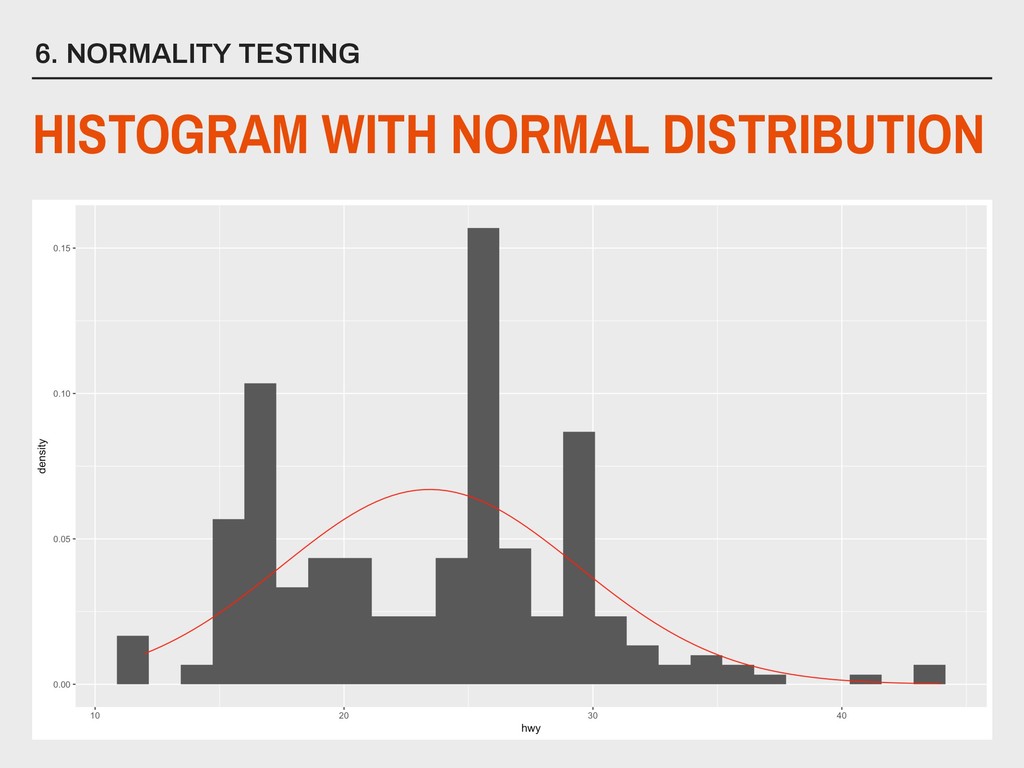
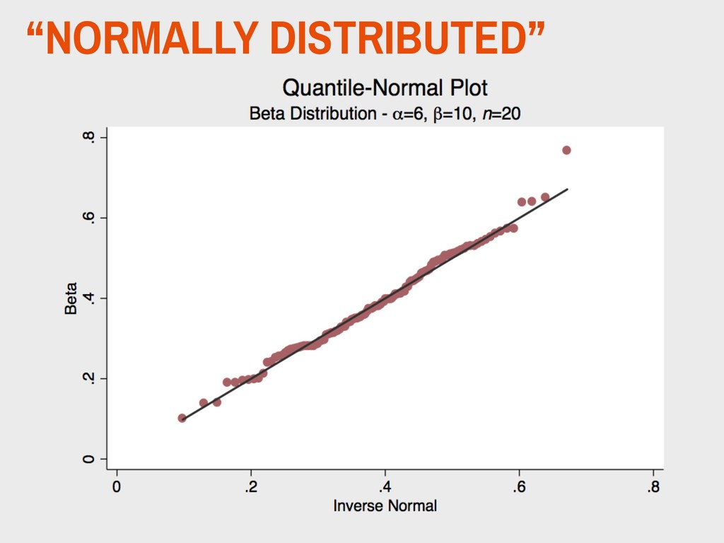
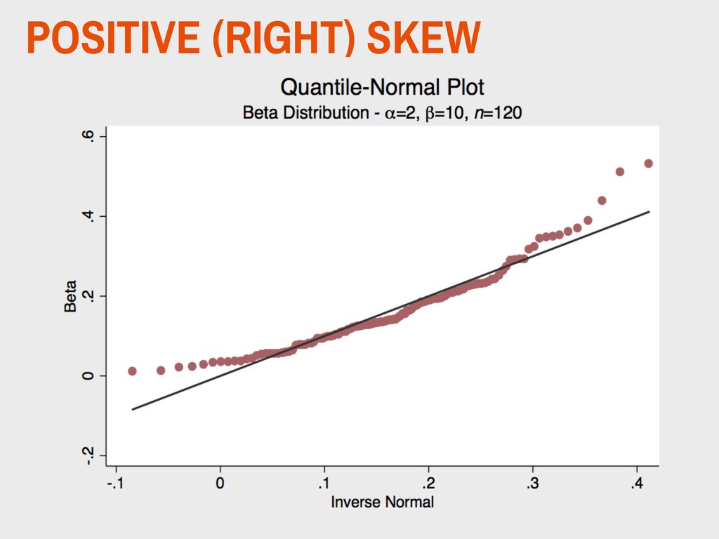
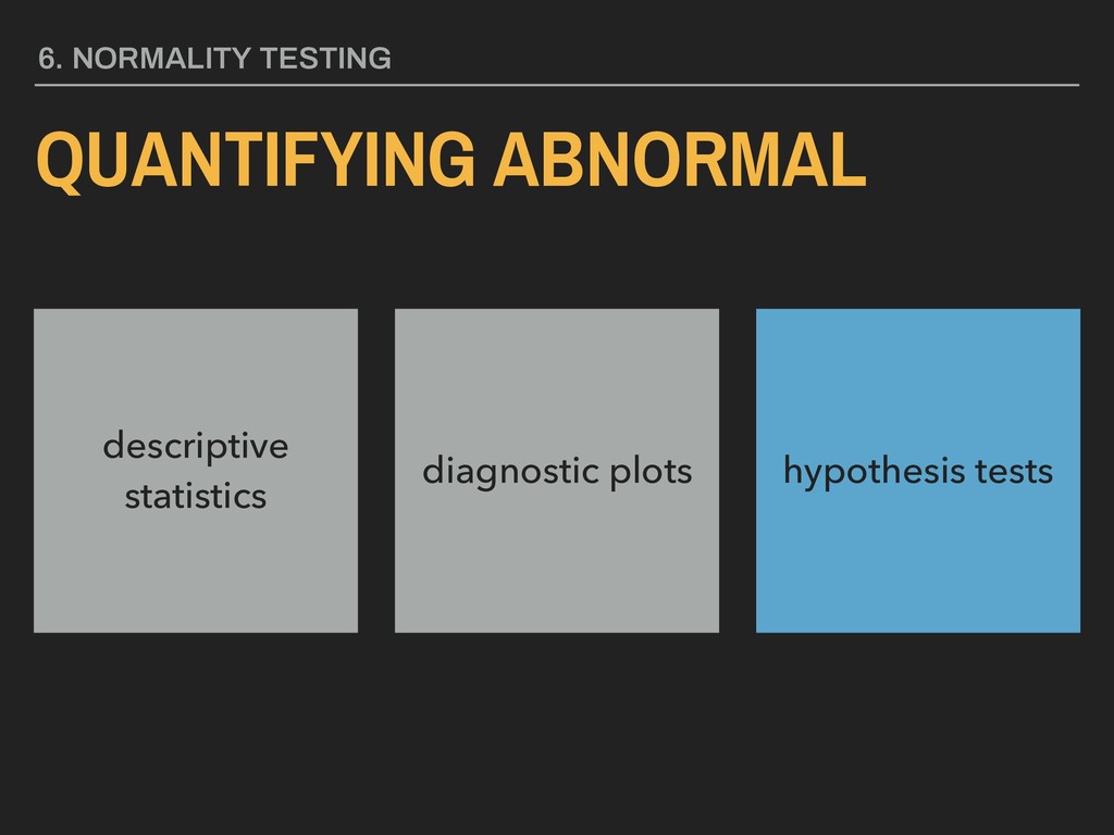
the asymmetry of a continuous distribution ▸ Normal distributions have sk = 0 ▸ sk > 0 indicates a longer right tail relative to the left tail’s length ▸ sk < 0 indicates a longer left tail relative to the right tail’s length ▸ Values < -2 or > 2 are indicators of a non-normal distribution 6. NORMALITY TESTING SKEW
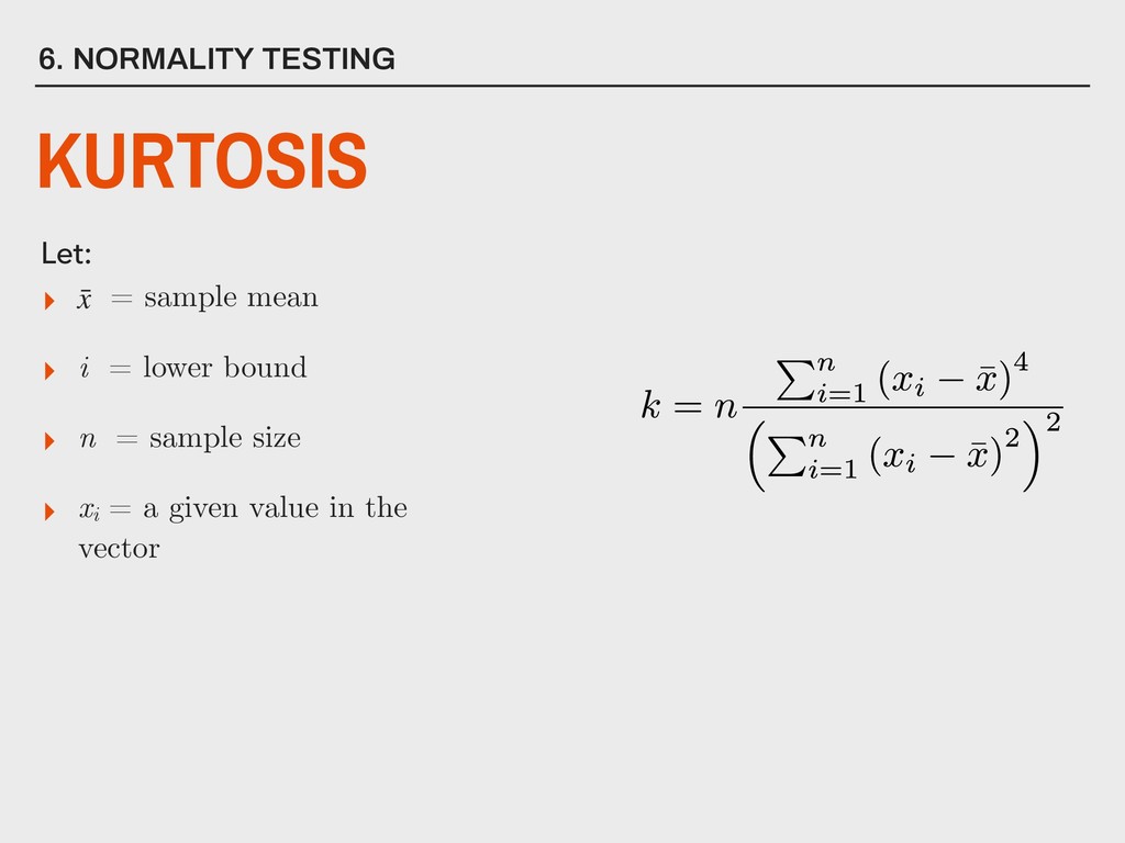
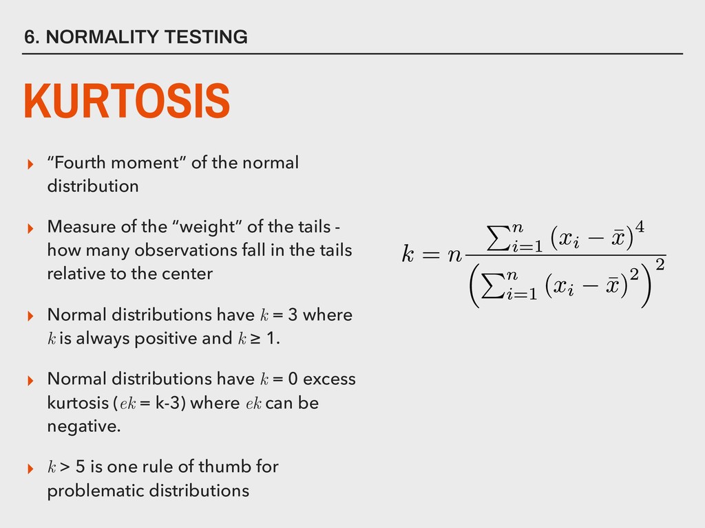
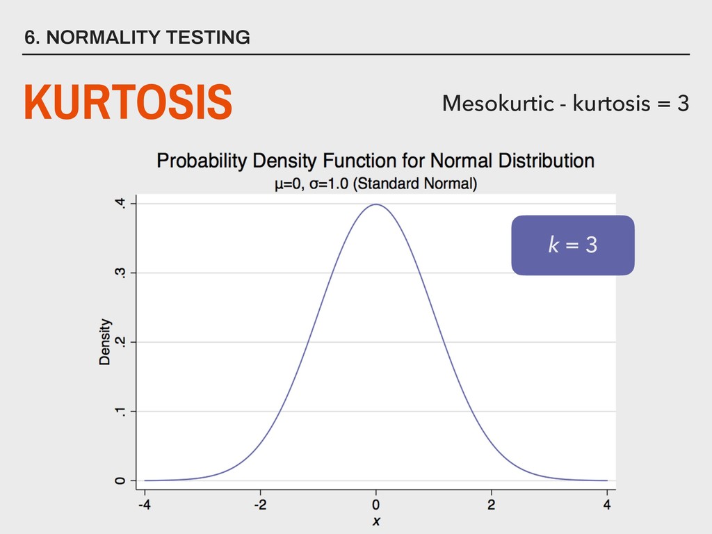
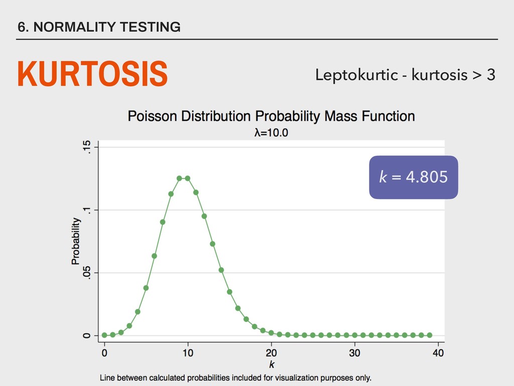
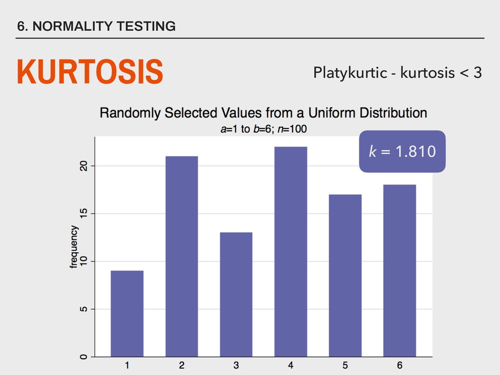
the “weight” of the tails - how many observations fall in the tails relative to the center ▸ Normal distributions have k = 3 where k is always positive and k ≥ 1. ▸ Normal distributions have k = 0 excess kurtosis (ek = k-3) where ek can be negative. ▸ k > 5 is one rule of thumb for problematic distributions 6. NORMALITY TESTING KURTOSIS
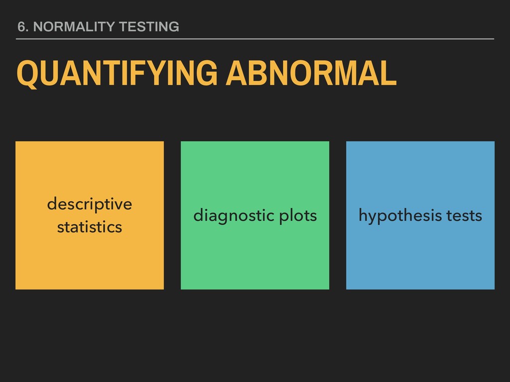
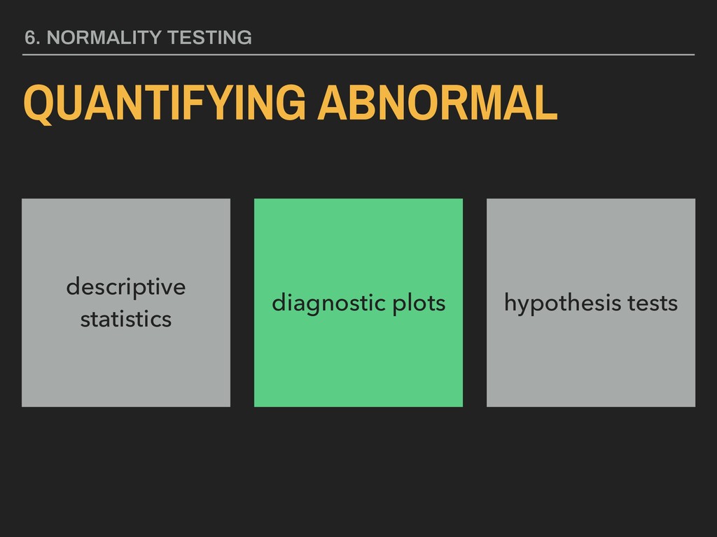
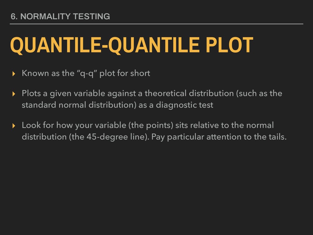
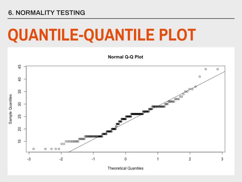
▸ Plots a given variable against a theoretical distribution (such as the standard normal distribution) as a diagnostic test ▸ Look for how your variable (the points) sits relative to the normal distribution (the 45-degree line). Pay particular attention to the tails. 6. NORMALITY TESTING
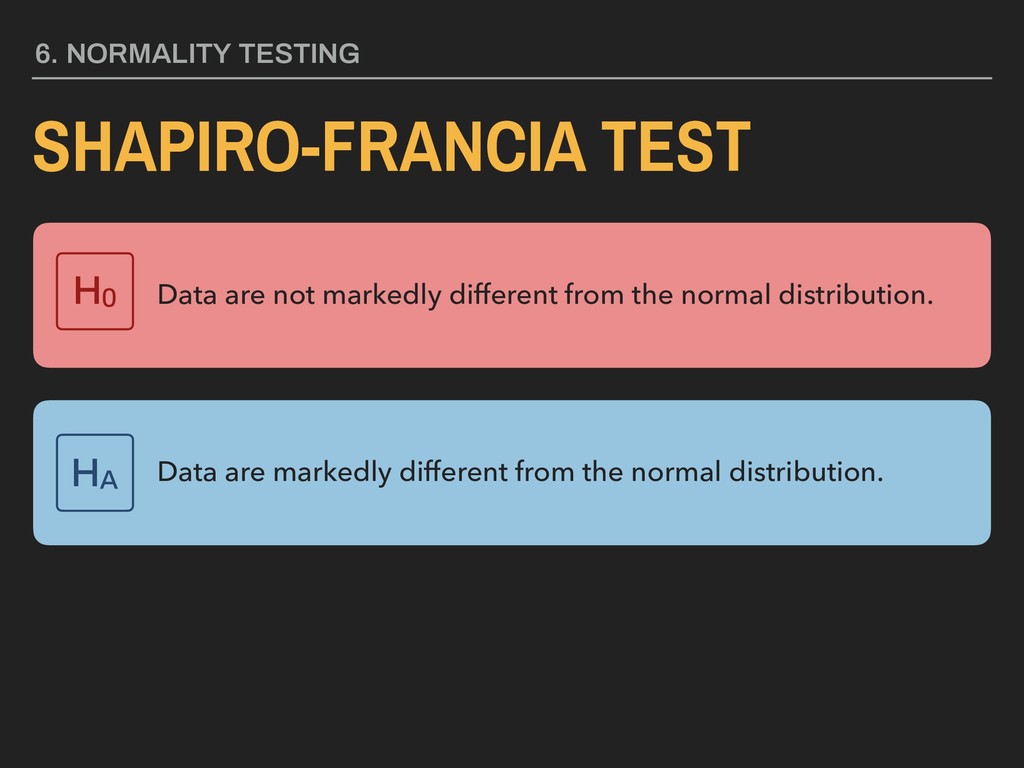
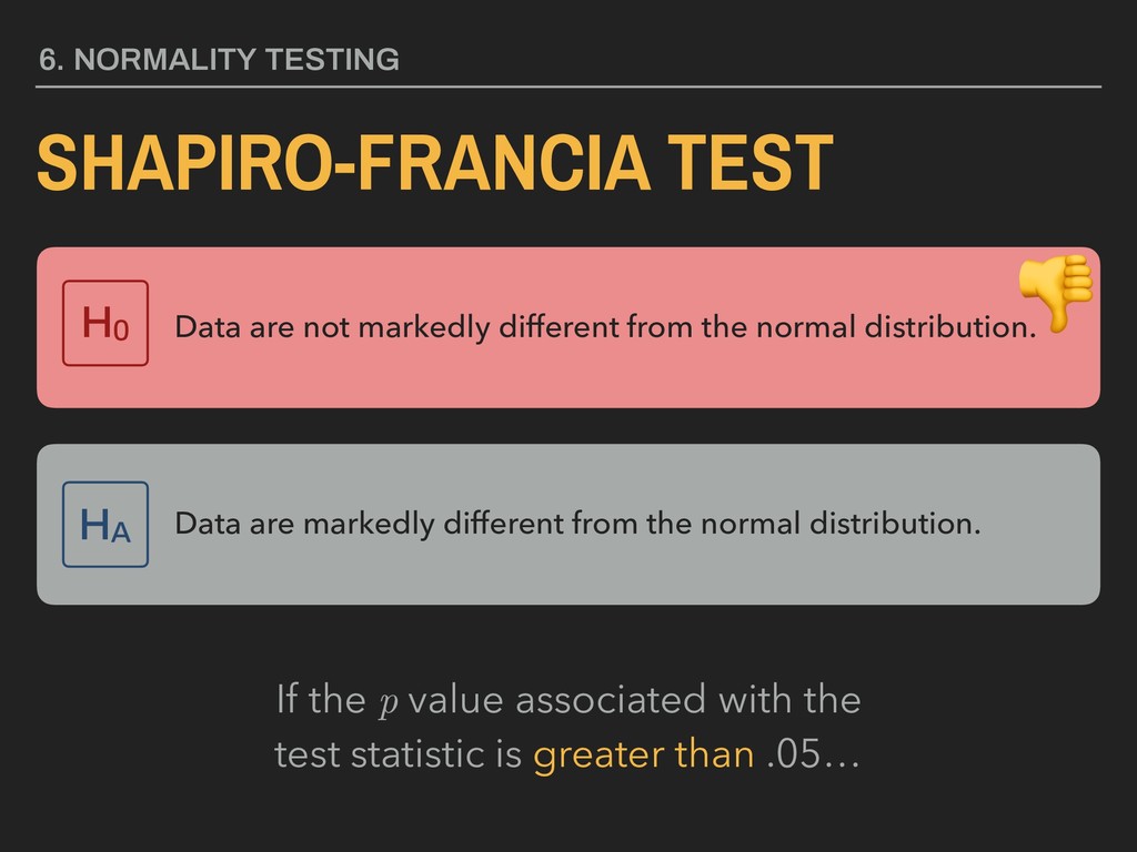
from the normal distribution. H0 Data are markedly different from the normal distribution. HA If the p value associated with the test statistic is greater than .05…
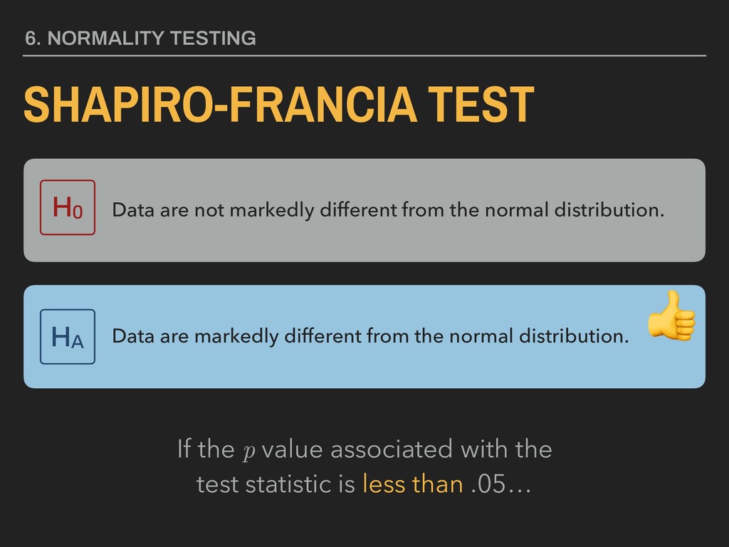
from the normal distribution. H0 Data are markedly different from the normal distribution. HA If the p value associated with the test statistic is less than .05…
06 are due before the next lecture. There was an update on the final project due today as an issue in your final project GitHub repo (DoeProject if your last name is “Doe”)