SOC 4650 & SOC 5650 - Lecture 09

Slides for Lecture 09 of the Saint Louis University Course Introduction to GIS. These slides introduce table joins in R and spatial joins in ArcMap.

Transcript

1. SPATIAL JOINS INTRO TO GISC CHRISTOPHER PRENER, PH.D. SPRING, 2018 WEEK 10 LECTURE 09
2. AGENDA INTRO TO GISC / WEEK 10 / LECTURE 09 1. Front Matter 2. GISc & Public Policy 3. Table Joins in R 4. Spatial Joins in ArcMap 5. Back Matter
3. 1 FRONT 
 MATTER
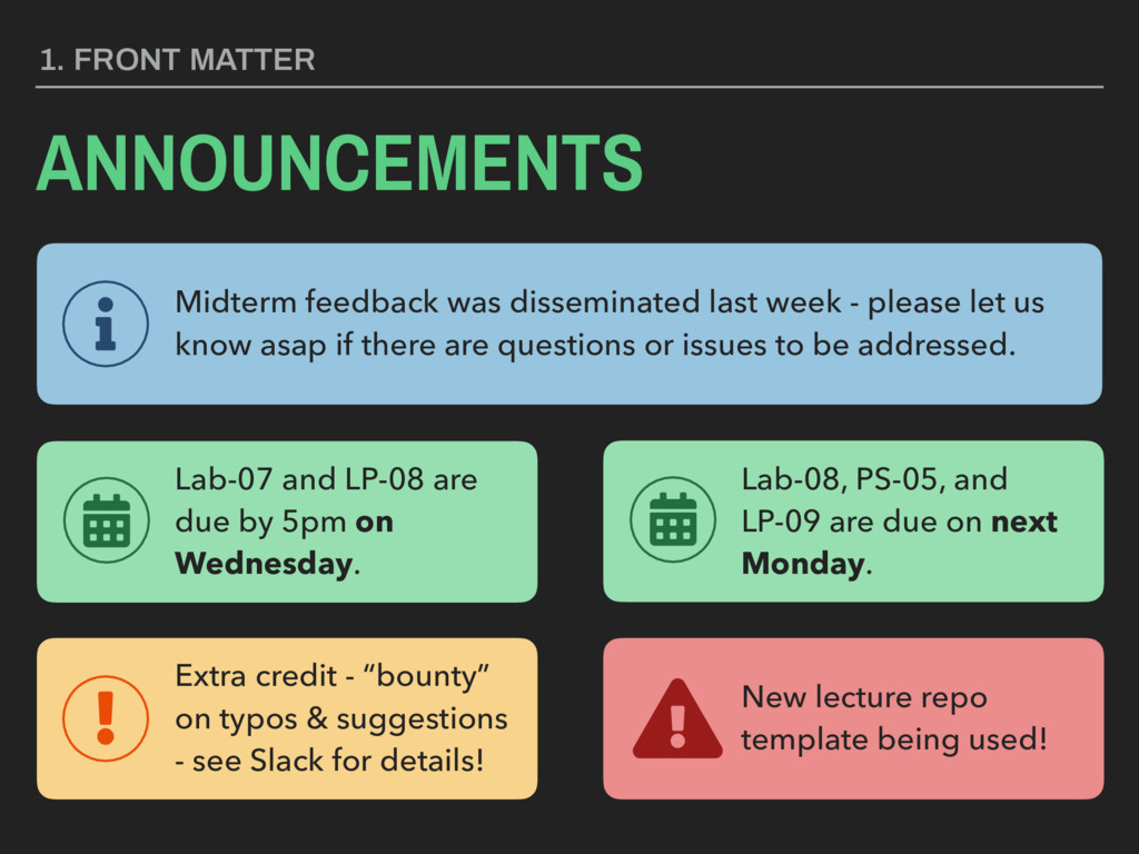
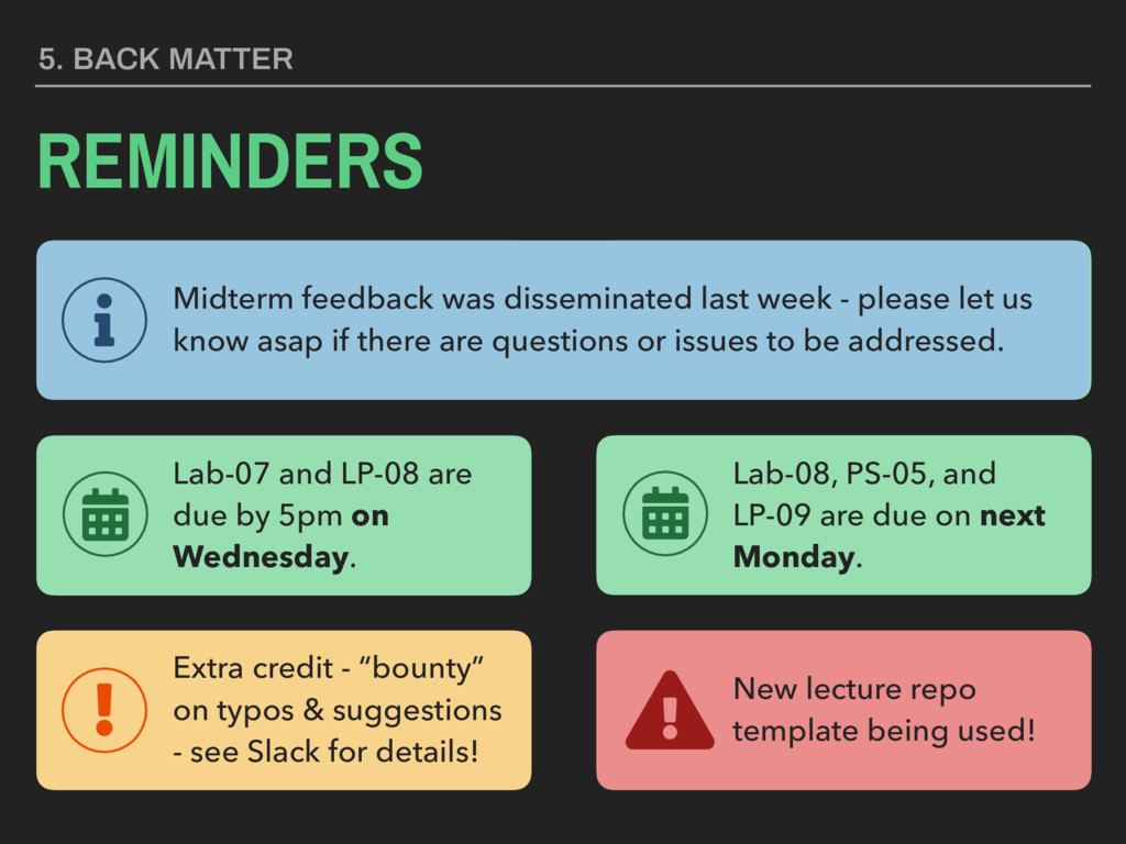
4. 1. FRONT MATTER ANNOUNCEMENTS Midterm feedback was disseminated last week - please let us know asap if there are questions or issues to be addressed. New lecture repo template being used! Extra credit - “bounty” on typos & suggestions - see Slack for details! Lab-08, PS-05, and LP-09 are due on next Monday. Lab-07 and LP-08 are due by 5pm on Wednesday.
5. GISC & PUBLIC POLICY 2
6. TABLE JOINS IN R 3
7. KEY TERM Table joins are a set of 
 techniques for combing
 the variables of two sets of 
 tabular data into a single data set. They are completed based on shared attributes.
8. KEY TERM A left join combines
 the variables of the first
 specified table with the 
 variables of the second specified 
 table based on a common ID variable.
9. 3. TABLE JOINS IN R CONCEPTUALIZING JOINS id a
10. 3. TABLE JOINS IN R CONCEPTUALIZING JOINS id a id b +
11. 3. TABLE JOINS IN R CONCEPTUALIZING JOINS id a 1 2 3 4 5 id b 1 2 3 4 5 == ✔
12. 3. TABLE JOINS IN R CONCEPTUALIZING JOINS id a 1 2 3 4 5 id b a b c d e != ✘
13. 3. TABLE JOINS IN R CONCEPTUALIZING JOINS id a 1 2 3 4 5 id b 1 2 3 4 4 != ✘
14. 3. TABLE JOINS IN R CONCEPTUALIZING JOINS id a 1 2 3 4 5 id b 1 2 3 4 4 != x y
15. 3. TABLE JOINS IN R CONCEPTUALIZING JOINS id a 1 2 3 4 5 id b 1 2 3 4 4 != x y x <- mutate(x, id =
 as.character(id))
16. 3. TABLE JOINS IN R CONCEPTUALIZING JOINS id a 1 2 3 4 5 id b 1 2 3 4 4 == x <- mutate(x, id =
 as.character(id)) ✔
17. 3. TABLE JOINS IN R CONCEPTUALIZING JOINS id a 1 2 3 4 5 id b 1 2 3 4 4 != x y y <- mutate(y, id = 
 as.numeric(id))
18. 3. TABLE JOINS IN R CONCEPTUALIZING JOINS id a 1 2 3 4 5 id b 1 2 3 4 4 == y <- mutate(y, id =
 as.character(id)) ✔
19. 3. TABLE JOINS IN R CONCEPTUALIZING JOINS id a 1 2 3 4 5 id b 1 2 3 4 5 id a b 1 2 3 4 5 + =
20. 3. TABLE JOINS IN R CONCEPTUALIZING JOINS id a 1 2 3 4 5 id a 1 2 3 4 5 id a.x a.y 1 2 3 4 5 + =
21. 3. TABLE JOINS IN R CONCEPTUALIZING JOINS id a 1 2 3 4 5 id geo 1 2 3 4 5 id a geo 1 2 3 4 5 + =
22. 3. TABLE JOINS IN R CONCEPTUALIZING JOINS id a geo 1 2 3 4 5
23. 3. TABLE JOINS IN R CONCEPTUALIZING JOINS Use to combine tabular data with geometric
 data to create choropleth maps. id a geo 1 2 3 4 5 ➜ 1 4 5 3 2
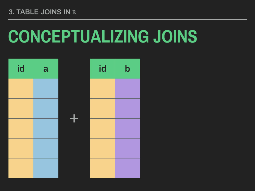
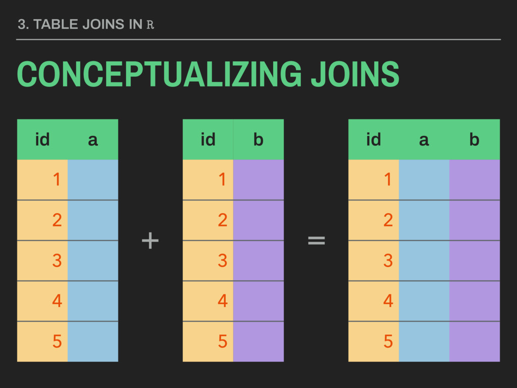
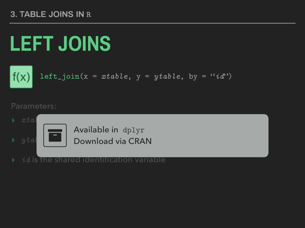
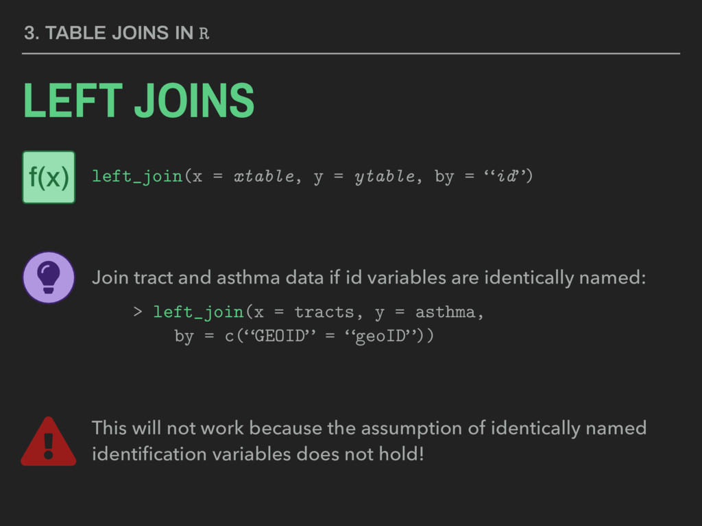
24. ▸ xtable is the table whose columns will appear first ▸ ytable is the table whose columns will appear second ▸ id is the shared identification variable Available in dplyr
 Download via CRAN 3. TABLE JOINS IN R LEFT JOINS Parameters: left_join(x = xtable, y = ytable, by = “id”) f(x)
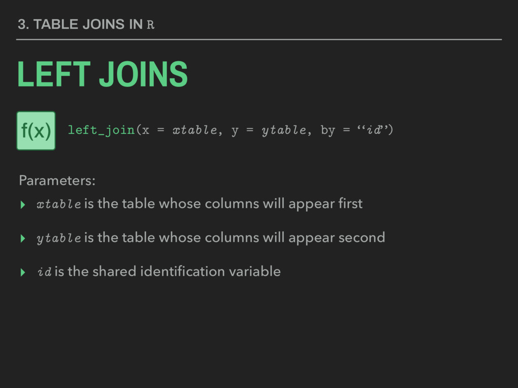
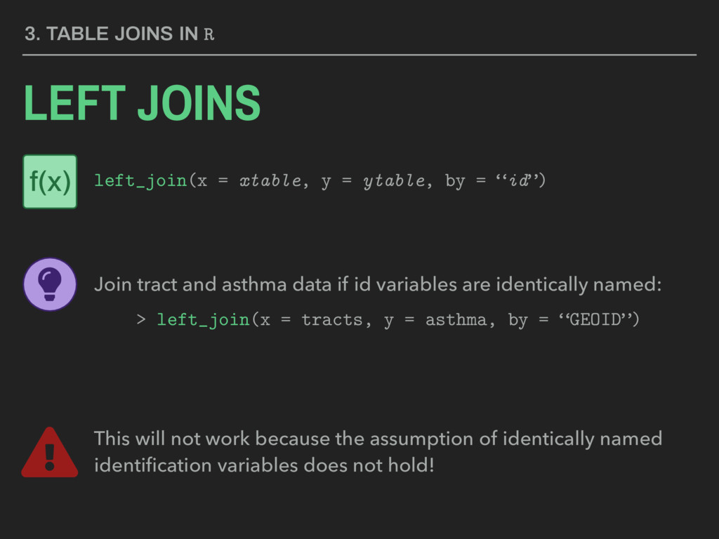
25. ▸ xtable is the table whose columns will appear first ▸ ytable is the table whose columns will appear second ▸ id is the shared identification variable 3. TABLE JOINS IN R LEFT JOINS Parameters: left_join(x = xtable, y = ytable, by = “id”) f(x)
26. LEFT JOINS > # example set-up > > library(stlData) > > tracts <- stl_sf_tracts > asthma <- stl_tbl_asthma 3. TABLE JOINS IN R
27. LEFT JOINS > tracts Simple feature collection with 106 features and 12 fields geometry type: POLYGON dimension: XY bbox: xmin: -90.32052 ymin: 38.53185 xmax: -90.16657 ymax: 38.77443 epsg (SRID): 4269 proj4string: +proj=longlat +ellps=GRS80 +towgs84=0,0,0,0,0,0,0 +no_defs First 10 features: STATEFP COUNTYFP TRACTCE GEOID NAME NAMELSAD MTFCC FUNCSTAT ALAND AWATER 313 29 510 112100 29510112100 1121 Census Tract 1121 G5020 S 6936664 0 314 29 510 116500 29510116500 1165 Census Tract 1165 G5020 S 904024 0 324 29 510 110300 29510110300 1103 Census Tract 1103 G5020 S 938287 0 536 29 510 103700 29510103700 1037 Census Tract 1037 G5020 S 910953 0 537 29 510 103800 29510103800 1038 Census Tract 1038 G5020 S 1640334 35369 538 29 510 104500 29510104500 1045 Census Tract 1045 G5020 S 1939712 0 539 29 510 106100 29510106100 1061 Census Tract 1061 G5020 S 962321 0 3. TABLE JOINS IN R
28. LEFT JOINS > tracts Simple feature collection with 106 features and 12 fields geometry type: POLYGON dimension: XY bbox: xmin: -90.32052 ymin: 38.53185 xmax: -90.16657 ymax: 38.77443 epsg (SRID): 4269 proj4string: +proj=longlat +ellps=GRS80 +towgs84=0,0,0,0,0,0,0 +no_defs First 10 features: STATEFP COUNTYFP TRACTCE GEOID NAME NAMELSAD MTFCC FUNCSTAT ALAND AWATER 313 29 510 112100 29510112100 1121 Census Tract 1121 G5020 S 6936664 0 314 29 510 116500 29510116500 1165 Census Tract 1165 G5020 S 904024 0 324 29 510 110300 29510110300 1103 Census Tract 1103 G5020 S 938287 0 536 29 510 103700 29510103700 1037 Census Tract 1037 G5020 S 910953 0 537 29 510 103800 29510103800 1038 Census Tract 1038 G5020 S 1640334 35369 538 29 510 104500 29510104500 1045 Census Tract 1045 G5020 S 1939712 0 539 29 510 106100 29510106100 1061 Census Tract 1061 G5020 S 962321 0 3. TABLE JOINS IN R
29. LEFT JOINS > asthma # A tibble: 106 x 6 geoID tractCE nameLSAD pctAsthma pctAsthma_Low pctAsthma_High <chr> <int> <chr> <dbl> <dbl> <dbl> 1 29510118100 118100 Census Tract 1181 11.9 11.1 12.7 2 29510117400 117400 Census Tract 1174 9.60 9.30 10.0 3 29510126700 126700 Census Tract 1267 14.5 13.5 15.5 4 29510119102 119102 Census Tract 1191.02 9.00 8.50 9.70 5 29510126800 126800 Census Tract 1268 9.30 8.80 9.80 6 29510126900 126900 Census Tract 1269 13.6 12.6 14.6 7 29510108100 108100 Census Tract 1081 12.7 11.8 13.8 8 29510127000 127000 Census Tract 1270 12.8 11.7 14.2 9 29510127400 127400 Census Tract 1274 12.7 11.9 13.8 10 29510103700 103700 Census Tract 1037 8.60 8.10 9.20 # ... with 96 more rows 3. TABLE JOINS IN R
30. LEFT JOINS > asthma # A tibble: 106 x 6 geoID tractCE nameLSAD pctAsthma pctAsthma_Low pctAsthma_High <chr> <int> <chr> <dbl> <dbl> <dbl> 1 29510118100 118100 Census Tract 1181 11.9 11.1 12.7 2 29510117400 117400 Census Tract 1174 9.60 9.30 10.0 3 29510126700 126700 Census Tract 1267 14.5 13.5 15.5 4 29510119102 119102 Census Tract 1191.02 9.00 8.50 9.70 5 29510126800 126800 Census Tract 1268 9.30 8.80 9.80 6 29510126900 126900 Census Tract 1269 13.6 12.6 14.6 7 29510108100 108100 Census Tract 1081 12.7 11.8 13.8 8 29510127000 127000 Census Tract 1270 12.8 11.7 14.2 9 29510127400 127400 Census Tract 1274 12.7 11.9 13.8 10 29510103700 103700 Census Tract 1037 8.60 8.10 9.20 # ... with 96 more rows 3. TABLE JOINS IN R
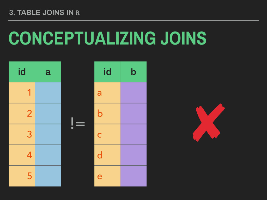
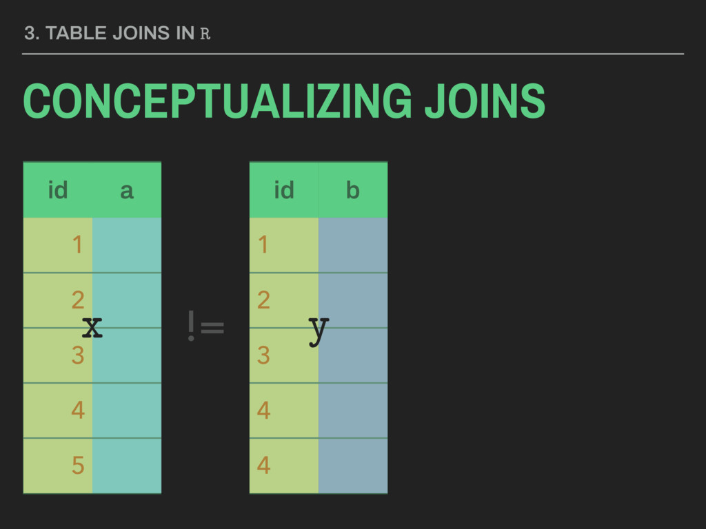
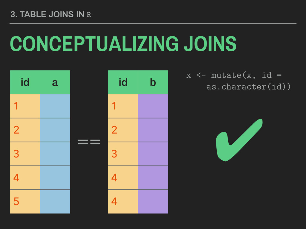
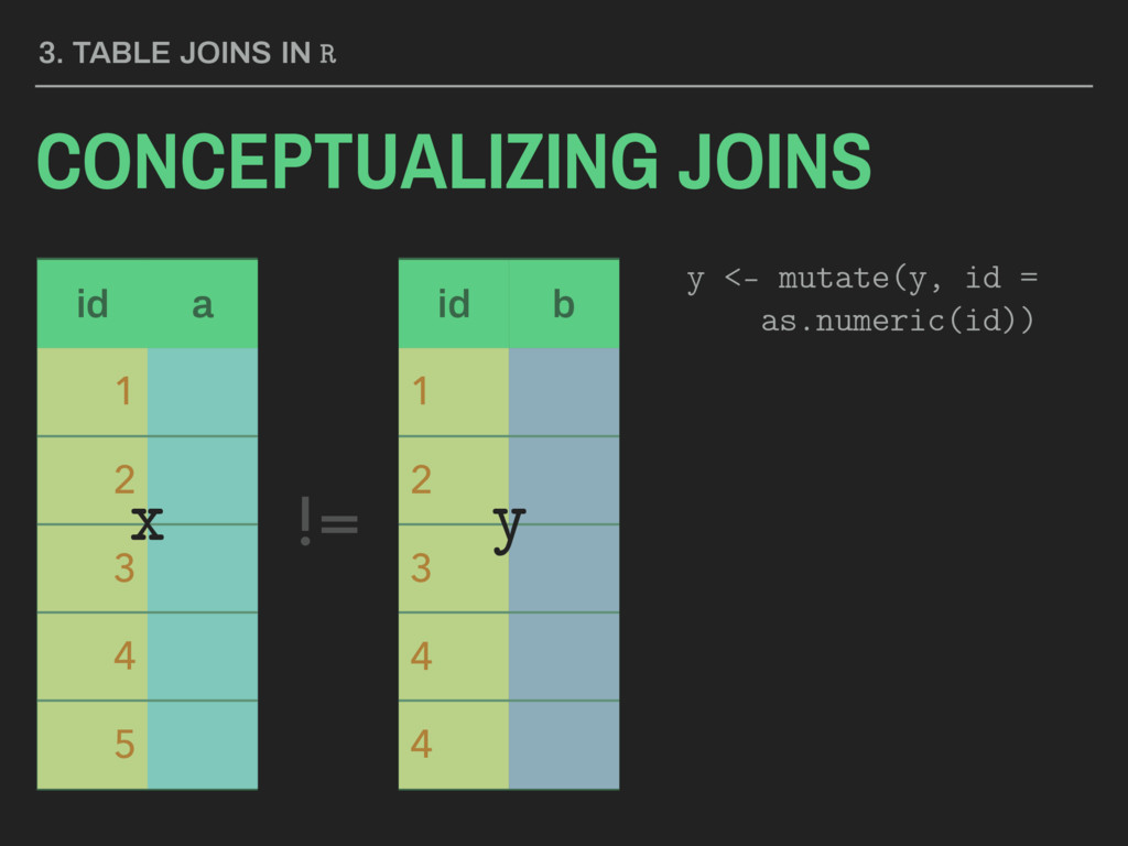
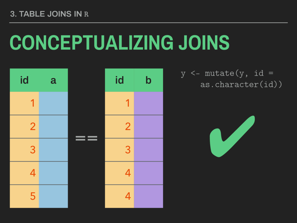
31. LEFT JOINS > class(tracts$GEOID) [1] “character” > > is.character(tracts$GEOID) [1] TRUE > > is.numeric(tracts$GEOID) [1] FALSE > > class(asthma$geoID) [1] "character" 3. TABLE JOINS IN R ▸ We can use the base R functions class(), is.character(), and is.numeric() to identify if the two identification variables are the same type. ▸ We can also do this visually, by inspecting objects in the global environment tab or using dplyr’s glimpse() function.
32. LEFT JOINS > class(tracts$GEOID) [1] “character” > > is.character(tracts$GEOID) [1] TRUE > > is.numeric(tracts$GEOID) [1] FALSE > > class(asthma$geoID) [1] "character" 3. TABLE JOINS IN R ▸ Finally, we want to note if our identification variables are identically named. ▸ If they are, we can proceed with the join. ▸ If they are not, we need to modify the join syntax or rename one of the variables.
33. LEFT JOINS 3. TABLE JOINS IN R left_join(x = xtable, y = ytable, by = “id”) Join tract and asthma data if id variables are identically named: > left_join(x = tracts, y = asthma, by = “GEOID”) This will not work because the assumption of identically named identification variables does not hold! f(x)
34. LEFT JOINS 3. TABLE JOINS IN R left_join(x = xtable, y = ytable, by = “id”) Join tract and asthma data if id variables are identically named: > left_join(x = tracts, y = asthma, 
 by = c(“GEOID” = “geoID”)) This will not work because the assumption of identically named identification variables does not hold! f(x)
35. SPATIAL JOINS IN ARCMAP 4
36. KEY TERM Spatial joins are a set of 
 techniques for combining
 or summarizing the variables
 from two geometric data sets into a single data set. They are completed based on spatial proximity.
37. KEY TERM A point to polygon join
 can provide a count or
 mean of point values that 
 that is proximate to it.
38. 5. SPATIAL JOINS IN ARCMAP CONCEPTUALIZING POINT TO POLYGON ID Shape 22 Polygon 23 Polygon 24 Polygon Target Layer 23 22 24
39. 5. SPATIAL JOINS IN ARCMAP CONCEPTUALIZING POINT TO POLYGON Target Layer 23 22 24 ID Shape Count 22 Polygon 6 23 Polygon 11 24 Polygon 5
40. KEY TERM A polygon to point join
 will append the attributes
 of a polygon to each point
 that is proximate to it.
41. CONCEPTUALIZING POLYGON TO POINT ID Shape 22 Polygon 23 Polygon 24 Polygon Reference Layer 23 22 24 ID Shape 102 Point 103 Point 104 Point 105 Point 106 Point 107 Point 108 Point 109 Point Target Layer
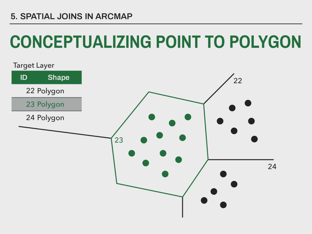
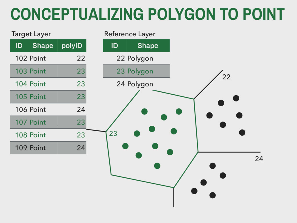
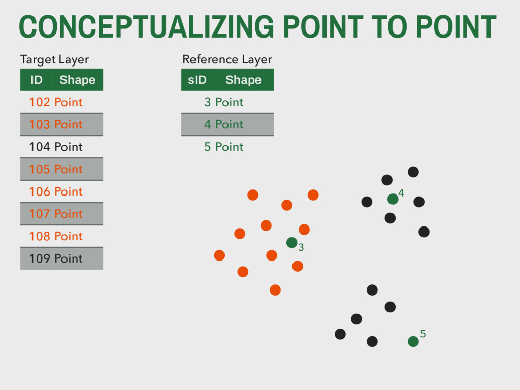
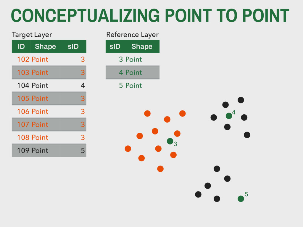
42. CONCEPTUALIZING POLYGON TO POINT ID Shape 22 Polygon 23 Polygon 24 Polygon Reference Layer 23 22 24 ID Shape polyID 102 Point 22 103 Point 23 104 Point 23 105 Point 23 106 Point 24 107 Point 23 108 Point 23 109 Point 24 Target Layer
43. KEY TERM A point to point join
 will append the attributes
 of a point to each point
 that is proximate to it.
44. CONCEPTUALIZING POINT TO POINT Reference Layer Target Layer ID Shape 102 Point 103 Point 104 Point 105 Point 106 Point 107 Point 108 Point 109 Point sID Shape 3 Point 4 Point 5 Point 3 4 5
45. CONCEPTUALIZING POINT TO POINT Reference Layer Target Layer ID Shape sID 102 Point 3 103 Point 3 104 Point 4 105 Point 3 106 Point 3 107 Point 3 108 Point 3 109 Point 5 sID Shape 3 Point 4 Point 5 Point 3 4 5
46. 5 BACK 
 MATTER
47. AGENDA REVIEW 5. BACK MATTER 2. GISc & Public Policy 3. Table Joins in R 4. Spatial Joins in ArcMap
48. Caution Text REMINDERS 5. BACK MATTER Announcement Text 5. Announcement Text Due Date Text Due Date Text Warning Text Midterm feedback was disseminated last week - please let us know asap if there are questions or issues to be addressed. New lecture repo template being used! Extra credit - “bounty” on typos & suggestions - see Slack for details! Lab-08, PS-05, and LP-09 are due on next Monday. Lab-07 and LP-08 are due by 5pm on Wednesday.