The Continuum Hypothesis, the Axiom of Choice, and Lebesgue Measurability

Transcript

1. The Continuum Hypothesis, the Axiom of Choice, and Lebesgue Measurability Chris Lambie-Hanson CMU Graduate Student Seminar 11 October 2011
2. Definitions If S is a set, then a linear order on S is a binary relation ≤ such that
3. Definitions If S is a set, then a linear order on S is a binary relation ≤ such that 1 For all x ∈ S, x ≤ x.
4. Definitions If S is a set, then a linear order on S is a binary relation ≤ such that 1 For all x ∈ S, x ≤ x. 2 For all x, y ∈ S, if x ≤ y and y ≤ x, then x = y.
5. Definitions If S is a set, then a linear order on S is a binary relation ≤ such that 1 For all x ∈ S, x ≤ x. 2 For all x, y ∈ S, if x ≤ y and y ≤ x, then x = y. 3 For all x, y, z ∈ S, if x ≤ y and y ≤ z, then x ≤ z.
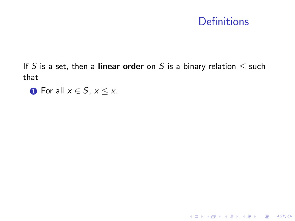
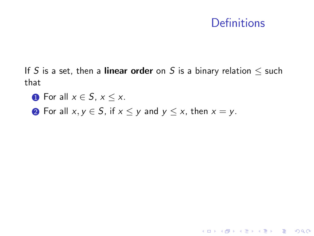
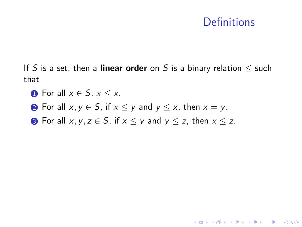
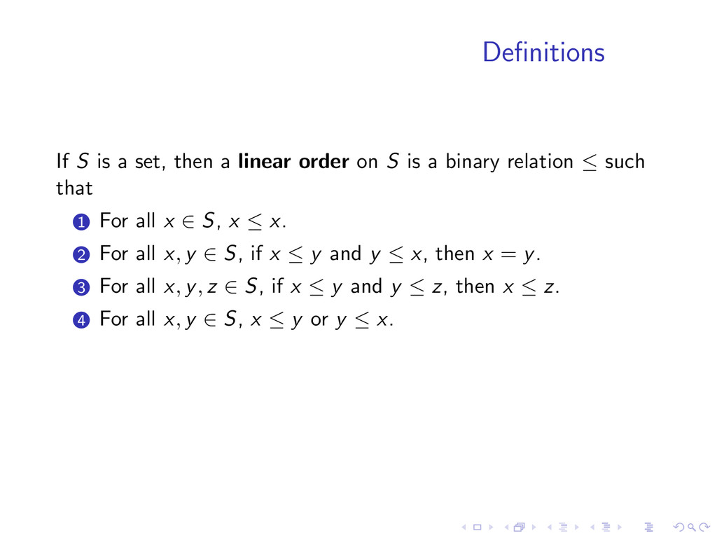
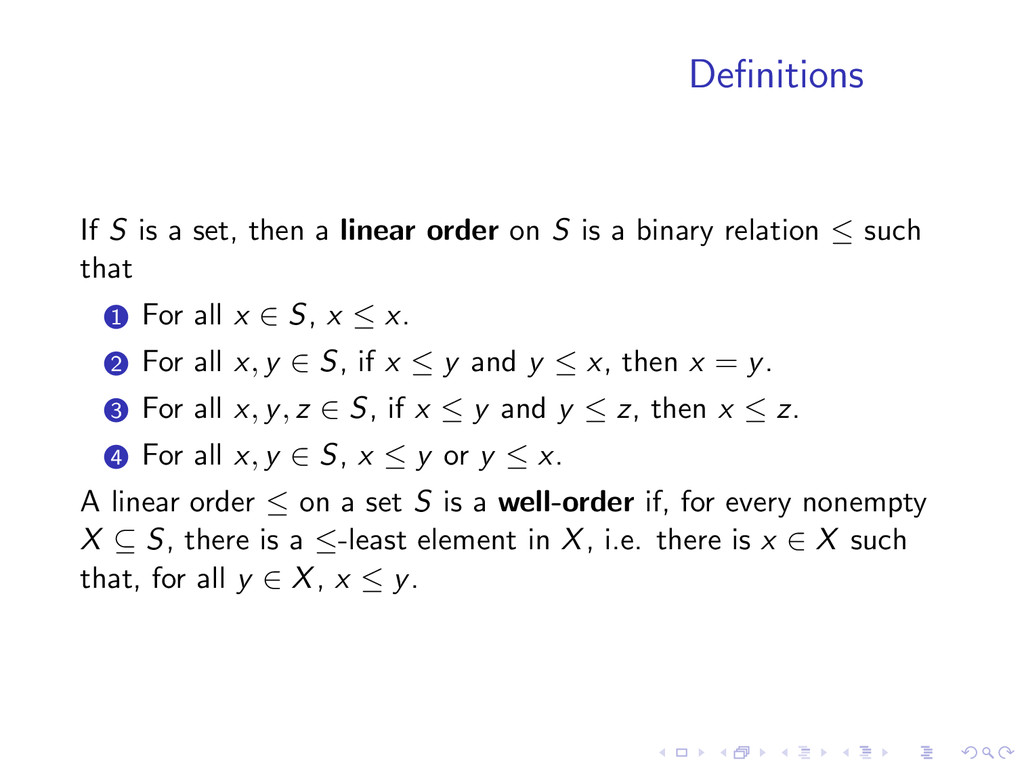
6. Definitions If S is a set, then a linear order on S is a binary relation ≤ such that 1 For all x ∈ S, x ≤ x. 2 For all x, y ∈ S, if x ≤ y and y ≤ x, then x = y. 3 For all x, y, z ∈ S, if x ≤ y and y ≤ z, then x ≤ z. 4 For all x, y ∈ S, x ≤ y or y ≤ x.
7. Definitions If S is a set, then a linear order on S is a binary relation ≤ such that 1 For all x ∈ S, x ≤ x. 2 For all x, y ∈ S, if x ≤ y and y ≤ x, then x = y. 3 For all x, y, z ∈ S, if x ≤ y and y ≤ z, then x ≤ z. 4 For all x, y ∈ S, x ≤ y or y ≤ x. A linear order ≤ on a set S is a well-order if, for every nonempty X ⊆ S, there is a ≤-least element in X, i.e. there is x ∈ X such that, for all y ∈ X, x ≤ y.
8. The Axiom of Choice The Axiom of Choice is the assertion: For every family of nonempty sets F, there is a function g such that dom(g) = F and, for every X ∈ F, g(X) ∈ X.
9. The Axiom of Choice The Axiom of Choice is the assertion: For every family of nonempty sets F, there is a function g such that dom(g) = F and, for every X ∈ F, g(X) ∈ X. The Axiom of Choice is equivalent to the Well-ordering Theorem, which asserts that every set can be well-ordered.
10. Ordinals, Informally An ordinal number describes the order type of a well-ordering.
11. Ordinals, Informally An ordinal number describes the order type of a well-ordering. • A natural number n is an ordinal describing a well-ordering with n elements.
12. Ordinals, Informally An ordinal number describes the order type of a well-ordering. • A natural number n is an ordinal describing a well-ordering with n elements. • The ordinal describing the order type of the natural numbers is ω.
13. Ordinals, Informally An ordinal number describes the order type of a well-ordering. • A natural number n is an ordinal describing a well-ordering with n elements. • The ordinal describing the order type of the natural numbers is ω. • The ordinal describing the order type of the natural numbers plus one element larger than all of the natural numbers is ω + 1.
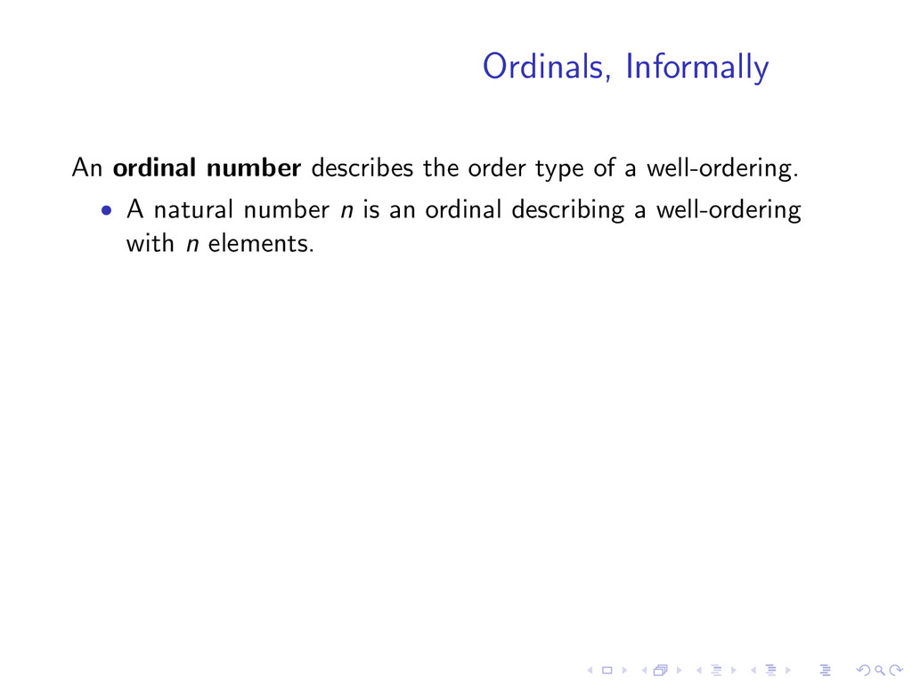
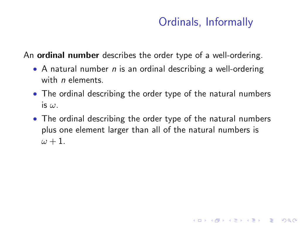
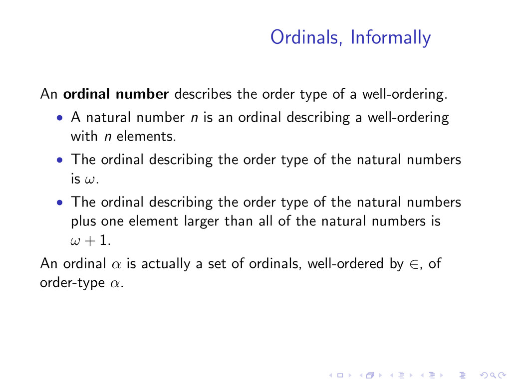
14. Ordinals, Informally An ordinal number describes the order type of a well-ordering. • A natural number n is an ordinal describing a well-ordering with n elements. • The ordinal describing the order type of the natural numbers is ω. • The ordinal describing the order type of the natural numbers plus one element larger than all of the natural numbers is ω + 1. An ordinal α is actually a set of ordinals, well-ordered by ∈, of order-type α.
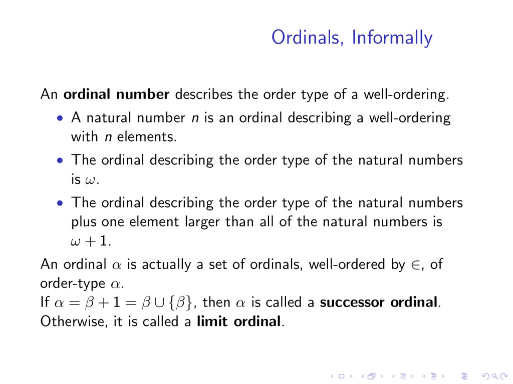
15. Ordinals, Informally An ordinal number describes the order type of a well-ordering. • A natural number n is an ordinal describing a well-ordering with n elements. • The ordinal describing the order type of the natural numbers is ω. • The ordinal describing the order type of the natural numbers plus one element larger than all of the natural numbers is ω + 1. An ordinal α is actually a set of ordinals, well-ordered by ∈, of order-type α. If α = β + 1 = β ∪ {β}, then α is called a successor ordinal. Otherwise, it is called a limit ordinal.
16. Cardinals Two sets A and B have the same cardinality if there is a bijection f : A → B.
17. Cardinals Two sets A and B have the same cardinality if there is a bijection f : A → B. The cardinality of A, written |A|, can be thought of as the equivalence class of all sets for which bijections with A exist.
18. Cardinals Two sets A and B have the same cardinality if there is a bijection f : A → B. The cardinality of A, written |A|, can be thought of as the equivalence class of all sets for which bijections with A exist. For two sets A and B, we say |A| |B| if there is an injective function f : A → B.
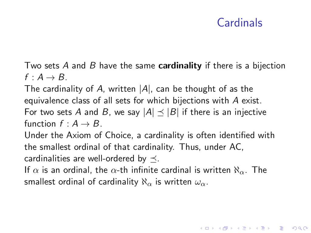
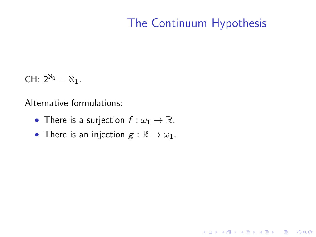
19. Cardinals Two sets A and B have the same cardinality if there is a bijection f : A → B. The cardinality of A, written |A|, can be thought of as the equivalence class of all sets for which bijections with A exist. For two sets A and B, we say |A| |B| if there is an injective function f : A → B. Under the Axiom of Choice, a cardinality is often identified with the smallest ordinal of that cardinality. Thus, under AC, cardinalities are well-ordered by .
20. Cardinals Two sets A and B have the same cardinality if there is a bijection f : A → B. The cardinality of A, written |A|, can be thought of as the equivalence class of all sets for which bijections with A exist. For two sets A and B, we say |A| |B| if there is an injective function f : A → B. Under the Axiom of Choice, a cardinality is often identified with the smallest ordinal of that cardinality. Thus, under AC, cardinalities are well-ordered by . If α is an ordinal, the α-th infinite cardinal is written ℵα. The smallest ordinal of cardinality ℵα is written ωα.
21. Cardinals A set is called countable if it is either finite or has the same cardinality as the set of natural numbers.
22. Cardinals A set is called countable if it is either finite or has the same cardinality as the set of natural numbers. Every natural number n is a cardinal number.
23. Cardinals A set is called countable if it is either finite or has the same cardinality as the set of natural numbers. Every natural number n is a cardinal number. ω0 = ω, and |ω| = ℵ0.
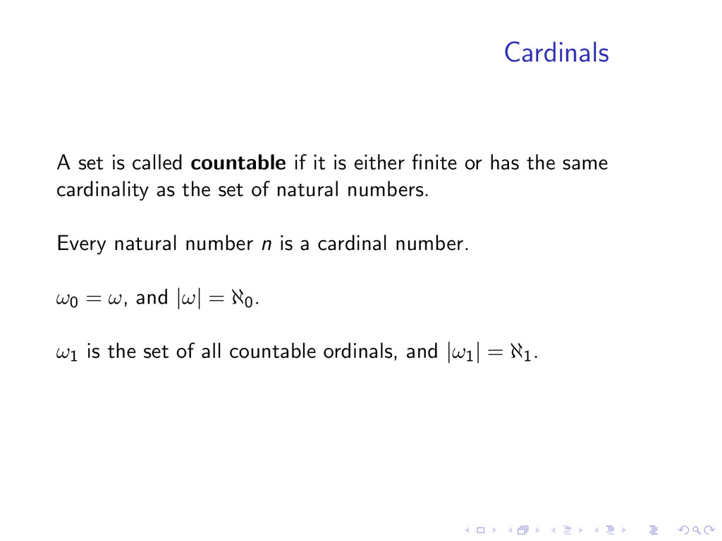
24. Cardinals A set is called countable if it is either finite or has the same cardinality as the set of natural numbers. Every natural number n is a cardinal number. ω0 = ω, and |ω| = ℵ0. ω1 is the set of all countable ordinals, and |ω1| = ℵ1.
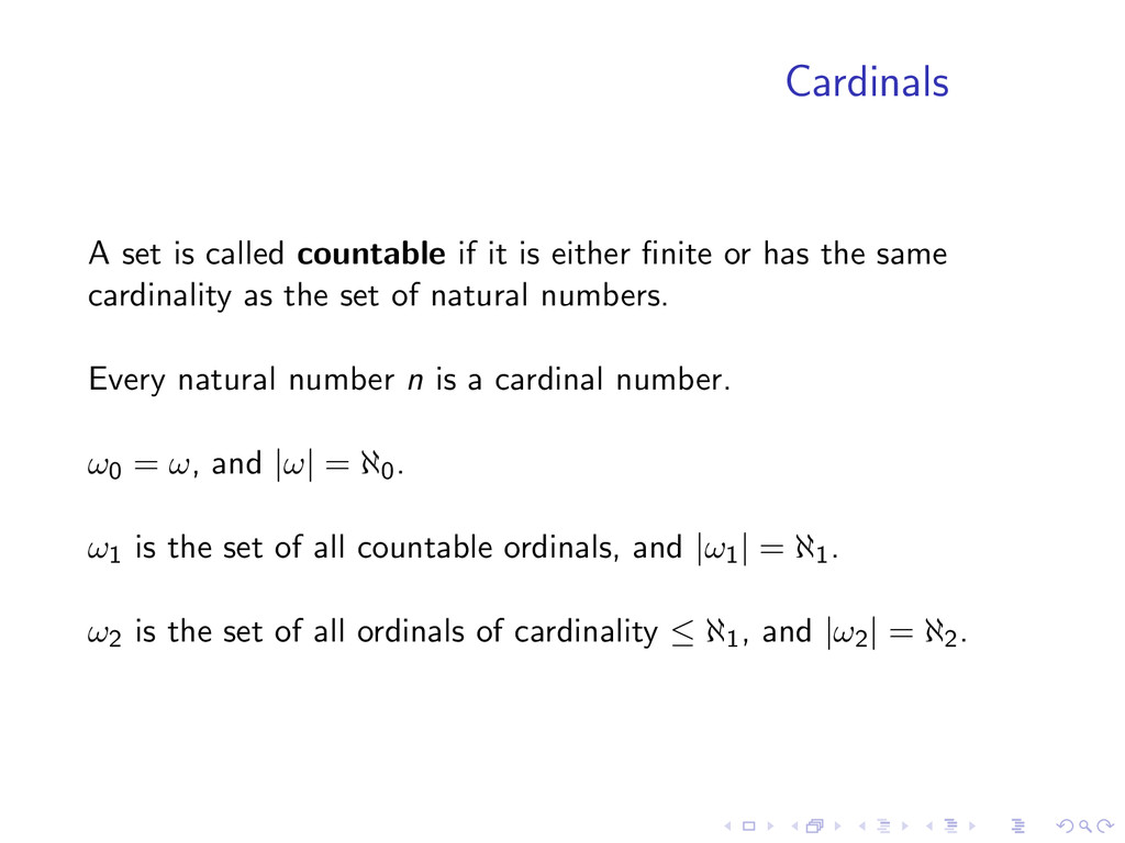
25. Cardinals A set is called countable if it is either finite or has the same cardinality as the set of natural numbers. Every natural number n is a cardinal number. ω0 = ω, and |ω| = ℵ0. ω1 is the set of all countable ordinals, and |ω1| = ℵ1. ω2 is the set of all ordinals of cardinality ≤ ℵ1, and |ω2| = ℵ2.
26. Cantor’s Theorem If A is a set, then the power set of A, written P(A), is the set of all subsets of A.
27. Cantor’s Theorem If A is a set, then the power set of A, written P(A), is the set of all subsets of A. Theorem For every set A, |A| ≺ |P(A)|.
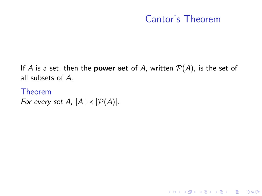
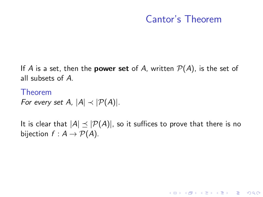
28. Cantor’s Theorem If A is a set, then the power set of A, written P(A), is the set of all subsets of A. Theorem For every set A, |A| ≺ |P(A)|. It is clear that |A| |P(A)|, so it suffices to prove that there is no bijection f : A → P(A).
29. Hypergame We say a finite game is a two-player game with alternating moves which is guaranteed to end in a finite number of moves.
30. Hypergame We say a finite game is a two-player game with alternating moves which is guaranteed to end in a finite number of moves. Hypergame is a two-player game with alternating moves played as follows:
31. Hypergame We say a finite game is a two-player game with alternating moves which is guaranteed to end in a finite number of moves. Hypergame is a two-player game with alternating moves played as follows: 1 Player 1 names a finite game.
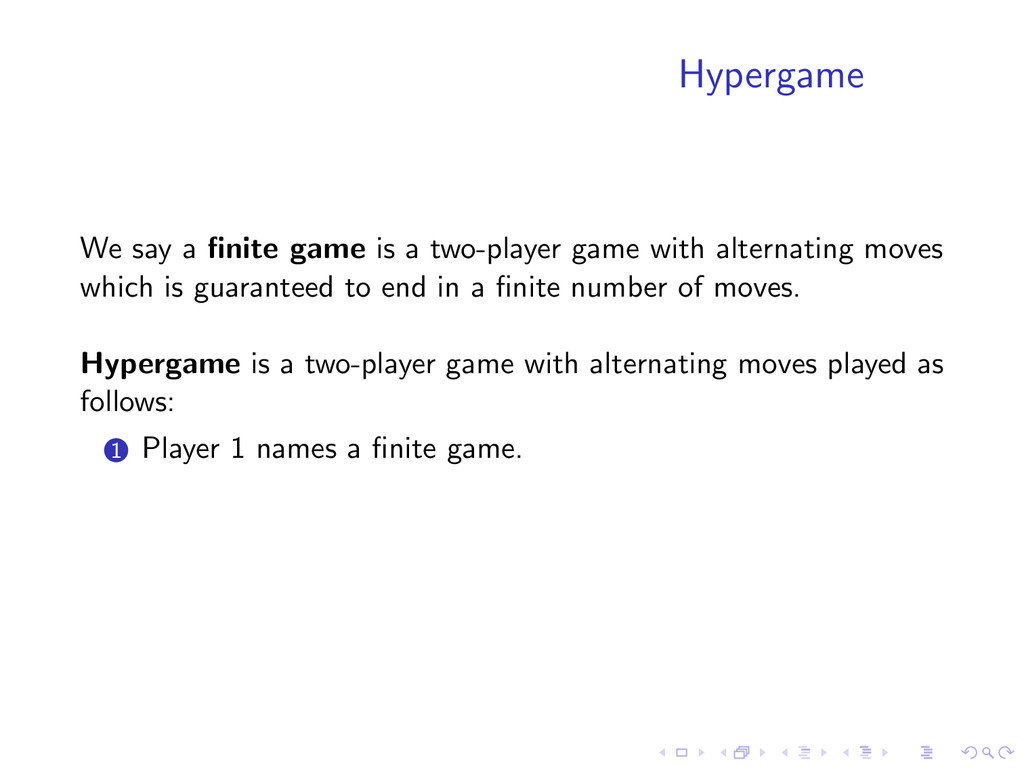
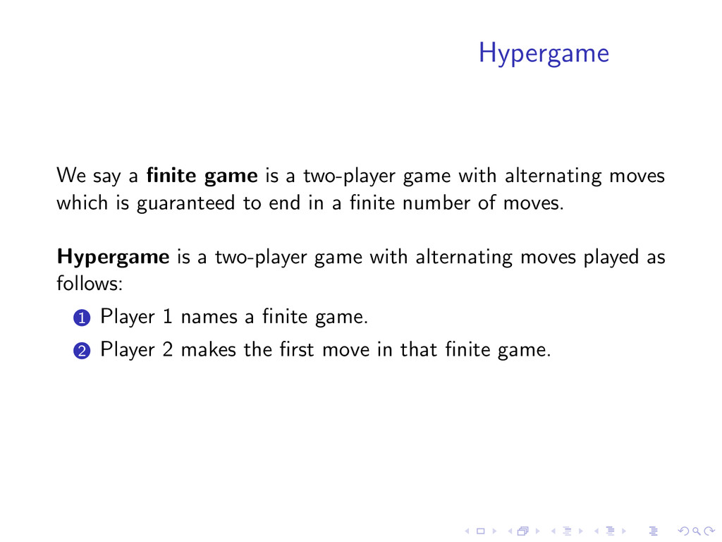
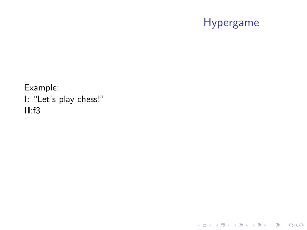
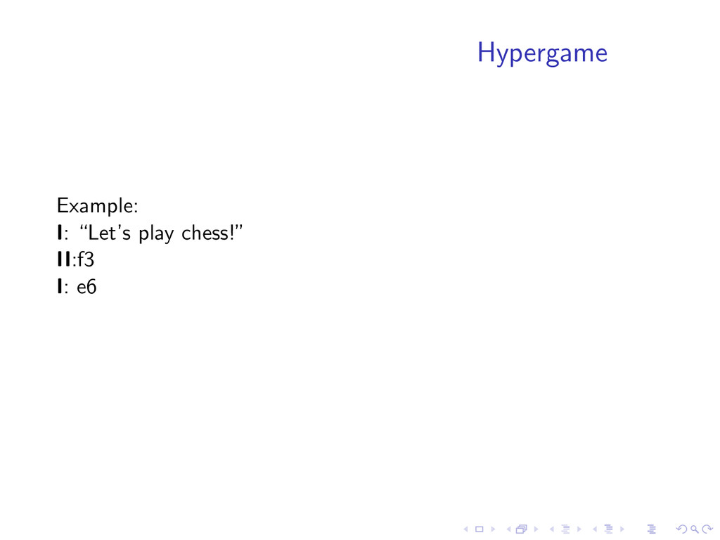
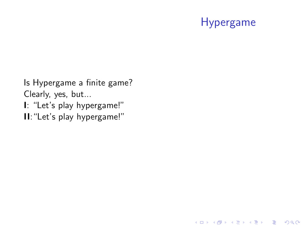
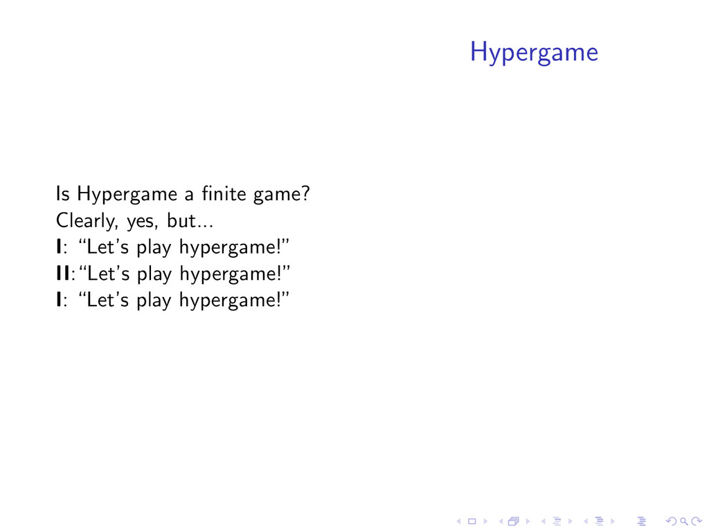
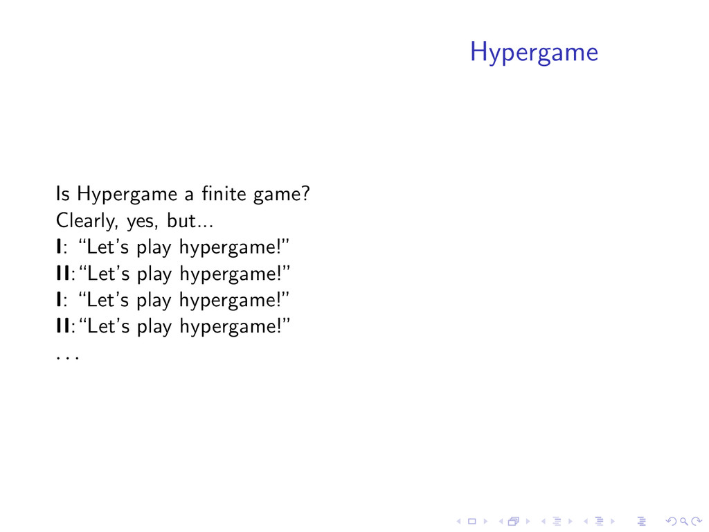
32. Hypergame We say a finite game is a two-player game with alternating moves which is guaranteed to end in a finite number of moves. Hypergame is a two-player game with alternating moves played as follows: 1 Player 1 names a finite game. 2 Player 2 makes the first move in that finite game.
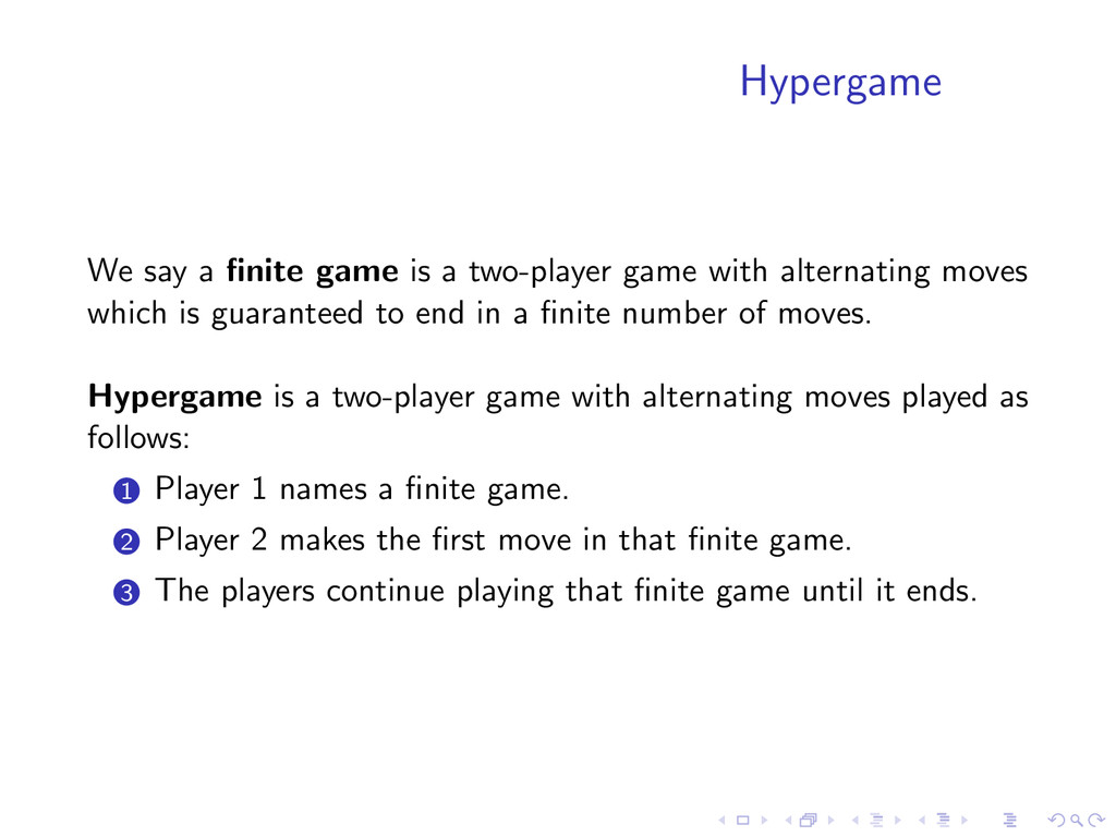
33. Hypergame We say a finite game is a two-player game with alternating moves which is guaranteed to end in a finite number of moves. Hypergame is a two-player game with alternating moves played as follows: 1 Player 1 names a finite game. 2 Player 2 makes the first move in that finite game. 3 The players continue playing that finite game until it ends.
34. Hypergame Example:
35. Hypergame Example: I: “Let’s play chess!”
36. Hypergame Example: I: “Let’s play chess!” II:f3
37. Hypergame Example: I: “Let’s play chess!” II:f3 I: e6
38. Hypergame Example: I: “Let’s play chess!” II:f3 I: e6 II:g4
39. Hypergame Example: I: “Let’s play chess!” II:f3 I: e6 II:g4 I: Qh4#
40. Hypergame Is Hypergame a finite game?
41. Hypergame Is Hypergame a finite game? Clearly, yes, but...
42. Hypergame Is Hypergame a finite game? Clearly, yes, but... I: “Let’s play hypergame!”
43. Hypergame Is Hypergame a finite game? Clearly, yes, but... I: “Let’s play hypergame!” II:“Let’s play hypergame!”
44. Hypergame Is Hypergame a finite game? Clearly, yes, but... I: “Let’s play hypergame!” II:“Let’s play hypergame!” I: “Let’s play hypergame!”
45. Hypergame Is Hypergame a finite game? Clearly, yes, but... I: “Let’s play hypergame!” II:“Let’s play hypergame!” I: “Let’s play hypergame!” II:“Let’s play hypergame!” . . .
46. Proof of Cantor’s Theorem
47. Proof of Cantor’s Theorem Suppose for sake of contradiction that there is an infinite set A and a bijection f : A → P(A).
48. Proof of Cantor’s Theorem Suppose for sake of contradiction that there is an infinite set A and a bijection f : A → P(A). We say that (a0, a1, a2, . . .) is a path in A if: 1 a0 ∈ A 2 For all n, an+1 ∈ f (an)
49. Proof of Cantor’s Theorem Suppose for sake of contradiction that there is an infinite set A and a bijection f : A → P(A). We say that (a0, a1, a2, . . .) is a path in A if: 1 a0 ∈ A 2 For all n, an+1 ∈ f (an) Let X = {a ∈ A | there is no infinite path in A starting with a}.
50. Proof of Cantor’s Theorem Suppose for sake of contradiction that there is an infinite set A and a bijection f : A → P(A). We say that (a0, a1, a2, . . .) is a path in A if: 1 a0 ∈ A 2 For all n, an+1 ∈ f (an) Let X = {a ∈ A | there is no infinite path in A starting with a}. Since f is a bijection, there is x ∈ A such that f (x) = X.
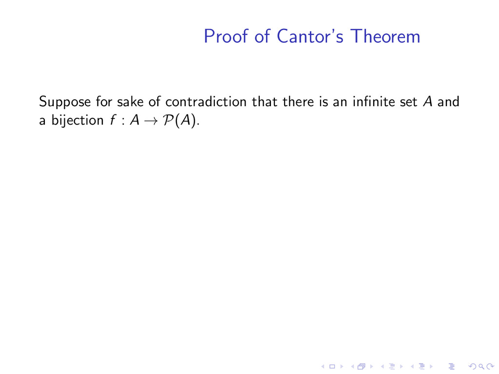
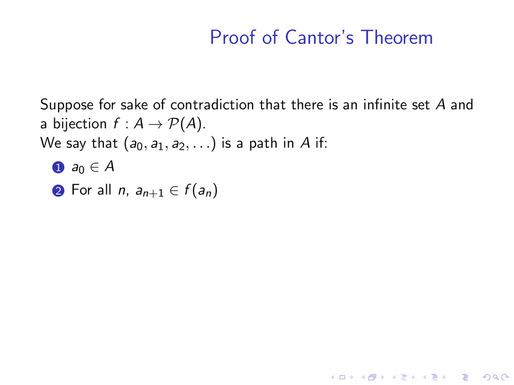
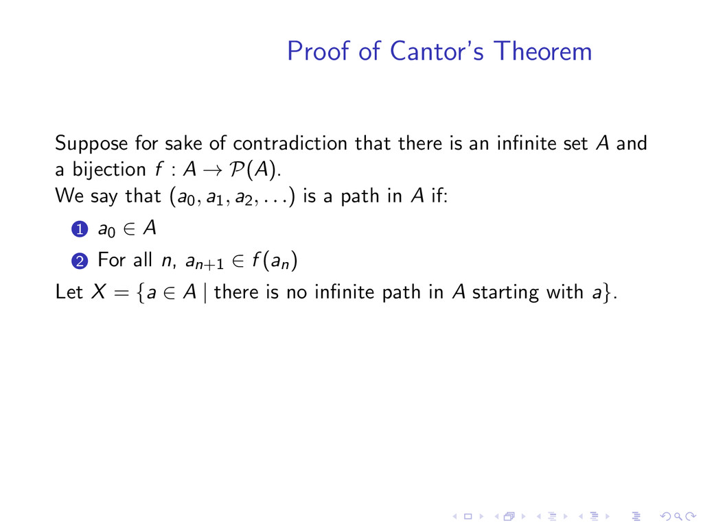
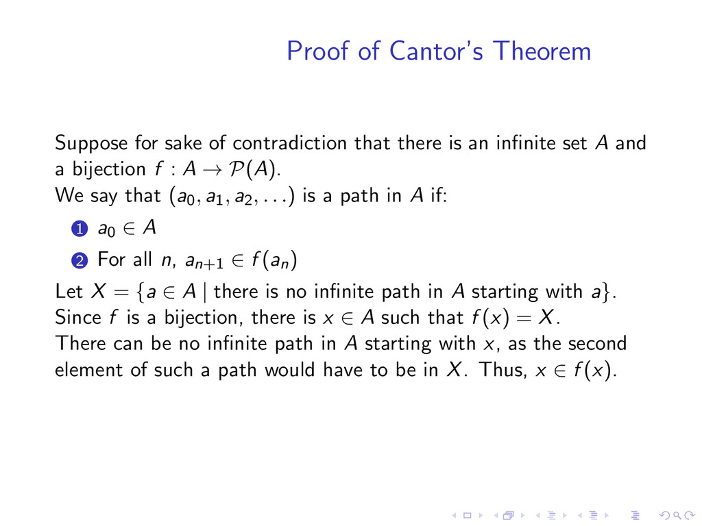
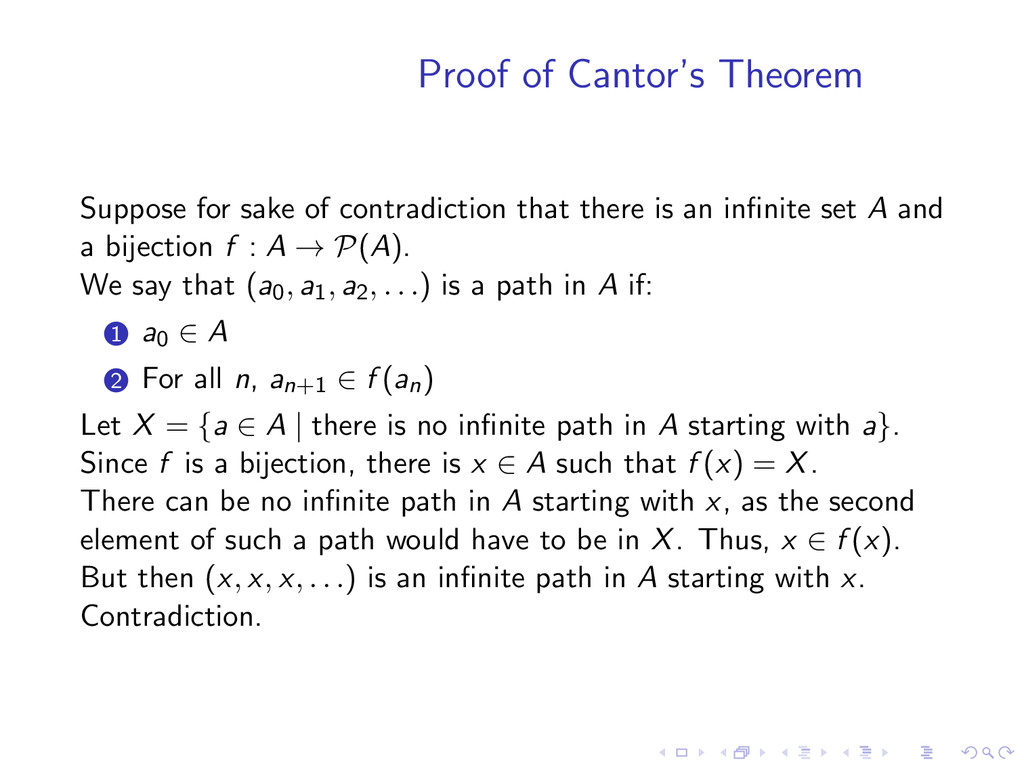
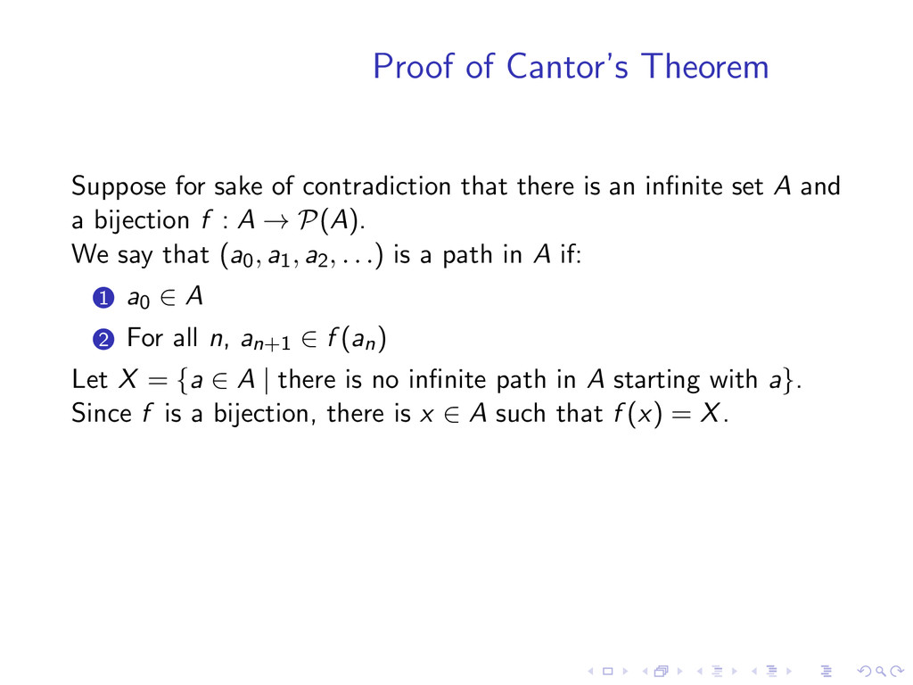
51. Proof of Cantor’s Theorem Suppose for sake of contradiction that there is an infinite set A and a bijection f : A → P(A). We say that (a0, a1, a2, . . .) is a path in A if: 1 a0 ∈ A 2 For all n, an+1 ∈ f (an) Let X = {a ∈ A | there is no infinite path in A starting with a}. Since f is a bijection, there is x ∈ A such that f (x) = X. There can be no infinite path in A starting with x, as the second element of such a path would have to be in X. Thus, x ∈ f (x).
52. Proof of Cantor’s Theorem Suppose for sake of contradiction that there is an infinite set A and a bijection f : A → P(A). We say that (a0, a1, a2, . . .) is a path in A if: 1 a0 ∈ A 2 For all n, an+1 ∈ f (an) Let X = {a ∈ A | there is no infinite path in A starting with a}. Since f is a bijection, there is x ∈ A such that f (x) = X. There can be no infinite path in A starting with x, as the second element of such a path would have to be in X. Thus, x ∈ f (x). But then (x, x, x, . . .) is an infinite path in A starting with x. Contradiction.
53. Real numbers
54. Real numbers Definition A Polish space is a separable, completely metrizable topological space.
55. Real numbers Definition A Polish space is a separable, completely metrizable topological space. Fact There is a Borel isomorphism between any two uncountable Polish spaces.
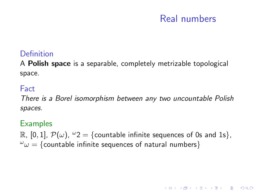
56. Real numbers Definition A Polish space is a separable, completely metrizable topological space. Fact There is a Borel isomorphism between any two uncountable Polish spaces. Examples R, [0, 1], P(ω), ω2 = {countable infinite sequences of 0s and 1s}, ωω = {countable infinite sequences of natural numbers}
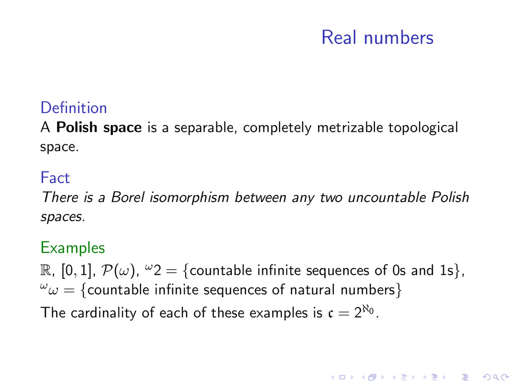
57. Real numbers Definition A Polish space is a separable, completely metrizable topological space. Fact There is a Borel isomorphism between any two uncountable Polish spaces. Examples R, [0, 1], P(ω), ω2 = {countable infinite sequences of 0s and 1s}, ωω = {countable infinite sequences of natural numbers} The cardinality of each of these examples is c = 2ℵ0 .
58. The Continuum Hypothesis CH: 2ℵ0 = ℵ1.
59. The Continuum Hypothesis CH: 2ℵ0 = ℵ1. Alternative formulations:
60. The Continuum Hypothesis CH: 2ℵ0 = ℵ1. Alternative formulations: • There is a surjection f : ω1 → R.
61. The Continuum Hypothesis CH: 2ℵ0 = ℵ1. Alternative formulations: • There is a surjection f : ω1 → R. • There is an injection g : R → ω1.
62. The Continuum Hypothesis CH: 2ℵ0 = ℵ1. Alternative formulations: • There is a surjection f : ω1 → R. • There is an injection g : R → ω1. • Every uncountable subset of R has cardinality 2ℵ0 .
63. The Continuum Hypothesis CH: 2ℵ0 = ℵ1. Alternative formulations: • There is a surjection f : ω1 → R. • There is an injection g : R → ω1. • Every uncountable subset of R has cardinality 2ℵ0 . Hilbert’s 1st problem.
64. Cantor-Bendixson Theorem
65. Cantor-Bendixson Theorem Definition If X is a topological space, then a set S ⊆ X is a perfect set if it is closed and has no isolated points.
66. Cantor-Bendixson Theorem Definition If X is a topological space, then a set S ⊆ X is a perfect set if it is closed and has no isolated points. Fact If S is a nonempty perfect subset of a Polish space, then |S| = 2ℵ0 .
67. Cantor-Bendixson Theorem Definition If X is a topological space, then a set S ⊆ X is a perfect set if it is closed and has no isolated points. Fact If S is a nonempty perfect subset of a Polish space, then |S| = 2ℵ0 . Definition A subset A of a Polish space has the perfect set property if either A is countable or A contains a nonempty perfect subset.
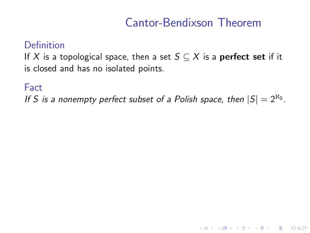
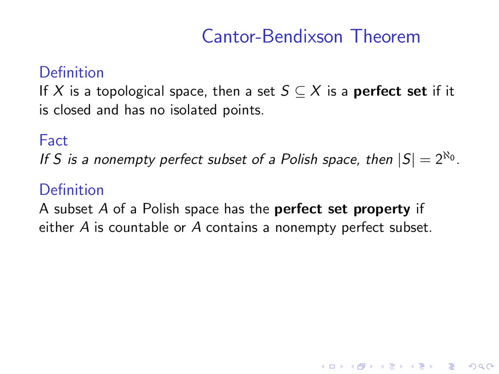
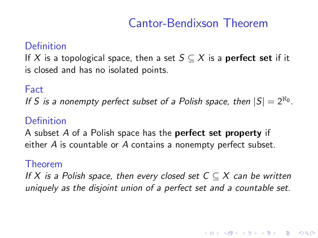
68. Cantor-Bendixson Theorem Definition If X is a topological space, then a set S ⊆ X is a perfect set if it is closed and has no isolated points. Fact If S is a nonempty perfect subset of a Polish space, then |S| = 2ℵ0 . Definition A subset A of a Polish space has the perfect set property if either A is countable or A contains a nonempty perfect subset. Theorem If X is a Polish space, then every closed set C ⊆ X can be written uniquely as the disjoint union of a perfect set and a countable set.
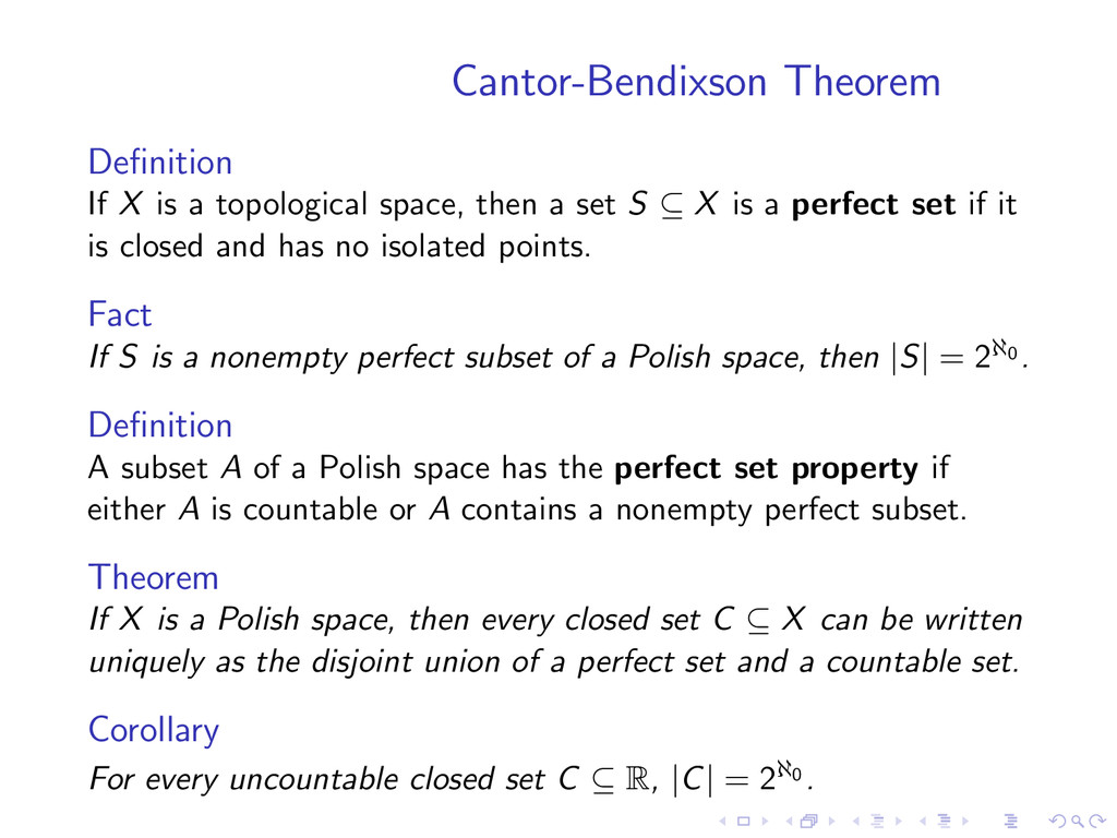
69. Cantor-Bendixson Theorem Definition If X is a topological space, then a set S ⊆ X is a perfect set if it is closed and has no isolated points. Fact If S is a nonempty perfect subset of a Polish space, then |S| = 2ℵ0 . Definition A subset A of a Polish space has the perfect set property if either A is countable or A contains a nonempty perfect subset. Theorem If X is a Polish space, then every closed set C ⊆ X can be written uniquely as the disjoint union of a perfect set and a countable set. Corollary For every uncountable closed set C ⊆ R, |C| = 2ℵ0 .
70. G˝ odel’s Constructible Universe The constructible universe, denoted L, was introduced by Kurt G˝ odel in 1938. It is a model of ZFC.
71. G˝ odel’s Constructible Universe The constructible universe, denoted L, was introduced by Kurt G˝ odel in 1938. It is a model of ZFC. L is, in a sense, the smallest model of ZFC containing all of the ordinals.
72. G˝ odel’s Constructible Universe The constructible universe, denoted L, was introduced by Kurt G˝ odel in 1938. It is a model of ZFC. L is, in a sense, the smallest model of ZFC containing all of the ordinals. CH is true in L.
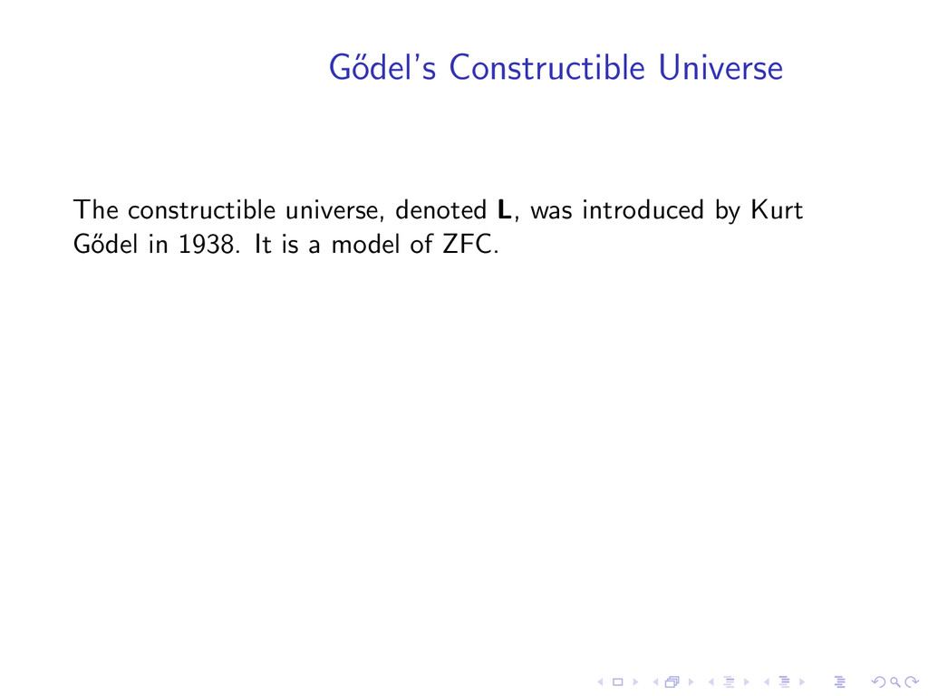
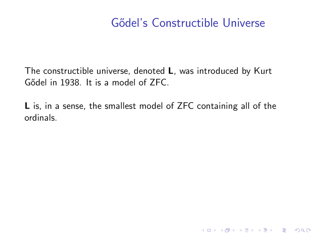
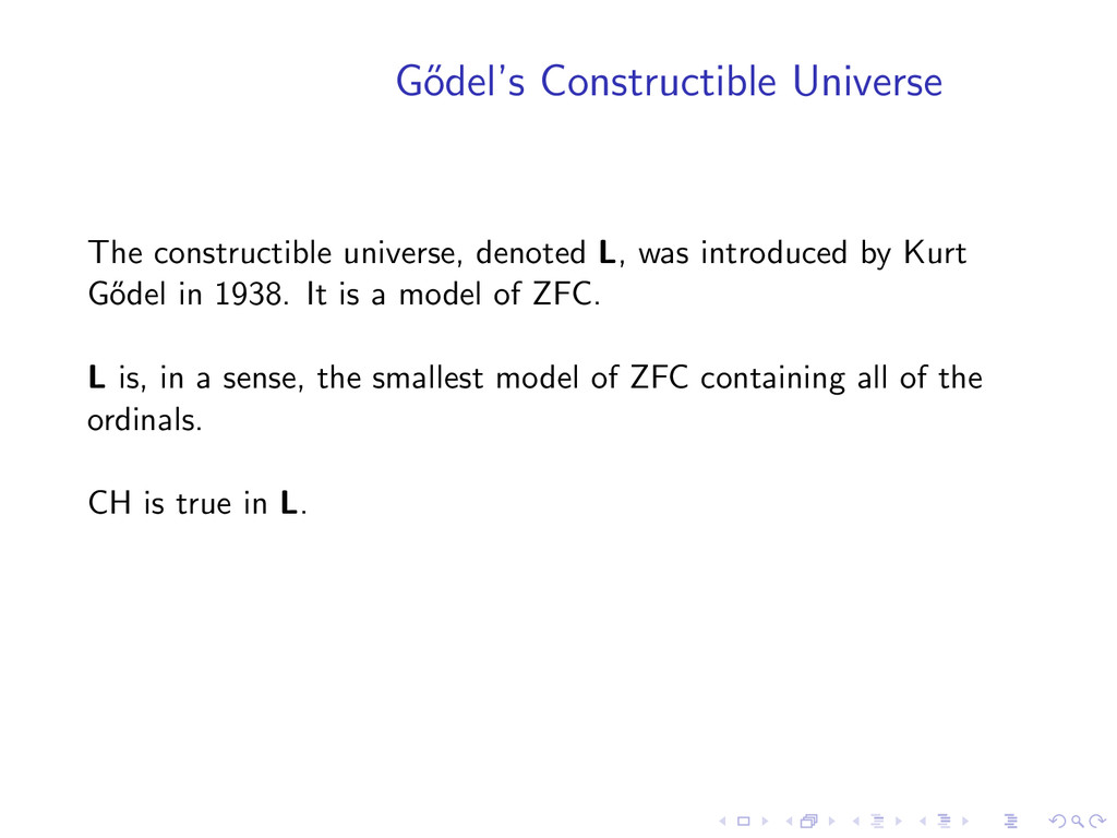
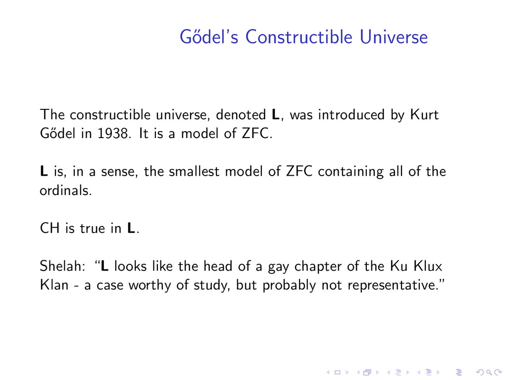
73. G˝ odel’s Constructible Universe The constructible universe, denoted L, was introduced by Kurt G˝ odel in 1938. It is a model of ZFC. L is, in a sense, the smallest model of ZFC containing all of the ordinals. CH is true in L. Shelah: “L looks like the head of a gay chapter of the Ku Klux Klan - a case worthy of study, but probably not representative.”
74. Forcing
75. Forcing In 1963, Paul Cohen introduced the technique of forcing, which allows for the construction of new models of ZFC.
76. Forcing In 1963, Paul Cohen introduced the technique of forcing, which allows for the construction of new models of ZFC. ”Adding sets, but very gently.”
77. Forcing In 1963, Paul Cohen introduced the technique of forcing, which allows for the construction of new models of ZFC. ”Adding sets, but very gently.” Cohen used forcing to construct a model of ZFC in which CH is false by adding ℵ2-many new subsets of ω.
78. Forcing In 1963, Paul Cohen introduced the technique of forcing, which allows for the construction of new models of ZFC. ”Adding sets, but very gently.” Cohen used forcing to construct a model of ZFC in which CH is false by adding ℵ2-many new subsets of ω. This “settled” Hilbert’s first problem.
79. The Axiom of Symmetry
80. The Axiom of Symmetry Let I = [0, 1], and let Iω denote the set of countable subsets of [0, 1].
81. The Axiom of Symmetry Let I = [0, 1], and let Iω denote the set of countable subsets of [0, 1]. AS: For every f : I → Iω, there are x, y ∈ I such that x ∈ f (y) and y ∈ f (x).
82. The Axiom of Symmetry Let I = [0, 1], and let Iω denote the set of countable subsets of [0, 1]. AS: For every f : I → Iω, there are x, y ∈ I such that x ∈ f (y) and y ∈ f (x). Lemma If CH is true, then AS is false.
83. The Axiom of Symmetry Let I = [0, 1], and let Iω denote the set of countable subsets of [0, 1]. AS: For every f : I → Iω, there are x, y ∈ I such that x ∈ f (y) and y ∈ f (x). Lemma If CH is true, then AS is false. Proof. Suppose CH is true and fix an enumeration of I: xα | α < ω1 .
84. The Axiom of Symmetry Let I = [0, 1], and let Iω denote the set of countable subsets of [0, 1]. AS: For every f : I → Iω, there are x, y ∈ I such that x ∈ f (y) and y ∈ f (x). Lemma If CH is true, then AS is false. Proof. Suppose CH is true and fix an enumeration of I: xα | α < ω1 . Define f : I → Iω by f (xα) = {xβ | β < α}.
85. The Axiom of Symmetry Let I = [0, 1], and let Iω denote the set of countable subsets of [0, 1]. AS: For every f : I → Iω, there are x, y ∈ I such that x ∈ f (y) and y ∈ f (x). Lemma If CH is true, then AS is false. Proof. Suppose CH is true and fix an enumeration of I: xα | α < ω1 . Define f : I → Iω by f (xα) = {xβ | β < α}. Then, for any α < β < ω1, xα ∈ f (xβ), so f is a counterexample to AS.
86. The Axiom of Symmetry AS is actually equivalent to the negation of CH and was introduced by Chris Freiling as an argument against CH.
87. The Axiom of Symmetry AS is actually equivalent to the negation of CH and was introduced by Chris Freiling as an argument against CH. Freiling’s Dartboard Argument:
88. The Axiom of Symmetry AS is actually equivalent to the negation of CH and was introduced by Chris Freiling as an argument against CH. Freiling’s Dartboard Argument: Fix an f : I → Iω.
89. The Axiom of Symmetry AS is actually equivalent to the negation of CH and was introduced by Chris Freiling as an argument against CH. Freiling’s Dartboard Argument: Fix an f : I → Iω. Throw two darts at the interval [0, 1].
90. The Axiom of Symmetry AS is actually equivalent to the negation of CH and was introduced by Chris Freiling as an argument against CH. Freiling’s Dartboard Argument: Fix an f : I → Iω. Throw two darts at the interval [0, 1]. If the first dart is thrown and lands at point x, then, since f (x) is countable and thus has measure 0, the probability that the second dart lands in f (x) is 0.
91. The Axiom of Symmetry AS is actually equivalent to the negation of CH and was introduced by Chris Freiling as an argument against CH. Freiling’s Dartboard Argument: Fix an f : I → Iω. Throw two darts at the interval [0, 1]. If the first dart is thrown and lands at point x, then, since f (x) is countable and thus has measure 0, the probability that the second dart lands in f (x) is 0. Since this is true no matter where the first dart lands, it should be true even before the first dart is thrown.
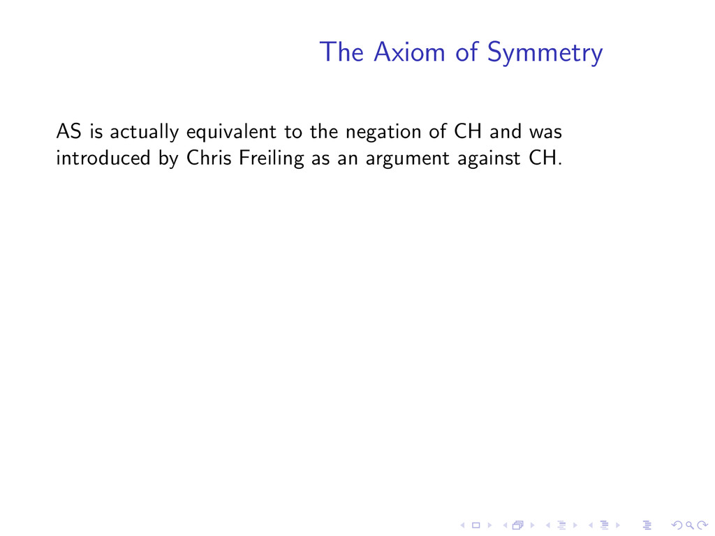
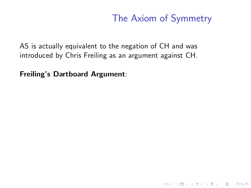
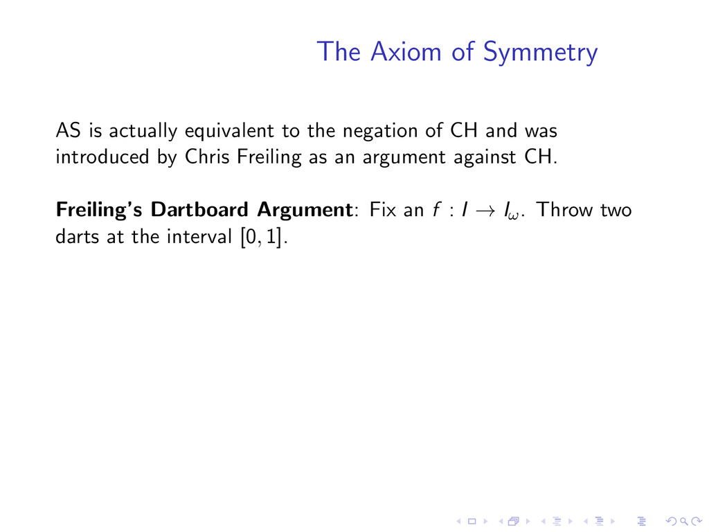
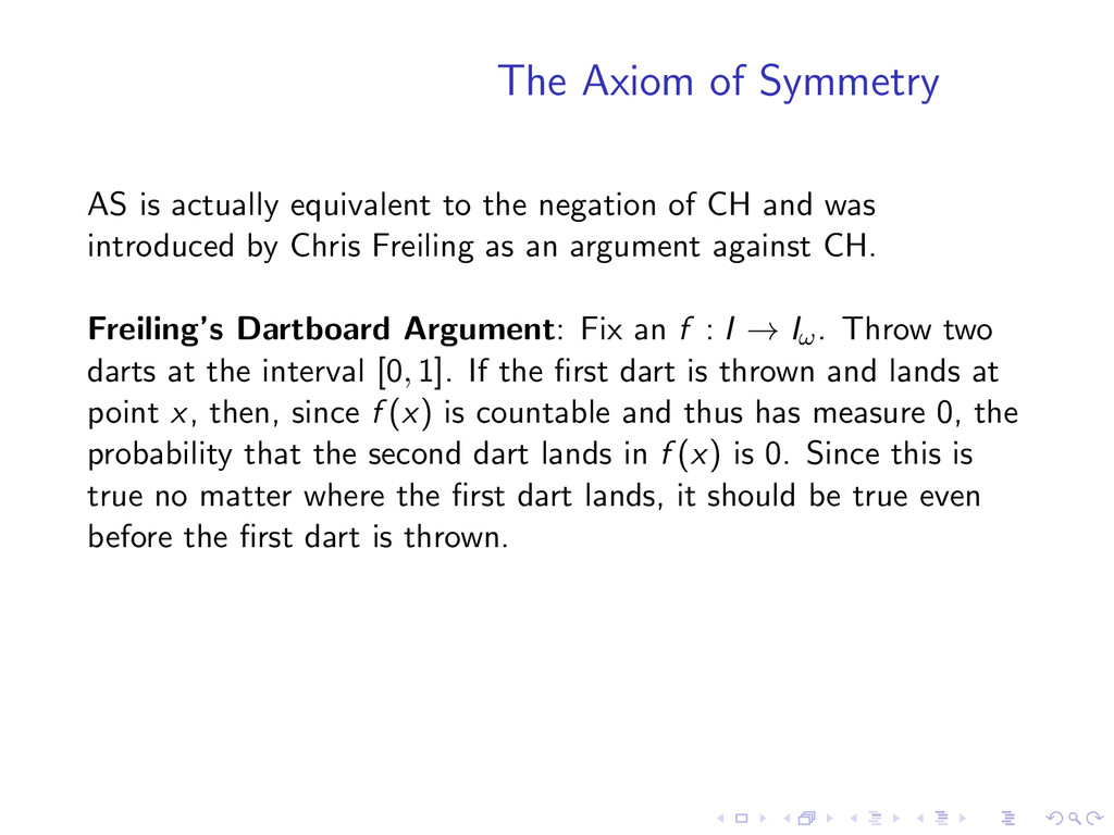
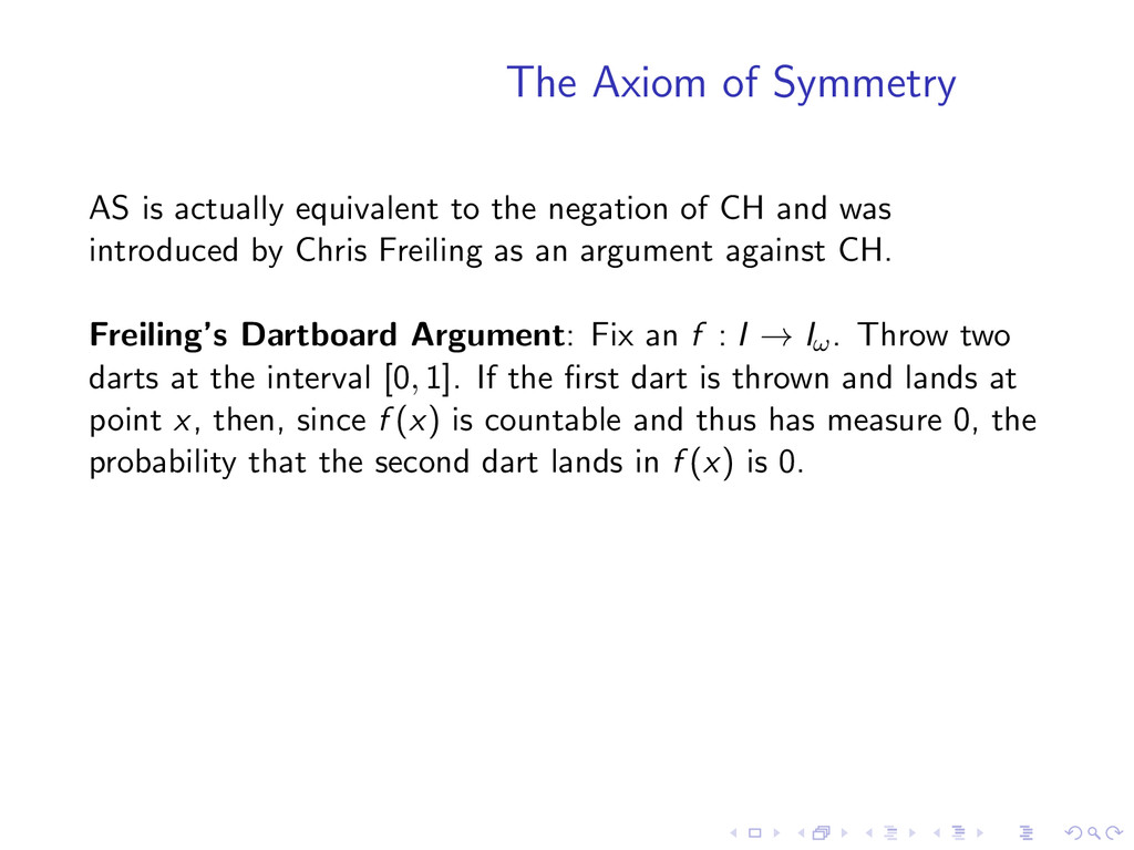
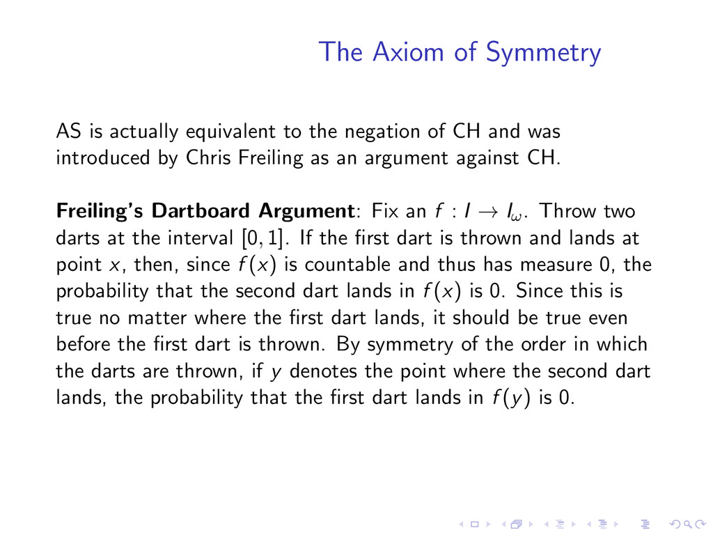
92. The Axiom of Symmetry AS is actually equivalent to the negation of CH and was introduced by Chris Freiling as an argument against CH. Freiling’s Dartboard Argument: Fix an f : I → Iω. Throw two darts at the interval [0, 1]. If the first dart is thrown and lands at point x, then, since f (x) is countable and thus has measure 0, the probability that the second dart lands in f (x) is 0. Since this is true no matter where the first dart lands, it should be true even before the first dart is thrown. By symmetry of the order in which the darts are thrown, if y denotes the point where the second dart lands, the probability that the first dart lands in f (y) is 0.
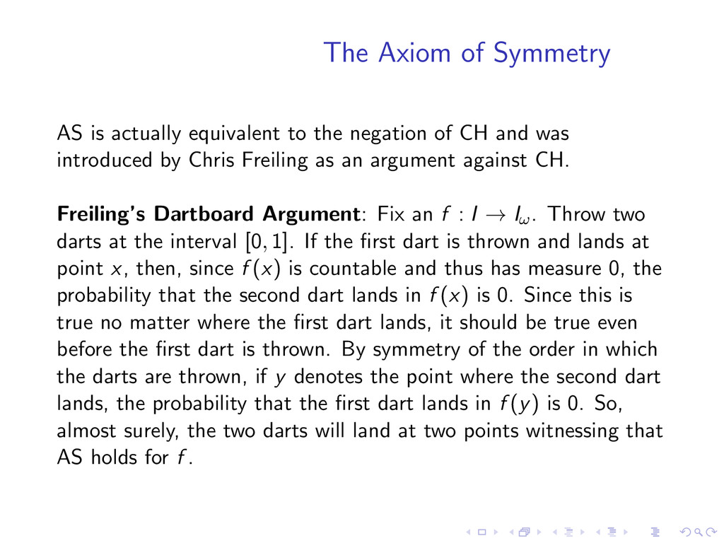
93. The Axiom of Symmetry AS is actually equivalent to the negation of CH and was introduced by Chris Freiling as an argument against CH. Freiling’s Dartboard Argument: Fix an f : I → Iω. Throw two darts at the interval [0, 1]. If the first dart is thrown and lands at point x, then, since f (x) is countable and thus has measure 0, the probability that the second dart lands in f (x) is 0. Since this is true no matter where the first dart lands, it should be true even before the first dart is thrown. By symmetry of the order in which the darts are thrown, if y denotes the point where the second dart lands, the probability that the first dart lands in f (y) is 0. So, almost surely, the two darts will land at two points witnessing that AS holds for f .
94. Problems with Freiling’s Arguments Two main objections can be raised.
95. Problems with Freiling’s Arguments Two main objections can be raised. One objection involves Lebesgue measurability:
96. Problems with Freiling’s Arguments Two main objections can be raised. One objection involves Lebesgue measurability: Freiling’s argument seems to appeal to an intuition that {(x, y) | x ∈ f (y)} and {(x, y) | y ∈ f (x)} both have measure 0.
97. Problems with Freiling’s Arguments Two main objections can be raised. One objection involves Lebesgue measurability: Freiling’s argument seems to appeal to an intuition that {(x, y) | x ∈ f (y)} and {(x, y) | y ∈ f (x)} both have measure 0. This intuition seems to require that there is a very well-behaved measure on the reals, which is precluded by the Axiom of Choice.
98. Problems with Freiling’s Arguments Two main objections can be raised. One objection involves Lebesgue measurability: Freiling’s argument seems to appeal to an intuition that {(x, y) | x ∈ f (y)} and {(x, y) | y ∈ f (x)} both have measure 0. This intuition seems to require that there is a very well-behaved measure on the reals, which is precluded by the Axiom of Choice. In fact, if f is a counterexample to AS, then both {(x, y) | x ∈ f (y)} and {(x, y) | y ∈ f (x)} are non-measurable.
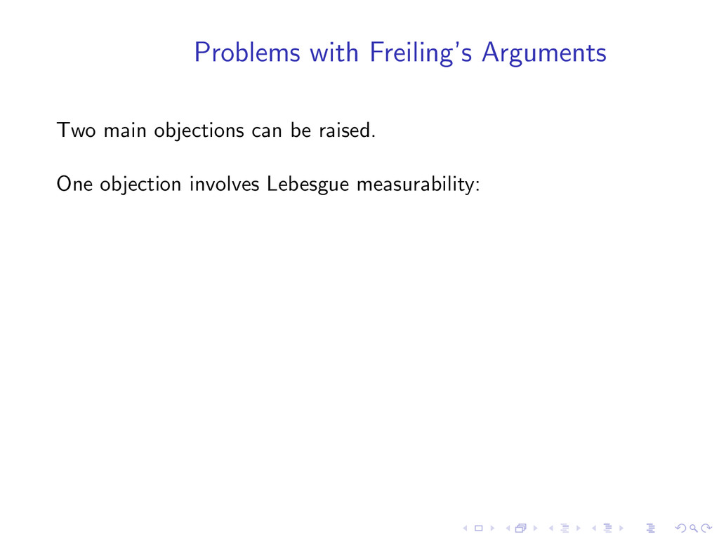
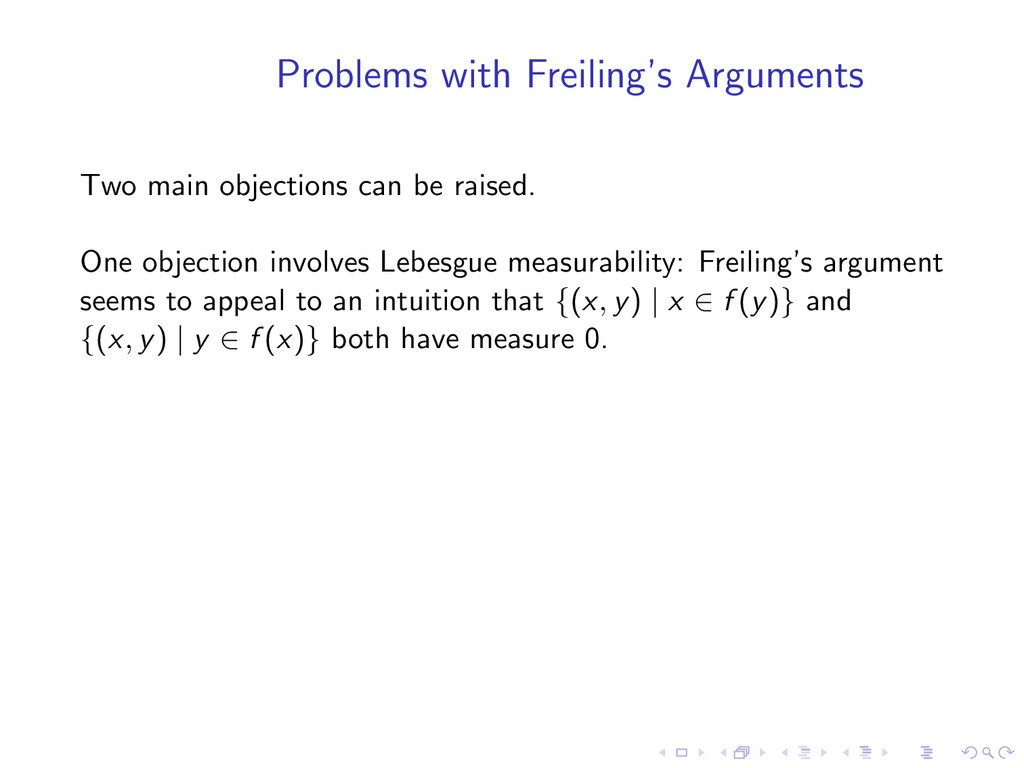
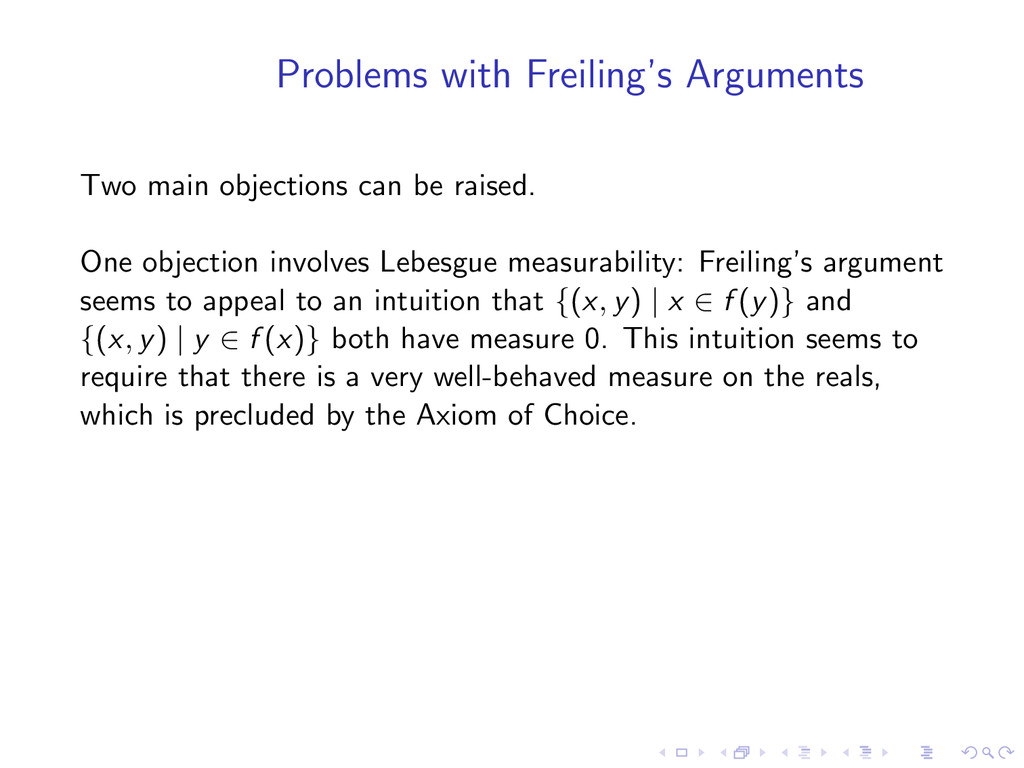
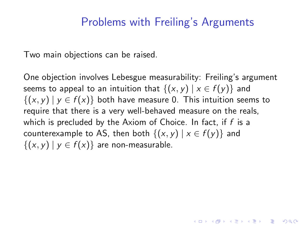
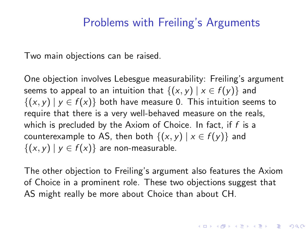
99. Problems with Freiling’s Arguments Two main objections can be raised. One objection involves Lebesgue measurability: Freiling’s argument seems to appeal to an intuition that {(x, y) | x ∈ f (y)} and {(x, y) | y ∈ f (x)} both have measure 0. This intuition seems to require that there is a very well-behaved measure on the reals, which is precluded by the Axiom of Choice. In fact, if f is a counterexample to AS, then both {(x, y) | x ∈ f (y)} and {(x, y) | y ∈ f (x)} are non-measurable. The other objection to Freiling’s argument also features the Axiom of Choice in a prominent role.
100. Problems with Freiling’s Arguments Two main objections can be raised. One objection involves Lebesgue measurability: Freiling’s argument seems to appeal to an intuition that {(x, y) | x ∈ f (y)} and {(x, y) | y ∈ f (x)} both have measure 0. This intuition seems to require that there is a very well-behaved measure on the reals, which is precluded by the Axiom of Choice. In fact, if f is a counterexample to AS, then both {(x, y) | x ∈ f (y)} and {(x, y) | y ∈ f (x)} are non-measurable. The other objection to Freiling’s argument also features the Axiom of Choice in a prominent role. These two objections suggest that AS might really be more about Choice than about CH.
101. Solovay’s Model Soon after Cohen introduced it, Solovay used the technique of forcing to construct a model S of ZF + DC in which:
102. Solovay’s Model Soon after Cohen introduced it, Solovay used the technique of forcing to construct a model S of ZF + DC in which: 1 All sets of real numbers are Lebesgue measurable.
103. Solovay’s Model Soon after Cohen introduced it, Solovay used the technique of forcing to construct a model S of ZF + DC in which: 1 All sets of real numbers are Lebesgue measurable. 2 All sets of real numbers have the perfect set property.
104. Solovay’s Model Soon after Cohen introduced it, Solovay used the technique of forcing to construct a model S of ZF + DC in which: 1 All sets of real numbers are Lebesgue measurable. 2 All sets of real numbers have the perfect set property. The existence of an injective function f : ω1 → R is enough to construct a non-measurable set, so, in S, ℵ1 and 2ℵ0 are not even comparable.
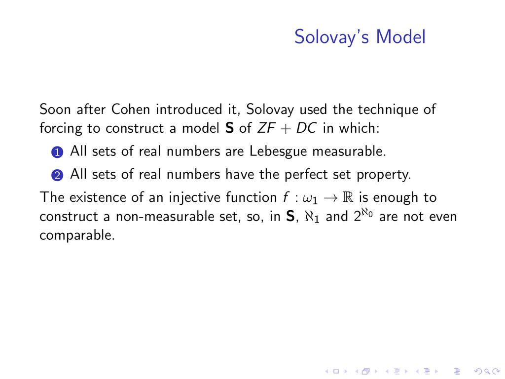
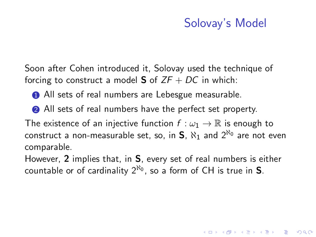
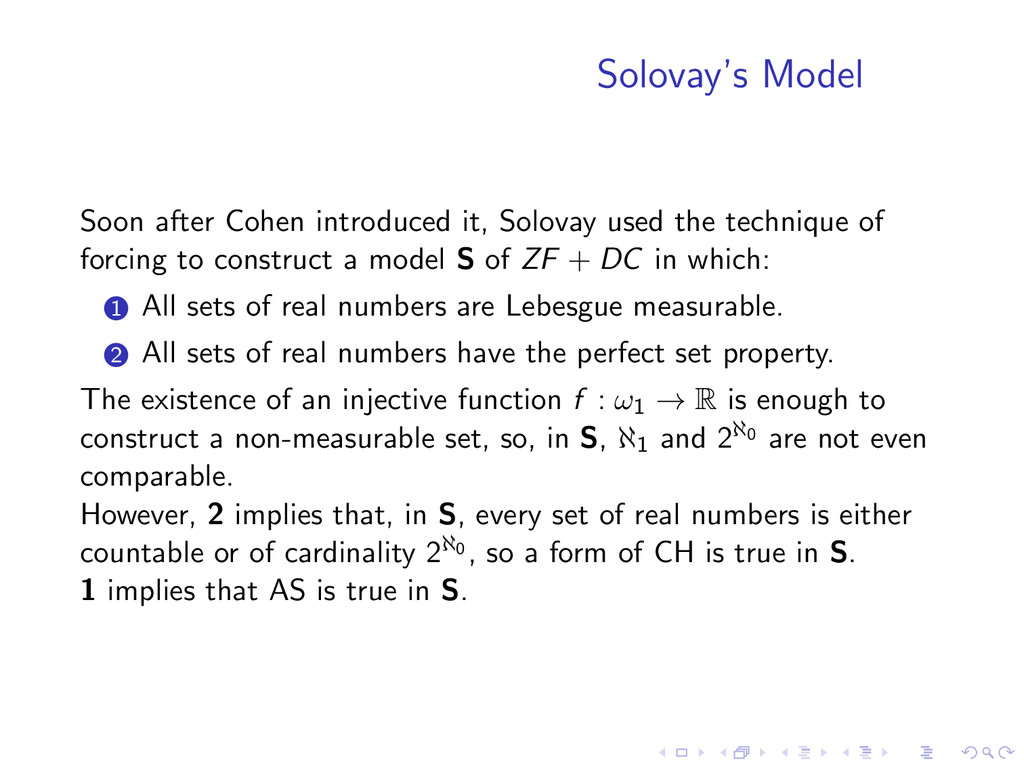
105. Solovay’s Model Soon after Cohen introduced it, Solovay used the technique of forcing to construct a model S of ZF + DC in which: 1 All sets of real numbers are Lebesgue measurable. 2 All sets of real numbers have the perfect set property. The existence of an injective function f : ω1 → R is enough to construct a non-measurable set, so, in S, ℵ1 and 2ℵ0 are not even comparable. However, 2 implies that, in S, every set of real numbers is either countable or of cardinality 2ℵ0 , so a form of CH is true in S.
106. Solovay’s Model Soon after Cohen introduced it, Solovay used the technique of forcing to construct a model S of ZF + DC in which: 1 All sets of real numbers are Lebesgue measurable. 2 All sets of real numbers have the perfect set property. The existence of an injective function f : ω1 → R is enough to construct a non-measurable set, so, in S, ℵ1 and 2ℵ0 are not even comparable. However, 2 implies that, in S, every set of real numbers is either countable or of cardinality 2ℵ0 , so a form of CH is true in S. 1 implies that AS is true in S.
107. Closing Remarks