Upgrade to Pro — share decks privately, control downloads, hide ads and more …

Sensitivity Analysis of a Bottom Reflood Simulation using the Morris Screening Method

Damar Wicaksono
December 17, 2014

Sensitivity Analysis of a Bottom Reflood Simulation using the Morris Screening Method

(Presented at the 10th International Topical Meeting on Nuclear Reactor Thermal Hydraulics, Operation and Safety NUTHOS-10, Okinawa, Japan, 2014)

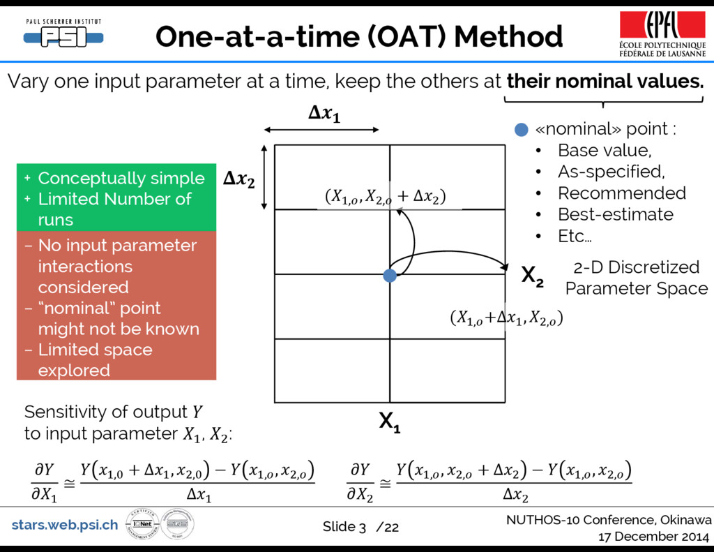
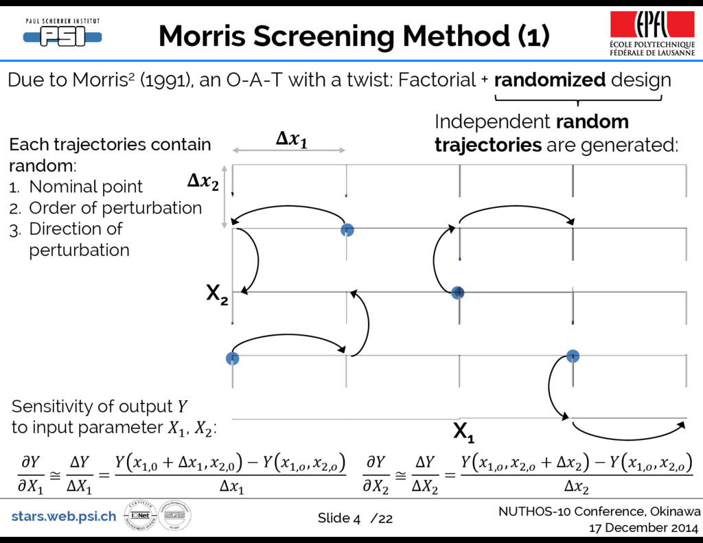
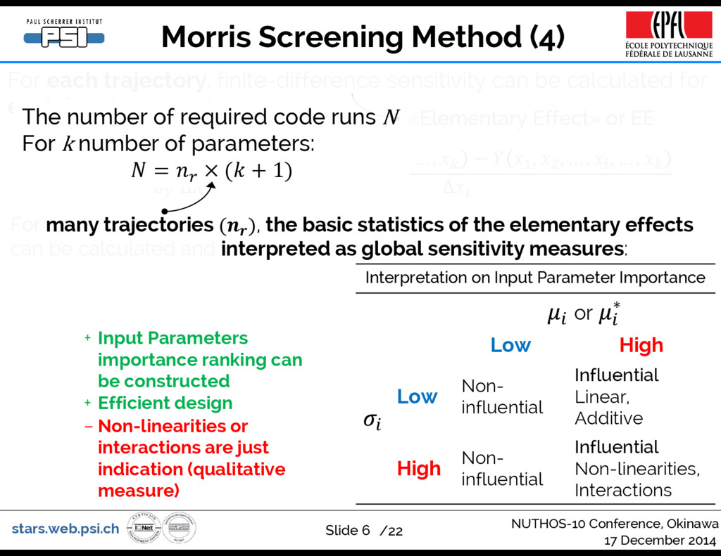
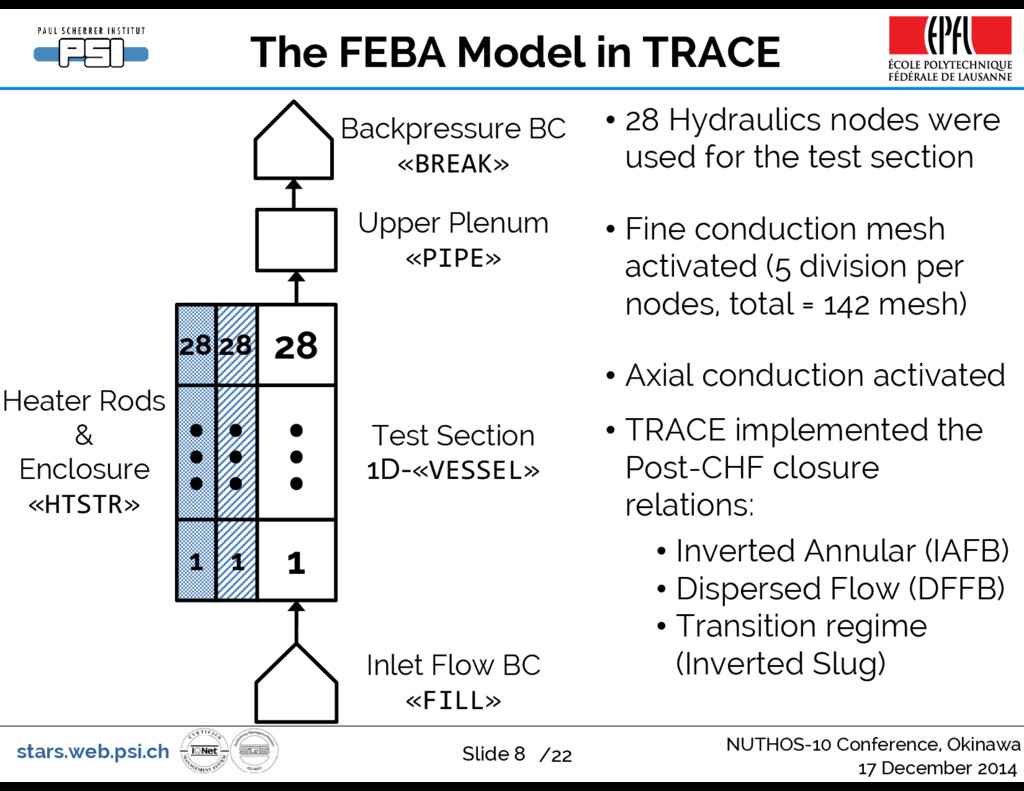
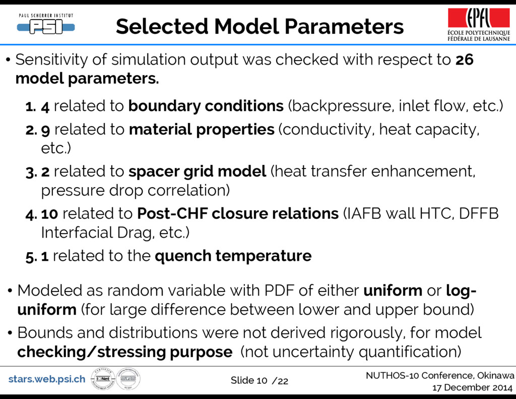
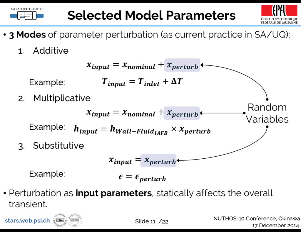
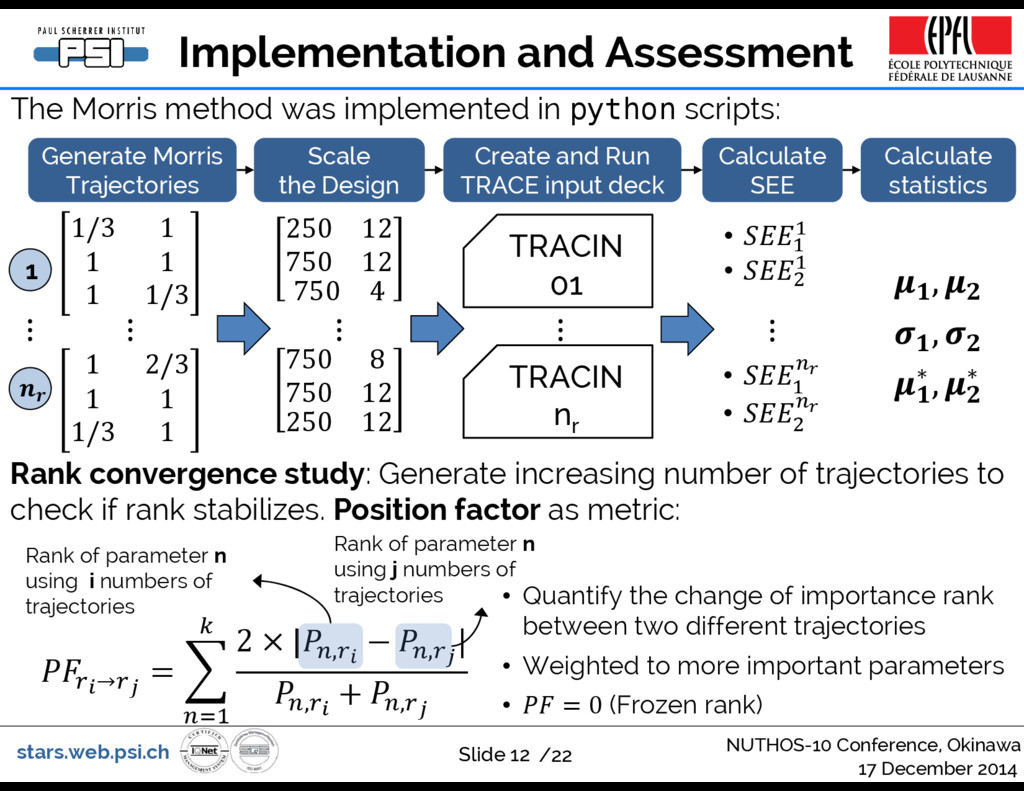
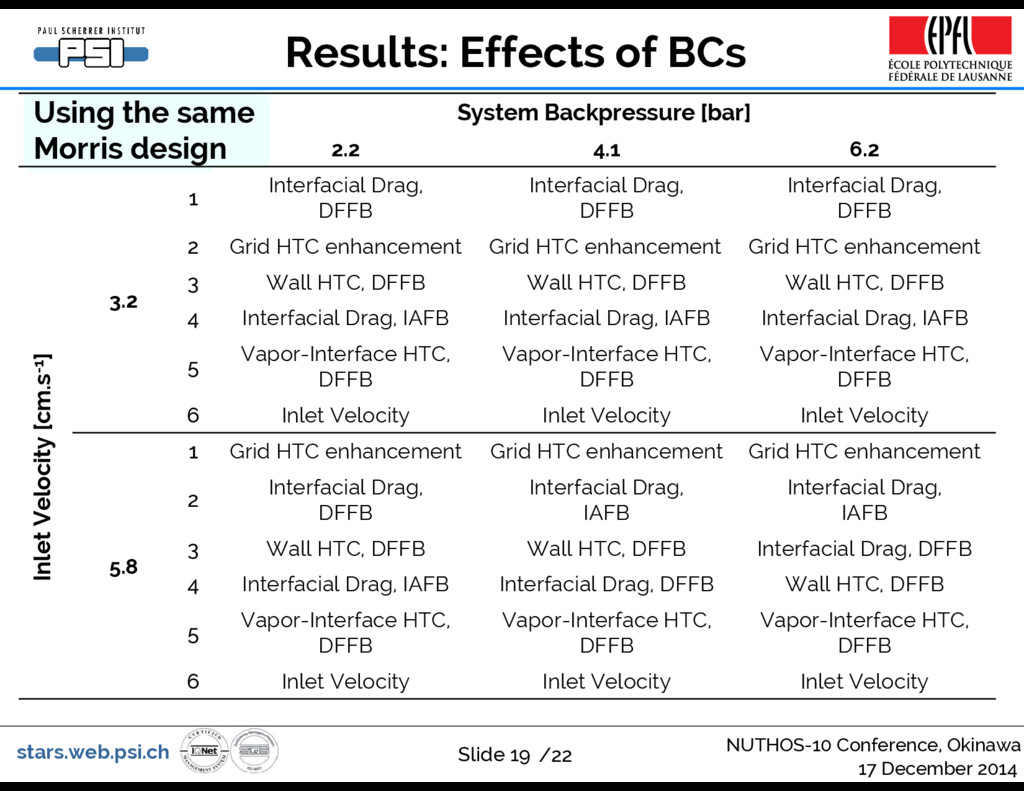
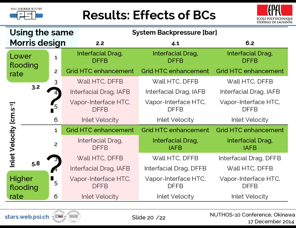
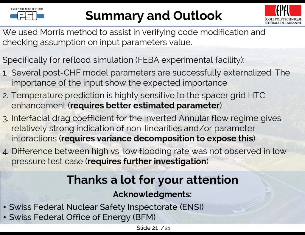
Simulation of reflood phase during loss-of-coolant accident in a nuclear reactor power plant is an important part in the plant safety analysis. During reflood, a steady stream of water is injected into a dry fuel channel to cool down the heated channel and to prevent fuel damage due to overheating. Computer simulation of such phenomena relied on a set of phenomenological models that contains uncertain parameters. The importance of these parameters to the quantity of interest in the prediction, such as the maximum fuel temperature prediction, is usually not known a priori. This talk will explain the use of statistical method for model sensitivity analysis called the Morris screening method to identify the most important parameters relevant to the prediction of the quantity of interest. Such identification is important for preliminary verification and validation of the model (e.g., in confirming certain expectation about parameters importance) as well as for possible simplification of the model (e.g., removing redundant parameter in downstream analysis).
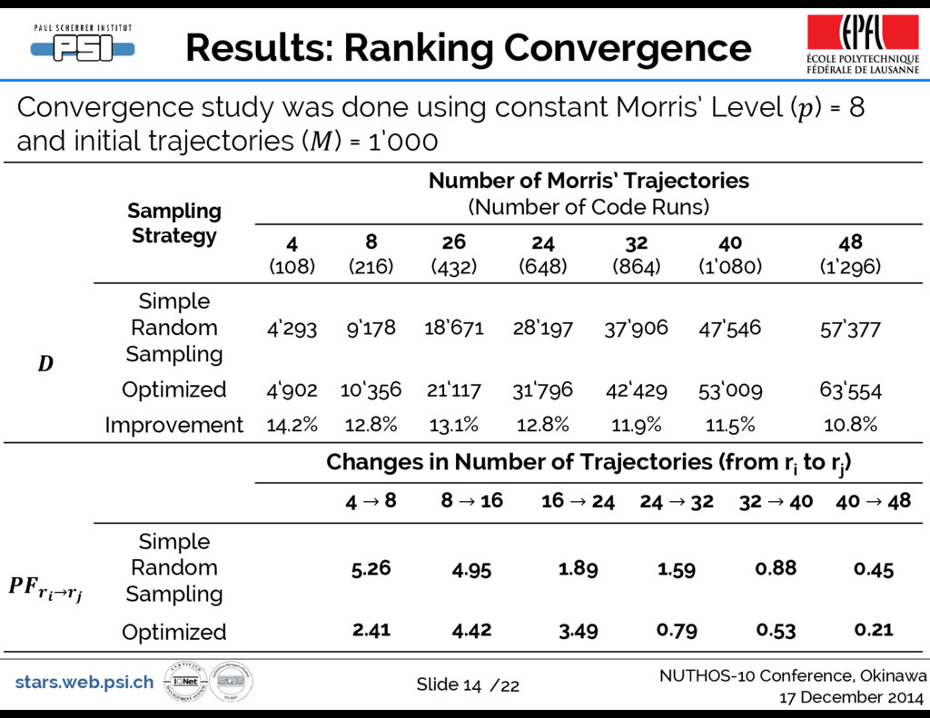
Damar Wicaksono

December 17, 2014
Tweet

More Decks by Damar Wicaksono

Other Decks in Science

Transcript

  1. Wir schaffen Wissen – heute für morgen Laboratory for Reactor

    Physics and Systems Behaviour (LRS) NUTHOS-10 Conference, Okinawa, Japan 17th December 2014 Sensitivity Analysis of a Bottom Reflood Simulation using the Morris Screening Method D. Wicaksono, O. Zerkak, and A. Pautz
  2. stars.web.psi.ch /22 Background and Motivation Slide 2 Use sentivity analysis

    method as a preliminary model checking / assessment tool. Specifically: 1. To check if model behaves as expected as input varies 2. To identify the importance of parameters to the model output 3. To identify which parameters need to be better estimated Preliminary: computationally cheap method but better than quick and dirty 17 December 2014 NUTHOS-10 Conference, Okinawa During the work for PSI contribution to the OECD/NEA PREMIUM Phase III Modeling of FEBA separate effect test in TRACE1 code based on the benchmark specification. 1. TRACE requires some specific input, not known, requires assumptions (needs checking) 2. TRACE v5.0p3 was modified to allow access to important model parameters at input deck level (needs verification) Adopted approach:
  3. stars.web.psi.ch /22 One-at-a-time (OAT) Method Slide 3 Vary one input

    parameter at a time, keep the others at their nominal values. 2-D Discretized Parameter Space «nominal» point : • Base value, • As-specified, • Recommended • Best-estimate • Etc… X1 , , , Δ , Δ , , ≅ , Δ , , , , , Δ ≅ , , , Δ , , , Δ X2 Sensitivity of output to input parameter , : + Conceptually simple + Limited Number of runs − No input parameter interactions considered − “nominal” point might not be known − Limited space explored 17 December 2014 NUTHOS-10 Conference, Okinawa
  4. stars.web.psi.ch /22 Morris Screening Method (1) Slide 4 Due to

    Morris2 (1991), an O-A-T with a twist: Factorial + randomized design X1 Each trajectories contain random: 1. Nominal point 2. Order of perturbation 3. Direction of perturbation ≅ Δ Δ , Δ , , , , , Δ ≅ Δ Δ , , , Δ , , , Δ X2 Sensitivity of output to input parameter , : Independent random trajectories are generated: 17 December 2014 NUTHOS-10 Conference, Okinawa
  5. stars.web.psi.ch /22 Morris Screening Method (2) Slide 5 For each

    trajectory, finite-difference sensitivity can be calculated for each input parameter: ≡ Δ Δ , , … , Δ , … , , , … , , … , Δ For many trajectories , the basic statistics of the elementary effects can be calculated and interpreted as global sensitivity measures: «Elementary Effect» or EE Mean 1 Standard Deviation 1 Mean of Absolute Value3 ∗ 1 | | Interpretation on Input Parameter Importance or ∗ Low High Low Non- influential Influential Linear, Additive High Non- influential Influential Non-linearities, Interactions 17 December 2014 NUTHOS-10 Conference, Okinawa
  6. stars.web.psi.ch /22 Morris Screening Method (4) Slide 6 For each

    trajectory, finite-difference sensitivity can be calculated for each input parameter: ≡ Δ Δ , , … , Δ , … , , , … , , … , Δ For many trajectories , the basic statistics of the elementary effects can be calculated and interpreted as global sensitivity measures: «Elementary Effect» or EE + Input Parameters importance ranking can be constructed + Efficient design − Non-linearities or interactions are just indication (qualitative measure) Interpretation on Input Parameter Importance or ∗ Low High Low Non- influential Influential Linear, Additive High Non- influential Influential Non-linearities, Interactions 17 December 2014 NUTHOS-10 Conference, Okinawa The number of required code runs N For k number of parameters: 1
  7. stars.web.psi.ch /22 The FEBA Facility Slide 7 • FEBA Reflood

    Test was conducted at Karlsruhe Institute of Technology during 1980s for investigating bottom reflood heat transfer and codes validation (Spec. & Data Publicly Available5) • Full height (4.114 [m]) 5x5 PWR Rod Bundle with 7 spacer grids FEBA Rod Simulator FEBA Bundle Top View (5x5 Rod Bundle) Approximate Cosine Power Profile All dimensions in [mm] Nominal Power: 120% ANS Decay Heat 17 December 2014 NUTHOS-10 Conference, Okinawa
  8. stars.web.psi.ch /22 The FEBA Model in TRACE Slide 8 1

    28 1 1 28 28 Backpressure BC «BREAK» Upper Plenum «PIPE» Test Section 1D-«VESSEL» Inlet Flow BC «FILL» Heater Rods & Enclosure «HTSTR» 17 December 2014 NUTHOS-10 Conference, Okinawa • 28 Hydraulics nodes were used for the test section • Fine conduction mesh activated (5 division per nodes, total = 142 mesh) • Axial conduction activated • TRACE implemented the Post-CHF closure relations: • Inverted Annular (IAFB) • Dispersed Flow (DFFB) • Transition regime (Inverted Slug)
  9. stars.web.psi.ch /22 The FEBA Model in TRACE Slide 9 17

    December 2014 NUTHOS-10 Conference, Okinawa • 28 Hydraulics nodes were used for the test section • Fine conduction mesh activated (5 division per nodes, total = 142 mesh) • Axial conduction activated • TRACE implemented the Post-CHF closure relations: • Inverted Annular (IAFB) • Dispersed Flow (DFFB) • Transition regime (Inverted Slug) Bottom Reflood Phenomenology in TRACE1
  10. stars.web.psi.ch /22 Selected Model Parameters Slide 10 17 December 2014

    NUTHOS-10 Conference, Okinawa • Sensitivity of simulation output was checked with respect to 26 model parameters. 1. 4 related to boundary conditions (backpressure, inlet flow, etc.) 2. 9 related to material properties (conductivity, heat capacity, etc.) 3. 2 related to spacer grid model (heat transfer enhancement, pressure drop correlation) 4. 10 related to Post-CHF closure relations (IAFB wall HTC, DFFB Interfacial Drag, etc.) 5. 1 related to the quench temperature • Modeled as random variable with PDF of either uniform or log- uniform (for large difference between lower and upper bound) • Bounds and distributions were not derived rigorously, for model checking/stressing purpose (not uncertainty quantification)
  11. stars.web.psi.ch /22 Selected Model Parameters Slide 11 17 December 2014

    NUTHOS-10 Conference, Okinawa • 3 Modes of parameter perturbation (as current practice in SA/UQ): 1. Additive 2. Multiplicative 3. Substitutive • Perturbation as input parameters, statically affects the overall transient. Random Variables Example: Example: Example:
  12. stars.web.psi.ch /22 Implementation and Assessment Slide 12 The Morris method

    was implemented in python scripts: Generate Morris Trajectories Scale the Design Create and Run TRACE input deck Calculate statistics Rank convergence study: Generate increasing number of trajectories to check if rank stabilizes. Position factor as metric: → 2 | , , | , , • Quantify the change of importance rank between two different trajectories • Weighted to more important parameters • 0 (Frozen rank) Rank of parameter n using i numbers of trajectories Rank of parameter n using j numbers of trajectories 750 8 750 12 250 12 ∗ ∗ TRACIN 01 TRACIN nr 1 2/3 1 1 1/3 1 1/3 1 1 1 1 1/3 250 12 750 12 750 4 1 Calculate SEE • • • • 17 December 2014 NUTHOS-10 Conference, Okinawa
  13. stars.web.psi.ch /22 Sampling Strategy Slide 13 [3] Asserted parameter space

    coverage is important, each grid points in the parameter space needs to be sampled evenly. (Better design covers more space). For a given number of required trajectories, maximize the total distance between pair of trajectories from a large number of initial trajectories (M). Distance between two trajectories is defined by: 17 December 2014 NUTHOS-10 Conference, Okinawa basic Function Morris Method : Trajectoty[1000] - Level [4] Replica 1000 x3 0 0.2 0.4 0.6 0.8 1 x2 0 0.2 0.4 0.6 0.8 1 x1 0 0.2 0.4 0.6 0.8 1 x1:x2:x3 Number of selected Trajectories M = 1000 5 10 20 Evaluations 8.25 10 2.63 10 3.39 10 We follow heuristic optimization scheme proposed in [4], with complexity . .
  14. stars.web.psi.ch /22 Results: Ranking Convergence Slide 14 Sampling Strategy Number

    of Morris’ Trajectories (Number of Code Runs) 4 (108) 8 (216) 26 (432) 24 (648) 32 (864) 40 (1’080) 48 (1’296) Simple Random Sampling 4’293 9’178 18’671 28’197 37’906 47’546 57’377 Optimized 4‘902 10‘356 21‘117 31‘796 42‘429 53‘009 63‘554 Improvement 14.2% 12.8% 13.1% 12.8% 11.9% 11.5% 10.8% Changes in Number of Trajectories (from ri to rj ) 4 → 8 8 → 16 16 → 24 24 → 32 32 → 40 40 → 48 → Simple Random Sampling 5.26 4.95 1.89 1.59 0.88 0.45 Optimized 2.41 4.42 3.49 0.79 0.53 0.21 Convergence study was done using constant Morris’ Level ( ) = 8 and initial trajectories ( ) = 1’000 17 December 2014 NUTHOS-10 Conference, Okinawa
  15. stars.web.psi.ch /22 Results: Ranking Convergence Slide 15 Sampling Strategy Number

    of Morris’ Trajectories (Number of Code Runs) 4 (108) 8 (216) 26 (432) 24 (648) 32 (864) 40 (1’080) 48 (1’296) Simple Random Sampling 4’293 9’178 18’671 28’197 37’906 47’546 57’377 Optimized 4‘902 10‘356 21‘117 31‘796 42‘429 53‘009 63‘554 Improvement 14.2% 12.8% 13.1% 12.8% 11.9% 11.5% 10.8% Changes in Number of Trajectories (from ri to rj ) 4 → 8 8 → 16 16 → 24 24 → 32 32 → 40 40 → 48 → Simple Random Sampling 5.26 4.95 1.89 1.59 0.88 0.45 Optimized 2.41 4.42 3.49 0.79 0.53 0.21 Convergence study was done using (optimized scheme: use initial trajectories ( ) = 1’000) Modest gain in coverage Rank stabilized with fewer code runs 17 December 2014 NUTHOS-10 Conference, Okinawa
  16. stars.web.psi.ch /22 Results: Screening (1) Slide 16 17 December 2014

    NUTHOS-10 Conference, Okinawa ∗ 2 The Morris plot shown for vs. ∗exposes parameters importance ranking at a glance (regardless of their signed effect) √ (comparing of the size of mean and std. deviation) Standard Error of the Mean At Mid-Assembly (Test 216) Wall HTC (Dispersed Flow) Spacer Grid HTC Enhancement Inlet velocity Vapor-Interface HTC (Dispersed Flow) Interfacial Drag (Inverted Annular) Interfacial Drag (Dispersed Flow) 6 Most influential parameters: 1.Interfacial Drag, DFFB 2.Spacer Grid HTC Enhancement 3.Wall HTC, DFFB 4.Interfacial Drag, IAFB 5.Vapor-Interface HTC, DFFB 6.Inlet velocity Strong non-linearities and/or interactions
  17. stars.web.psi.ch /22 Results: Screening (2) Slide 17 17 December 2014

    NUTHOS-10 Conference, Okinawa ∗ At Mid-Assembly (Test 216) 5 least influential parameters: 1. Conductivity, rod bundle enclosure 2. Wall Drag, IAFB 3. Emissivity, cladding 4. Conductivity, cladding 5. Wall roughness Strong non-linearities and/or interactions Non-influential parameters are the ones with small (clustered at the origin)
  18. stars.web.psi.ch /22 Results: Screening (3) Slide 18 17 December 2014

    NUTHOS-10 Conference, Okinawa We expect certain things: 1. Forced reflood should be dominated by Post-CHF mechanisms. Hydrodynamic-related parameter of these flow regimes are indeed important (Interfacial Drag for DFFB and IFFB). 2. For low flooding rate, DFFB should dominate the process. 3. Material properties bounds are as specified by the benchmark/databank (and rather narrow). But, there are some additional findings: 1. Spacer grid convective heat transfer enhancement has very strong effect on temperature prediction. Exclude (for conservatism?) or properly specified if included. 2. None of the parameters are strongly non-linear or interacting. Interfacial drag for IAFB has, relatively, the strongest of either of these effects for the temperature prediction. Morris couldn’t tell how exactly (variance decomposition method?)
  19. stars.web.psi.ch /22 Results: Effects of BCs Slide 19 17 December

    2014 NUTHOS-10 Conference, Okinawa System Backpressure [bar] 2.2 4.1 6.2 3.2 1 Interfacial Drag, DFFB Interfacial Drag, DFFB Interfacial Drag, DFFB 2 Grid HTC enhancement Grid HTC enhancement Grid HTC enhancement 3 Wall HTC, DFFB Wall HTC, DFFB Wall HTC, DFFB 4 Interfacial Drag, IAFB Interfacial Drag, IAFB Interfacial Drag, IAFB 5 Vapor-Interface HTC, DFFB Vapor-Interface HTC, DFFB Vapor-Interface HTC, DFFB 6 Inlet Velocity Inlet Velocity Inlet Velocity 5.8 1 Grid HTC enhancement Grid HTC enhancement Grid HTC enhancement 2 Interfacial Drag, DFFB Interfacial Drag, IAFB Interfacial Drag, IAFB 3 Wall HTC, DFFB Wall HTC, DFFB Interfacial Drag, DFFB 4 Interfacial Drag, IAFB Interfacial Drag, DFFB Wall HTC, DFFB 5 Vapor-Interface HTC, DFFB Vapor-Interface HTC, DFFB Vapor-Interface HTC, DFFB 6 Inlet Velocity Inlet Velocity Inlet Velocity Using the same Morris design Inlet Velocity [cm.s-1]
  20. stars.web.psi.ch /22 Results: Effects of BCs Slide 20 17 December

    2014 NUTHOS-10 Conference, Okinawa System Backpressure [bar] 2.2 4.1 6.2 3.2 1 Interfacial Drag, DFFB Interfacial Drag, DFFB Interfacial Drag, DFFB 2 Grid HTC enhancement Grid HTC enhancement Grid HTC enhancement 3 Wall HTC, DFFB Wall HTC, DFFB Wall HTC, DFFB 4 Interfacial Drag, IAFB Interfacial Drag, IAFB Interfacial Drag, IAFB 5 Vapor-Interface HTC, DFFB Vapor-Interface HTC, DFFB Vapor-Interface HTC, DFFB 6 Inlet Velocity Inlet Velocity Inlet Velocity 5.8 1 Grid HTC enhancement Grid HTC enhancement Grid HTC enhancement 2 Interfacial Drag, DFFB Interfacial Drag, IAFB Interfacial Drag, IAFB 3 Wall HTC, DFFB Wall HTC, DFFB Interfacial Drag, DFFB 4 Interfacial Drag, IAFB Interfacial Drag, DFFB Wall HTC, DFFB 5 Vapor-Interface HTC, DFFB Vapor-Interface HTC, DFFB Vapor-Interface HTC, DFFB 6 Inlet Velocity Inlet Velocity Inlet Velocity Using the same Morris design Inlet Velocity [cm.s-1] Lower flooding rate Higher flooding rate ? ?
  21. /21 Summary and Outlook Slide 21 Thanks a lot for

    your attention Acknowledgments: • Swiss Federal Nuclear Safety Inspectorate (ENSI) • Swiss Federal Office of Energy (BFM) We used Morris method to assist in verifying code modification and checking assumption on input parameters value. Specifically for reflood simulation (FEBA experimental facility): 1. Several post-CHF model parameters are successfully externalized. The importance of the input show the expected importance 2. Temperature prediction is highly sensitive to the spacer grid HTC enhancement (requires better estimated parameter) 3. Interfacial drag coefficient for the Inverted Annular flow regime gives relatively strong indication of non-linearities and/or parameter interactions (requires variance decomposition to expose this) 4. Difference between high vs. low flooding rate was not observed in low pressure test case (requires further investigation)
  22. stars.web.psi.ch /22 References 1 United States Nuclear Regulatory Commission (US

    N.R.C.), “TRACE v5.0p3 Theory Manual,” 2012. 2 M. D. Morris, “Factorial Sampling Plans for Preliminary Computational Experiments,” Technometrics,vol. 33, no. 2, pp. 161 – 174, 1991. 3 F. Campolongo, J. Cariboni, and A. Saltelli, “An effective screening design for sensitivity analysis for large models,” Environmental Modelling & Software, vol. 22, pp. 1509 – 1518, 2007. 4 M. V. Ruano, J. Ribes, A. Seco, and J. Ferrer, “An Improved Sampling Strategy based on Trajectory Design for Application of the Morris Method to Systems with Many Input Factors,” Environmental Modelling & Software, vol. 37, pp. 103 – 109, 2012. 5 P. Ihle and K. Rust, “FEBA-Flooding Experiments with Blocked Arrays: Evaluation Report,” Kernforschungzentrum Karlsruhe, Available: http://bibliothek,fzk.de/zb/kfk- berichte/KFK3657.pdf, Karlsruhe, 1984. Slide 22 17 December 2014 NUTHOS-10 Conference, Okinawa