of Physical Models in Thermal-Hydraulics System Codes Damar Wicaksono (Thesis Directors: Prof. A. Pautz & Mr. O. Zerkak) PhD Public Defense, Paul Scherrer Institut, Villigen-PSI, 23.02.2018
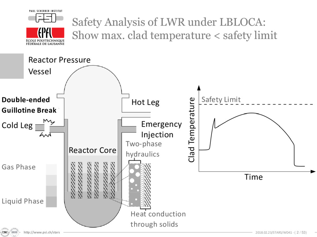
LWR under LBLOCA: Show max. clad temperature < safety limit Cold Leg Hot Leg Gas Phase Liquid Phase Double-ended Guillotine Break Emergency Injection Two-phase hydraulics Heat conduction through solids Reactor Core Reactor Pressure Vessel Clad Temperature Time Safety Limit
in Physical Model Parameters FLECHT-SEASET Westinghouse, USA Excerpt from the TRACE Code Theory Manual: • “…the approximate value of the coefficient in Eq. (4-119) was determined from data comparisons with FLECHT-SEASET high flooding rate reflood data…” (pp. 164) • “In TRACE, the above interfacial drag coefficient has been reduced by a factor of ¾ to better match FLECHT-SEASET high flooding rate reflood data, so…” (pp. 166) No statement of uncertainty on these parameters
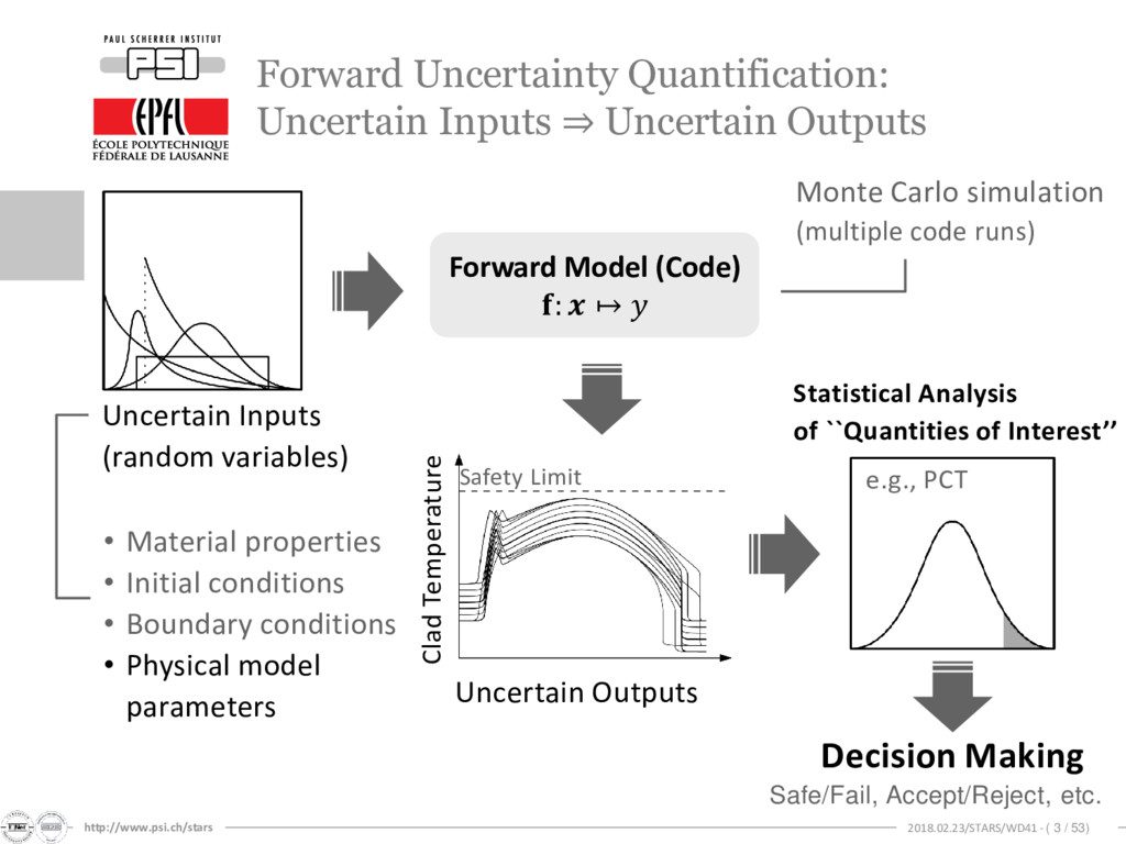
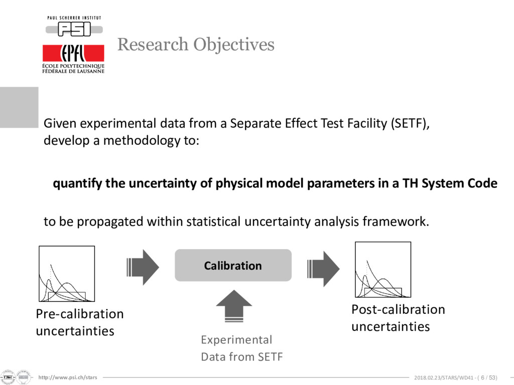
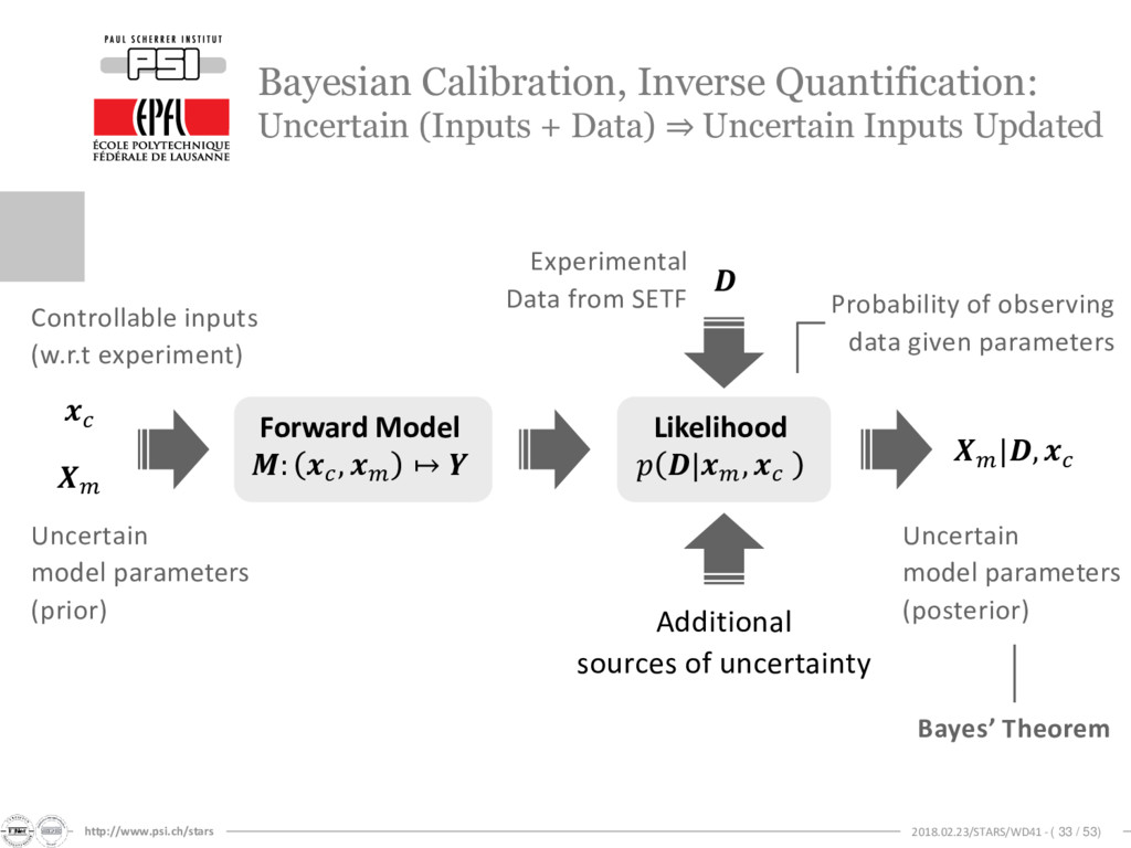
experimental data from a Separate Effect Test Facility (SETF), develop a methodology to: quantify the uncertainty of physical model parameters in a TH System Code to be propagated within statistical uncertainty analysis framework. Calibration Pre-calibration uncertainties Post-calibration uncertainties Experimental Data from SETF
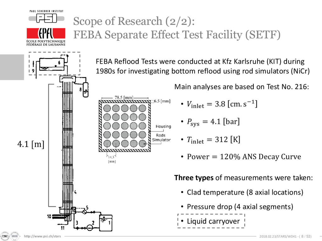
(2/2): FEBA Separate Effect Test Facility (SETF) FEBA Reflood Tests were conducted at Kfz Karlsruhe (KIT) during 1980s for investigating bottom reflood using rod simulators (NiCr) 4.1 [m] Three types of measurements were taken: • Clad temperature (8 axial locations) • Pressure drop (4 axial segments) • Liquid carryover Main analyses are based on Test No. 216: • inlet = 3.8 cm. s−1 • sys = 4.1 bar • inlet = 312 K • Power = 120% ANS Decay Curve
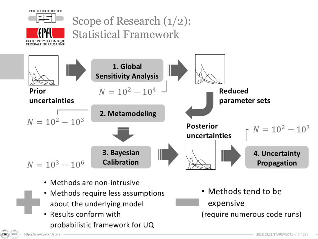
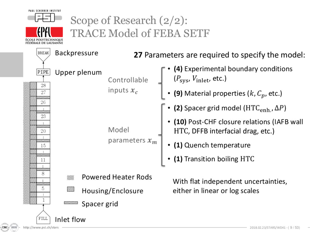
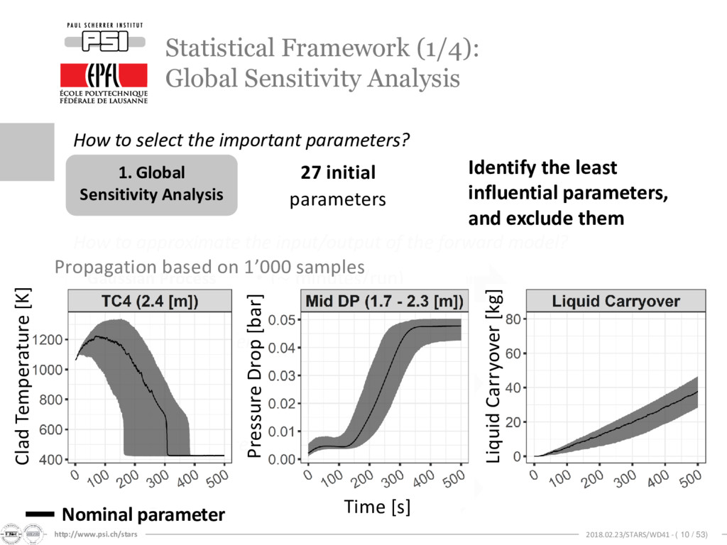
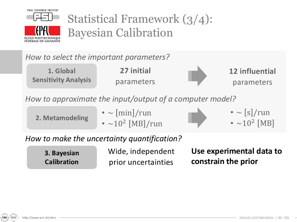
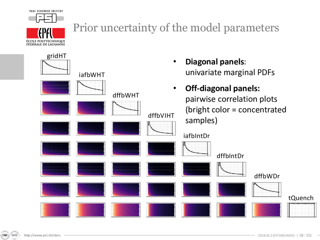
Global Sensitivity Analysis 1. Global Sensitivity Analysis Gaussian Process Metamodeling Bayesian Calibration Uncertainty Propagation How to approximate the input/output of the forward model? How to make the inference (quantification)? Is the quantified uncertainty useful? 27 initial parameters • (~ minutes/run) • (~102 MBytes/run) How to select the important parameters? Clad Temperature [K] Pressure Drop [bar] Time [s] Liquid Carryover [kg] Propagation based on 1’000 samples Identify the least influential parameters, and exclude them Nominal parameter
Δ ≡ ቤ ≅ 1, , … , , + Δ , ⋯ , , − ( ) Δ Base point Questions on robustness: • Weigh heavily on the region around a single base point • Assumption on linearity across input parameter space Perturbed points
The Morris Screening and Sobol’ Total-Effect Elementary effect : Perturbation of one parameter at a time ≡ + Δ ⋅ − () Δ Grid size ≡ ~ ~ Sobol’ total-effect index for : Expectation Variance
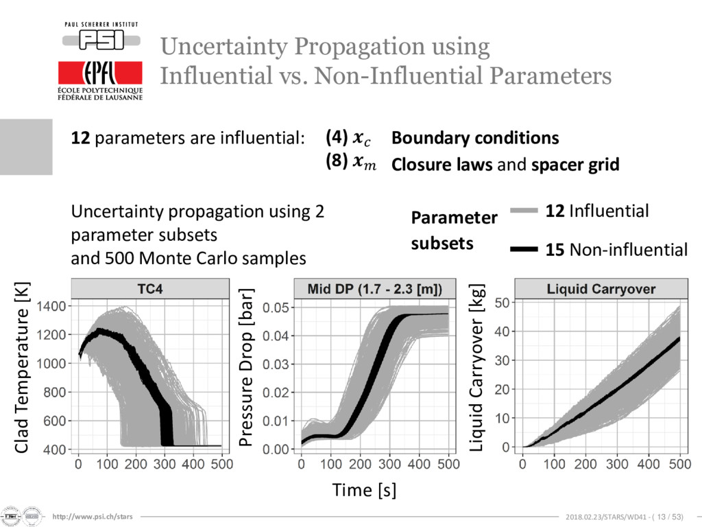
Influential vs. Non-Influential Parameters Clad Temperature [K] Pressure Drop [bar] Time [s] Liquid Carryover [kg] 12 Influential 15 Non-influential Parameter subsets Uncertainty propagation using 2 parameter subsets and 500 Monte Carlo samples 12 parameters are influential: (4) (8) Boundary conditions Closure laws and spacer grid
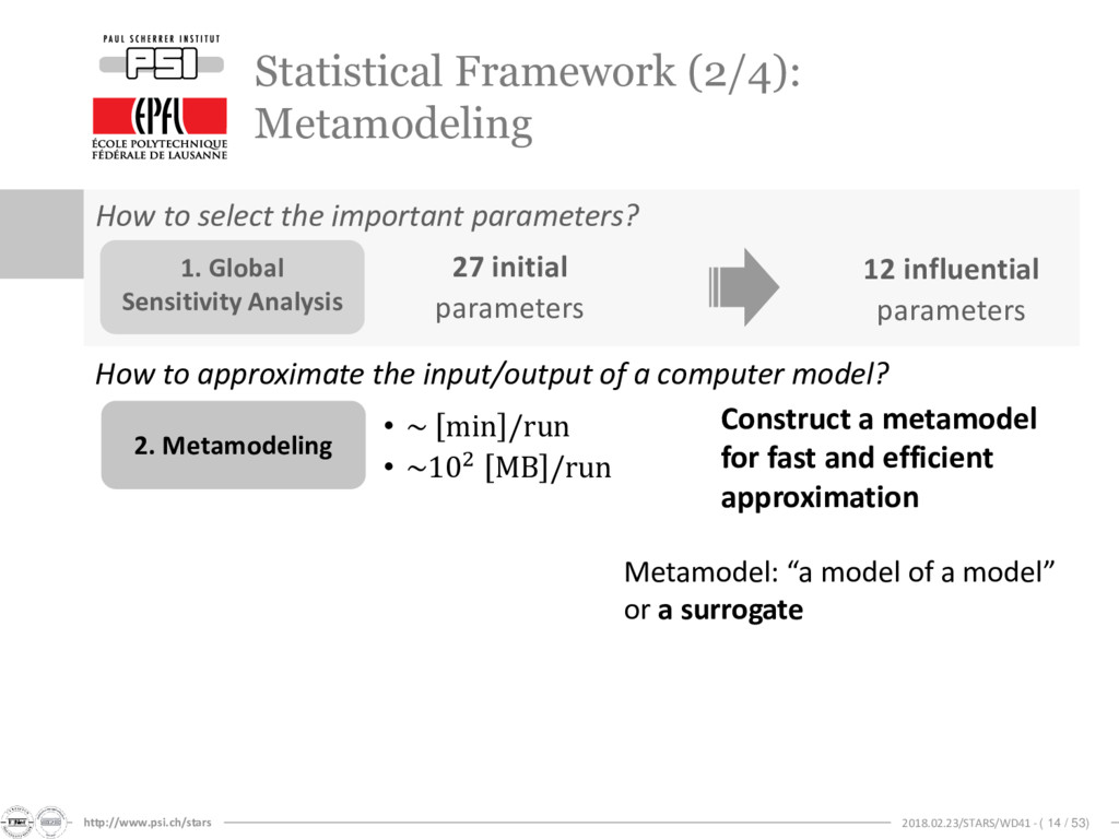
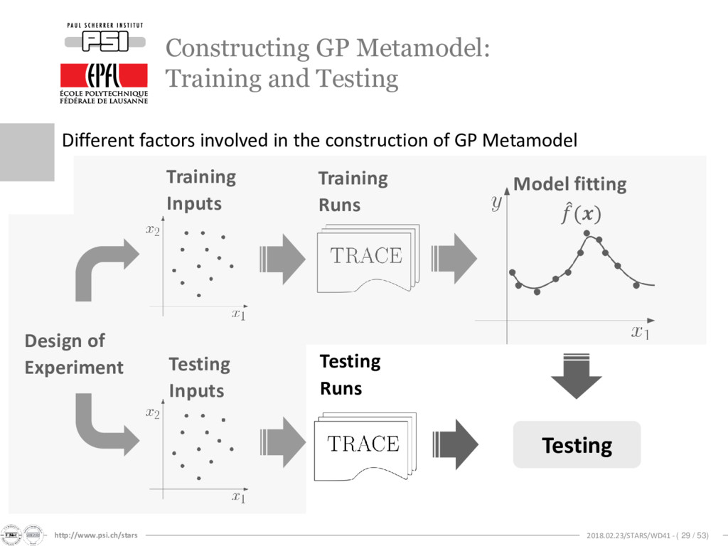
Metamodeling 1. Global Sensitivity Analysis 2. Metamodeling How to select the important parameters? How to approximate the input/output of a computer model? 27 initial parameters 12 influential parameters • ~ min /run • ~102 MB /run Construct a metamodel for fast and efficient approximation Metamodel: “a model of a model” or a surrogate
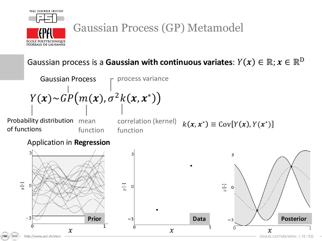
Gaussian Process (GP) Metamodel , ∗ ≡ Cov , (∗) ()~ (), 2 , ∗ Probability distribution of functions mean function process variance correlation (kernel) function Gaussian Process Gaussian process is a Gaussian with continuous variates: ∈ ℝ; ∈ ℝD Application in Regression
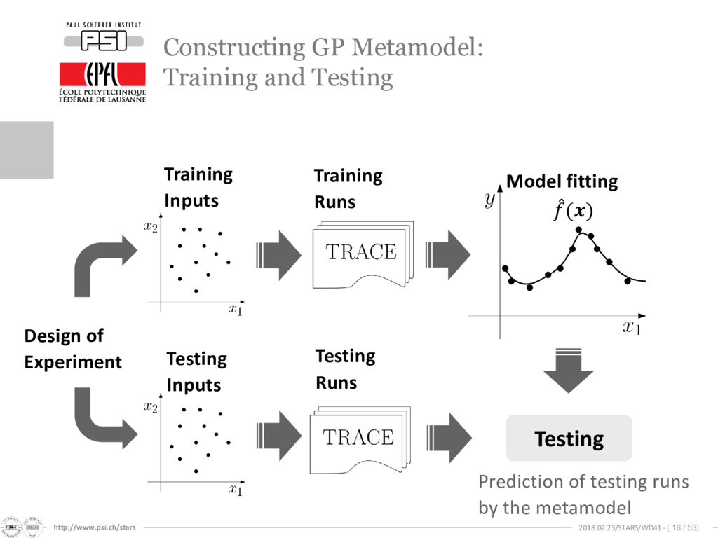
Training and Testing Testing Design of Experiment Training Runs Testing Runs መ () Model fitting Training Inputs Testing Inputs Prediction of testing runs by the metamodel
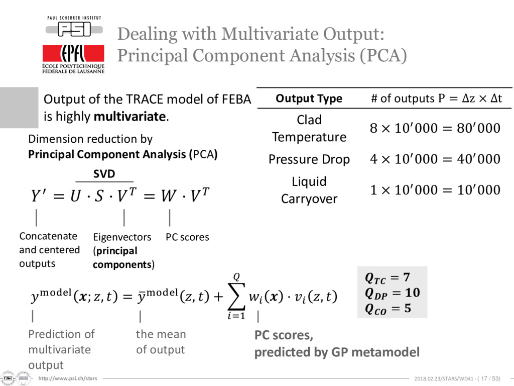
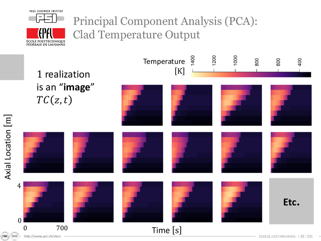
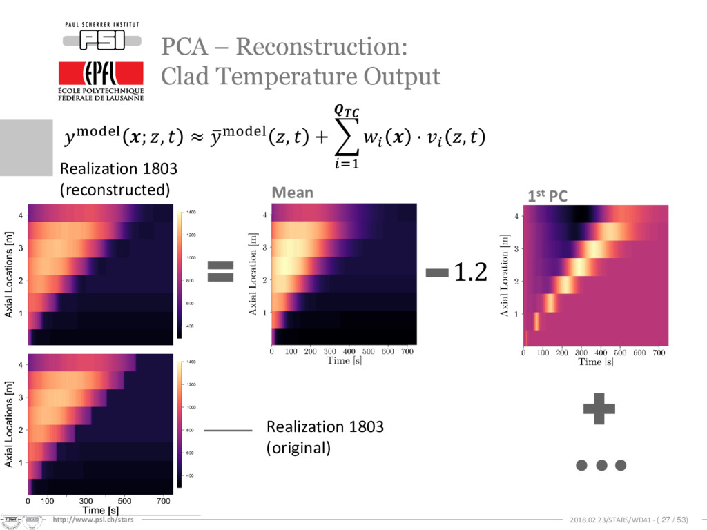
Output: Principal Component Analysis (PCA) Output of the TRACE model of FEBA is highly multivariate. Output Type # of outputs P = Δz × Δt Clad Temperature 8 × 10′000 = 80′000 Pressure Drop 4 × 10′000 = 40′000 Liquid Carryover 1 × 10′000 = 10′000 Dimension reduction by Principal Component Analysis (PCA) ′ = ⋅ ⋅ = ⋅ SVD Concatenate and centered outputs Eigenvectors (principal components) PC scores model ; , = ത model , + =1 ⋅ , PC scores, predicted by GP metamodel the mean of output Prediction of multivariate output = = =
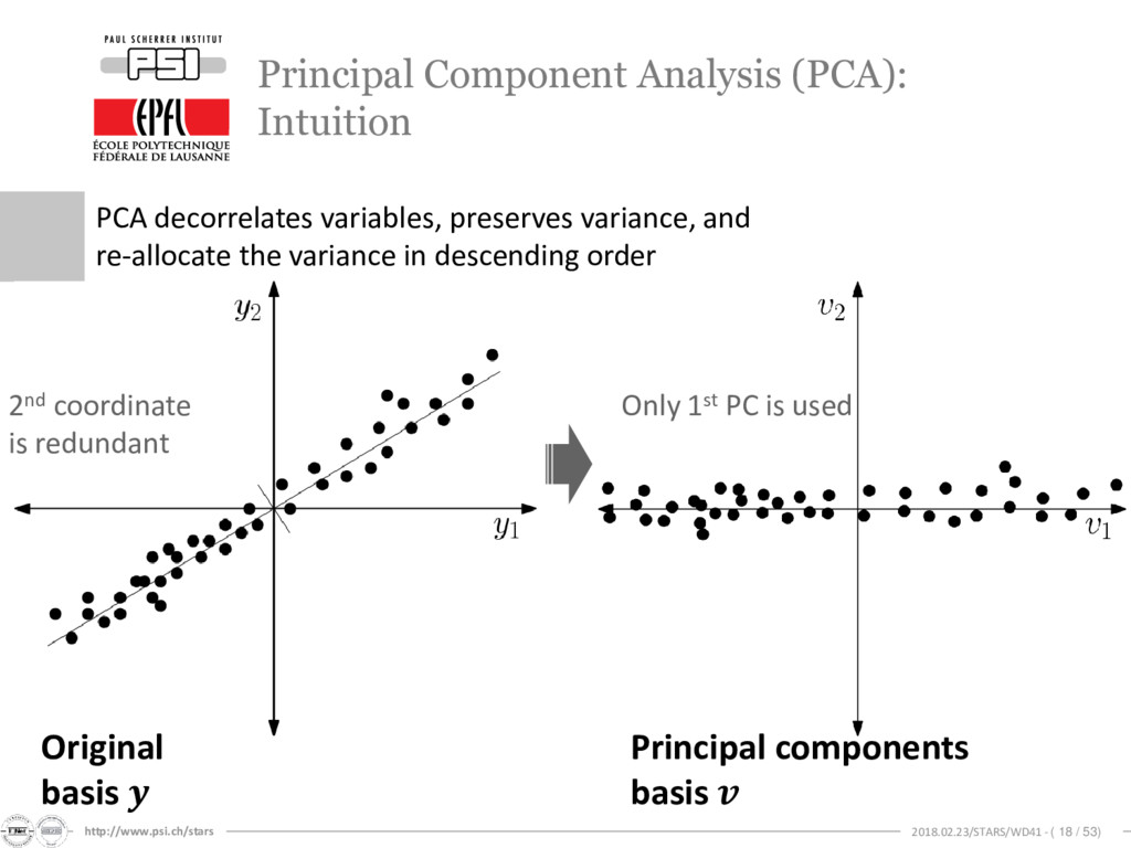
(PCA): Intuition PCA decorrelates variables, preserves variance, and re-allocate the variance in descending order Original basis Principal components basis 2nd coordinate is redundant Only 1st PC is used
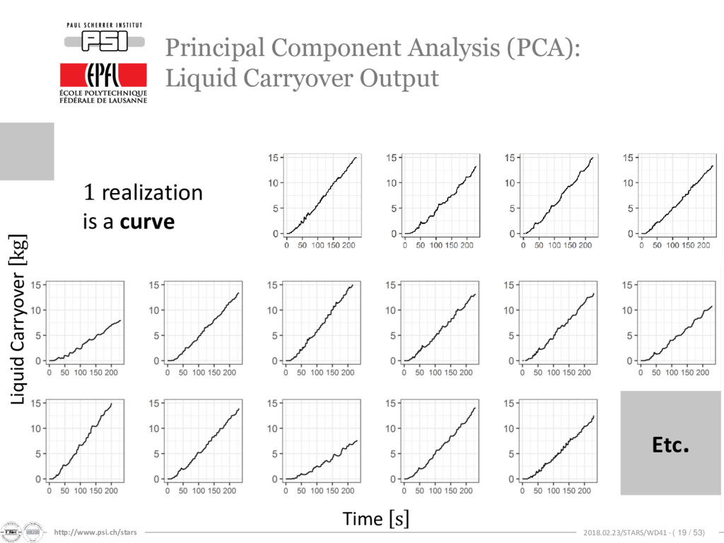
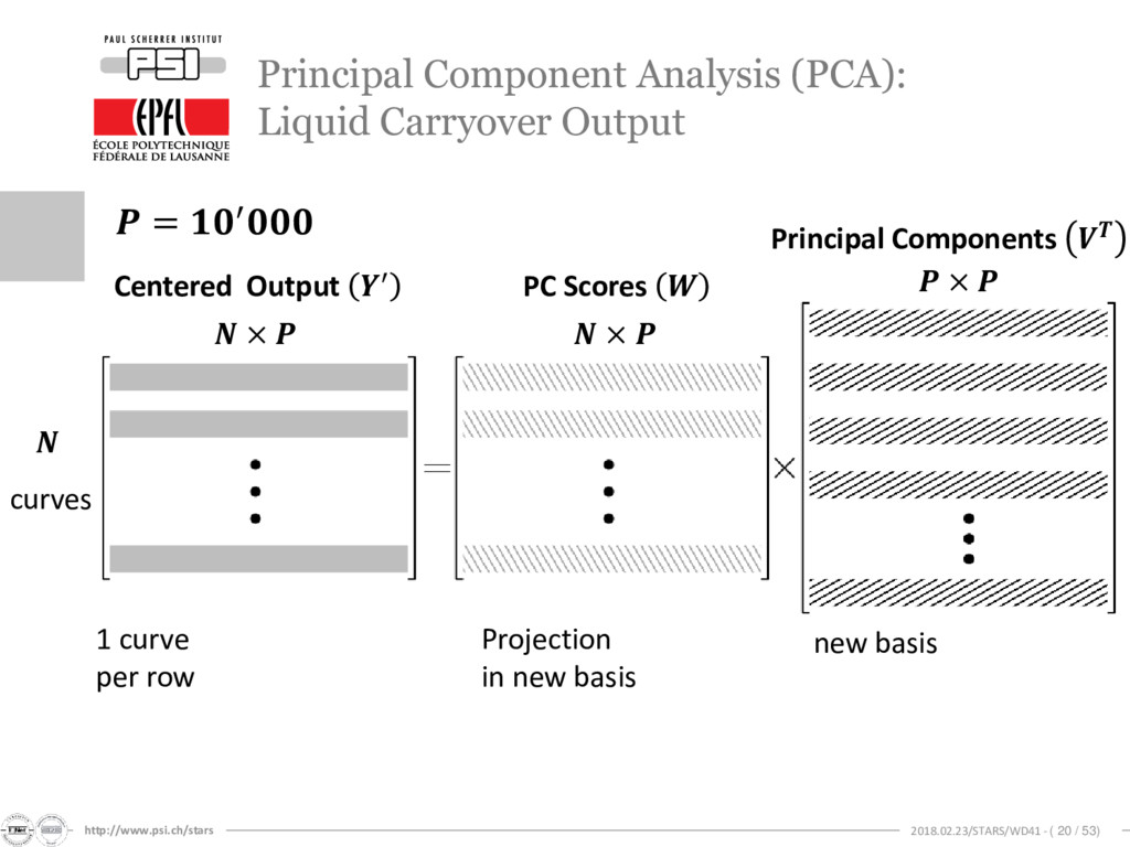
Analysis (PCA): Liquid Carryover Output Centered Output ′ PC Scores Principal Components × × curves = ′ 1 curve per row Projection in new basis new basis
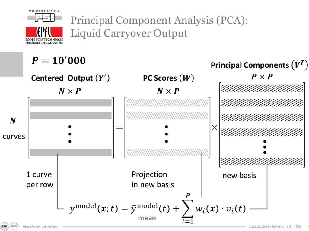
= ത model + =1 ⋅ Principal Component Analysis (PCA): Liquid Carryover Output Centered Output ′ PC Scores Principal Components × × curves = ′ mean 1 curve per row Projection in new basis new basis
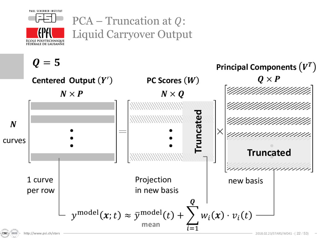
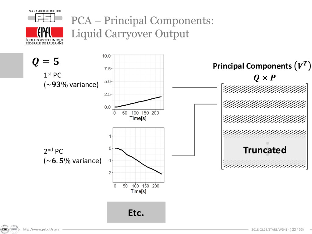
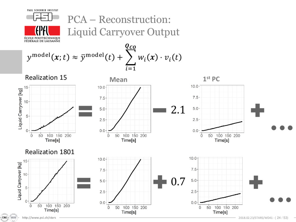
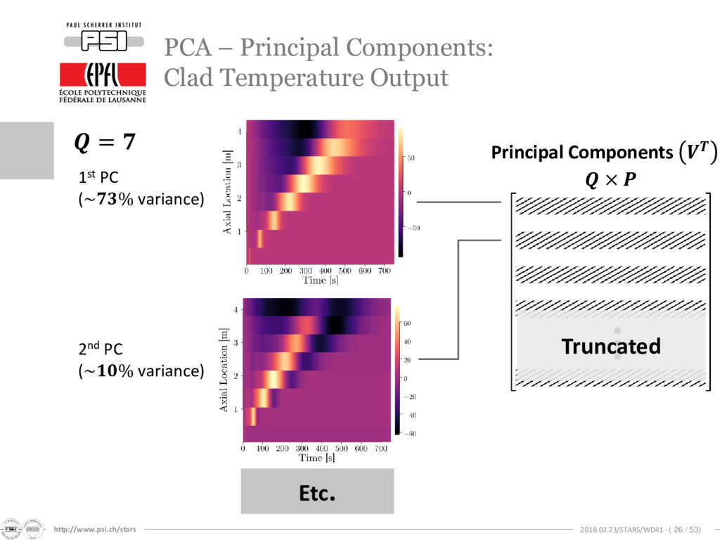
; ≈ ത model + =1 ⋅ PCA – Truncation at : Liquid Carryover Output × × curves Truncated = mean 1 curve per row Projection in new basis new basis Centered Output ′ PC Scores Principal Components
GP Metamodel: Summary Centered Output ′ PC Scores Principal Components × × runs PC is used to construct any new realizations Metamodel is used to predict model ; , = ത model , + =1 ⋅ , 1 curve per row Truncated Truncated
Training and Testing Testing Design of Experiment Training Runs Testing Runs መ () Model fitting Different factors involved in the construction of GP Metamodel Training Inputs Testing Inputs
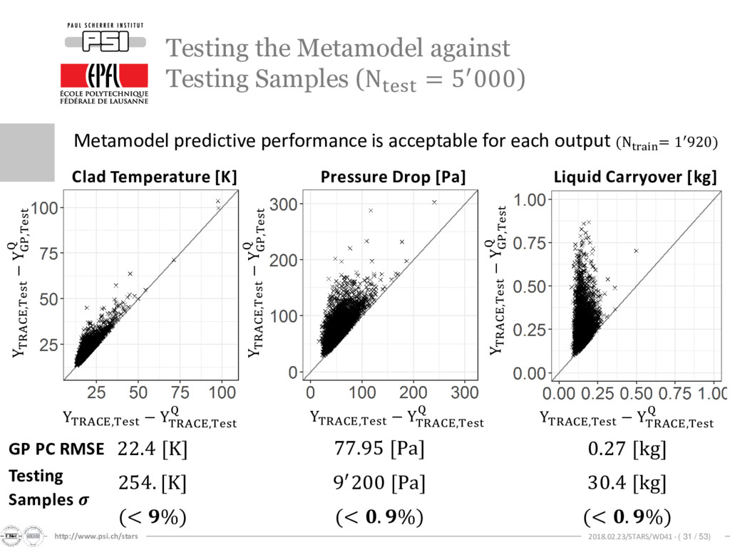
against Testing Samples Metamodel predictive performance is assessed by comparison against large independent test data (i.e. actual TRACE runs) YTRACE,Test − Y TRACE,Test Q YTRACE,Test − Y GP,Test Q • Dimension reduction error • Due to smaller to reconstruct the full output space X-axis: Y-axis: • Dimension reduction error and GP error • Due to (also) miss-prediction of PC scores Both are in terms of RMSE YTRACE,Test − Y TRACE,Test Q YTRACE,Test − Y GP,Test Q
Bayesian Calibration 1. Global Sensitivity Analysis 2. Metamodeling 3. Bayesian Calibration How to select the important parameters? How to approximate the input/output of a computer model? How to make the uncertainty quantification? 27 initial parameters 12 influential parameters • ~ min /run • ~102 MB /run Wide, independent prior uncertainties • ~ s /run • ~102 MB Use experimental data to constrain the prior
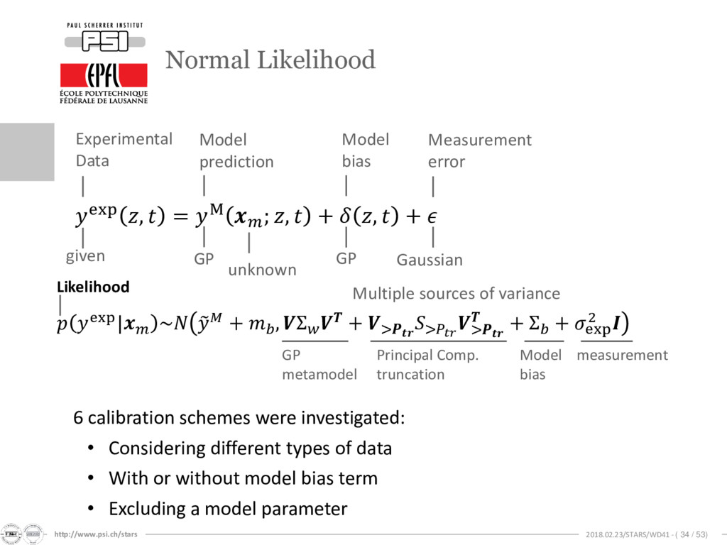
~ + , Σ + > > > + Σ + exp 2 GP metamodel Principal Comp. truncation Model bias measurement Multiple sources of variance Likelihood exp , = M ; , + , + Model prediction Model bias Measurement error Experimental Data 6 calibration schemes were investigated: • Considering different types of data • With or without model bias term • Excluding a model parameter GP GP Gaussian given unknown
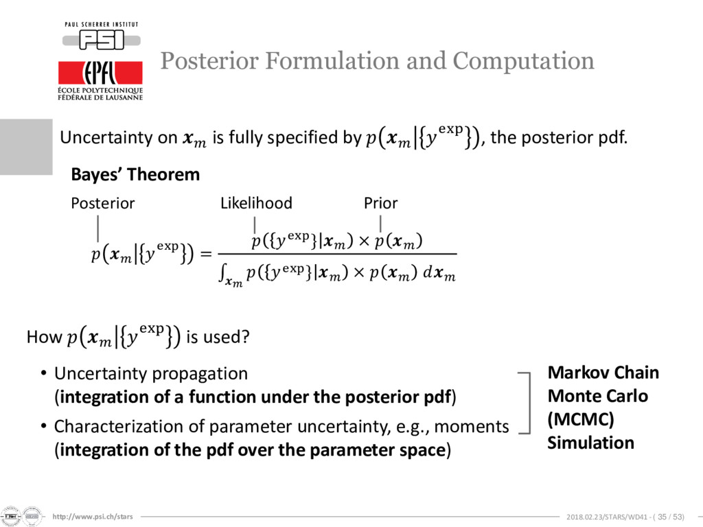
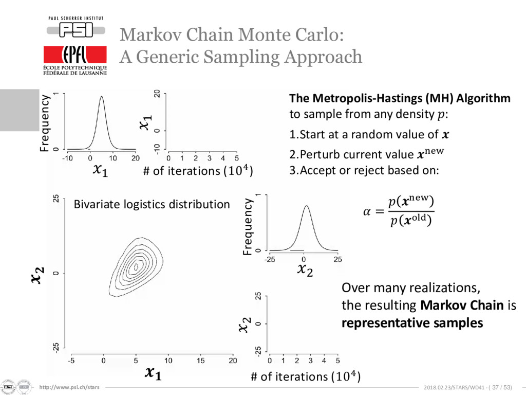
Computation Bayes’ Theorem exp = exp} × exp} × Posterior Likelihood Prior Uncertainty on is fully specified by exp , the posterior pdf. Markov Chain Monte Carlo (MCMC) Simulation How exp is used? • Uncertainty propagation (integration of a function under the posterior pdf) • Characterization of parameter uncertainty, e.g., moments (integration of the pdf over the parameter space)
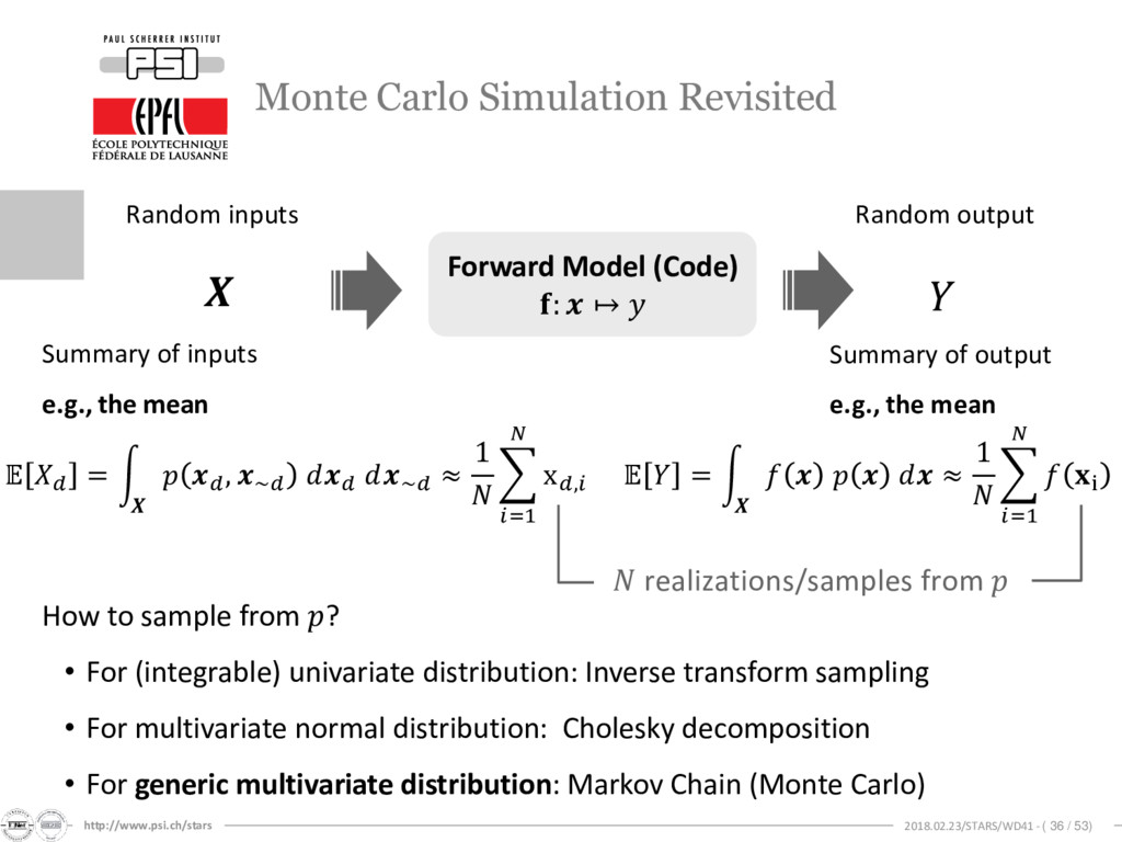
~ ~ ≈ 1 =1 x, Monte Carlo Simulation Revisited = න ≈ 1 =1 i Forward Model (Code) : ↦ Summary of output e.g., the mean Random inputs Random output Summary of inputs e.g., the mean How to sample from ? • For (integrable) univariate distribution: Inverse transform sampling • For multivariate normal distribution: Cholesky decomposition • For generic multivariate distribution: Markov Chain (Monte Carlo) realizations/samples from
Carlo: A Generic Sampling Approach 1 1 # of iterations (104) # of iterations (104) 2 Frequency 2 Frequency The Metropolis-Hastings (MH) Algorithm to sample from any density : 1.Start at a random value of 2.Perturb current value new 3.Accept or reject based on: = new old Over many realizations, the resulting Markov Chain is representative samples Bivariate logistics distribution
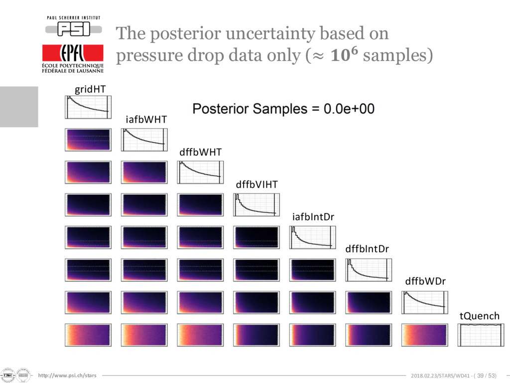
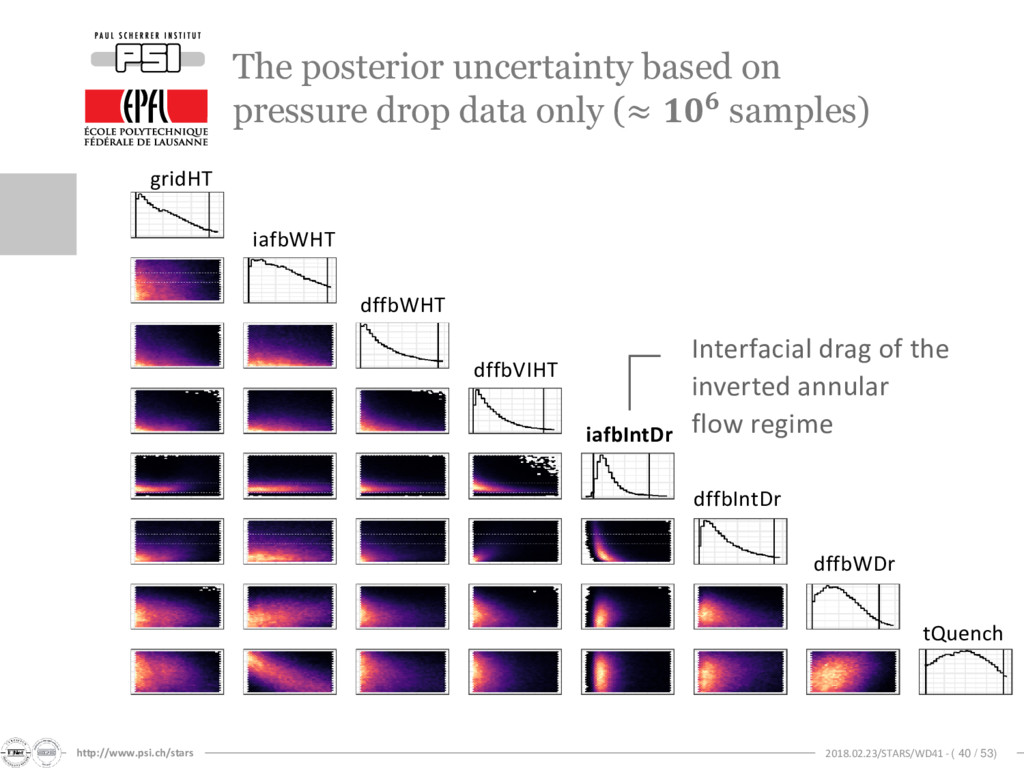
based on pressure drop data only (≈ samples) gridHT iafbWHT dffbWHT dffbVIHT iafbIntDr dffbIntDr dffbWDr tQuench Interfacial drag of the inverted annular flow regime
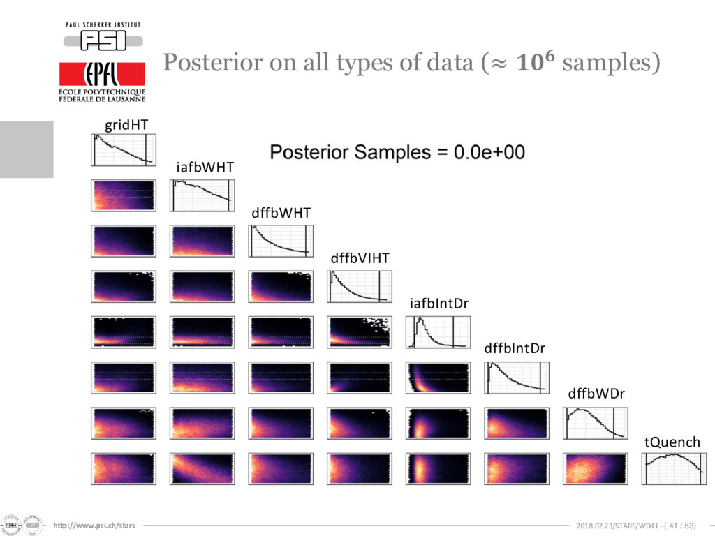
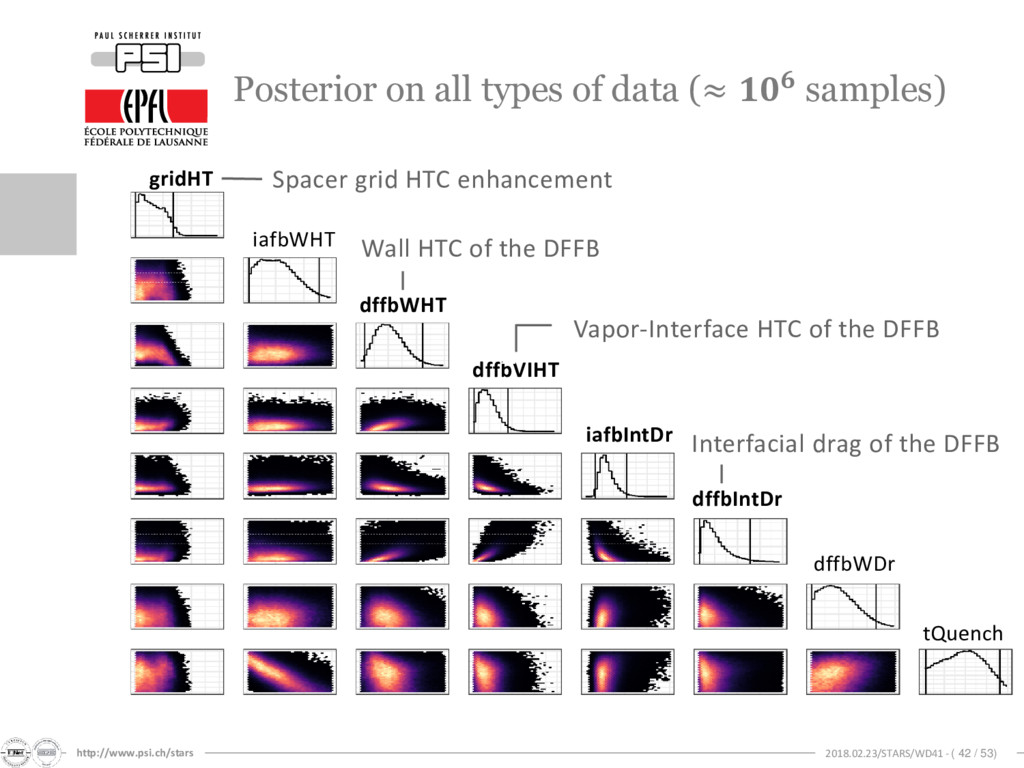
types of data (≈ samples) gridHT iafbWHT dffbWHT dffbVIHT iafbIntDr dffbIntDr dffbWDr tQuench Vapor-Interface HTC of the DFFB Spacer grid HTC enhancement Interfacial drag of the DFFB Wall HTC of the DFFB
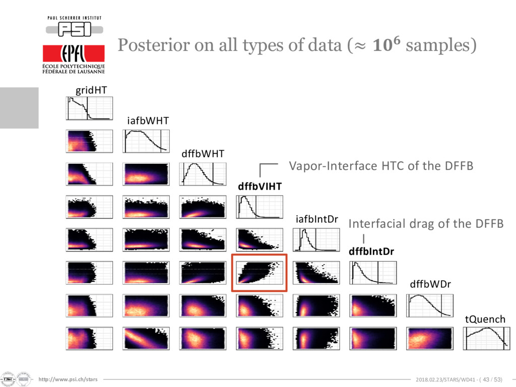
types of data (≈ samples) gridHT iafbWHT dffbWHT dffbVIHT iafbIntDr dffbIntDr dffbWDr tQuench Vapor-Interface HTC of the DFFB Interfacial drag of the DFFB
Samples are Correlated (i.e., a set of “collectively-fitted” values) Clad Temperature [K] Middle assembly Top assembly Uncertainty propagation on FEBA Test. No. 216 (the calibration data) based on 1’000 Monte Carlo samples. Prior Posterior, Correlated Posterior, Independent Exp. Data
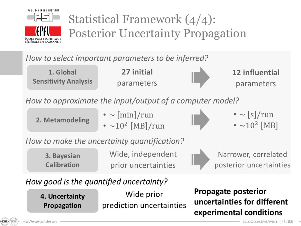
Posterior Uncertainty Propagation 1. Global Sensitivity Analysis 2. Metamodeling 3. Bayesian Calibration How to select important parameters to be inferred? How to approximate the input/output of a computer model? How to make the uncertainty quantification? How good is the quantified uncertainty? 27 initial parameters 12 influential parameters • ~ min /run • ~102 MB /run Wide, independent prior uncertainties • ~ s /run • ~102 MB Narrower, correlated posterior uncertainties 4. Uncertainty Propagation Wide prior prediction uncertainties Propagate posterior uncertainties for different experimental conditions
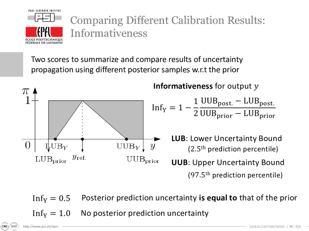
Results: Informativeness Two scores to summarize and compare results of uncertainty propagation using different posterior samples w.r.t the prior InfY = 1 − 1 2 UUBpost. − LUBpost. UUBprior − LUBprior LUB: Lower Uncertainty Bound (2.5th prediction percentile) (97.5th prediction percentile) UUB: Upper Uncertainty Bound Informativeness for output InfY = 0.5 InfY = 1.0 Posterior prediction uncertainty is equal to that of the prior No posterior prediction uncertainty
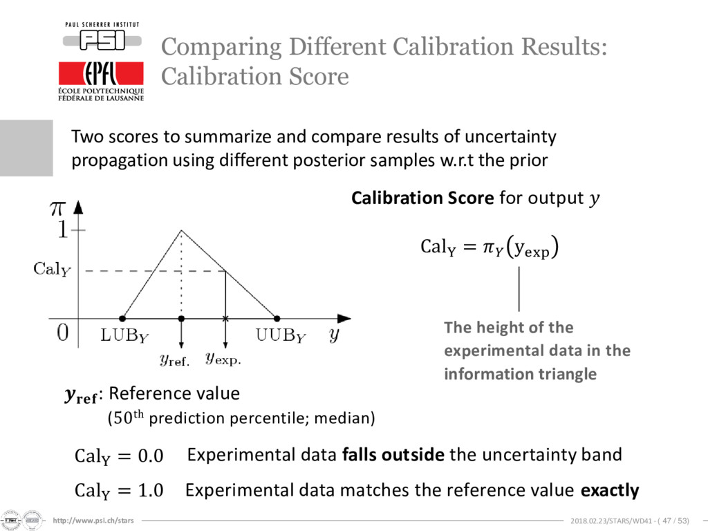
Results: Calibration Score Two scores to summarize and compare results of uncertainty propagation using different posterior samples w.r.t the prior Calibration Score for output CalY = 0.0 CalY = 1.0 Experimental data falls outside the uncertainty band Experimental data matches the reference value exactly CalY = yexp The height of the experimental data in the information triangle : Reference value (50th prediction percentile; median)
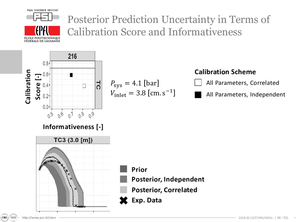
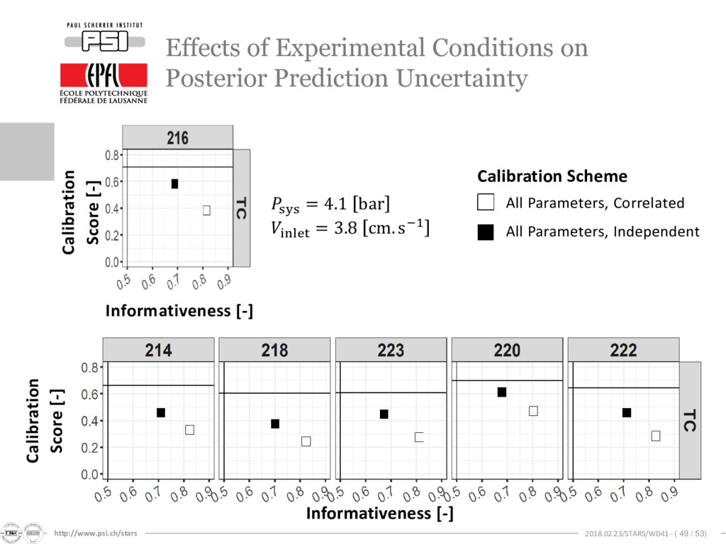
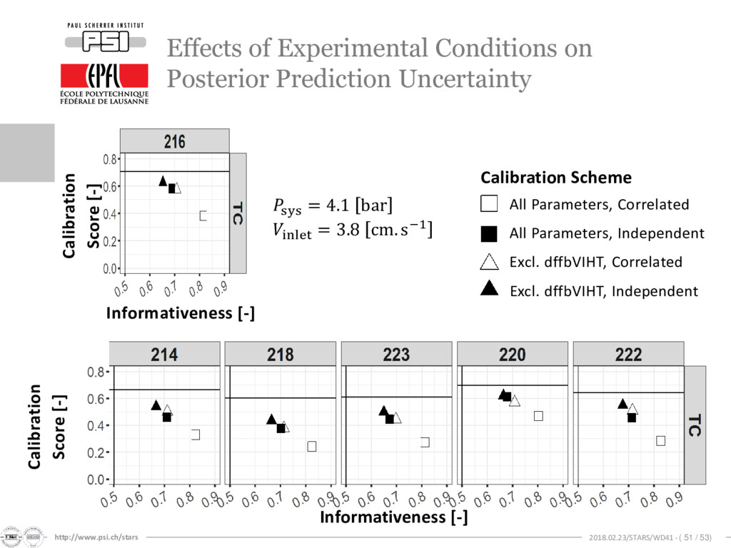
in Terms of Calibration Score and Informativeness Informativeness [-] sys = 4.1 bar inlet = 3.8 cm. s−1 Calibration Scheme All Parameters, Correlated All Parameters, Independent Calibration Score [-] Prior Posterior, Correlated Posterior, Independent Exp. Data
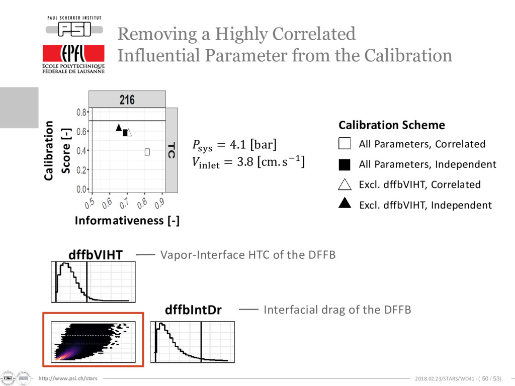
Correlated Influential Parameter from the Calibration sys = 4.1 bar inlet = 3.8 cm. s−1 Calibration Scheme All Parameters, Independent All Parameters, Correlated Excl. dffbVIHT, Independent Excl. dffbVIHT, Correlated Calibration Score [-] Informativeness [-] dffbVIHT dffbIntDr Vapor-Interface HTC of the DFFB Interfacial drag of the DFFB
and application of tools based on statistical framework for quantifying the physical model parameters in the TRACE code Motivation: Objectives: Contribution: Given data from a separate effect test facility, develop a methodology to systematically quantify the uncertainty of the parameters in the TRACE code Uncertainty in physical model parameters are often derived mainly based on expert-judgment and on a particular experimental data
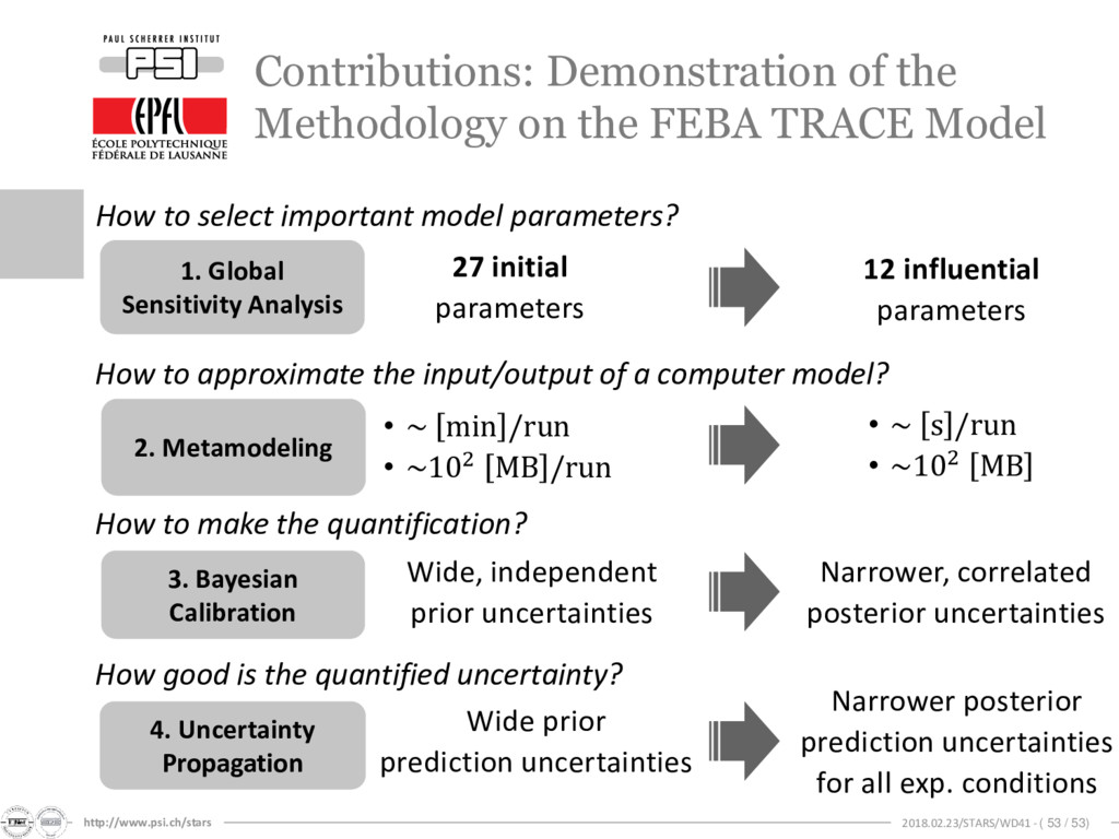
the Methodology on the FEBA TRACE Model 1. Global Sensitivity Analysis 2. Metamodeling 3. Bayesian Calibration How to select important model parameters? How to approximate the input/output of a computer model? How to make the quantification? 27 initial parameters 12 influential parameters • ~ min /run • ~102 MB /run Wide, independent prior uncertainties • ~ s /run • ~102 MB Narrower, correlated posterior uncertainties 4. Uncertainty Propagation Narrower posterior prediction uncertainties for all exp. conditions Wide prior prediction uncertainties How good is the quantified uncertainty?
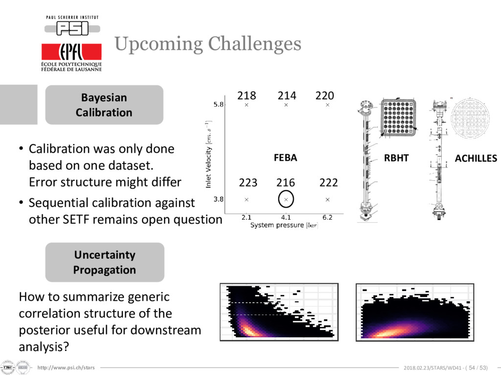
Calibration Uncertainty Propagation 216 214 How to summarize generic correlation structure of the posterior useful for downstream analysis? • Calibration was only done based on one dataset. Error structure might differ • Sequential calibration against other SETF remains open question ACHILLES RBHT 220 222 223 218 FEBA
your attention. My sincere gratitude to: • Prof. A. Pautz • Mr. O. Zerkak • Dr. G. Perret • Mr. Ph. Jacquemoud • Dr. M. Hursin • Dr. D. Rochman • Dr. I. Clifford • Mr. H. Ferroukhi • Other members of STARS The jury members: • Dr. J. Baccou • Prof. R. Houdré • Prof. B. Sudret • Dr. W. Zwermann Additional acknowledgments: •Swiss Federal Nuclear Safety Inspectorate (ENSI) •Swiss Federal Office of Energy (BFE) 1.“Global Sensitivity Analysis of Transient Code Output applied to a Reflood Experiment Model using TRACE Code,” NSE, vol. 184, no. 6, 2016. 2.“Bayesian Calibration of Thermal-Hydraulics Model with Time-Dependent Output,” NUTHOS-11, 2016. 3.“A Methodology for Global Sensitivity Analysis of Transient Code Output applied to Reflood Experiment Model using TRACE,” NURETH-16, 2015. 4.“Sensitivity Analysis of Bottom Reflood Simulation using the Morris Screening Method,” NUTHOS-10, 2014. 5.“Exploring Variability in Reflood Simulation Results: an Application of Functional Data Analysis,” NUTHOS-10, 2014.
![http://www.psi.ch/stars 2018.02.23/STARS/WD41 - ( 44 / 53) Time [s] Posterior](https://files.speakerdeck.com/presentations/16652f93ed3a4df2865d634a8f2cd201/slide_43.jpg)