Probability and statistical testing

Transcript

1. Probability and statistical testing Deependra Dhakal Academic year 2019-2020 Gokuleshwor Agriculture and Animal Science College Tribhuwan University ddhakal.rookie@gmail.com https://rookie.rbind.io
2. The probability rules 2
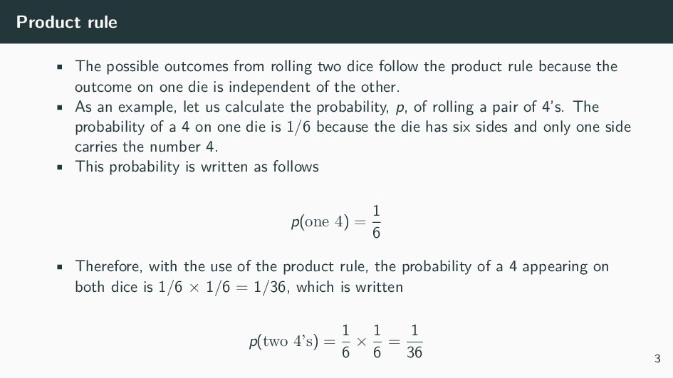
3. Product rule • The possible outcomes from rolling two dice follow the product rule because the outcome on one die is independent of the other. • As an example, let us calculate the probability, p, of rolling a pair of 4’s. The probability of a 4 on one die is 1/6 because the die has six sides and only one side carries the number 4. • This probability is written as follows p(one 4) = 1 6 • Therefore, with the use of the product rule, the probability of a 4 appearing on both dice is 1/6 × 1/6 = 1/36, which is written p(two 4’s) = 1 6 × 1 6 = 1 36 3
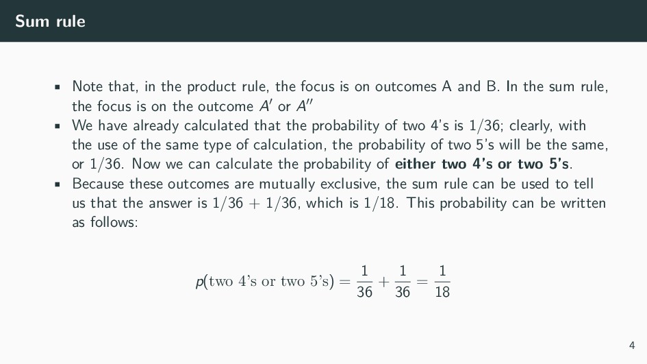
4. Sum rule • Note that, in the product rule, the focus is on outcomes A and B. In the sum rule, the focus is on the outcome A′ or A′′ • We have already calculated that the probability of two 4’s is 1/36; clearly, with the use of the same type of calculation, the probability of two 5’s will be the same, or 1/36. Now we can calculate the probability of either two 4’s or two 5’s. • Because these outcomes are mutually exclusive, the sum rule can be used to tell us that the answer is 1/36 + 1/36, which is 1/18. This probability can be written as follows: p(two 4’s or two 5’s) = 1 36 + 1 36 = 1 18 4
5. Problem: Probability rules • What proportion of the progenies will be suitable to be used as tester parent in the cross between two parental genotypes: A/a; b/b; C/c; D/d; E/e × a/a; b/b; c/c; d/d; E/e • Approach using product rule. 5
6. How many progenies do we need ? • Assume we need to estimate how many progeny plants need to be grown to stand a reasonable chance of obtaining the desired genotype a/a; b/b; c/c; d/d; e/e. • First calculate the proportion of progeny that is expected to be of that genotype, as such we need at least 256 progeny to stand an average chance of obtaining one individual plant of the desired genotype. • The probability of obtaining one “success” (a fully recessive plant) out of 256 has to be considered more carefully. This is the average probability of success. Unfortunately, if we isolated and tested 256 progeny, we would very likely have no success at all, simply from bad luck. • A more meaningful question to as ask would, hence be, what sample size do we need to be 95% confident that we will obtain at least one success ? • Probability of obtaining at least one success can be expressed as: 1 − ( 255 256 )n 6
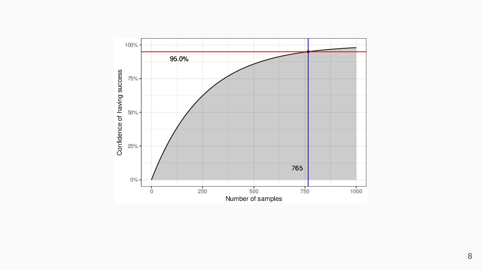
7. • To be 95% confident that our sample will contain at least one genotype we intended, we solve: 1 − ( 255 256 )n = 0.95 • Solving for n gives 765, which is the right amount of progeny samples to be raised to assure 95% success of having 1 individual out of 256 totals. 7
8. 95.0% 95.0% 765 765 0% 25% 50% 75% 100% 0 250 500 750 1000 Number of samples Confidence of having success 8
9. Using χ2 test on monohybrid and dihybrid ratios 9
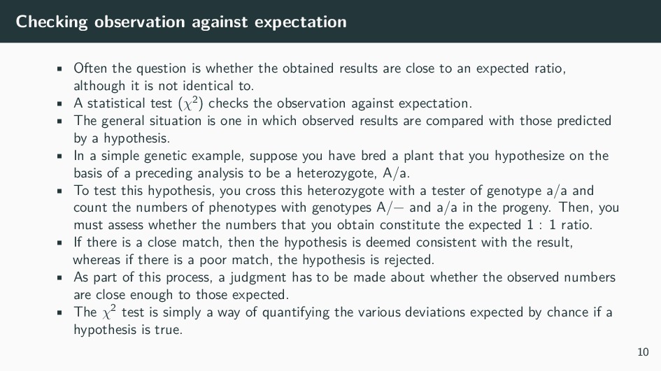
10. Checking observation against expectation • Often the question is whether the obtained results are close to an expected ratio, although it is not identical to. • A statistical test (χ2) checks the observation against expectation. • The general situation is one in which observed results are compared with those predicted by a hypothesis. • In a simple genetic example, suppose you have bred a plant that you hypothesize on the basis of a preceding analysis to be a heterozygote, A/a. • To test this hypothesis, you cross this heterozygote with a tester of genotype a/a and count the numbers of phenotypes with genotypes A/− and a/a in the progeny. Then, you must assess whether the numbers that you obtain constitute the expected 1 : 1 ratio. • If there is a close match, then the hypothesis is deemed consistent with the result, whereas if there is a poor match, the hypothesis is rejected. • As part of this process, a judgment has to be made about whether the observed numbers are close enough to those expected. • The χ2 test is simply a way of quantifying the various deviations expected by chance if a hypothesis is true. 10
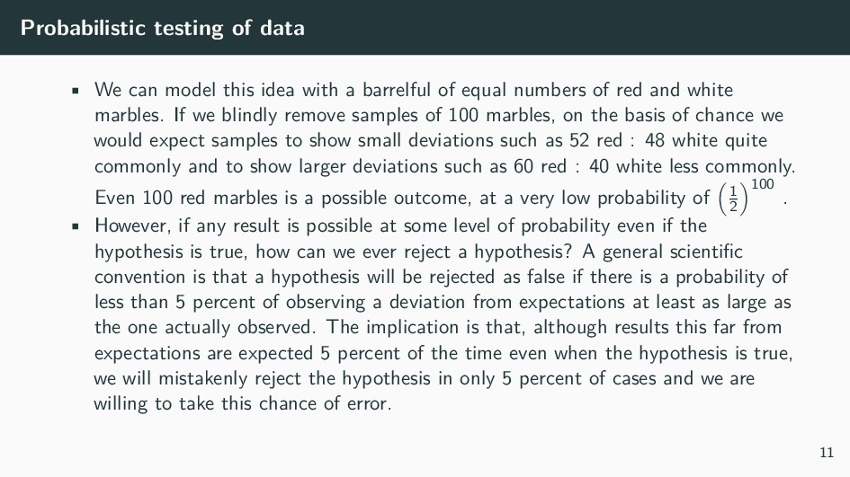
11. Probabilistic testing of data • We can model this idea with a barrelful of equal numbers of red and white marbles. If we blindly remove samples of 100 marbles, on the basis of chance we would expect samples to show small deviations such as 52 red : 48 white quite commonly and to show larger deviations such as 60 red : 40 white less commonly. Even 100 red marbles is a possible outcome, at a very low probability of ( 1 2 )100 . • However, if any result is possible at some level of probability even if the hypothesis is true, how can we ever reject a hypothesis? A general scientific convention is that a hypothesis will be rejected as false if there is a probability of less than 5 percent of observing a deviation from expectations at least as large as the one actually observed. The implication is that, although results this far from expectations are expected 5 percent of the time even when the hypothesis is true, we will mistakenly reject the hypothesis in only 5 percent of cases and we are willing to take this chance of error. 11
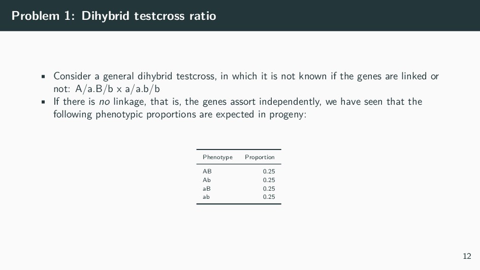
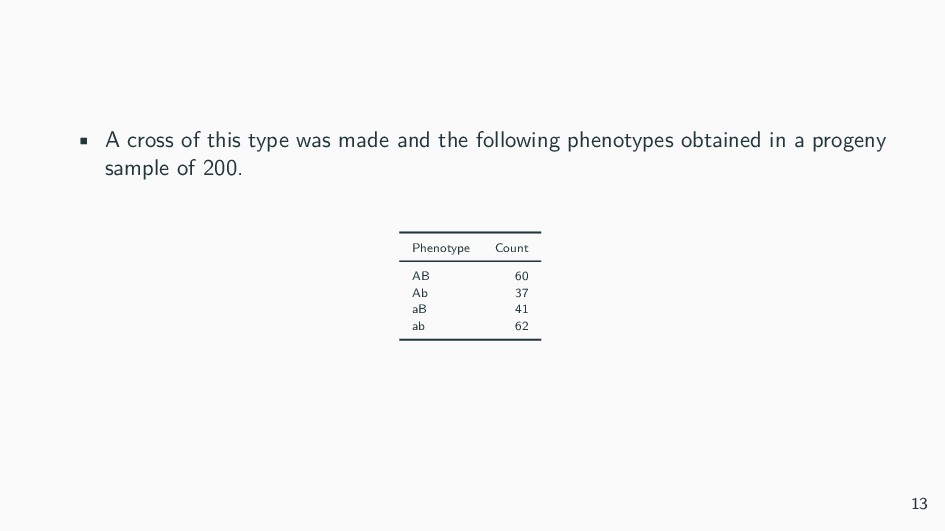
12. Problem 1: Dihybrid testcross ratio • Consider a general dihybrid testcross, in which it is not known if the genes are linked or not: A/a.B/b x a/a.b/b • If there is no linkage, that is, the genes assort independently, we have seen that the following phenotypic proportions are expected in progeny: Phenotype Proportion AB 0.25 Ab 0.25 aB 0.25 ab 0.25 12
13. • A cross of this type was made and the following phenotypes obtained in a progeny sample of 200. Phenotype Count AB 60 Ab 37 aB 41 ab 62 13
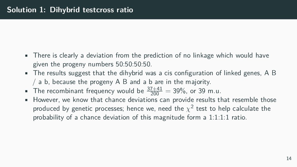
14. Solution 1: Dihybrid testcross ratio • There is clearly a deviation from the prediction of no linkage which would have given the progeny numbers 50:50:50:50. • The results suggest that the dihybrid was a cis configuration of linked genes, A B / a b, because the progeny A B and a b are in the majority. • The recombinant frequency would be 37+41 200 = 39%, or 39 m.u. • However, we know that chance deviations can provide results that resemble those produced by genetic processes; hence we, need the χ2 test to help calculate the probability of a chance deviation of this magnitude form a 1:1:1:1 ratio. 14
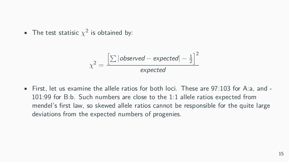
15. • The test statisic χ2 is obtained by: χ2 = [∑ |observed − expected| − 1 2 ]2 expected • First, let us examine the allele ratios for both loci. These are 97:103 for A:a, and - 101:99 for B:b. Such numbers are close to the 1:1 allele ratios expected from mendel’s first law, so skewed allele ratios cannot be responsible for the quite large deviations from the expected numbers of progenies. 15
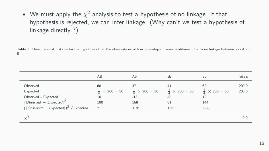
16. • We must apply the χ2 analysis to test a hypothesis of no linkage. If that hypothesis is rejected, we can infer linkage. (Why can’t we test a hypothesis of linkage directly ?) Table 1: Chi-square calculations for the hypothesis that the observations of four phenotypic classes is obtained due to no linkage between loci A and B. AB Ab aB ab Totals Observed 60 37 41 62 200.0 Expected 1 4 × 200 = 50 1 4 × 200 = 50 1 4 × 200 = 50 1 4 × 200 = 50 200.0 Observed - Expected 10 -13 -9 12 |Observed − Expected| 2 100 169 81 144 (|Observed − Expected|) 2 /Expected 2 3.38 1.62 2.88 χ 2 9.9 16
17. Table 2: The probabilities of exceeding different chi-square values for degrees of freedom from 1 to 50 when the expected hypothesis is true 0.005 0.01 0.025 0.05 0.1 0.9 0.95 0.975 0.99 0.995 1 7.9 6.6 5.0 3.8 2.7 0.02 0.00 0.00 0.00 0.00 2 10.6 9.2 7.4 6.0 4.6 0.21 0.10 0.05 0.02 0.01 3 12.8 11.3 9.3 7.8 6.2 0.58 0.35 0.22 0.11 0.07 4 14.9 13.3 11.1 9.5 7.8 1.06 0.71 0.48 0.30 0.21 5 16.8 15.1 12.8 11.1 9.2 1.61 1.15 0.83 0.55 0.41 6 18.6 16.8 14.4 12.6 10.6 2.20 1.64 1.24 0.87 0.68 7 20.3 18.5 16.0 14.1 12.0 2.83 2.17 1.69 1.24 0.99 8 21.9 20.1 17.5 15.5 13.4 3.49 2.73 2.18 1.65 1.34 9 23.6 21.7 19.0 16.9 14.7 4.17 3.33 2.70 2.09 1.73 10 25.2 23.2 20.5 18.3 16.0 4.87 3.94 3.25 2.56 2.16 11 26.8 24.7 21.9 19.7 17.3 5.58 4.57 3.82 3.05 2.60 12 28.3 26.2 23.3 21.0 18.6 6.30 5.23 4.40 3.57 3.07 13 29.8 27.7 24.7 22.4 19.8 7.04 5.89 5.01 4.11 3.57 14 31.3 29.1 26.1 23.7 21.1 7.79 6.57 5.63 4.66 4.07 15 32.8 30.6 27.5 25.0 22.3 8.55 7.26 6.26 5.23 4.60 16 34.3 32.0 28.9 26.3 23.5 9.31 7.96 6.91 5.81 5.14 17 35.7 33.4 30.2 27.6 24.8 10.09 8.67 7.56 6.41 5.70 18 37.2 34.8 31.5 28.9 26.0 10.86 9.39 8.23 7.01 6.26 19 38.6 36.2 32.9 30.1 27.2 11.65 10.12 8.91 7.63 6.84 20 40.0 37.6 34.2 31.4 28.4 12.44 10.85 9.59 8.26 7.43 25 46.9 44.3 40.6 37.6 34.4 16.47 14.61 13.12 11.52 10.52 30 53.7 50.9 47.0 43.8 40.3 20.60 18.49 16.79 14.95 13.79 35 60.3 57.3 53.2 49.8 46.1 24.80 22.47 20.57 18.51 17.19 40 66.8 63.7 59.3 55.8 51.8 29.05 26.51 24.43 22.16 20.71 50 79.5 76.2 71.4 67.5 63.2 37.69 34.76 32.36 29.71 27.99 100 140.2 135.8 129.6 124.3 118.5 82.36 77.93 74.22 70.06 67.33 17
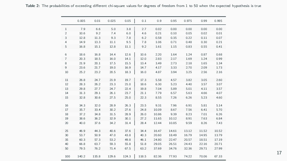
18. • Since there are four genotypic classes, we must use 4-1 = 3 degrees of freedom. • Consulting the χ2 table, we see our values of 9.88 and 3 df give a p value of ~0.025, or 2.5%. • This is less than the standard cut-off value of 5 percent, so we can reject the hypothesis of no linkage. • Hence, we are left with the conclusion that the genes are very likely linked, approximately 39 m.u. apart. 18
19. Bibliography 19
20. Reading materials For numerical analysis using χ2 test, See pp 96 of Griffiths et al. (2015). 20
21. References Griffiths, Anthony JF, Susan R Wessler, Sean B Carroll, Doebley John, and others. 2015. An Introduction to Genetic Analysis. Macmillan. 21