Upgrade to Pro — share decks privately, control downloads, hide ads and more …

jntushortnotes.blogspot.com -Jntuk engineering mathematics–1 (m1) materials

Dinesh
June 23, 2017

jntushortnotes.blogspot.com -Jntuk engineering mathematics–1 (m1) materials

Jntuk engineering mathematics–1 (m1) materials - jntushortnotes.blogspot.com
jntuk materials

Dinesh

June 23, 2017
Tweet

Other Decks in Education

Transcript

  1. Contents Preface xi Part 1 Number and Algebra 1 1

    Revision of fractions, decimals and percentages 1 1.1 Fractions 1 1.2 Ratio and proportion 3 1.3 Decimals 4 1.4 Percentages 7 2 Indices and standard form 9 2.1 Indices 9 2.2 Worked problems on indices 9 2.3 Further worked problems on indices 11 2.4 Standard form 13 2.5 Worked problems on standard form 13 2.6 Further worked problems on standard form 14 3 Computer numbering systems 16 3.1 Binary numbers 16 3.2 Conversion of binary to decimal 16 3.3 Conversion of decimal to binary 17 3.4 Conversion of decimal to binary via octal 18 3.5 Hexadecimal numbers 20 4 Calculations and evaluation of formulae 24 4.1 Errors and approximations 24 4.2 Use of calculator 26 4.3 Conversion tables and charts 28 4.4 Evaluation of formulae 30 Assignment 1 33 5 Algebra 34 5.1 Basic operations 34 5.2 Laws of Indices 36 5.3 Brackets and factorisation 38 5.4 Fundamental laws and precedence 40 5.5 Direct and inverse proportionality 42 6 Further algebra 44 6.1 Polynomial division 44 6.2 The factor theorem 46 6.3 The remainder theorem 48 7 Partial fractions 51 7.1 Introduction to partial fractions 51 7.2 Worked problems on partial fractions with linear factors 51 7.3 Worked problems on partial fractions with repeated linear factors 54 7.4 Worked problems on partial fractions with quadratic factors 55 8 Simple equations 57 8.1 Expressions, equations and identities 57 8.2 Worked problems on simple equations 57 8.3 Further worked problems on simple equations 59 8.4 Practical problems involving simple equations 61 8.5 Further practical problems involving simple equations 62 Assignment 2 64 9 Simultaneous equations 65 9.1 Introduction to simultaneous equations 65 9.2 Worked problems on simultaneous equations in two unknowns 65 9.3 Further worked problems on simultaneous equations 67 9.4 More difficult worked problems on simultaneous equations 69 9.5 Practical problems involving simultaneous equations 70 10 Transposition of formulae 74 10.1 Introduction to transposition of formulae 74 10.2 Worked problems on transposition of formulae 74 10.3 Further worked problems on transposition of formulae 75 10.4 Harder worked problems on transposition of formulae 77 11 Quadratic equations 80 11.1 Introduction to quadratic equations 80 11.2 Solution of quadratic equations by factorisation 80 alljntuworld.in JN TU W orld
  2. vi CONTENTS 11.3 Solution of quadratic equations by ‘completing the

    square’ 82 11.4 Solution of quadratic equations by formula 84 11.5 Practical problems involving quadratic equations 85 11.6 The solution of linear and quadratic equations simultaneously 87 12 Logarithms 89 12.1 Introduction to logarithms 89 12.2 Laws of logarithms 89 12.3 Indicial equations 92 12.4 Graphs of logarithmic functions 93 Assignment 3 94 13 Exponential functions 95 13.1 The exponential function 95 13.2 Evaluating exponential functions 95 13.3 The power series for ex 96 13.4 Graphs of exponential functions 98 13.5 Napierian logarithms 100 13.6 Evaluating Napierian logarithms 100 13.7 Laws of growth and decay 102 14 Number sequences 106 14.1 Arithmetic progressions 106 14.2 Worked problems on arithmetic progression 106 14.3 Further worked problems on arithmetic progressions 107 14.4 Geometric progressions 109 14.5 Worked problems on geometric progressions 110 14.6 Further worked problems on geometric progressions 111 14.7 Combinations and permutations 112 15 The binomial series 114 15.1 Pascal’s triangle 114 15.2 The binomial series 115 15.3 Worked problems on the binomial series 115 15.4 Further worked problems on the binomial series 117 15.5 Practical problems involving the binomial theorem 120 16 Solving equations by iterative methods 123 16.1 Introduction to iterative methods 123 16.2 The Newton–Raphson method 123 16.3 Worked problems on the Newton–Raphson method 123 Assignment 4 126 Multiple choice questions on chapters 1 to 16 127 Part 2 Mensuration 131 17 Areas of plane figures 131 17.1 Mensuration 131 17.2 Properties of quadrilaterals 131 17.3 Worked problems on areas of plane figures 132 17.4 Further worked problems on areas of plane figures 135 17.5 Worked problems on areas of composite figures 137 17.6 Areas of similar shapes 138 18 The circle and its properties 139 18.1 Introduction 139 18.2 Properties of circles 139 18.3 Arc length and area of a sector 140 18.4 Worked problems on arc length and sector of a circle 141 18.5 The equation of a circle 143 19 Volumes and surface areas of common solids 145 19.1 Volumes and surface areas of regular solids 145 19.2 Worked problems on volumes and surface areas of regular solids 145 19.3 Further worked problems on volumes and surface areas of regular solids 147 19.4 Volumes and surface areas of frusta of pyramids and cones 151 19.5 The frustum and zone of a sphere 155 19.6 Prismoidal rule 157 19.7 Volumes of similar shapes 159 20 Irregular areas and volumes and mean values of waveforms 161 20.1 Areas of irregular figures 161 20.2 Volumes of irregular solids 163 20.3 The mean or average value of a waveform 164 Assignment 5 168 Part 3 Trigonometry 171 21 Introduction to trigonometry 171 21.1 Trigonometry 171 21.2 The theorem of Pythagoras 171 21.3 Trigonometric ratios of acute angles 172 alljntuworld.in JN TU W orld
  3. CONTENTS vii 21.4 Fractional and surd forms of trigonometric ratios

    174 21.5 Solution of right-angled triangles 175 21.6 Angles of elevation and depression 176 21.7 Evaluating trigonometric ratios of any angles 178 21.8 Trigonometric approximations for small angles 181 22 Trigonometric waveforms 182 22.1 Graphs of trigonometric functions 182 22.2 Angles of any magnitude 182 22.3 The production of a sine and cosine wave 185 22.4 Sine and cosine curves 185 22.5 Sinusoidal form A sin ωt š ˛ 189 22.6 Waveform harmonics 192 23 Cartesian and polar co-ordinates 194 23.1 Introduction 194 23.2 Changing from Cartesian into polar co-ordinates 194 23.3 Changing from polar into Cartesian co-ordinates 196 23.4 Use of R ! P and P ! R functions on calculators 197 Assignment 6 198 24 Triangles and some practical applications 199 24.1 Sine and cosine rules 199 24.2 Area of any triangle 199 24.3 Worked problems on the solution of triangles and their areas 199 24.4 Further worked problems on the solution of triangles and their areas 201 24.5 Practical situations involving trigonometry 203 24.6 Further practical situations involving trigonometry 205 25 Trigonometric identities and equations 208 25.1 Trigonometric identities 208 25.2 Worked problems on trigonometric identities 208 25.3 Trigonometric equations 209 25.4 Worked problems (i) on trigonometric equations 210 25.5 Worked problems (ii) on trigonometric equations 211 25.6 Worked problems (iii) on trigonometric equations 212 25.7 Worked problems (iv) on trigonometric equations 212 26 Compound angles 214 26.1 Compound angle formulae 214 26.2 Conversion of a sin ωt C b cos ωt into R sin ωt C ˛) 216 26.3 Double angles 220 26.4 Changing products of sines and cosines into sums or differences 221 26.5 Changing sums or differences of sines and cosines into products 222 Assignment 7 224 Multiple choice questions on chapters 17 to 26 225 Part 4 Graphs 231 27 Straight line graphs 231 27.1 Introduction to graphs 231 27.2 The straight line graph 231 27.3 Practical problems involving straight line graphs 237 28 Reduction of non-linear laws to linear form 243 28.1 Determination of law 243 28.2 Determination of law involving logarithms 246 29 Graphs with logarithmic scales 251 29.1 Logarithmic scales 251 29.2 Graphs of the form y D axn 251 29.3 Graphs of the form y D abx 254 29.4 Graphs of the form y D aekx 255 30 Graphical solution of equations 258 30.1 Graphical solution of simultaneous equations 258 30.2 Graphical solution of quadratic equations 259 30.3 Graphical solution of linear and quadratic equations simultaneously 263 30.4 Graphical solution of cubic equations 264 31 Functions and their curves 266 31.1 Standard curves 266 31.2 Simple transformations 268 31.3 Periodic functions 273 31.4 Continuous and discontinuous functions 273 31.5 Even and odd functions 273 31.6 Inverse functions 275 Assignment 8 279 alljntuworld.in JN TU W orld
  4. viii CONTENTS Part 5 Vectors 281 32 Vectors 281 32.1

    Introduction 281 32.2 Vector addition 281 32.3 Resolution of vectors 283 32.4 Vector subtraction 284 33 Combination of waveforms 287 33.1 Combination of two periodic functions 287 33.2 Plotting periodic functions 287 33.3 Determining resultant phasors by calculation 288 Part 6 Complex Numbers 291 34 Complex numbers 291 34.1 Cartesian complex numbers 291 34.2 The Argand diagram 292 34.3 Addition and subtraction of complex numbers 292 34.4 Multiplication and division of complex numbers 293 34.5 Complex equations 295 34.6 The polar form of a complex number 296 34.7 Multiplication and division in polar form 298 34.8 Applications of complex numbers 299 35 De Moivre’s theorem 303 35.1 Introduction 303 35.2 Powers of complex numbers 303 35.3 Roots of complex numbers 304 Assignment 9 306 Part 7 Statistics 307 36 Presentation of statistical data 307 36.1 Some statistical terminology 307 36.2 Presentation of ungrouped data 308 36.3 Presentation of grouped data 312 37 Measures of central tendency and dispersion 319 37.1 Measures of central tendency 319 37.2 Mean, median and mode for discrete data 319 37.3 Mean, median and mode for grouped data 320 37.4 Standard deviation 322 37.5 Quartiles, deciles and percentiles 324 38 Probability 326 38.1 Introduction to probability 326 38.2 Laws of probability 326 38.3 Worked problems on probability 327 38.4 Further worked problems on probability 329 38.5 Permutations and combinations 331 39 The binomial and Poisson distribution 333 39.1 The binomial distribution 333 39.2 The Poisson distribution 336 Assignment 10 339 40 The normal distribution 340 40.1 Introduction to the normal distribution 340 40.2 Testing for a normal distribution 344 41 Linear correlation 347 41.1 Introduction to linear correlation 347 41.2 The product-moment formula for determining the linear correlation coefficient 347 41.3 The significance of a coefficient of correlation 348 41.4 Worked problems on linear correlation 348 42 Linear regression 351 42.1 Introduction to linear regression 351 42.2 The least-squares regression lines 351 42.3 Worked problems on linear regression 352 43 Sampling and estimation theories 356 43.1 Introduction 356 43.2 Sampling distributions 356 43.3 The sampling distribution of the means 356 43.4 The estimation of population parameters based on a large sample size 359 43.5 Estimating the mean of a population based on a small sample size 364 Assignment 11 368 Multiple choice questions on chapters 27 to 43 369 Part 8 Differential Calculus 375 44 Introduction to differentiation 375 44.1 Introduction to calculus 375 44.2 Functional notation 375 44.3 The gradient of a curve 376 44.4 Differentiation from first principles 377 alljntuworld.in JN TU W orld
  5. CONTENTS ix 44.5 Differentiation of y D axn by the

    general rule 379 44.6 Differentiation of sine and cosine functions 380 44.7 Differentiation of eax and ln ax 382 45 Methods of differentiation 384 45.1 Differentiation of common functions 384 45.2 Differentiation of a product 386 45.3 Differentiation of a quotient 387 45.4 Function of a function 389 45.5 Successive differentiation 390 46 Some applications of differentiation 392 46.1 Rates of change 392 46.2 Velocity and acceleration 393 46.3 Turning points 396 46.4 Practical problems involving maximum and minimum values 399 46.5 Tangents and normals 403 46.6 Small changes 404 Assignment 12 406 Part 9 Integral Calculus 407 47 Standard integration 407 47.1 The process of integration 407 47.2 The general solution of integrals of the form axn 407 47.3 Standard integrals 408 47.4 Definite integrals 411 48 Integration using algebraic substitutions 414 48.1 Introduction 414 48.2 Algebraic substitutions 414 48.3 Worked problems on integration using algebraic substitutions 414 48.4 Further worked problems on integration using algebraic substitutions 416 48.5 Change of limits 416 49 Integration using trigonometric substitutions 418 49.1 Introduction 418 49.2 Worked problems on integration of sin2 x, cos2 x, tan2 x and cot2 x 418 49.3 Worked problems on powers of sines and cosines 420 49.4 Worked problems on integration of products of sines and cosines 421 49.5 Worked problems on integration using the sin  substitution 422 49.6 Worked problems on integration using the tan  substitution 424 Assignment 13 425 50 Integration using partial fractions 426 50.1 Introduction 426 50.2 Worked problems on integration using partial fractions with linear factors 426 50.3 Worked problems on integration using partial fractions with repeated linear factors 427 50.4 Worked problems on integration using partial fractions with quadratic factors 428 51 The t = q 2 substitution 430 51.1 Introduction 430 51.2 Worked problems on the t D tan  2 substitution 430 51.3 Further worked problems on the t D tan  2 substitution 432 52 Integration by parts 434 52.1 Introduction 434 52.2 Worked problems on integration by parts 434 52.3 Further worked problems on integration by parts 436 53 Numerical integration 439 53.1 Introduction 439 53.2 The trapezoidal rule 439 53.3 The mid-ordinate rule 441 53.4 Simpson’s rule 443 Assignment 14 447 54 Areas under and between curves 448 54.1 Area under a curve 448 54.2 Worked problems on the area under a curve 449 54.3 Further worked problems on the area under a curve 452 54.4 The area between curves 454 55 Mean and root mean square values 457 55.1 Mean or average values 457 55.2 Root mean square values 459 56 Volumes of solids of revolution 461 56.1 Introduction 461 56.2 Worked problems on volumes of solids of revolution 461 alljntuworld.in JN TU W orld
  6. x CONTENTS 56.3 Further worked problems on volumes of solids

    of revolution 463 57 Centroids of simple shapes 466 57.1 Centroids 466 57.2 The first moment of area 466 57.3 Centroid of area between a curve and the x-axis 466 57.4 Centroid of area between a curve and the y-axis 467 57.5 Worked problems on centroids of simple shapes 467 57.6 Further worked problems on centroids of simple shapes 468 57.7 Theorem of Pappus 471 58 Second moments of area 475 58.1 Second moments of area and radius of gyration 475 58.2 Second moment of area of regular sections 475 58.3 Parallel axis theorem 475 58.4 Perpendicular axis theorem 476 58.5 Summary of derived results 476 58.6 Worked problems on second moments of area of regular sections 476 58.7 Worked problems on second moments of areas of composite areas 480 Assignment 15 482 Part 10 Further Number and Algebra 483 59 Boolean algebra and logic circuits 483 59.1 Boolean algebra and switching circuits 483 59.2 Simplifying Boolean expressions 488 59.3 Laws and rules of Boolean algebra 488 59.4 De Morgan’s laws 490 59.5 Karnaugh maps 491 59.6 Logic circuits 495 59.7 Universal logic circuits 500 60 The theory of matrices and determinants 504 60.1 Matrix notation 504 60.2 Addition, subtraction and multiplication of matrices 504 60.3 The unit matrix 508 60.4 The determinant of a 2 by 2 matrix 508 60.5 The inverse or reciprocal of a 2 by 2 matrix 509 60.6 The determinant of a 3 by 3 matrix 510 60.7 The inverse or reciprocal of a 3 by 3 matrix 511 61 The solution of simultaneous equations by matrices and determinants 514 61.1 Solution of simultaneous equations by matrices 514 61.2 Solution of simultaneous equations by determinants 516 61.3 Solution of simultaneous equations using Cramers rule 520 Assignment 16 521 Multiple choice questions on chapters 44–61 522 Answers to multiple choice questions 526 Index 527 alljntuworld.in JN TU W orld
  7. Preface This fourth edition of ‘Engineering Mathematics’ covers a wide

    range of syllabus requirements. In particular, the book is most suitable for the latest National Certificate and Diploma courses and Vocational Certificate of Education syllabuses in Engineering. This text will provide a foundation in mathematical principles, which will enable students to solve mathe- matical, scientific and associated engineering princi- ples. In addition, the material will provide engineer- ing applications and mathematical principles neces- sary for advancement onto a range of Incorporated Engineer degree profiles. It is widely recognised that a students’ ability to use mathematics is a key element in determining subsequent success. First year under- graduates who need some remedial mathematics will also find this book meets their needs. In Engineering Mathematics 4th Edition, theory is introduced in each chapter by a simple outline of essential definitions, formulae, laws and procedures. The theory is kept to a minimum, for problem solv- ing is extensively used to establish and exemplify the theory. It is intended that readers will gain real understanding through seeing problems solved and then through solving similar problems themselves. For clarity, the text is divided into ten topic areas, these being: number and algebra, mensura- tion, trigonometry, graphs, vectors, complex num- bers, statistics, differential calculus, integral calculus and further number and algebra. This new edition will cover the following syl- labuses: (i) Mathematics for Technicians, the core unit for National Certificate/Diploma courses in Engineering, to include all or part of the following chapters: 1. Algebra: 2, 4, 5, 8–13, 17, 19, 27, 30 2. Trigonometry: 18, 21, 22, 24 3. Statistics: 36, 37 4. Calculus: 44, 46, 47, 54 (ii) Further Mathematics for Technicians, the optional unit for National Certifi- cate/Diploma courses in Engineering, to include all or part of the following chapters: 1. Algebraic techniques: 10, 14, 15, 28–30, 34, 59–61 2. Trigonometry: 22–24, 26 3. Calculus: 44–49, 52–58 4. Statistical and probability: 36–43 (iii) Applied Mathematics in Engineering, the compulsory unit for Advanced VCE (for- merly Advanced GNVQ), to include all or part of the following chapters: 1. Number and units: 1, 2, 4 2. Mensuration: 17–20 3. Algebra: 5, 8–11 4. Functions and graphs: 22, 23, 27 5. Trigonometry: 21, 24 (iv) Further Mathematics for Engineering, the optional unit for Advanced VCE (formerly Advanced GNVQ), to include all or part of the following chapters: 1. Algebra and trigonometry: 5, 6, 12–15, 21, 25 2. Graphical and numerical techniques: 20, 22, 26–31 3. Differential and integral calculus: 44–47, 54 (v) The Mathematics content of Applied Sci- ence and Mathematics for Engineering, for Intermediate GNVQ (vi) Mathematics for Engineering, for Founda- tion and Intermediate GNVQ (vii) Mathematics 2 and Mathematics 3 for City & Guilds Technician Diploma in Telecom- munications and Electronic Engineering (viii) Any introductory/access/foundation co- urse involving Engineering Mathematics at University, Colleges of Further and Higher education and in schools. Each topic considered in the text is presented in a way that assumes in the reader little previous knowledge of that topic. alljntuworld.in JN TU W orld
  8. xii ENGINEERING MATHEMATICS ‘Engineering Mathematics 4th Edition’ provides a follow-up

    to ‘Basic Engineering Mathematics’ and a lead into ‘Higher Engineering Mathemat- ics’. This textbook contains over 900 worked problems, followed by some 1700 further problems (all with answers). The further problems are contained within some 208 Exercises; each Exercise follows on directly from the relevant section of work, every two or three pages. In addition, the text contains 234 multiple-choice questions. Where at all possible, the problems mirror practical situations found in engineering and science. 500 line diagrams enhance the understanding of the theory. At regular intervals throughout the text are some 16 Assignments to check understanding. For exam- ple, Assignment 1 covers material contained in Chapters 1 to 4, Assignment 2 covers the material in Chapters 5 to 8, and so on. These Assignments do not have answers given since it is envisaged that lecturers could set the Assignments for students to attempt as part of their course structure. Lecturers’ may obtain a complimentary set of solutions of the Assignments in an Instructor’s Manual available from the publishers via the internet — full worked solutions and mark scheme for all the Assignments are contained in this Manual, which is available to lecturers only. To obtain a password please e-mail [email protected] with the following details: course title, number of students, your job title and work postal address. To download the Instructor’s Manual visit http://www.newnespress.com and enter the book title in the search box, or use the following direct URL: http://www.bh.com/manuals/0750657766/ ‘Learning by Example’ is at the heart of ‘Engi- neering Mathematics 4th Edition’. John Bird University of Portsmouth alljntuworld.in JN TU W orld
  9. Part 1 Number and Algebra 1 Revision of fractions, decimals

    and percentages 1.1 Fractions When 2 is divided by 3, it may be written as 2 3 or 2/3. 2 3 is called a fraction. The number above the line, i.e. 2, is called the numerator and the number below the line, i.e. 3, is called the denominator. When the value of the numerator is less than the value of the denominator, the fraction is called a proper fraction; thus 2 3 is a proper fraction. When the value of the numerator is greater than the denominator, the fraction is called an improper fraction. Thus 7 3 is an improper fraction and can also be expressed as a mixed number, that is, an integer and a proper fraction. Thus the improper fraction 7 3 is equal to the mixed number 21 3 . When a fraction is simplified by dividing the numerator and denominator by the same number, the process is called cancelling. Cancelling by 0 is not permissible. Problem 1. Simplify 1 3 C 2 7 The lowest common multiple (i.e. LCM) of the two denominators is 3 ð 7, i.e. 21 Expressing each fraction so that their denomina- tors are 21, gives: 1 3 C 2 7 D 1 3 ð 7 7 C 2 7 ð 3 3 D 7 21 C 6 21 D 7 C 6 21 D 13 21 Alternatively: 1 3 C 2 7 D Step (2) # 7 ð 1 C Step (3) # 3 ð 2 21 " Step (1) Step 1: the LCM of the two denominators; Step 2: for the fraction 1 3 , 3 into 21 goes 7 times, 7 ð the numerator is 7 ð 1; Step 3: for the fraction 2 7 , 7 into 21 goes 3 times, 3 ð the numerator is 3 ð 2. Thus 1 3 C 2 7 D 7 C 6 21 D 13 21 as obtained previously. Problem 2. Find the value of 3 2 3 2 1 6 One method is to split the mixed numbers into integers and their fractional parts. Then 3 2 3 2 1 6 D 3 C 2 3 2 C 1 6 D 3 C 2 3 2 1 6 D 1 C 4 6 1 6 D 1 3 6 D 1 1 2 Another method is to express the mixed numbers as improper fractions. alljntuworld.in JN TU W orld
  10. 2 ENGINEERING MATHEMATICS Since 3 D 9 3 , then

    3 2 3 D 9 3 C 2 3 D 11 3 Similarly, 2 1 6 D 12 6 C 1 6 D 13 6 Thus 3 2 3 2 1 6 D 11 3 13 6 D 22 6 13 6 D 9 6 D 1 1 2 as obtained previously. Problem 3. Determine the value of 4 5 8 3 1 4 C 1 2 5 4 5 8 3 1 4 C 1 2 5 D 4 3 C 1 C 5 8 1 4 C 2 5 D 2 C 5 ð 5 10 ð 1 C 8 ð 2 40 D 2 C 25 10 C 16 40 D 2 C 31 40 D 2 31 40 Problem 4. Find the value of 3 7 ð 14 15 Dividing numerator and denominator by 3 gives: 1 3 7 ð 14 15 5 D 1 7 ð 14 5 D 1 ð 14 7 ð 5 Dividing numerator and denominator by 7 gives: 1 ð 14 2 1 7 ð 5 D 1 ð 2 1 ð 5 D 2 5 This process of dividing both the numerator and denominator of a fraction by the same factor(s) is called cancelling. Problem 5. Evaluate 1 3 5 ð 2 1 3 ð 3 3 7 Mixed numbers must be expressed as improper fractions before multiplication can be performed. Thus, 1 3 5 ð 2 1 3 ð 3 3 7 D 5 5 C 3 5 ð 6 3 C 1 3 ð 21 7 C 3 7 D 8 5 ð 1 7 1 3 ð 24 8 71 D 8 ð 1 ð 8 5 ð 1 ð 1 D 64 5 D 12 4 5 Problem 6. Simplify 3 7 ł 12 21 3 7 ł 12 21 D 3 7 12 21 Multiplying both numerator and denominator by the reciprocal of the denominator gives: 3 7 12 21 D 1 3 1 7 ð 21 3 12 4 1 12 1 21 ð 21 1 12 1 D 3 4 1 D 3 4 This method can be remembered by the rule: invert the second fraction and change the operation from division to multiplication. Thus: 3 7 ł 12 21 D 1 3 1 7 ð 21 3 12 4 D 3 4 as obtained previously. Problem 7. Find the value of 5 3 5 ł 7 1 3 The mixed numbers must be expressed as improper fractions. Thus, 5 3 5 ł 7 1 3 D 28 5 ł 22 3 D 14 28 5 ð 3 22 11 D 42 55 Problem 8. Simplify 1 3 2 5 C 1 4 ł 3 8 ð 1 3 The order of precedence of operations for problems containing fractions is the same as that for inte- gers, i.e. remembered by BODMAS (Brackets, Of, Division, Multiplication, Addition and Subtraction). Thus, 1 3 2 5 C 1 4 ł 3 8 ð 1 3 alljntuworld.in JN TU W orld
  11. REVISION OF FRACTIONS, DECIMALS AND PERCENTAGES 3 D 1 3

    4 ð 2 C 5 ð 1 20 ł 31 24 8 (B) D 1 3 13 5 20 ð 82 1 (D) D 1 3 26 5 (M) D 5 ð 1 3 ð 26 15 (S) D 73 15 D −4 13 15 Problem 9. Determine the value of 7 6 of 3 1 2 2 1 4 C 5 1 8 ł 3 16 1 2 7 6 of 3 1 2 2 1 4 C 5 1 8 ł 3 16 1 2 D 7 6 of 1 1 4 C 41 8 ł 3 16 1 2 (B) D 7 6 ð 5 4 C 41 8 ł 3 16 1 2 (O) D 7 6 ð 5 4 C 41 1 8 ð 16 2 3 1 2 (D) D 35 24 C 82 3 1 2 (M) D 35 C 656 24 1 2 (A) D 691 24 1 2 (A) D 691 12 24 (S) D 679 24 D 28 7 24 Now try the following exercise Exercise 1 Further problems on fractions Evaluate the following: 1. (a) 1 2 C 2 5 (b) 7 16 1 4 (a) 9 10 (b) 3 16 2. (a) 2 7 C 3 11 (b) 2 9 1 7 C 2 3 (a) 43 77 (b) 47 63 3. (a) 10 3 7 8 2 3 (b) 3 1 4 4 4 5 C 1 5 6 (a) 1 16 21 (b) 17 60 4. (a) 3 4 ð 5 9 (b) 17 35 ð 15 119 (a) 5 12 (b) 3 49 5. (a) 3 5 ð 7 9 ð 1 2 7 (b) 13 17 ð 4 7 11 ð 3 4 39 (a) 3 5 (b) 11 6. (a) 3 8 ł 45 64 (b) 1 1 3 ł 2 5 9 (a) 8 15 (b) 12 23 7. 1 2 C 3 5 ł 8 15 1 3 1 7 24 8. 7 15 of 15 ð 5 7 C 3 4 ł 15 16 5 4 5 9. 1 4 ð 2 3 1 3 ł 3 5 C 2 7 13 126 10. 2 3 ð 1 1 4 ł 2 3 C 1 4 C 1 3 5 2 28 55 1.2 Ratio and proportion The ratio of one quantity to another is a fraction, and is the number of times one quantity is contained in another quantity of the same kind. If one quantity is directly proportional to another, then as one quan- tity doubles, the other quantity also doubles. When a quantity is inversely proportional to another, then as one quantity doubles, the other quantity is halved. Problem 10. A piece of timber 273 cm long is cut into three pieces in the ratio of 3 to 7 to 11. Determine the lengths of the three pieces alljntuworld.in JN TU W orld
  12. 4 ENGINEERING MATHEMATICS The total number of parts is 3

    C 7 C 11, that is, 21. Hence 21 parts correspond to 273 cm 1 part corresponds to 273 21 D 13 cm 3 parts correspond to 3 ð 13 D 39 cm 7 parts correspond to 7 ð 13 D 91 cm 11 parts correspond to 11 ð 13 D 143 cm i.e. the lengths of the three pieces are 39 cm, 91 cm and 143 cm. (Check: 39 C 91 C 143 D 273) Problem 11. A gear wheel having 80 teeth is in mesh with a 25 tooth gear. What is the gear ratio? Gear ratio D 80:25 D 80 25 D 16 5 D 3.2 i.e. gear ratio D 16 : 5 or 3.2 : 1 Problem 12. An alloy is made up of metals A and B in the ratio 2.5 : 1 by mass. How much of A has to be added to 6 kg of B to make the alloy? Ratio A : B: :2.5 : 1 (i.e. A is to B as 2.5 is to 1) or A B D 2.5 1 D 2.5 When B D 6 kg, A 6 D 2.5 from which, A D 6 ð 2.5 D 15 kg Problem 13. If 3 people can complete a task in 4 hours, how long will it take 5 people to complete the same task, assuming the rate of work remains constant The more the number of people, the more quickly the task is done, hence inverse proportion exists. 3 people complete the task in 4 hours, 1 person takes three times as long, i.e. 4 ð 3 D 12 hours, 5 people can do it in one fifth of the time that one person takes, that is 12 5 hours or 2 hours 24 minutes. Now try the following exercise Exercise 5 Further problems on ratio and proportion 1. Divide 621 cm in the ratio of 3 to 7 to 13. [81 cm to 189 cm to 351 cm] 2. When mixing a quantity of paints, dyes of four different colours are used in the ratio of 7:3:19:5. If the mass of the first dye used is 31 2 g, determine the total mass of the dyes used. [17 g] 3. Determine how much copper and how much zinc is needed to make a 99 kg brass ingot if they have to be in the proportions copper : zinc: :8 : 3 by mass. [72 kg : 27 kg] 4. It takes 21 hours for 12 men to resurface a stretch of road. Find how many men it takes to resurface a similar stretch of road in 50 hours 24 minutes, assuming the work rate remains constant. [5] 5. It takes 3 hours 15 minutes to fly from city A to city B at a constant speed. Find how long the journey takes if (a) the speed is 11 2 times that of the original speed and (b) if the speed is three-quarters of the original speed. [(a) 2 h 10 min (b) 4 h 20 min] 1.3 Decimals The decimal system of numbers is based on the digits 0 to 9. A number such as 53.17 is called a decimal fraction, a decimal point separating the integer part, i.e. 53, from the fractional part, i.e. 0.17 alljntuworld.in JN TU W orld
  13. REVISION OF FRACTIONS, DECIMALS AND PERCENTAGES 5 A number which

    can be expressed exactly as a decimal fraction is called a terminating deci- mal and those which cannot be expressed exactly as a decimal fraction are called non-terminating decimals. Thus, 3 2 D 1.5 is a terminating decimal, but 4 3 D 1.33333. . . is a non-terminating decimal. 1.33333. . . can be written as 1.P 3, called ‘one point- three recurring’. The answer to a non-terminating decimal may be expressed in two ways, depending on the accuracy required: (i) correct to a number of significant figures, that is, figures which signify something, and (ii) correct to a number of decimal places, that is, the number of figures after the decimal point. The last digit in the answer is unaltered if the next digit on the right is in the group of numbers 0, 1, 2, 3 or 4, but is increased by 1 if the next digit on the right is in the group of numbers 5, 6, 7, 8 or 9. Thus the non-terminating decimal 7.6183. . . becomes 7.62, correct to 3 significant figures, since the next digit on the right is 8, which is in the group of numbers 5, 6, 7, 8 or 9. Also 7.6183. . . becomes 7.618, correct to 3 decimal places, since the next digit on the right is 3, which is in the group of numbers 0, 1, 2, 3 or 4. Problem 14. Evaluate 42.7 C 3.04 C 8.7 C 0.06 The numbers are written so that the decimal points are under each other. Each column is added, starting from the right. 42.7 3.04 8.7 0.06 54.50 Thus 42.7 Y 3.04 Y 8.7 Y 0.06 = 54.50 Problem 15. Take 81.70 from 87.23 The numbers are written with the decimal points under each other. 87.23 81.70 5.53 Thus 87.23 − 81.70 = 5.53 Problem 16. Find the value of 23.4 17.83 57.6 C 32.68 The sum of the positive decimal fractions is 23.4 C 32.68 D 56.08 The sum of the negative decimal fractions is 17.83 C 57.6 D 75.43 Taking the sum of the negative decimal fractions from the sum of the positive decimal fractions gives: 56.08 75.43 i.e. 75.43 56.08 D −19.35 Problem 17. Determine the value of 74.3 ð 3.8 When multiplying decimal fractions: (i) the numbers are multiplied as if they are integers, and (ii) the position of the decimal point in the answer is such that there are as many digits to the right of it as the sum of the digits to the right of the decimal points of the two numbers being multiplied together. Thus (i) 743 38 5 944 22 290 28 234 (ii) As there are 1 C 1 D 2 digits to the right of the decimal points of the two numbers being multiplied together, (74.3 ð 3.8), then 74.3 × 3.8 = 282.34 Problem 18. Evaluate 37.81 ł 1.7, correct to (i) 4 significant figures and (ii) 4 decimal places alljntuworld.in JN TU W orld
  14. 6 ENGINEERING MATHEMATICS 37.81 ł 1.7 D 37.81 1.7 The

    denominator is changed into an integer by multiplying by 10. The numerator is also multiplied by 10 to keep the fraction the same. Thus 37.81 ł 1.7 D 37.81 ð 10 1.7 ð 10 D 378.1 17 The long division is similar to the long division of integers and the first four steps are as shown: 22.24117.. 17 378.100000 34 38 34 41 34 70 68 20 (i) 37.81 ÷ 1.7 = 22.24, correct to 4 significant figures, and (ii) 37.81 ÷ 1.7 = 22.2412, correct to 4 decimal places. Problem 19. Convert (a) 0.4375 to a proper fraction and (b) 4.285 to a mixed number (a) 0.4375 can be written as 0.4375 ð 10 000 10 000 without changing its value, i.e. 0.4375 D 4375 10 000 By cancelling 4375 10 000 D 875 2000 D 175 400 D 35 80 D 7 16 i.e. 0.4375 = 7 16 (b) Similarly, 4.285 D 4 285 1000 D 4 57 200 Problem 20. Express as decimal fractions: (a) 9 16 and (b) 5 7 8 (a) To convert a proper fraction to a decimal frac- tion, the numerator is divided by the denomi- nator. Division by 16 can be done by the long division method, or, more simply, by dividing by 2 and then 8: 4.50 2 9.00 0.5625 8 4.5000 Thus, 9 16 = 0.5625 (b) For mixed numbers, it is only necessary to convert the proper fraction part of the mixed number to a decimal fraction. Thus, dealing with the 7 8 gives: 0.875 8 7.000 i.e. 7 8 D 0.875 Thus 5 7 8 = 5.875 Now try the following exercise Exercise 3 Further problems on decimals In Problems 1 to 6, determine the values of the expressions given: 1. 23.6 C 14.71 18.9 7.421 [11.989] 2. 73.84 113.247 C 8.21 0.068 [ 31.265] 3. 3.8 ð 4.1 ð 0.7 [10.906] 4. 374.1 ð 0.006 [2.2446] 5. 421.8 ł 17, (a) correct to 4 significant figures and (b) correct to 3 decimal places. [(a) 24.81 (b) 24.812] 6. 0.0147 2.3 , (a) correct to 5 decimal places and (b) correct to 2 significant figures. [(a) 0.00639 (b) 0.0064] alljntuworld.in JN TU W orld
  15. REVISION OF FRACTIONS, DECIMALS AND PERCENTAGES 7 7. Convert to

    proper fractions: (a) 0.65 (b) 0.84 (c) 0.0125 (d) 0.282 and (e) 0.024 (a) 13 20 (b) 21 25 (c) 1 80 (d) 141 500 (e) 3 125 8. Convert to mixed numbers: (a) 1.82 (b) 4.275 (c) 14.125 (d) 15.35 and (e) 16.2125     (a) 1 41 50 (b) 4 11 40 (c) 14 1 8 (d) 15 7 20 (e) 16 17 80     In Problems 9 to 12, express as decimal frac- tions to the accuracy stated: 9. 4 9 , correct to 5 significant figures. [0.44444] 10. 17 27 , correct to 5 decimal place. [0.62963] 11. 1 9 16 , correct to 4 significant figures. [1.563] 12. 13 31 37 , correct to 2 decimal places. [13.84] 1.4 Percentages Percentages are used to give a common standard and are fractions having the number 100 as their denominators. For example, 25 per cent means 25 100 i.e. 1 4 and is written 25%. Problem 21. Express as percentages: (a) 1.875 and (b) 0.0125 A decimal fraction is converted to a percentage by multiplying by 100. Thus, (a) 1.875 corresponds to 1.875 ð 100%, i.e. 187.5% (b) 0.0125 corresponds to 0.0125 ð 100%, i.e. 1.25% Problem 22. Express as percentages: (a) 5 16 and (b) 1 2 5 To convert fractions to percentages, they are (i) con- verted to decimal fractions and (ii) multiplied by 100 (a) By division, 5 16 D 0.3125, hence 5 16 corre- sponds to 0.3125 ð 100%, i.e. 31.25% (b) Similarly, 1 2 5 D 1.4 when expressed as a decimal fraction. Hence 1 2 5 D 1.4 ð 100% D 140% Problem 23. It takes 50 minutes to machine a certain part. Using a new type of tool, the time can be reduced by 15%. Calculate the new time taken 15% of 50 minutes D 15 100 ð 50 D 750 100 D 7.5 minutes. hence the new time taken is 50 7.5 D 42.5 minutes. Alternatively, if the time is reduced by 15%, then it now takes 85% of the original time, i.e. 85% of 50 D 85 100 ð 50 D 4250 100 D 42.5 minutes, as above. Problem 24. Find 12.5% of £378 12.5% of £378 means 12.5 100 ð 378, since per cent means ‘per hundred’. Hence 12.5% of £378 D 12.51 100 8 ð 378 D 1 8 ð 378 D 378 8 D £47.25 alljntuworld.in JN TU W orld
  16. 8 ENGINEERING MATHEMATICS Problem 25. Express 25 minutes as a

    percentage of 2 hours, correct to the nearest 1% Working in minute units, 2 hours D 120 minutes. Hence 25 minutes is 25 120 ths of 2 hours. By can- celling, 25 120 D 5 24 Expressing 5 24 as a decimal fraction gives 0.208P 3 Multiplying by 100 to convert the decimal fraction to a percentage gives: 0.208P 3 ð 100 D 20.8P 3% Thus 25 minutes is 21% of 2 hours, correct to the nearest 1%. Problem 26. A German silver alloy consists of 60% copper, 25% zinc and 15% nickel. Determine the masses of the copper, zinc and nickel in a 3.74 kilogram block of the alloy By direct proportion: 100% corresponds to 3.74 kg 1% corresponds to 3.74 100 D 0.0374 kg 60% corresponds to 60 ð 0.0374 D 2.244 kg 25% corresponds to 25 ð 0.0374 D 0.935 kg 15% corresponds to 15 ð 0.0374 D 0.561 kg Thus, the masses of the copper, zinc and nickel are 2.244 kg, 0.935 kg and 0.561 kg, respectively. (Check: 2.244 C 0.935 C 0.561 D 3.74) Now try the following exercise Exercise 4 Further problems percentages 1. Convert to percentages: (a) 0.057 (b) 0.374 (c) 1.285 [(a) 5.7% (b) 37.4% (c) 128.5%] 2. Express as percentages, correct to 3 significant figures: (a) 7 33 (b) 19 24 (c) 1 11 16 [(a) 21.2% (b) 79.2% (c) 169%] 3. Calculate correct to 4 significant figures: (a) 18% of 2758 tonnes (b) 47% of 18.42 grams (c) 147% of 14.1 seconds [(a) 496.4 t (b) 8.657 g (c) 20.73 s] 4. When 1600 bolts are manufactured, 36 are unsatisfactory. Determine the percent- age unsatisfactory. [2.25%] 5. Express: (a) 140 kg as a percentage of 1 t (b) 47 s as a percentage of 5 min (c) 13.4 cm as a percentage of 2.5 m [(a) 14% (b) 15.67% (c) 5.36%] 6. A block of monel alloy consists of 70% nickel and 30% copper. If it contains 88.2 g of nickel, determine the mass of copper in the block. [37.8 g] 7. A drilling machine should be set to 250 rev/min. The nearest speed available on the machine is 268 rev/min. Calculate the percentage over speed. [7.2%] 8. Two kilograms of a compound contains 30% of element A, 45% of element B and 25% of element C. Determine the masses of the three elements present. [A 0.6 kg, B 0.9 kg, C 0.5 kg] 9. A concrete mixture contains seven parts by volume of ballast, four parts by vol- ume of sand and two parts by volume of cement. Determine the percentage of each of these three constituents correct to the nearest 1% and the mass of cement in a two tonne dry mix, correct to 1 significant figure. [54%, 31%, 15%, 0.3 t] alljntuworld.in JN TU W orld
  17. 2 Indices and standard form 2.1 Indices The lowest factors

    of 2000 are 2ð2ð2ð2ð5ð5ð5. These factors are written as 24 ð 53, where 2 and 5 are called bases and the numbers 4 and 3 are called indices. When an index is an integer it is called a power. Thus, 24 is called ‘two to the power of four’, and has a base of 2 and an index of 4. Similarly, 53 is called ‘five to the power of 3’ and has a base of 5 and an index of 3. Special names may be used when the indices are 2 and 3, these being called ‘squared’ and ‘cubed’, respectively. Thus 72 is called ‘seven squared’ and 93 is called ‘nine cubed’. When no index is shown, the power is 1, i.e. 2 means 21. Reciprocal The reciprocal of a number is when the index is 1 and its value is given by 1, divided by the base. Thus the reciprocal of 2 is 2 1 and its value is 1 2 or 0.5. Similarly, the reciprocal of 5 is 5 1 which means 1 5 or 0.2 Square root The square root of a number is when the index is 1 2 , and the square root of 2 is written as 21/2 or p 2. The value of a square root is the value of the base which when multiplied by itself gives the number. Since 3ð3 D 9, then p 9 D 3. However, 3 ð 3 D 9, so p 9 D 3. There are always two answers when finding the square root of a number and this is shown by putting both a C and a sign in front of the answer to a square root problem. Thus p 9 D š3 and 41/2 D p 4 D š2, and so on. Laws of indices When simplifying calculations involving indices, certain basic rules or laws can be applied, called the laws of indices. These are given below. (i) When multiplying two or more numbers hav- ing the same base, the indices are added. Thus 32 ð 34 D 32C4 D 36 (ii) When a number is divided by a number having the same base, the indices are subtracted. Thus 35 32 D 35 2 D 33 (iii) When a number which is raised to a power is raised to a further power, the indices are multiplied. Thus 35 2 D 35ð2 D 310 (iv) When a number has an index of 0, its value is 1. Thus 30 D 1 (v) A number raised to a negative power is the reciprocal of that number raised to a positive power. Thus 3 4 D 1 34 Similarly, 1 2 3 D 23 (vi) When a number is raised to a fractional power the denominator of the fraction is the root of the number and the numerator is the power. Thus 82/3 D 3 p 82 D 2 2 D 4 and 251/2 D 2 p 251 D p 251 D š5 (Note that p Á 2 p ) 2.2 Worked problems on indices Problem 1. Evaluate: (a) 52 ð 53, (b) 32 ð 34 ð 3 and (c) 2 ð 22 ð 25 From law (i): (a) 52ð53 D 5 2C3 D 55 D 5ð5ð5ð5ð5 D 3125 alljntuworld.in JN TU W orld
  18. 10 ENGINEERING MATHEMATICS (b) 32 ð 34 ð 3 D

    3 2C4C1 D 37 D 3 ð 3 ð Ð Ð Ð to 7 terms D 2187 (c) 2 ð 22 ð 25 D 2 1C2C5 D 28 D 256 Problem 2. Find the value of: (a) 75 73 and (b) 57 54 From law (ii): (a) 75 73 D 7 5 3 D 72 D 49 (b) 57 54 D 5 7 4 D 53 D 125 Problem 3. Evaluate: (a) 52 ð 53 ł 54 and (b) 3 ð 35 ł 32 ð 33 From laws (i) and (ii): (a) 52 ð 53 ł 54 D 52 ð 53 54 D 5 2C3 54 D 55 54 D 5 5 4 D 51 D 5 (b) 3 ð 35 ł 32 ð 33 D 3 ð 35 32 ð 33 D 3 1C5 3 2C3 D 36 35 D 36 5 D 31 D 3 Problem 4. Simplify: (a) 23 4 (b) 32 5, expressing the answers in index form. From law (iii): (a) 23 4 D 23ð4 D 212 (b) 32 5 D 32ð5 D 310 Problem 5. Evaluate: 102 3 104 ð 102 From the laws of indices: 102 3 104 ð 102 D 10 2ð3 10 4C2 D 106 106 D 106 6 D 100 D 1 Problem 6. Find the value of (a) 23 ð 24 27 ð 25 and (b) 32 3 3 ð 39 From the laws of indices: (a) 23 ð 24 27 ð 25 D 2 3C4 2 7C5 D 27 212 D 27 12 D 2 5 D 1 25 D 1 32 (b) 32 3 3 ð 39 D 32ð3 31C9 D 36 310 D 36 10 D 3 4 D 1 34 D 1 81 Now try the following exercise Exercise 5 Further problems on indices In Problems 1 to 10, simplify the expressions given, expressing the answers in index form and with positive indices: 1. (a) 33 ð 34 (b) 42 ð 43 ð 44 [(a) 37 (b) 49] 2. (a) 23 ð 2 ð 22 (b) 72 ð 74 ð 7 ð 73 [(a) 26 (b) 710] 3. (a) 24 23 (b) 37 32 [(a) 2 (b) 35] 4. (a) 56 ł 53 (b) 713/710 [(a) 53 (b) 73] 5. (a) 72 3 (b) 33 2 [(a) 76 (b) 36] 6. (a) 22 ð 23 24 (b) 37 ð 34 35 [(a) 2 (b) 36] 7. (a) 57 52 ð 53 (b) 135 13 ð 132 [(a) 52 (b) 132] 8. (a) 9 ð 32 3 3 ð 27 2 (b) 16 ð 4 2 2 ð 8 3 [(a) 34 (b) 1] alljntuworld.in JN TU W orld
  19. INDICES AND STANDARD FORM 11 9. (a) 5 2 5

    4 (b) 32 ð 3 4 33 (a) 52 (b) 1 35 10. (a) 72 ð 7 3 7 ð 7 4 (b) 23 ð 2 4 ð 25 2 ð 2 2 ð 26 (a) 72 (b) 1 2 2.3 Further worked problems on indices Problem 7. Evaluate: 33 ð 57 53 ð 34 The laws of indices only apply to terms having the same base. Grouping terms having the same base, and then applying the laws of indices to each of the groups independently gives: 33 ð 57 53 ð 34 D 33 34 ð 57 53 D 3 3 4 ð 5 7 3 D 3 1 ð 54 D 54 31 D 625 3 D 208 1 3 Problem 8. Find the value of 23 ð 35 ð 72 2 74 ð 24 ð 33 23 ð 35 ð 72 2 74 ð 24 ð 33 D 23 4 ð 35 3 ð 72ð2 4 D 2 1 ð 32 ð 70 D 1 2 ð 32 ð 1 D 9 2 D 4 1 2 Problem 9. Evaluate: (a) 41/2 (b) 163/4 (c) 272/3 (d) 9 1/2 (a) 41/2 D p 4 D ±2 (b) 163/4 D 4 p 163 D š2 3 D ±8 (Note that it does not matter whether the 4th root of 16 is found first or whether 16 cubed is found first — the same answer will result). (c) 272/3 D 3 p 272 D 3 2 D 9 (d) 9 1/2 D 1 91/2 D 1 p 9 D 1 š3 D ± 1 3 Problem 10. Evaluate: 41.5 ð 81/3 22 ð 32 2/5 41.5 D 43/2 D p 43 D 23 D 8, 81/3 D 3 p 8 D 2, 22 D 4 and 32 2/5 D 1 322/5 D 1 5 p 322 D 1 22 D 1 4 Hence 41.5 ð 81/3 22 ð 32 2/5 D 8 ð 2 4 ð 1 4 D 16 1 D 16 Alternatively, 41.5 ð 81/3 22 ð 32 2/5 D [ 2 2]3/2 ð 23 1/3 22 ð 25 2/5 D 23 ð 21 22 ð 2 2 D 23C1 2 2 D 24 D 16 Problem 11. Evaluate: 32 ð 55 C 33 ð 53 34 ð 54 Dividing each term by the HCF (i.e. highest com- mon factor) of the three terms, i.e. 32 ð 53, gives: 32 ð 55 C 33 ð 53 34 ð 54 D 32 ð 55 32 ð 53 C 33 ð 53 32 ð 53 34 ð 54 32 ð 53 D 3 2 2 ð 5 5 3 C 3 3 2 ð 50 3 4 2 ð 5 4 3 D 30 ð 52 C 31 ð 50 32 ð 51 D 1 ð 25 C 3 ð 1 9 ð 5 D 28 45 Problem 12. Find the value of 32 ð 55 34 ð 54 C 33 ð 53 alljntuworld.in JN TU W orld
  20. 12 ENGINEERING MATHEMATICS To simplify the arithmetic, each term is

    divided by the HCF of all the terms, i.e. 32 ð 53. Thus 32 ð 55 34 ð 54 C 33 ð 53 D 32 ð 55 32 ð 53 34 ð 54 32 ð 53 C 33 ð 53 32 ð 53 D 3 2 2 ð 5 5 3 3 4 2 ð 5 4 3 C 3 3 2 ð 5 3 3 D 30 ð 52 32 ð 51 C 31 ð 50 D 25 45 C 3 D 25 48 Problem 13. Simplify: 4 3 3 ð 3 5 2 2 5 3 giving the answer with positive indices A fraction raised to a power means that both the numerator and the denominator of the fraction are raised to that power, i.e. 4 3 3 D 43 33 A fraction raised to a negative power has the same value as the inverse of the fraction raised to a positive power. Thus, 3 5 2 D 1 3 5 2 D 1 32 52 D 1 ð 52 32 D 52 32 Similarly, 2 5 3 D 5 2 3 D 53 23 Thus, 4 3 3 ð 3 5 2 2 5 3 D 43 33 ð 52 32 53 23 D 43 33 ð 52 32 ð 23 53 D 22 3 ð 23 3 3C2 ð 5 3 2 D 29 35 × 5 Now try the following exercise Exercise 6 Further problems on indices In Problems 1 and 2, simplify the expressions given, expressing the answers in index form and with positive indices: 1. (a) 33 ð 52 54 ð 34 (b) 7 2 ð 3 2 35 ð 74 ð 7 3 (a) 1 3 ð 52 (b) 1 73 ð 37 2. (a) 42 ð 93 83 ð 34 (b) 8 2 ð 52 ð 3 4 252 ð 24 ð 9 2 (a) 32 25 (b) 1 210 ð 52 3. Evaluate a 1 32 1 b 810.25 c 16 1/4 d 4 9 1/2 (a) 9 (b) š3 (c) š 1 2 (d) š 2 3 In Problems 4 to 8, evaluate the expressions given. 4. 92 ð 74 34 ð 74 C 33 ð 72 147 148 5. 24 2 3 2 ð 44 23 ð 162 1 9 6. 1 2 3 2 3 2 3 5 2 5 65 72 7. 4 3 4 2 9 2 [64] 8. 32 3/2 ð 81/3 2 3 2 ð 43 1/2 ð 9 1/2 4 1 2 alljntuworld.in JN TU W orld
  21. INDICES AND STANDARD FORM 13 2.4 Standard form A number

    written with one digit to the left of the decimal point and multiplied by 10 raised to some power is said to be written in standard form. Thus: 5837 is written as 5.837 ð 103 in standard form, and 0.0415 is written as 4.15 ð 10 2 in standard form. When a number is written in standard form, the first factor is called the mantissa and the second factor is called the exponent. Thus the number 5.8 ð 103 has a mantissa of 5.8 and an exponent of 103. (i) Numbers having the same exponent can be added or subtracted in standard form by adding or subtracting the mantissae and keeping the exponent the same. Thus: 2.3 ð 104 C 3.7 ð 104 D 2.3 C 3.7 ð 104 D 6.0 ð 104 and 5.9 ð 10 2 4.6 ð 10 2 D 5.9 4.6 ð 10 2 D 1.3 ð 10 2 When the numbers have different exponents, one way of adding or subtracting the numbers is to express one of the numbers in non- standard form, so that both numbers have the same exponent. Thus: 2.3 ð 104 C 3.7 ð 103 D 2.3 ð 104 C 0.37 ð 104 D 2.3 C 0.37 ð 104 D 2.67 ð 104 Alternatively, 2.3 ð 104 C 3.7 ð 103 D 23 000 C 3700 D 26 700 D 2.67 ð 104 (ii) The laws of indices are used when multiplying or dividing numbers given in standard form. For example, 2.5 ð 103 ð 5 ð 102 D 2.5 ð 5 ð 103C2 D 12.5 ð 105 or 1.25 ð 106 Similarly, 6 ð 104 1.5 ð 102 D 6 1.5 ð 104 2 D 4 ð 102 2.5 Worked problems on standard form Problem 14. Express in standard form: (a) 38.71 (b) 3746 (c) 0.0124 For a number to be in standard form, it is expressed with only one digit to the left of the decimal point. Thus: (a) 38.71 must be divided by 10 to achieve one digit to the left of the decimal point and it must also be multiplied by 10 to maintain the equality, i.e. 38.71 D 38.71 10 ð 10 D 3.871 × 10 in standard form (b) 3746 D 3746 1000 ð 1000 D 3.746 × 10³ in stan- dard form (c) 0.0124 D 0.0124 ð 100 100 D 1.24 100 D 1.24 × 10⁻² in standard form Problem 15. Express the following numbers, which are in standard form, as decimal numbers: (a) 1.725 ð 10 2 (b) 5.491 ð 104 (c) 9.84 ð 100 (a) 1.725 ð 10 2 D 1.725 100 D 0.01725 (b) 5.491 ð 104 D 5.491 ð 10 000 D 54 910 (c) 9.84 ð 100 D 9.84 ð 1 D 9.84 (since 100 D 1) Problem 16. Express in standard form, correct to 3 significant figures: (a) 3 8 (b) 19 2 3 (c) 741 9 16 alljntuworld.in JN TU W orld
  22. 14 ENGINEERING MATHEMATICS (a) 3 8 D 0.375, and expressing

    it in standard form gives: 0.375 D 3.75 × 10⁻¹ (b) 19 2 3 D 19.P 6 D 1.97 × 10 in standard form, correct to 3 significant figures (c) 741 9 16 D 741.5625 D 7.42 × 10² in standard form, correct to 3 significant figures Problem 17. Express the following numbers, given in standard form, as fractions or mixed numbers: (a) 2.5 ð 10 1 (b) 6.25 ð 10 2 (c) 1.354 ð 102 (a) 2.5 ð 10 1 D 2.5 10 D 25 100 D 1 4 (b) 6.25 ð 10 2 D 6.25 100 D 625 10 000 D 1 16 (c) 1.354 ð 102 D 135.4 D 135 4 10 D 135 2 5 Now try the following exercise Exercise 7 Further problems on standard form In Problems 1 to 4, express in standard form: 1. (a) 73.9 (b) 28.4 (c) 197.72 (a) 7.39 ð 10 (b) 2.84 ð 10 (c) 1.9762 ð 102 2. (a) 2748 (b) 33170 (c) 274218 (a) 2.748 ð 103 (b) 3.317 ð 104 (c) 2.74218 ð 105 3. (a) 0.2401 (b) 0.0174 (c) 0.00923 (a) 2.401 ð 10 1 (b) 1.74 ð 10 2 (c) 9.23 ð 10 3 4. (a) 1 2 (b) 11 7 8 (c) 130 3 5 (d) 1 32 (a) 5 ð 10 1 (b) 1.1875 ð 10 (c) 1.306 ð 102 (d) 3.125 ð 10 2 In Problems 5 and 6, express the numbers given as integers or decimal fractions: 5. (a) 1.01 ð 103 (b) 9.327 ð 102 (c) 5.41 ð 104 (d) 7 ð 100 [(a) 1010 (b) 932.7 (c) 54 100 (d) 7] 6. (a) 3.89 ð 10 2 (b) 6.741 ð 10 1 (c) 8 ð 10 3 [(a) 0.0389 (b) 0.6741 (c) 0.008] 2.6 Further worked problems on standard form Problem 18. Find the value of: (a) 7.9 ð 10 2 5.4 ð 10 2 (b) 8.3 ð 103 C 5.415 ð 103 and (c) 9.293 ð 102 C 1.3 ð 103 expressing the answers in standard form. Numbers having the same exponent can be added or subtracted by adding or subtracting the mantissae and keeping the exponent the same. Thus: (a) 7.9 ð 10 2 5.4 ð 10 2 D 7.9 5.4 ð 10 2 D 2.5 × 10⁻² (b) 8.3 ð 103 C 5.415 ð 103 D 8.3 C 5.415 ð 103 D 13.715 ð 103 D 1.3715 × 10⁴ in standard form (c) Since only numbers having the same exponents can be added by straight addition of the man- tissae, the numbers are converted to this form before adding. Thus: 9.293 ð 102 C 1.3 ð 103 D 9.293 ð 102 C 13 ð 102 D 9.293 C 13 ð 102 D 22.293 ð 102 D 2.2293 × 10³ in standard form. Alternatively, the numbers can be expressed as decimal fractions, giving: 9.293 ð 102 C 1.3 ð 103 D 929.3 C 1300 D 2229.3 D 2.2293 × 10³ in standard form as obtained previously. This method is often the ‘safest’ way of doing this type of problem. alljntuworld.in JN TU W orld
  23. INDICES AND STANDARD FORM 15 Problem 19. Evaluate (a) 3.75

    ð 103 6 ð 104 and (b) 3.5 ð 105 7 ð 102 expressing answers in standard form (a) 3.75 ð 103 6 ð 104 D 3.75 ð 6 103C4 D 22.50 ð 107 D 2.25 × 10⁸ (b) 3.5 ð 105 7 ð 102 D 3.5 7 ð 105 2 D 0.5 ð 103 D 5 × 10² Now try the following exercise Exercise 8 Further problems on standard form In Problems 1 to 4, find values of the expres- sions given, stating the answers in standard form: 1. (a) 3.7 ð 102 C 9.81 ð 102 (b) 1.431 ð 10 1 C 7.3 ð 10 1 [(a) 1.351 ð 103 (b) 8.731 ð 10 1] 2. (a) 4.831 ð 102 C 1.24 ð 103 (b) 3.24 ð 10 3 1.11 ð 10 4 [(a) 1.7231 ð 103 (b) 3.129 ð 10 3] 3. (a) 4.5 ð 10 2 3 ð 103 (b) 2 ð 5.5 ð 104 [(a) 1.35 ð 102 (b) 1.1 ð 105] 4. (a) 6 ð 10 3 3 ð 10 5 (b) 2.4 ð 103 3 ð 10 2 4.8 ð 104 [(a) 2 ð 102 (b) 1.5 ð 10 3] 5. Write the following statements in stan- dard form: (a) The density of aluminium is 2710 kg m 3 [2.71 ð 103 kg m 3] (b) Poisson’s ratio for gold is 0.44 [4.4 ð 10 1] (c) The impedance of free space is 376.73 [3.7673 ð 102 ] (d) The electron rest energy is 0.511 MeV [5.11 ð 10 1 MeV] (e) Proton charge-mass ratio is 9 5 789 700 C kg 1 [9.57897 ð 107 C kg 1] (f) The normal volume of a perfect gas is 0.02241 m3 mol 1 [2.241 ð 10 2 m3 mol 1] alljntuworld.in JN TU W orld
  24. 3 Computer numbering systems 3.1 Binary numbers The system of

    numbers in everyday use is the denary or decimal system of numbers, using the digits 0 to 9. It has ten different digits (0, 1, 2, 3, 4, 5, 6, 7, 8 and 9) and is said to have a radix or base of 10. The binary system of numbers has a radix of 2 and uses only the digits 0 and 1. 3.2 Conversion of binary to decimal The decimal number 234.5 is equivalent to 2 ð 102 C 3 ð 101 C 4 ð 100 C 5 ð 10 1 i.e. is the sum of terms comprising: (a digit) multi- plied by (the base raised to some power). In the binary system of numbers, the base is 2, so 1101.1 is equivalent to: 1 ð 23 C 1 ð 22 C 0 ð 21 C 1 ð 20 C 1 ð 2 1 Thus the decimal number equivalent to the binary number 1101.1 is 8 C 4 C 0 C 1 C 1 2 , that is 13.5 i.e. 1101.12 = 13.510, the suffixes 2 and 10 denot- ing binary and decimal systems of numbers respec- tively. Problem 1. Convert 110112 to a decimal number From above: 110112 D 1 ð 24 C 1 ð 23 C 0 ð 22 C 1 ð 21 C 1 ð 20 D 16 C 8 C 0 C 2 C 1 D 2710 Problem 2. Convert 0.10112 to a decimal fraction 0.10112 D 1 ð 2 1 C 0 ð 2 2 C 1 ð 2 3 C 1 ð 2 4 D 1 ð 1 2 C 0 ð 1 22 C 1 ð 1 23 C 1 ð 1 24 D 1 2 C 1 8 C 1 16 D 0.5 C 0.125 C 0.0625 D 0.687510 Problem 3. Convert 101.01012 to a decimal number 101.01012 D 1 ð 22 C 0 ð 21 C 1 ð 20 C 0 ð 2 1 C 1 ð 2 2 C 0 ð 2 3 C 1 ð 2 4 D 4 C 0 C 1 C 0 C 0.25 C 0 C 0.0625 D 5.312510 Now try the following exercise Exercise 9 Further problems on conver- sion of binary to decimal num- bers In Problems 1 to 4, convert the binary num- bers given to decimal numbers. 1. (a) 110 (b) 1011 (c) 1110 (d) 1001 [(a) 610 (b) 1110 (c) 1410 (d) 910] alljntuworld.in JN TU W orld
  25. COMPUTER NUMBERING SYSTEMS 17 2. (a) 10101 (b) 11001 (c)

    101101 (d) 110011 [(a) 2110 (b) 2510 (c) 4510 (d) 5110] 3. (a) 0.1101 (b) 0.11001 (c) 0.00111 (d) 0.01011 (a) 0.812510 (b) 0.7812510 (c) 0.2187510 (d) 0.3437510 4. (a) 11010.11 (b) 10111.011 (c) 110101.0111 (d) 11010101.10111 (a) 26.7510 (b) 23.37510 (c) 53.437510 (d) 213.7187510 3.3 Conversion of decimal to binary An integer decimal number can be converted to a corresponding binary number by repeatedly dividing by 2 and noting the remainder at each stage, as shown below for 3910 0 1 1 0 0 1 1 1 2 39 Remainder 2 19 1 2 9 1 2 4 1 2 2 0 2 1 0 (most → significant bit) ← (least significant bit) The result is obtained by writing the top digit of the remainder as the least significant bit, (a bit is a binary digit and the least significant bit is the one on the right). The bottom bit of the remainder is the most significant bit, i.e. the bit on the left. Thus 3910 = 1001112 The fractional part of a decimal number can be con- verted to a binary number by repeatedly multiplying by 2, as shown below for the fraction 0.625 0.625 × 2 = 1. 250 0.250 × 2 = 0. 500 0.500 × 2 = 1. 000 1 1 0 . (most significant bit) (least significant bit) For fractions, the most significant bit of the result is the top bit obtained from the integer part of multiplication by 2. The least significant bit of the result is the bottom bit obtained from the integer part of multiplication by 2. Thus 0.62510 = 0.1012 Problem 4. Convert 4710 to a binary number From above, repeatedly dividing by 2 and noting the remainder gives: 2 47 Remainder 2 23 1 2 11 1 2 5 1 2 2 1 2 1 0 0 1 1 0 1 1 1 1 Thus 4710 = 1011112 Problem 5. Convert 0.4062510 to a binary number From above, repeatedly multiplying by 2 gives: 0.40625 × 2 = 0. 8125 0.8125 × 2 = 1. 625 0.625 × 2 = 1. 25 0.25 × 2 = 0. 5 0.5 × 2 = 1. 0 . 0 1 1 0 1 i.e. 0.4062510 = 0.011012 Problem 6. Convert 58.312510 to a binary number alljntuworld.in JN TU W orld
  26. 18 ENGINEERING MATHEMATICS The integer part is repeatedly divided by

    2, giving: 2 58 Remainder 2 29 0 2 14 1 2 7 0 2 3 1 2 1 1 0 1 1 1 1 1 0 0 The fractional part is repeatedly multiplied by 2 giving: 0.3125 × 2 = 0.625 0.625 × 2 = 1.25 0.25 × 2 = 0.5 0.5 × 2 = 1.0 . 0 1 0 1 Thus 58.312510 = 111010.01012 Now try the following exercise Exercise 10 Further problems on conver- sion of decimal to binary numbers In Problems 1 to 4, convert the decimal numbers given to binary numbers. 1. (a) 5 (b) 15 (c) 19 (d) 29 (a) 1012 (b) 11112 (c) 100112 (d) 111012 2. (a) 31 (b) 42 (c) 57 (d) 63 (a) 111112 (b) 1010102 (c) 1110012 (d) 1111112 3. (a) 0.25 (b) 0.21875 (c) 0.28125 (d) 0.59375 (a) 0.012 (b) 0.001112 (c) 0.010012 (d) 0.100112 4. (a) 47.40625 (b) 30.8125 (c) 53.90625 (d) 61.65625 (a) 101111.011012 (b) 11110.11012 (c) 110101.111012 (d) 111101.101012 3.4 Conversion of decimal to binary via octal For decimal integers containing several digits, repe- atedly dividing by 2 can be a lengthy process. In this case, it is usually easier to convert a decimal number to a binary number via the octal system of numbers. This system has a radix of 8, using the digits 0, 1, 2, 3, 4, 5, 6 and 7. The denary number equivalent to the octal number 43178 is 4 ð 83 C 3 ð 82 C 1 ð 81 C 7 ð 80 i.e. 4 ð 512 C 3 ð 64 C 1 ð 8 C 7 ð 1 or 225510 An integer decimal number can be converted to a corresponding octal number by repeatedly dividing by 8 and noting the remainder at each stage, as shown below for 49310 8 493 Remainder 8 61 5 8 7 5 0 7 7 5 5 Thus 49310 = 7558 The fractional part of a decimal number can be con- verted to an octal number by repeatedly multiplying by 8, as shown below for the fraction 0.437510 0.4375 × 8 = 3 . 5 0.5 × 8 = . 3 4 4 . 0 For fractions, the most significant bit is the top integer obtained by multiplication of the decimal fraction by 8, thus 0.437510 D 0.348 The natural binary code for digits 0 to 7 is shown in Table 3.1, and an octal number can be converted to a binary number by writing down the three bits corresponding to the octal digit. Thus 4378 D 100 011 1112 and 26.358 D 010 110.011 1012 alljntuworld.in JN TU W orld
  27. COMPUTER NUMBERING SYSTEMS 19 Table 3.1 Octal digit Natural binary

    number 0 000 1 001 2 010 3 011 4 100 5 101 6 110 7 111 The ‘0’ on the extreme left does not signify any- thing, thus 26.358 D 10 110.011 1012 Conversion of decimal to binary via octal is demon- strated in the following worked problems. Problem 7. Convert 371410 to a binary number, via octal Dividing repeatedly by 8, and noting the remainder gives: 8 58 0 0 7 7 2 0 2 8 3714 Remainder 8 464 2 8 7 2 From Table 3.1, 72028 D 111 010 000 0102 i.e. 371410 = 111 010 000 0102 Problem 8. Convert 0.5937510 to a binary number, via octal Multiplying repeatedly by 8, and noting the integer values, gives: 0.59375 × 8 = 4.75 0.75 × 8 = 6.00 . 4 6 Thus 0.5937510 D 0.468 From Table 3.1, 0.468 D 0.100 1102 i.e. 0.5937510 = 0.100 112 Problem 9. Convert 5613.9062510 to a binary number, via octal The integer part is repeatedly divided by 8, noting the remainder, giving: 8 5613 Remainder 8 701 5 8 8 87 5 10 8 1 0 7 2 1 2 7 5 5 1 This octal number is converted to a binary number, (see Table 3.1) 127558 D 001 010 111 101 1012 i.e. 561310 D 1 010 111 101 1012 The fractional part is repeatedly multiplied by 8, and noting the integer part, giving: 0.90625 × 8 = 7.25 0.25 × 8 = 2.00 . 7 2 This octal fraction is converted to a binary number, (see Table 3.1) 0.728 D 0.111 0102 i.e. 0.9062510 D 0.111 012 Thus, 5613.9062510 = 1 010 111 101 101.111 012 Problem 10. Convert 11 110 011.100 012 to a decimal number via octal Grouping the binary number in three’s from the binary point gives: 011 110 011.100 0102 Using Table 3.1 to convert this binary number to an octal number gives: 363.428 and 363.428 D 3 ð 82 C 6 ð 81 C 3 ð 80 C 4 ð 8 1 C 2 ð 8 2 D 192 C 48 C 3 C 0.5 C 0.03125 D 243.5312510 alljntuworld.in JN TU W orld
  28. 20 ENGINEERING MATHEMATICS Now try the following exercise Exercise 11

    Further problems on con- version between decimal and binary numbers via octal In Problems 1 to 3, convert the decimal numbers given to binary numbers, via octal. 1. (a) 343 (b) 572 (c) 1265 (a) 1010101112 (b) 10001111002 (c) 100111100012 2. (a) 0.46875 (b) 0.6875 (c) 0.71875 (a) 0.011112 (b) 0.10112 (c) 0.101112 3. (a) 247.09375 (b) 514.4375 (c) 1716.78125   (a) 11110111.000112 (b) 1000000010.01112 (c) 11010110100.110012   4. Convert the following binary numbers to decimal numbers via octal: (a) 111.011 1 (b) 101 001.01 (c) 1 110 011 011 010.001 1 (a) 7.437510 (b) 41.2510 (c) 7386.187510 3.5 Hexadecimal numbers The complexity of computers requires higher order numbering systems such as octal (base 8) and hex- adecimal (base 16), which are merely extensions of the binary system. A hexadecimal numbering system has a radix of 16 and uses the following 16 distinct digits: 0, 1, 2, 3, 4, 5, 6, 7, 8, 9, A, B, C, D, E and F ‘A’ corresponds to 10 in the denary system, B to 11, C to 12, and so on. To convert from hexadecimal to decimal: For example 1A16 D 1 ð 161 C A ð 160 D 1 ð 161 C 10 ð 1 D 16 C 10 D 26 i.e. 1A16 D 2610 Similarly, 2E16 D 2 ð 161 C E ð 160 D 2 ð 161 C 14 ð 160 D 32 C 14 D 4610 and 1BF16 D 1 ð 162 C B ð 161 C F ð 160 D 1 ð 162 C 11 ð 161 C 15 ð 160 D 256 C 176 C 15 D 44710 Table 3.2 compares decimal, binary, octal and hex- adecimal numbers and shows, for example, that 2310 D 101112 D 278 D 1716 Problem 11. Convert the following hexadecimal numbers into their decimal equivalents: (a) 7A16 (b) 3F16 (a) 7A16 D 7 ð 161 C A ð 160 D 7 ð 16 C 10 ð 1 D 112 C 10 D 122 Thus 7A16 = 12210 (b) 3F16 D 3 ð 161 C F ð 160 D 3 ð 16 C 15 ð 1 D 48 C 15 D 63 Thus, 3F16 = 6310 Problem 12. Convert the following hexadecimal numbers into their decimal equivalents: (a) C916 (b) BD16 (a) C916 D C ð 161 C 9 ð 160 D 12 ð 16 C 9 ð 1 D 192 C 9 D 201 Thus C916 = 20110 (b) BD16 D Bð161 CDð160 D 11ð16C13ð1 D 176 C 13 D 189 Thus BD16 = 18910 Problem 13. Convert 1A4E16 into a denary number alljntuworld.in JN TU W orld
  29. COMPUTER NUMBERING SYSTEMS 21 Table 3.2 Decimal Binary Octal Hexadecimal

    0 0000 0 0 1 0001 1 1 2 0010 2 2 3 0011 3 3 4 0100 4 4 5 0101 5 5 6 0110 6 6 7 0111 7 7 8 1000 10 8 9 1001 11 9 10 1010 12 A 11 1011 13 B 12 1100 14 C 13 1101 15 D 14 1110 16 E 15 1111 17 F 16 10000 20 10 17 10001 21 11 18 10010 22 12 19 10011 23 13 20 10100 24 14 21 10101 25 15 22 10110 26 16 23 10111 27 17 24 11000 30 18 25 11001 31 19 26 11010 32 1A 27 11011 33 1B 28 11100 34 1C 29 11101 35 1D 30 11110 36 1E 31 11111 37 1F 32 100000 40 20 1A4E16 D 1 ð 163 C A ð 162 C 4 ð 161 C E ð 160 D 1 ð 163 C 10 ð 162 C 4 ð 161 C 14 ð 160 D 1 ð 4096 C 10 ð 256 C 4 ð 16 C 14 ð 1 D 4096 C 2560 C 64 C 14 D 6734 Thus, 1A4E16 = 673410 To convert from decimal to hexadecimal: This is achieved by repeatedly dividing by 16 and noting the remainder at each stage, as shown below for 2610 0 1 ≡ 116 most significant bit → 1 A ← least significant bit 16 ≡ A16 10 1 16 Remainder 26 Hence 2610 = 1A16 Similarly, for 44710 16 16 11 ≡ B16 0 1 ≡ 116 1 B F 16 15 ≡ F16 Remainder 447 27 1 Thus 44710 = 1BF16 Problem 14. Convert the following decimal numbers into their hexadecimal equivalents: (a) 3710 (b) 10810 (a) 16 16 = 516 0 2 = 216 most significant bit → 2 5 ← least significant bit Remainder 5 37 2 Hence 3710 = 2516 (b) 16 16 = C16 0 = 616 C Remainder 12 6 6 108 6 Hence 10810 = 6C16 Problem 15. Convert the following decimal numbers into their hexadecimal equivalents: (a) 16210 (b) 23910 (a) 16 16 = 216 0 = A16 A Remainder 2 10 10 162 2 Hence 16210 = A216 (b) 16 16 = F16 0 = E16 E Remainder 15 14 14 239 F Hence 23910 = EF16 To convert from binary to hexadecimal: The binary bits are arranged in groups of four, starting from right to left, and a hexadecimal symbol alljntuworld.in JN TU W orld
  30. 22 ENGINEERING MATHEMATICS is assigned to each group. For example,

    the binary number 1110011110101001 is initially grouped in fours as: 1110 0111 1010 1001 and a hexadecimal symbol assigned to each group as E 7 A 9 from Table 3.2 Hence 11100111101010012 = E7A916. To convert from hexadecimal to binary: The above procedure is reversed, thus, for example, 6CF316 D 0110 1100 1111 0011 from Table 3.2 i.e. 6CF316= 1101100111100112 Problem 16. Convert the following binary numbers into their hexadecimal equivalents: (a) 110101102 (b) 11001112 (a) Grouping bits in fours from the right gives: 1101 0110 and assigning hexadecimal symbols to each group gives: D 6 from Table 3.2 Thus, 110101102 = D616 (b) Grouping bits in fours from the right gives: 0110 0111 and assigning hexadecimal symbols to each group gives: 6 7 from Table 3.2 Thus, 11001112 = 6716 Problem 17. Convert the following binary numbers into their hexadecimal equivalents: (a) 110011112 (b) 1100111102 (a) Grouping bits in fours from the right gives: 1100 1111 and assigning hexadecimal symbols to each group gives: C F from Table 3.2 Thus, 110011112 = CF16 (b) Grouping bits in fours from the right gives: 0001 1001 1110 and assigning hexadecimal symbols to each group gives: 1 9 E from Table 3.2 Thus, 1100111102 = 19E16 Problem 18. Convert the following hexadecimal numbers into their binary equivalents: (a) 3F16 (b) A616 (a) Spacing out hexadecimal digits gives: 3 F and converting each into binary gives: 0011 1111 from Table 3.2 Thus, 3F16 = 1111112 (b) Spacing out hexadecimal digits gives: A 6 and converting each into binary gives: 1010 0110 from Table 3.2 Thus, A616 = 101001102 Problem 19. Convert the following hexadecimal numbers into their binary equivalents: (a) 7B16 (b) 17D16 (a) Spacing out hexadecimal digits gives: 7 B and converting each into binary gives: 0111 1011 from Table 3.2 Thus, 7B16 = 11110112 (b) Spacing out hexadecimal digits gives: 1 7 D and converting each into binary gives: 0001 0111 1101 from Table 3.2 Thus, 17D16 = 1011111012 alljntuworld.in JN TU W orld
  31. COMPUTER NUMBERING SYSTEMS 23 Now try the following exercise Exercise

    12 Further problems on hexa- decimal numbers In Problems 1 to 4, convert the given hexadec- imal numbers into their decimal equivalents. 1. E716 [23110] 2. 2C16 [4410] 3. 9816 [15210] 4. 2F116 [75310] In Problems 5 to 8, convert the given decimal numbers into their hexadecimal equivalents. 5. 5410 [3616] 6. 20010 [C816] 7. 9110 [5B16] 8. 23810 [EE16] In Problems 9 to 12, convert the given binary numbers into their hexadecimal equivalents. 9. 110101112 [D716] 10. 111010102 [EA16] 11. 100010112 [8B16] 12. 101001012 [A516] In Problems 13 to 16, convert the given hex- adecimal numbers into their binary equiva- lents. 13. 3716 [1101112] 14. ED16 [111011012] 15. 9F16 [100111112] 16. A2116 [1010001000012] alljntuworld.in JN TU W orld
  32. 4 Calculations and evaluation of formulae 4.1 Errors and approximations

    (i) In all problems in which the measurement of distance, time, mass or other quantities occurs, an exact answer cannot be given; only an answer which is correct to a stated degree of accuracy can be given. To take account of this an error due to measurement is said to exist. (ii) To take account of measurement errors it is usual to limit answers so that the result given is not more than one significant figure greater than the least accurate number given in the data. (iii) Rounding-off errors can exist with decimal fractions. For example, to state that D 3.142 is not strictly correct, but ‘ D 3.142 correct to 4 significant figures’ is a true state- ment. (Actually, D 3.14159265 . . .) (iv) It is possible, through an incorrect procedure, to obtain the wrong answer to a calculation. This type of error is known as a blunder. (v) An order of magnitude error is said to exist if incorrect positioning of the decimal point occurs after a calculation has been completed. (vi) Blunders and order of magnitude errors can be reduced by determining approximate val- ues of calculations. Answers which do not seem feasible must be checked and the cal- culation must be repeated as necessary. An engineer will often need to make a quick mental approximation for a calcula- tion. For example, 49.1 ð 18.4 ð 122.1 61.2 ð 38.1 may be approximated to 50 ð 20 ð 120 60 ð 40 and then, by cancelling, 50 ð1 20 ð 120 2 1 1 60 ð 40 2 1 D 50. An accurate answer somewhere between 45 and 55 could therefore be expected. Certainly an answer around 500 or 5 would not be expected. Actually, by calculator 49.1 ð 18.4 ð 122.1 61.2 ð 38.1 D 47.31, correct to 4 significant figures. Problem 1. The area A of a triangle is given by A D 1 2 bh. The base b when measured is found to be 3.26 cm, and the perpendicular height h is 7.5 cm. Determine the area of the triangle. Area of triangle D 1 2 bh D 1 2 ð 3.26 ð 7.5 D 12.225 cm2 (by calculator). The approximate value is 1 2 ð3ð8 D 12 cm2, so there are no obvious blunder or magnitude errors. However, it is not usual in a measurement type problem to state the answer to an accuracy greater than 1 significant figure more than the least accurate number in the data: this is 7.5 cm, so the result should not have more than 3 significant figures Thus, area of triangle = 12.2 cm2 Problem 2. State which type of error has been made in the following statements: (a) 72 ð 31.429 D 2262.9 (b) 16 ð 0.08 ð 7 D 89.6 (c) 11.714 ð 0.0088 D 0.3247 correct to 4 decimal places. (d) 29.74 ð 0.0512 11.89 D 0.12, correct to 2 significant figures. alljntuworld.in JN TU W orld
  33. CALCULATIONS AND EVALUATION OF FORMULAE 25 (a) 72 ð 31.429

    D 2262.888 (by calculator), hence a rounding-off error has occurred. The answer should have stated: 72 ð 31.429 D 2262.9, correct to 5 significant figures or 2262.9, correct to 1 decimal place. (b) 16 ð 0.08 ð 7 D 16 ð 8 100 ð 7 D 32 ð 7 25 D 224 25 D 8 24 25 D 8.96 Hence an order of magnitude error has occurred. (c) 11.714 ð 0.0088 is approximately equal to 12 ð 9 ð 10 3, i.e. about 108 ð 10 3 or 0.108. Thus a blunder has been made. (d) 29.74 ð 0.0512 11.89 ³ 30 ð 5 ð 10 2 12 D 150 12 ð 102 D 15 120 D 1 8 or 0.125 hence no order of magnitude error has occurred. However, 29.74 ð 0.0512 11.89 D 0.128 correct to 3 significant figures, which equals 0.13 correct to 2 significant figures. Hence a rounding-off error has occurred. Problem 3. Without using a calculator, determine an approximate value of: (a) 11.7 ð 19.1 9.3 ð 5.7 (b) 2.19 ð 203.6 ð 17.91 12.1 ð 8.76 (a) 11.7 ð 19.1 9.3 ð 5.7 is approximately equal to 10 ð 20 10 ð 5 , i.e. about 4 (By calculator, 11.7 ð 19.1 9.3 ð 5.7 D 4.22, correct to 3 significant figures.) (b) 2.19 ð 203.6 ð 17.91 12.1 ð 8.76 ³ 2 ð 20 200 ð 20 2 1 10 ð 10 1 D 2 ð 20 ð 2 after cancelling, i.e. 2.19 ð 203.6 ð 17.91 12.1 ð 8.76 ³ 80 (By calculator, 2.19 ð 203.6 ð 17.91 12.1 ð 8.76 D 75.3, correct to 3 significant figures.) Now try the following exercise Exercise 13 Further problems on errors In Problems 1 to 5 state which type of error, or errors, have been made: 1. 25 ð 0.06 ð 1.4 D 0.21 [order of magnitude error] 2. 137 ð 6.842 D 937.4 Rounding-off error–should add ‘correct to 4 significant figures’ or ‘correct to 1 decimal place’ 3. 24 ð 0.008 12.6 D 10.42 [Blunder] 4. For a gas pV D c. When pressure p D 1 03 400 Pa and V D 0.54 m3 then c D 55 836 Pa m3. Measured values, hence c D 55 800 Pa m3 5. 4.6 ð 0.07 52.3 ð 0.274 D 0.225    Order of magnitude error and rounding- off error–should be 0.0225, correct to 3 significant figures or 0.0225, correct to 4 decimal places    In Problems 6 to 8, evaluate the expressions approximately, without using a calculator. 6. 4.7 ð 6.3 [³30 (29.61, by calculator)] 7. 2.87 ð 4.07 6.12 ð 0.96 ³2 (1.988, correct to 4 s.f., by calculator) 8. 72.1 ð 1.96 ð 48.6 139.3 ð 5.2 ³10 (9.481, correct to 4 s.f., by calculator) alljntuworld.in JN TU W orld
  34. 26 ENGINEERING MATHEMATICS 4.2 Use of calculator The most modern

    aid to calculations is the pocket- sized electronic calculator. With one of these, cal- culations can be quickly and accurately performed, correct to about 9 significant figures. The scientific type of calculator has made the use of tables and logarithms largely redundant. To help you to become competent at using your calculator check that you agree with the answers to the following problems: Problem 4. Evaluate the following, correct to 4 significant figures: (a) 4.7826 C 0.02713 (b) 17.6941 11.8762 (c) 21.93 ð 0.012981 (a) 4.7826 C 0.02713 D 4.80973 D 4.810, correct to 4 significant figures (b) 17.6941 11.8762 D 5.8179 D 5.818, correct to 4 significant figures (c) 21.93 ð 0.012981 D 0.2846733 . . . D 0.2847, correct to 4 significant figures Problem 5. Evaluate the following, correct to 4 decimal places: (a) 46.32 ð 97.17 ð 0.01258 (b) 4.621 23.76 (c) 1 2 62.49 ð 0.0172 (a) 46.32 ð 97.17 ð 0.01258 D 56.6215031 . . . D 56.6215, correct to 4 decimal places (b) 4.621 23.76 D 0.19448653 . . . D 0.1945, correct to 4 decimal places (c) 1 2 62.49 ð 0.0172 D 0.537414 D 0.5374, correct to 4 decimal places Problem 6. Evaluate the following, correct to 3 decimal places: (a) 1 52.73 (b) 1 0.0275 (c) 1 4.92 C 1 1.97 (a) 1 52.73 D 0.01896453 . . . D 0.019, correct to 3 decimal places (b) 1 0.0275 D 36.3636363 . . . D 36.364, correct to 3 decimal places (c) 1 4.92 C 1 1.97 D 0.71086624 . . . D 0.711, cor- rect to 3 decimal places Problem 7. Evaluate the following, expressing the answers in standard form, correct to 4 significant figures. (a) 0.00451 2 (b) 631.7 6.21 C 2.95 2 (c) 46.272 31.792 (a) 0.00451 2 D 2.03401ð10 5 D 2.034 × 10⁻⁵, correct to 4 significant figures (b) 631.7 6.21 C 2.95 2 D 547.7944 D 5.477944 ð 102 D 5.478 × 10², correct to 4 significant figures (c) 46.272 31.792 D 1130.3088 D 1.130 × 10³, correct to 4 significant figures Problem 8. Evaluate the following, correct to 3 decimal places: (a) 2.37 2 0.0526 (b) 3.60 1.92 2 C 5.40 2.45 2 (c) 15 7.62 4.82 (a) 2.37 2 0.0526 D 106.785171 . . . D 106.785, correct to 3 decimal places (b) 3.60 1.92 2 C 5.40 2.45 2 D 8.37360084 . . . D 8.374, correct to 3 decimal places (c) 15 7.62 4.82 D 0.43202764 . . . D 0.432, cor- rect to 3 decimal places alljntuworld.in JN TU W orld
  35. CALCULATIONS AND EVALUATION OF FORMULAE 27 Problem 9. Evaluate the

    following, correct to 4 significant figures: (a) p 5.462 (b) p 54.62 (c) p 546.2 (a) p 5.462 D 2.3370922 . . . D 2.337, correct to 4 significant figures (b) p 54.62 D 7.39053448 . . . D 7.391, correct to 4 significant figures (c) p 546.2 D 23.370922 . . . D 23.37, correct to 4 significant figures Problem 10. Evaluate the following, correct to 3 decimal places: (a) p 0.007328 (b) p 52.91 p 31.76 (c) p 1.6291 ð 104 (a) p 0.007328 D 0.08560373 D 0.086, correct to 3 decimal places (b) p 52.91 p 31.76 D 1.63832491 . . . D 1.638, correct to 3 decimal places (c) p 1.6291 ð 104 D p 16291 D 127.636201 . . . D 127.636, correct to 3 decimal places Problem 11. Evaluate the following, correct to 4 significant figures: (a) 4.723 (b) 0.8316 4 (c) p 76.212 29.102 (a) 4.723 D 105.15404 . . . D 105.2, correct to 4 significant figures (b) 0.8316 4 D 0.47825324 . . . D 0.4783, correct to 4 significant figures (c) p 76.212 29.102 D 70.4354605 . . . D 70.44, correct to 4 significant figures Problem 12. Evaluate the following, correct to 3 significant figures: (a) 6.092 25.2 ð p 7 (b) 3 p 47.291 (c) p 7.2132 C 6.4183 C 3.2914 (a) 6.092 25.2 ð p 7 D 0.74583457 . . . D 0.746, cor- rect to 3 significant figures (b) 3 p 47.291 D 3.61625876 . . . D 3.62, correct to 3 significant figures (c) p 7.2132 C 6.4183 C 3.2914 D 20.8252991 . . . D 20.8, correct to 3 significant figures Problem 13. Evaluate the following, expressing the answers in standard form, correct to 4 decimal places: (a) 5.176 ð 10 3 2 (b) 1.974 ð 101 ð 8.61 ð 10 2 3.462 4 (c) p 1.792 ð 10 4 (a) 5.176 ð 10 3 2 D 2.679097 . . . ð 10 5 D 2.6791 × 10⁻⁵, correct to 4 decimal places (b) 1.974 ð 101 ð 8.61 ð 10 2 3.462 4 D 0.05808887 . . . D 5.8089 × 10⁻², correct to 4 decimal places (c) p 1.792 ð 10 4 D 0.0133865 . . . D 1.3387 ×10⁻², correct to 4 decimal places Now try the following exercise Exercise 14 Further problems on use of calculator In Problems 1 to 9, use a calculator to evaluate the quantities shown correct to 4 significant figures: 1. (a) 3.2492 (b) 73.782 (c) 311.42 (d) 0.06392 (a) 10.56 (b) 5443 (c) 96 970 (d) 0.004083 2. (a) p 4.735 (b) p 35.46 (c) p 73 280 (d) p 0.0256 (a) 2.176 (b) 5.955 (c) 270.7 (d) 0.1600 alljntuworld.in JN TU W orld
  36. 28 ENGINEERING MATHEMATICS 3. (a) 1 7.768 (b) 1 48.46

    (c) 1 0.0816 (d) 1 1.118 (a) 0.1287 (b) 0.02064 (c) 12.25 (d) 0.8945 4. (a) 127.8 ð 0.0431 ð 19.8 (b) 15.76 ł 4.329 [(a) 109.1 (b) 3.641] 5. (a) 137.6 552.9 (b) 11.82 ð 1.736 0.041 [(a) 0.2489 (b) 500.5] 6. (a) 13.63 (b) 3.4764 (c) 0.1245 [(a) 2515 (b) 146.0 (c) 0.00002932] 7. (a) 24.68 ð 0.0532 7.412 3 (b) 0.2681 ð 41.22 32.6 ð 11.89 4 [(a) 0.005559 (b) 1.900] 8. (a) 14.323 21.682 (b) 4.8213 17.332 15.86 ð 11.6 [(a) 6.248 (b) 0.9630] 9. (a) 15.62 2 29.21 ð p 10.52 (b) p 6.9212 C 4.8163 2.1614 [(a) 1.605 (b) 11.74] 10. Evaluate the following, expressing the answers in standard form, correct to 3 decimal places: (a) 8.291 ð 10 2 2 (b) p 7.623 ð 10 3 [(a) 6.874 ð 10 3 (b) 8.731 ð 10 2] 4.3 Conversion tables and charts It is often necessary to make calculations from vari- ous conversion tables and charts. Examples include currency exchange rates, imperial to metric unit conversions, train or bus timetables, production schedules and so on. Problem 14. Currency exchange rates for five countries are shown in Table 4.1 Table 4.1 France £1 D 1.46 euros Japan £1 D 190 yen Norway £1 D 10.90 kronor Switzerland £1 D 2.15 francs U.S.A. £1 D 1.52 dollars ($) Calculate: (a) how many French euros £27.80 will buy (b) the number of Japanese yen which can be bought for £23 (c) the pounds sterling which can be exchanged for 6409.20 Norwegian kronor (d) the number of American dollars which can be purchased for £90, and (e) the pounds sterling which can be exchanged for 2795 Swiss francs (a) £1 D 1.46 euros, hence £27.80 D 27.80 ð 1.46 euros D 40.59 euros (b) £1 D 190 yen, hence £23 D 23 ð 190 yen D 4370 yen (c) £1 D 10.90 kronor, hence 6409.20 kronor D £ 6409.20 10.90 D £588 (d) £1 D 1.52 dollars, hence £90 D 90 ð 1.52 dollars D $136.80 (e) £1 D 2.15 Swiss francs, hence 2795 franc D £ 2795 2.15 D £1300 Problem 15. Some approximate imperial to metric conversions are shown in Table 4.2 Table 4.2 length 1 inch D 2.54 cm 1 mile D 1.61 km weight 2.2 lb D 1 kg 1 lb D 16 oz capacity 1.76 pints D 1 litre 8 pints D 1 gallon alljntuworld.in JN TU W orld
  37. CALCULATIONS AND EVALUATION OF FORMULAE 29 Use the table to

    determine: (a) the number of millimetres in 9.5 inches, (b) a speed of 50 miles per hour in kilometres per hour, (c) the number of miles in 300 km, (d) the number of kilograms in 30 pounds weight, (e) the number of pounds and ounces in 42 kilograms (correct to the nearest ounce), (f) the number of litres in 15 gallons, and (g) the number of gallons in 40 litres. (a) 9.5 inches D 9.5 ð 2.54 cm D 24.13 cm 24.13 cm D 24.13 ð 10 mm D 241.3 mm (b) 50 m.p.h. D 50 ð 1.61 km/h D 80.5 km=h (c) 300 km D 300 1.61 miles D 186.3 miles (d) 30 lb D 30 2.2 kg D 13.64 kg (e) 42 kg D 42 ð 2.2 lb D 92.4 lb 0.4 lb D 0.4 ð 16 oz D 6.4 oz D 6 oz, correct to the nearest ounce Thus 42 kg D 92 lb 6 oz, correct to the near- est ounce. (f) 15 gallons D 15 ð 8 pints D 120 pints 120 pints D 120 1.76 litres D 68.18 litres (g) 40 litres D 40 ð 1.76 pints D 70.4 pints 70.4 pints D 70.4 8 gallons D 8.8 gallons Now try the following exercise Exercise 15 Further problems conversion tables and charts 1. Currency exchange rates listed in a news- paper included the following: Italy £1 D 1.48 euro Japan £1 D 185 yen Australia £1 D 2.70 dollars Canada £1 D $2.40 Sweden £1 D 13.25 kronor Calculate (a) how many Italian euros £32.50 will buy, (b) the number of Canadian dollars that can be purchased for £74.80, (c) the pounds sterling which can be exchanged for 14 040 yen, (d) the pounds sterling which can be exchanged for 1754.30 Swedish kronor, and (e) the Australian dollars which can be bought for £55 [(a) 48.10 euros (b) $179.52 (c) £75.89 (d) £132.40 (e) 148.50 dollars] 2. Below is a list of some metric to imperial conversions. Length 2.54 cm D 1 inch 1.61 km D 1 mile Weight 1 kg D 2.2 lb 1 lb D 16 ounces Capacity 1 litre D 1.76 pints 8 pints D 1 gallon Use the list to determine (a) the number of millimetres in 15 inches, (b) a speed of 35 mph in km/h, (c) the number of kilo- metres in 235 miles, (d) the number of pounds and ounces in 24 kg (correct to the nearest ounce), (e) the number of kilo- grams in 15 lb, (f) the number of litres in 12 gallons and (g) the number of gallons in 25 litres.    (a) 381 mm (b) 56.35 km/h (c) 378.35 km (d) 52 lb 13 oz (e) 6.82 kg (f) 54.55 l (g) 5.5 gallons    3. Deduce the following information from the BR train timetable shown in Table 4.3: (a) At what time should a man catch a train at Mossley Hill to enable him to be in Manchester Piccadilly by 8.15 a.m.? (b) A girl leaves Hunts Cross at 8.17 a.m. and travels to Manchester Oxford Road. How long does the journey take. What is the average speed of the journey? (c) A man living at Edge Hill has to be at work at Trafford Park by 8.45 a.m. It takes him 10 minutes to walk to alljntuworld.in JN TU W orld
  38. 30 ENGINEERING MATHEMATICS Table 4.3 Liverpool, Hunt’s Cross and Warrington

    ! Manchester Reproduced with permission of British Rail his work from Trafford Park sta- tion. What time train should he catch from Edge Hill?   (a) 7.09 a.m. (b) 51 minutes, 32 m.p.h. (c) 7.04 a.m.]   4.4 Evaluation of formulae The statement v D u C at is said to be a formula for v in terms of u, a and t. v, u, a and t are called symbols. The single term on the left-hand side of the equation, v, is called the subject of the formulae. Provided values are given for all the symbols in a formula except one, the remaining symbol can be made the subject of the formula and may be evaluated by using a calculator. Problem 16. In an electrical circuit the voltage V is given by Ohm’s law, i.e. V D IR. Find, correct to 4 significant figures, the voltage when I D 5.36 A and R D 14.76 . V D IR D 5.36 14.76 alljntuworld.in JN TU W orld
  39. CALCULATIONS AND EVALUATION OF FORMULAE 31 Hence, voltage V =

    79.11 V, correct to 4 signifi- cant figures. Problem 17. The surface area A of a hollow cone is given by A D rl. Determine, correct to 1 decimal place, the surface area when r D 3.0 cm and l D 8.5 cm. A D rl D 3.0 8.5 cm2 Hence, surface area A = 80.1 cm2, correct to 1 decimal place. Problem 18. Velocity v is given by v D u C at. If u D 9.86 m/s, a D 4.25 m/s2 and t D 6.84 s, find v, correct to 3 significant figures. v D u C at D 9.86 C 4.25 6.84 D 9.86 C 29.07 D 38.93 Hence, velocity v = 38.9 m=s, correct to 3 signi- ficant figures. Problem 19. The power, P watts, dissipated in an electrical circuit may be expressed by the formula P D V2 R . Evaluate the power, correct to 3 significant figures, given that V D 17.48 V and R D 36.12 . P D V2 R D 17.48 2 36.12 D 305.5504 36.12 Hence power, P = 8.46 W, correct to 3 signifi- cant figures. Problem 20. The volume V cm3 of a right circular cone is given by V D 1 3 r2h. Given that r D 4.321 cm and h D 18.35 cm, find the volume, correct to 4 significant figures. V D 1 3 r2h D 1 3 4.321 2 18.35 D 1 3 18.671041 18.35 Hence volume, V = 358.8 cm3, correct to 4 sig- nificant figures. Problem 21. Force F newtons is given by the formula F D Gm1m2 d2 , where m1 and m2 are masses, d their distance apart and G is a constant. Find the value of the force given that G D 6.67 ð 10 11, m1 D 7.36, m2 D 15.5 and d D 22.6. Express the answer in standard form, correct to 3 significant figures. F D Gm1m2 d2 D 6.67 ð 10 11 7.36 15.5 22.6 2 D 6.67 7.36 15.5 1011 510.76 D 1.490 1011 Hence force F = 1.49 × 10⁻¹¹ newtons, correct to 3 significant figures. Problem 22. The time of swing t seconds, of a simple pendulum is given by t D 2 l g . Determine the time, correct to 3 decimal places, given that l D 12.0 and g D 9.81 t D 2 l g D 2 12.0 9.81 D 2 p 1.22324159 D 2 1.106002527 Hence time t = 6.950 seconds, correct to 3 decimal places. Problem 23. Resistance, R , varies with temperature according to the formula R D R0 1 C ˛t . Evaluate R, correct to 3 significant figures, given R0 D 14.59, ˛ D 0.0043 and t D 80. R D R0 1 C ˛t D 14.59[1 C 0.0043 80 ] D 14.59 1 C 0.344 D 14.59 1.344 Hence, resistance, R = 19.6 Z, correct to 3 sig- nificant figures. alljntuworld.in JN TU W orld
  40. 32 ENGINEERING MATHEMATICS Now try the following exercise Exercise 16

    Further problems on evalua- tion of formulae 1. A formula used in connection with gases is R D PV /T. Evaluate R when P D 1500, V D 5 and T D 200. [R D 37.5] 2. The velocity of a body is given by v D u C at. The initial velocity u is mea- sured when time t is 15 seconds and found to be 12 m/s. If the accelera- tion a is 9.81 m/s2 calculate the final velocity v. [159 m/s] 3. Find the distance s, given that s D 1 2 gt2, time t D 0.032 seconds and acceleration due to gravity g D 9.81 m/s2. [0.00502 m or 5.02 mm] 4. The energy stored in a capacitor is given by E D 1 2 CV2 joules. Determine the energy when capacitance C D 5 ð 10 6 farads and voltage V D 240V. [0.144 J] 5. Resistance R2 is given by R2 D R1 1 C ˛t . Find R2, correct to 4 significant figures, when R1 D 220, ˛ D 0.00027 and t D 75.6 [224.5] 6. Density D mass volume . Find the density when the mass is 2.462 kg and the vol- ume is 173 cm3. Give the answer in units of kg/m3. [14 230 kg/m3] 7. Velocity D frequency ð wavelength. Find the velocity when the frequency is 1825 Hz and the wavelength is 0.154 m. [281.1 m/s] 8. Evaluate resistance RT, given 1 RT D 1 R1 C 1 R2 C 1 R3 when R1 D 5.5 , R2 D 7.42 and R3 D 12.6 . [2.526 ] 9. Power D force ð distance time . Find the power when a force of 3760 N raises an object a distance of 4.73 m in 35 s. [508.1 W] 10. The potential difference, V volts, avail- able at battery terminals is given by V D E Ir. Evaluate V when E D 5.62, I D 0.70 and R D 4.30 [V D 2.61 V] 11. Given force F D 1 2 m v2 u2 , find F when m D 18.3, v D 12.7 and u D 8.24 [F D 854.5] 12. The current I amperes flowing in a num- ber of cells is given by I D nE R C nr . Evaluate the current when n D 36. E D 2.20, R D 2.80 and r D 0.50 [I D 3.81 A] 13. The time, t seconds, of oscillation for a simple pendulum is given by t D 2 l g . Determine the time when D 3.142, l D 54.32 and g D 9.81 [t D 14.79 s] 14. Energy, E joules, is given by the formula E D 1 2 LI2. Evaluate the energy when L D 5.5 and I D 1.2 [E D 3.96 J] 15. The current I amperes in an a.c. circuit is given by I D V p R2 C X2 . Evaluate the current when V D 250, R D 11.0 and X D 16.2 [I D 12.77 A] 16. Distance s metres is given by the for- mula s D ut C 1 2 at2. If u D 9.50, t D 4.60 and a D 2.50, evaluate the distance. [s D 17.25 m] 17. The area, A, of any triangle is given by A D p s s a s b s c where s D a C b C c 2 . Evaluate the area given a D 3.60 cm, b D 4.00 cm and c D 5.20 cm. [A D 7.184 cm2] 18. Given that a D 0.290, b D 14.86, c D 0.042, d D 31.8 and e D 0.650, evaluate v, given that v D ab c d e [v D 7.327] alljntuworld.in JN TU W orld
  41. CALCULATIONS AND EVALUATION OF FORMULAE 33 Assignment 1 This assignment

    covers the material con- tained in Chapters 1 to 4. The marks for each question are shown in brackets at the end of each question. 1. Simplify (a) 2 2 3 ł 3 1 3 (b) 1 4 7 ð 2 1 4 ł 1 3 C 1 5 C 2 7 24 (9) 2. A piece of steel, 1.69 m long, is cut into three pieces in the ratio 2 to 5 to 6. Determine, in centimetres, the lengths of the three pieces. (4) 3. Evaluate 576.29 19.3 (a) correct to 4 significant figures (b) correct to 1 decimal place (2) 4. Determine, correct to 1 decimal places, 57% of 17.64 g (2) 5. Express 54.7 mm as a percentage of 1.15 m, correct to 3 significant figures. (3) 6. Evaluate the following: (a) 23 ð 2 ð 22 24 (b) 23 ð 16 2 8 ð 2 3 (c) 1 42 1 (d) (27) 1 3 (e) 3 2 2 2 9 2 3 2 (14) 7. Express the following in standard form: (a) 1623 (b) 0.076 (c) 145 2 5 (3) 8. Determine the value of the following, giving the answer in standard form: (a) 5.9 ð 102 C 7.31 ð 102 (b) 2.75 ð 10 2 2.65 ð 10 3 (4) 9. Convert the following binary numbers to decimal form: (a) 1101 (b) 101101.0101 (5) 10. Convert the following decimal number to binary form: (a) 27 (b) 44.1875 (6) 11. Convert the following decimal numbers to binary, via octal: (a) 479 (b) 185.2890625 (6) 12. Convert (a) 5F16 into its decimal equiv- alent (b) 13210 into its hexadecimal equivalent (c) 1101010112 into its hex- adecimal equivalent (6) 13. Evaluate the following, each correct to 4 significant figures: (a) 61.222 (b) 1 0.0419 (c) p 0.0527 (3) 14. Evaluate the following, each correct to 2 decimal places: (a) 36.22 ð 0.561 27.8 ð 12.83 3 (b) 14.692 p 17.42 ð 37.98 (7) 15. If 1.6 km D 1 mile, determine the speed of 45 miles/hour in kilometres per hour. (3) 16. Evaluate B, correct to 3 significant figures, when W D 7.20, v D 10.0 and g D 9.81, given that B D Wv2 2g . (3) alljntuworld.in JN TU W orld
  42. 5 Algebra 5.1 Basic operations Algebra is that part of

    mathematics in which the relations and properties of numbers are investigated by means of general symbols. For example, the area of a rectangle is found by multiplying the length by the breadth; this is expressed algebraically as A D l ð b, where A represents the area, l the length and b the breadth. The basic laws introduced in arithmetic are gen- eralized in algebra. Let a, b, c and d represent any four numbers. Then: (i) a C b C c D a C b C c (ii) a bc D ab c (iii) a C b D b C a (iv) ab D ba (v) a b C c D ab C ac (vi) a C b c D a c C b c (vii) a C b c C d D ac C ad C bc C bd Problem 1. Evaluate: 3ab 2bc C abc when a D 1, b D 3 and c D 5 Replacing a, b and c with their numerical values gives: 3ab 2bc C abc D 3 ð 1 ð 3 2 ð 3 ð 5 C 1 ð 3 ð 5 D 9 30 C 15 D −6 Problem 2. Find the value of 4p2qr3, given that p D 2, q D 1 2 and r D 1 1 2 Replacing p, q and r with their numerical values gives: 4p2qr3 D 4 2 2 1 2 3 2 3 D 4 ð 2 ð 2 ð 1 2 ð 3 2 ð 3 2 ð 3 2 D 27 Problem 3. Find the sum of: 3x, 2x, x and 7x The sum of the positive terms is: 3x C 2x D 5x The sum of the negative terms is: x C 7x D 8x Taking the sum of the negative terms from the sum of the positive terms gives: 5x 8x D −3x Alternatively 3x C 2x C x C 7x D 3x C 2x x 7x D −3x Problem 4. Find the sum of 4a, 3b, c, 2a, 5b and 6c Each symbol must be dealt with individually. For the ‘a’ terms: C4a 2a D 2a For the ‘b’ terms: C3b 5b D 2b For the ‘c’ terms: Cc C 6c D 7c Thus 4a C 3b C c C 2a C 5b C 6c D 4a C 3b C c 2a 5b C 6c D 2a − 2b Y 7c Problem 5. Find the sum of: 5a 2b, 2a C c, 4b 5d and b a C 3d 4c alljntuworld.in JN TU W orld
  43. ALGEBRA 35 The algebraic expressions may be tabulated as shown

    below, forming columns for the a’s, b’s, c’s and d’s. Thus: C5a 2b C2a C c C 4b 5d a C b 4c C 3d Adding gives: 6a Y 3b − 3c − 2d Problem 6. Subtract 2x C 3y 4z from x 2y C 5z x 2y C 5z 2x C 3y 4z Subtracting gives: −x − 5y Y 9z (Note that C5z 4z D C5z C 4z D 9z) An alternative method of subtracting algebraic expressions is to ‘change the signs of the bottom line and add’. Hence: x 2y C 5z 2x 3y C 4z Adding gives: −x − 5y Y 9z Problem 7. Multiply 2a C 3b by a C b Each term in the first expression is multiplied by a, then each term in the first expression is multiplied by b, and the two results are added. The usual layout is shown below. 2a C 3b a C b Multiplying by a ! 2a2 C 3ab Multiplying by b ! C 2ab C 3b2 Adding gives: 2a2 Y 5ab Y 3b2 Problem 8. Multiply 3x 2y2 C 4xy by 2x 5y 3x 2y2 C 4xy 2x 5y Multiplying by 2x ! 6x2 4xy2 C 8x2y Multiplying by 5y ! 20xy2 15xy C 10y3 Adding gives: 6x2 − 24xy2 Y 8x2y − 15xy Y 10y3 Problem 9. Simplify: 2p ł 8pq 2p ł 8pq means 2p 8pq . This can be reduced by cancelling as in arithmetic. Thus: 2p 8pq D 2 ð p 8 ð p ð q D 1 4q Now try the following exercise Exercise 17 Further problems on basic operations 1. Find the value of 2xy C 3yz xyz, when x D 2, y D 2 and z D 4 [ 16] 2. Evaluate 3pq2r3 when p D 2 3 , q D 2 and r D 1 [ 8] 3. Find the sum of 3a, 2a, 6a, 5a and 4a [4a] 4. Add together 2aC3bC4c, 5a 2bCc, 4a 5b 6c [a 4b c] 5. Add together 3dC4e, 2eCf, 2d 3f, 4d e C 2f 3e [9d 2e] 6. From 4x 3y C 2z subtract x C 2y 3z [3x 5y C 5z] 7. Subtract 3 2 a b 3 C c from b 2 4a 3c 5 1 2 a C 5 6 b 4c 8. Multiply 3x C 2y by x y [3x2 xy 2y2] 9. Multiply 2a 5b C c by 3a C b [6a2 13ab C 3ac 5b2 C bc] 10. Simplify (i) 3a ł 9ab (ii) 4a2b ł 2a i 1 3b ii 2ab alljntuworld.in JN TU W orld
  44. 36 ENGINEERING MATHEMATICS 5.2 Laws of Indices The laws of

    indices are: (i) am ð an D amCn (ii) am an D am n (iii) (am n D amn (iv) am/n D n p am (v) a n D 1 an (vi) a0 D 1 Problem 10. Simplify: a3b2c ð ab3c5 Grouping like terms gives: a3 ð a ð b2 ð b3 ð c ð c5 Using the first law of indices gives: a3C1 ð b2C3 ð c1C5 i.e. a4 ð b5 ð c6 D a4b5c6 Problem 11. Simplify: a1/2b2c 2 ð a1/6b1/2c Using the first law of indices, a1/2b2c 2 ð a 1/6 b 1/2 c D a 1/2 C 1/6 ð b2C 1/2 ð c 2C1 D a2=3b5=2c−1 Problem 12. Simplify: a3b2c4 abc 2 and evaluate when a D 3, b D 1 8 and c D 2 Using the second law of indices, a3 a D a3 1 D a2, b2 b D b2 1 D b and c4 c 2 D c4 2 D c6 Thus a3b2c4 abc 2 D a2bc6 When a D 3, b D 1 8 and c D 2, a2bc6 D 3 2 1 8 2 6 D 9 1 8 64 D 72 Problem 13. Simplify: p1/2q2r2/3 p1/4q1/2r1/6 and evaluate when p D 16, q D 9 and r D 4, taking positive roots only Using the second law of indices gives: p 1/2 1/4 q2 1/2 r 2/3 1/6 D p1=4q3=2r1=2 When p D 16, q D 9 and r D 4, p1/4q3/2r1/2 D 16 1/4 9 3/2 4 1/2 D 4 p 16 p 93 p 4 D 2 33 2 D 108 Problem 14. Simplify: x2y3 C xy2 xy Algebraic expressions of the form a C b c can be split into a c C b c . Thus x2y3 C xy2 xy D x2y3 xy C xy2 xy D x2 1y3 1 C x1 1y2 1 D xy2 Y y (since x0 D 1, from the sixth law of indices) Problem 15. Simplify: x2y xy2 xy The highest common factor (HCF) of each of the three terms comprising the numerator and denomi- nator is xy. Dividing each term by xy gives: x2y xy2 xy D x2y xy xy2 xy xy xy D x y − 1 Problem 16. Simplify: p3 1/2 q2 4 Using the third law of indices gives: p3ð 1/2 q2ð4 D p.3=2/q8 alljntuworld.in JN TU W orld
  45. ALGEBRA 37 Problem 17. Simplify: mn2 3 m1/2n1/4 4 The

    brackets indicate that each letter in the bracket must be raised to the power outside. Using the third law of indices gives: mn2 3 m1/2n1/4 4 D m1ð3n2ð3 m 1/2 ð4n 1/4 ð4 D m3n6 m2n1 Using the second law of indices gives: m3n6 m2n1 D m3 2n6 1 D mn5 Problem 18. Simplify: a3 p b p c5 p a 3 p b2 c3 and evaluate when a D 1 4 , b D 6 and c D 1 Using the fourth law of indices, the expression can be written as: a3b1/2c5/2 a1/2b2/3c3 Using the first law of indices gives: a3C 1/2 b 1/2 C 2/3 c 5/2 C3 D a7/2b7/6c11/2 It is usual to express the answer in the same form as the question. Hence a7/2b7/6c11/2 D p a7 6 p b7 p c11 When a D 1 4 , b D 64 and c D 1, p a7 6 p b7 p c11 D 1 4 7 6 p 647 p 111 D 1 2 7 2 7 1 D 1 Problem 19. Simplify: d2e2f1/2 d3/2ef5/2 2 expressing the answer with positive indices only Using the third law of indices gives: d2e2f1/2 d3/2ef5/2 2 D d2e2f1/2 d3e2f5 Using the second law of indices gives: d2 3e2 2f 1/2 5 D d 1e0f 9/2 D d 1f 9/2 since e0 D 1 from the sixth law of indices = 1 df 9=2 from the fifth law of indices Problem 20. Simplify: x2y1/2 p x 3 y2 x5y3 1/2 Using the third and fourth laws of indices gives: x2y1/2 p x 3 y2 x5y3 1/2 D x2y1/2 x1/2y2/3 x5/2y3/2 Using the first and second laws of indices gives: x2C 1/2 5/2 y 1/2 C 2/3 3/2 D x0y 1/3 D y−1=3 or 1 y1=3 or 1 3 p y from the fifth and sixth laws of indices. Now try the following exercise Exercise 18 Further problems on laws of indices 1. Simplify x2y3z x3yz2 and evaluate when x D 1 2 , y D 2 and z D 3 x5y4z3, 13 1 2 2. Simplify (a3/2bc 3 a1/2b 1/2c and evaluate when a D 3, b D 4 and c D 2 a2b1/2c 2, 4 1 2 alljntuworld.in JN TU W orld
  46. 38 ENGINEERING MATHEMATICS 3. Simplify: a5bc3 a2b3c2 and evaluate when

    a D 3 2 , b D 1 2 and c D 2 3 a3b 2c, 9 16 In Problems 4 to 10, simplify the given expressions: 4. x1/5y1/2z1/3 x 1/2y1/3z 1/6 [x7/10y1/6z1/2] 5. a2b C a3b a2b2 1 C a b 6. p3q2 pq2 p2q p2q q p 7. a2 1/2 b2 3 c1/2 3 [ab6c3/2] 8. abc 2 a2b 1c 3 3 [a 4b5c11] 9. ( p x y3 3 p z2 p x y3 p z3) [xy3 6 p z13] 10. a3b1/2c 1/2 ab 1/3 p a3 p b c a11/6b1/3c 3/2 or 6 p a11 3 p b p c3 5.3 Brackets and factorisation When two or more terms in an algebraic expression contain a common factor, then this factor can be shown outside of a bracket. For example ab C ac D a b C c which is simply the reverse of law (v) of algebra on page 34, and 6px C 2py 4pz D 2p 3x C y 2z This process is called factorisation. Problem 21. Remove the brackets and simplify the expression: 3a C b C 2 b C c 4 c C d Both b and c in the second bracket have to be multiplied by 2, and c and d in the third bracket by 4 when the brackets are removed. Thus: 3a C b C 2 b C c 4 c C d D 3a C b C 2b C 2c 4c 4d Collecting similar terms together gives: 3a Y 3b − 2c − 4d Problem 22. Simplify: a2 2a ab a 3b C a When the brackets are removed, both 2a and ab in the first bracket must be multiplied by 1 and both 3b and a in the second bracket by a. Thus a2 2a ab a 3b C a D a2 2a C ab 3ab a2 Collecting similar terms together gives: 2a 2ab Since 2a is a common factor, the answer can be expressed as: −2a.1 Y b/ Problem 23. Simplify: a C b a b Each term in the second bracket has to be multiplied by each term in the first bracket. Thus: a C b a b D a a b C b a b D a2 ab C ab b2 D a2 − b2 Alternatively a C b a b Multiplying by a ! a2 C ab Multiplying by b ! ab b2 Adding gives: a2 b2 Problem 24. Simplify: 3x 3y 2 2x 3y 2 D 2x 3y 2x 3y D 2x 2x 3y 3y 2x 3y D 4x2 6xy 6xy C 9y2 D 4x2 − 12xy Y 9y2 alljntuworld.in JN TU W orld
  47. ALGEBRA 39 Alternatively, 2x 3y 2x 3y Multiplying by 2x

    ! 4x2 6xy Multiplying by 3y ! 6xy C 9y2 Adding gives: 4x2 12xy C 9y2 Problem 25. Remove the brackets from the expression: 2[p2 3 q C r C q2] In this problem there are two brackets and the ‘inner’ one is removed first. Hence, 2[p2 3 q C r C q2] D 2[p2 3q 3r C q2] D 2p2 − 6q − 6r Y 2q2 Problem 26. Remove the brackets and simplify the expression: 2a [3f2 4a b 5 a C 2b g C 4a] Removing the innermost brackets gives: 2a [3f8a 2b 5a 10bg C 4a] Collecting together similar terms gives: 2a [3f3a 12bg C 4a] Removing the ‘curly’ brackets gives: 2a [9a 36b C 4a] Collecting together similar terms gives: 2a [13a 36b] Removing the outer brackets gives: 2a 13a C 36b i.e. −11a Y 36b or 36b − 11a (see law (iii), page 34) Problem 27. Simplify: x 2x 4y 2x 4x C y Removing brackets gives: 2x2 4xy 8x2 2xy Collecting together similar terms gives: 6x2 6xy Factorising gives: −6x.x Y y/ since 6x is common to both terms Problem 28. Factorise: (a) xy 3xz (b) 4a2 C 16ab3 (c) 3a2b 6ab2 C 15ab For each part of this problem, the HCF of the terms will become one of the factors. Thus: (a) xy 3xz D x.y − 3z/ (b) 4a2 C 16ab3 D 4a.a Y 4b3/ (c) 3a2b 6ab2 C 15ab D 3ab.a − 2b Y 5/ Problem 29. Factorise: ax ay C bx by The first two terms have a common factor of a and the last two terms a common factor of b. Thus: ax ay C bx by D a x y C b x y The two newly formed terms have a common factor of x y . Thus: a x y C b x y D .x − y/.a Y b/ Problem 30. Factorise: 2ax 3ay C 2bx 3by a is a common factor of the first two terms and b a common factor of the last two terms. Thus: 2ax 3ay C 2bx 3by D a 2x 3y C b 2x 3y 2x 3y is now a common factor thus: a 2x 3y C b 2x 3y D .2x − 3y/.a Y b/ Alternatively, 2x is a common factor of the original first and third terms and 3y is a common factor of the second and fourth terms. Thus: 2ax 3ay C 2bx 3by D 2x a C b 3y a C b alljntuworld.in JN TU W orld
  48. 40 ENGINEERING MATHEMATICS a C b is now a common

    factor thus: 2x a C b 3y a C b D .a Y b/.2x − 3y/ as before Problem 31. Factorise x3 C 3x2 x 3 x2 is a common factor of the first two terms, thus: x3 C 3x2 x 3 D x2 x C 3 x 3 1 is a common factor of the last two terms, thus: x2 x C 3 x 3 D x2 x C 3 1 x C 3 x C 3 is now a common factor, thus: x2 x C 3 1 x C 3 D .x Y 3/.x2 − 1/ Now try the following exercise Exercise 19 Further problems on brac- kets and factorisation In Problems 1 to 9, remove the brackets and simplify where possible: 1. x C 2y C 2x y [3x C y] 2. 2 x y 3 y x [5 x y ] 3. 2 p C 3q r 4 r q C 2p C p [ 5p C 10q 6r] 4. a C b a C 2b [a2 C 3ab C 2b2] 5. p C q 3p 2q [3p2 C pq 2q2] 6. (i) x 2y 2 (ii) 3a b 2 (i) x2 4xy C 4y2 (ii) 9a2 6ab C b2 7. 3a C 2[a 3a 2 ] [4 a] 8. 2 5[a a 2b a b 2] [2 C 5b2] 9. 24p [2 3 5p q 2 p C 2q C 3q] [11q 2p] In Problems 10 to 12, factorise: 10. (i) pb C 2pc (ii) 2q2 C 8qn [(i) p b C 2c (ii) 2q q C 4n ] 11. (i) 21a2b2 28ab (ii) 2xy2 C6x2yC8x3y (i) 7ab 3ab 4 (ii) 2xy y C 3x C 4x2 12. (i) ayCbyCaCb (ii) pxCqxCpyCqy (iii) 2ax C 3ay 4bx 6by   (i) a C b y C 1 (ii) p C q x C y (iii) a 2b 2x C 3y   5.4 Fundamental laws and precedence The laws of precedence which apply to arithmetic also apply to algebraic expressions. The order is Brackets, Of, Division, Multiplication, Addition and Subtraction (i.e. BODMAS). Problem 32. Simplify: 2a C 5a ð 3a a Multiplication is performed before addition and sub- traction thus: 2a C 5a ð 3a a D 2a C 15a2 a D a Y 15a2 or a.1 Y 15a/ Problem 33. Simplify: a C 5a ð 2a 3a The order of precedence is brackets, multiplication, then subtraction. Hence a C 5a ð 2a 3a D 6a ð 2a 3a D 12a2 − 3a or 3a.4a − 1/ Problem 34. Simplify: a C 5a ð 2a 3a The order of precedence is brackets, multiplication, then subtraction. Hence a C 5a ð 2a 3a D a C 5a ð a D a C 5a2 D a − 5a2 or a.1 − 5a/ Problem 35. Simplify: a ł 5a C 2a 3a alljntuworld.in JN TU W orld
  49. ALGEBRA 41 The order of precedence is division, then addition

    and subtraction. Hence a ł 5a C 2a 3a D a 5a C 2a 3a D 1 5 C 2a 3a D 1 5 − a Problem 36. Simplify: a ł 5a C 2a 3a The order of precedence is brackets, division and subtraction. Hence a ł 5a C 2a 3a D a ł 7a 3a D a 7a 3a D 1 7 − 3a Problem 37. Simplify: 3c C 2c ð 4c C c ł 5c 8c The order of precedence is division, multiplication, addition and subtraction. Hence: 3c C 2c ð 4c C c ł 5c 8c D 3c C 2c ð 4c C c 5c 8c D 3c C 8c2 C 1 5 8c D 8c2 − 5c Y 1 5 or c.8c − 5/ Y 1 5 Problem 38. Simplify: 3c C 2c ð 4c C c ł 5c 8c The order of precedence is brackets, division, mul- tiplication and addition. Hence, 3c C 2c ð 4c C c ł 5c 8c D 3c C 2c ð 4c C c ł 3c D 3c C 2c ð 4c C c 3c Now c 3c D 1 3 Multiplying numerator and denominator by 1 gives: 1 ð 1 3 ð 1 i.e. 1 3 Hence: 3c C 2c ð 4c C c 3c D 3c C 2c ð 4c 1 3 D 3c Y 8c2 − 1 3 or c.3 Y 8c/ − 1 3 Problem 39. Simplify: 3c C 2c 4c C c ł 5c 8c The order of precedence is brackets, division and multiplication. Hence 3c C 2c 4c C c ł 5c 8c D 5c ð 5c ł 3c D 5c ð 5c 3c D 5c ð 5 3 D − 25 3 c Problem 40. Simplify: 2a 3 ł 4a C 5 ð 6 3a The bracket around the 2a 3 shows that both 2a and 3 have to be divided by 4a, and to remove the bracket the expression is written in fraction form. Hence, 2a 3 ł 4a C 5 ð 6 3a D 2a 3 4a C 5 ð 6 3a D 2a 3 4a C 30 3a D 2a 4a 3 4a C 30 3a D 1 2 3 4a C 30 3a D 30 1 2 − 3 4a − 3a Problem 41. Simplify: 1 3 of 3p C 4p 3p p Applying BODMAS, the expression becomes 1 3 of 3p C 4p ð 2p, alljntuworld.in JN TU W orld
  50. 42 ENGINEERING MATHEMATICS and changing ‘of’ to ‘ð’ gives: 1

    3 ð 3p C 4p ð 2p i.e. p Y 8p2 or p.1 Y 8p/ Now try the following exercise Exercise 20 Further problems on funda- mental laws and precedence Simplify the following: 1. 2x ł 4x C 6x 1 2 C 6x 2. 2x ł 4x C 6x 1 5 3. 3a 2a ð 4a C a [4a 1 2a ] 4. 3a 2a 4a C a [a 3 10a ] 5. 2y C 4 ł 6y C 3 ð 4 5y 2 3y 3y C 12 6. 2y C 4 ł 6y C 3 4 5y 2 3y C 12 13y 7. 3 ł y C 2 ł y C 1 5 y C 1 8. p2 3pq ð 2p ł 6q C pq [pq] 9. x C 1 x 4 ł 2x C 2 1 2 x 4 10. 1 4 of 2y C 3y 2y y y 1 2 C 3y 5.5 Direct and inverse proportionality An expression such as y D 3x contains two vari- ables. For every value of x there is a corresponding value of y. The variable x is called the independent variable and y is called the dependent variable. When an increase or decrease in an independent variable leads to an increase or decrease of the same proportion in the dependent variable this is termed direct proportion. If y D 3x then y is directly proportional to x, which may be written as y ˛ x or y D kx, where k is called the coefficient of proportionality (in this case, k being equal to 3). When an increase in an independent variable leads to a decrease of the same proportion in the dependent variable (or vice versa) this is termed inverse proportion. If y is inversely proportional to x then y ˛ 1 x or y D k/x. Alternatively, k D xy, that is, for inverse proportionality the product of the variables is constant. Examples of laws involving direct and inverse proportional in science include: (i) Hooke’s law, which states that within the elastic limit of a material, the strain ε pro- duced is directly proportional to the stress, , producing it, i.e. ε ˛ or ε D k . (ii) Charles’s law, which states that for a given mass of gas at constant pressure the volume V is directly proportional to its thermodynamic temperature T, i.e. V ˛ T or V D kT. (iii) Ohm’s law, which states that the current I flowing through a fixed resistor is directly proportional to the applied voltage V, i.e. I ˛ V or I D kV. (iv) Boyle’s law, which states that for a gas at constant temperature, the volume V of a fixed mass of gas is inversely proportional to its absolute pressure p, i.e. p ˛ 1/V or p D k/V, i.e. pV D k Problem 42. If y is directly proportional to x and y D 2.48 when x D 0.4, determine (a) the coefficient of proportionality and (b) the value of y when x D 0.65 (a) y ˛ x, i.e. y D kx. If y D 2.48 when x D 0.4, 2.48 D k 0.4 Hence the coefficient of proportionality, k D 2.48 0.4 D 6.2 (b) y D kx, hence, when x D 0.65, y D 6.2 0.65 D 4.03 Problem 43. Hooke’s law states that stress is directly proportional to strain ε within the elastic limit of a material. When, for mild steel, the stress is 25 ð 106 Pascals, the strain is 0.000125. Determine (a) the coefficient of alljntuworld.in JN TU W orld
  51. ALGEBRA 43 proportionality and (b) the value of strain when

    the stress is 18 ð 106 Pascals (a) ˛ ε, i.e. D kε, from which k D /ε. Hence the coefficient of proportionality, k D 25 ð 106 0.000125 D 200 × 109 pascals (The coefficient of proportionality k in this case is called Young’s Modulus of Elasticity) (b) Since D kε, ε D /k Hence when D 18 ð 106, strain ε D 18 ð 106 200 ð 109 D 0.00009 Problem 44. The electrical resistance R of a piece of wire is inversely proportional to the cross-sectional area A. When A D 5 mm2, R D 7.02 ohms. Determine (a) the coefficient of proportionality and (b) the cross-sectional area when the resistance is 4 ohms (a) R ˛ 1 A , i.e. R D k/A or k D RA. Hence, when R D 7.2 and A D 5, the coefficient of proportionality, k D 7.2 5 D 36 (b) Since k D RA then A D k/R When R D 4, the cross sectional area, A D 36 4 D 9 mm2 Problem 45. Boyle’s law states that at constant temperature, the volume V of a fixed mass of gas is inversely proportional to its absolute pressure p. If a gas occupies a volume of 0.08 m3 at a pressure of 1.5 ð 106 Pascals determine (a) the coefficient of proportionality and (b) the volume if the pressure is changed to 4 ð 106 Pascals (a) V ˛ 1 p , i.e. V D k/p or k D pV Hence the coefficient of proportionality, k D 1.5 ð 106 0.08 D 0.12 × 10⁶ (b) Volume V D k p D 0.12 ð 106 4 ð 106 D 0.03 m3 Now try the following exercise Exercise 21 Further problems on direct and inverse proportionality 1. If p is directly proportional to q and p D 37.5 when q D 2.5, determine (a) the constant of proportionality and (b) the value of p when q is 5.2 [(a) 15 (b) 78] 2. Charles’s law states that for a given mass of gas at constant pressure the volume is directly proportional to its thermody- namic temperature. A gas occupies a vol- ume of 2.25 litres at 300 K. Determine (a) the constant of proportionality, (b) the volume at 420 K, and (c) the temperature when the volume is 2.625 litres. [(a) 0.0075 (b) 3.15 litres (c) 350 K] 3. Ohm’s law states that the current flowing in a fixed resistor is directly proportional to the applied voltage. When 30 volts is applied across a resistor the current flowing through the resistor is 2.4 ð 10 3 amperes. Determine (a) the constant of proportionality, (b) the current when the voltage is 52 volts and (c) the voltage when the current is 3.6 ð 10 3 amperes. (a) 0.00008 (b) 4.16 ð 10 3 A (c) 45 V 4. If y is inversely proportional to x and y D 15.3 when x D 0.6, determine (a) the coefficient of proportionality, (b) the value of y when x is 1.5, and (c) the value of x when y is 27.2 [(a) 9.18 (b) 6.12 (c) 0.3375] 5. Boyle’s law states that for a gas at con- stant temperature, the volume of a fixed mass of gas is inversely proportional to its absolute pressure. If a gas occupies a volume of 1.5 m3 at a pressure of 200 ð 103 Pascals, determine (a) the constant of proportionality, (b) the volume when the pressure is 800 ð 103 Pascals and (c) the pressure when the volume is 1.25 m3. (a) 300 ð 103 (b) 0.375 m2 (c) 240 ð 103 Pa alljntuworld.in JN TU W orld
  52. 6 Further algebra 6.1 Polynomial division Before looking at long

    division in algebra let us revise long division with numbers (we may have forgotten, since calculators do the job for us!) For example, 208 16 is achieved as follows: 13 16 208 16 48 48 . . (1) 16 divided into 2 won’t go (2) 16 divided into 20 goes 1 (3) Put 1 above the zero (4) Multiply 16 by 1 giving 16 (5) Subtract 16 from 20 giving 4 (6) Bring down the 8 (7) 16 divided into 48 goes 3 times (8) Put the 3 above the 8 (9) 3 ð 16 D 48 (10) 48 48 D 0 Hence 208 16 D 13 exactly Similarly, 172 15 is laid out as follows: 11 15 172 15 22 15 7 Hence 172 15 D 11 remainder 7 or 11 C 7 15 D 11 7 15 Below are some examples of division in algebra, which in some respects, is similar to long division with numbers. (Note that a polynomial is an expression of the form f x D a C bx C cx2 C dx3 C Ð Ð Ð and polynomial division is sometimes required when resolving into partial fractions — see Chapter 7). Problem 1. Divide 2x2 C x 3 by x 1 2x2 C x 3 is called the dividend and x 1 the divisor. The usual layout is shown below with the dividend and divisor both arranged in descending powers of the symbols. 2x C 3 x 1 2x2 C x 3 2x2 2x 3x 3 3x 3 . . Dividing the first term of the dividend by the first term of the divisor, i.e. 2x2 x gives 2x, which is put above the first term of the dividend as shown. The divisor is then multiplied by 2x, i.e. 2x x 1 D 2x2 2x, which is placed under the dividend as shown. Subtracting gives 3x 3. The process is then repeated, i.e. the first term of the divisor, x, is divided into 3x, giving C3, which is placed above the dividend as shown. Then 3 x 1 D 3x 3 which is placed under the 3x 3. The remainder, on subtraction, is zero, which completes the process. Thus .2x2 Y x − 3/ ÷ .x − 1/= .2x Y 3/ alljntuworld.in JN TU W orld
  53. FURTHER ALGEBRA 45 [A check can be made on this

    answer by multiplying 2x C 3 by x 1 which equals 2x2 C x 3] Problem 2. Divide 3x3 C x2 C 3x C 5 by x C 1 (1) (4) (7) 3x2 2x C 5 x C 1 3x3 C x2 C 3x C 5 3x3 C 3x2 2x2 C 3x C 5 2x2 2x 5x C 5 5x C 5 . . (1) x into 3x3 goes 3x2. Put 3x2 above 3x3 (2) 3x2 x C 1 D 3x3 C 3x2 (3) Subtract (4) x into 2x2 goes 2x. Put 2x above the dividend (5) 2x x C 1 D 2x2 2x (6) Subtract (7) x into 5x goes 5. Put 5 above the dividend (8) 5 x C 1 D 5x C 5 (9) Subtract Thus 3x3 C x2 C 3x C 5 x C 1 D 3x2 − 2x Y 5 Problem 3. Simplify x3 C y3 x C y 1 4 7 x2 xy C y2 x C y x3 C 0 C 0 C y3 x3 C x2y x2y C y3 x2y xy2 xy2 C y3 xy2 C y3 . . (1) x into x3 goes x2. Put x2 above x3 of dividend (2) x2 x C y D x3 C x2y (3) Subtract (4) x into x2y goes xy. Put xy above dividend (5) xy x C y D x2y xy2 (6) Subtract (7) x into xy2 goes y2. Put y2 above dividend (8) y2 x C y D xy2 C y3 (9) Subtract Thus x3 C y3 x C y D x2 − xy Y y2 The zero’s shown in the dividend are not normally shown, but are included to clarify the subtraction process and to keep similar terms in their respective columns. Problem 4. Divide x2 C 3x 2 by x 2 x C 5 x 2 x2 C 3x 2 x2 2x 5x 2 5x 10 8 Hence x2 C 3x 2 x 2 D x Y 5 Y 8 x − 2 . Problem 5. Divide 4a3 6a2b C 5b3 by 2a b 2a2 2ab b2 2a b 4a3 6a2b C 5b3 4a3 2a2b 4a2b C 5b3 4a2b C 2ab2 2ab2 C 5b3 2ab2 C b3 4b3 alljntuworld.in JN TU W orld
  54. 46 ENGINEERING MATHEMATICS Thus 4a3 6a2b C 5b3 2a b

    D 2a2 − 2ab − b2 Y 4b3 2a − b Now try the following exercise Exercise 22 Further problems on polyno- mial division 1. Divide 2x2 C xy y2 by x C y [2x y] 2. Divide 3x2 C 5x 2 by x C 2 [3x 1] 3. Determine 10x2 C 11x 6 ł 2x C 3 [5x 2] 4. Find: 14x2 19x 3 2x 3 [7x C 1] 5. Divide x3 C3x2y C3xy2 Cy3 by x Cy [x2 C 2xy C y2] 6. Find 5x2 x C 4 ł x 1 5x C 4 C 8 x 1 7. Divide 3x3 C 2x2 5x C 4 by x C 2 3x2 4x C 3 2 x C 2 8. Determine: 5x4 C 3x3 2x C 1 x 3 5x3 C 18x2 C 54x C 160 C 481 x 3 6.2 The factor theorem There is a simple relationship between the factors of a quadratic expression and the roots of the equation obtained by equating the expression to zero. For example, consider the quadratic equation x2 C 2x 8 D 0 To solve this we may factorise the quadratic expression x2 C 2x 8 giving x 2 x C 4 Hence x 2 x C 4 D 0 Then, if the product of two numbers is zero, one or both of those numbers must equal zero. Therefore, either x 2 D 0, from which, x D 2 or x C 4 D 0, from which, x D 4 It is clear then that a factor of x 2 indicates a root of C2, while a factor of x C4 indicates a root of 4. In general, we can therefore say that: a factor of .x − a/ corresponds to a root of x = a In practice, we always deduce the roots of a simple quadratic equation from the factors of the quadratic expression, as in the above example. However, we could reverse this process. If, by trial and error, we could determine that x D 2 is a root of the equation x2 C2x 8 D 0 we could deduce at once that (x 2) is a factor of the expression x2C2x 8. We wouldn’t normally solve quadratic equations this way — but suppose we have to factorise a cubic expression (i.e. one in which the highest power of the variable is 3). A cubic equation might have three simple linear factors and the difficulty of discovering all these factors by trial and error would be considerable. It is to deal with this kind of case that we use the factor theorem. This is just a generalised version of what we established above for the quadratic expression. The factor theorem provides a method of factorising any polynomial, f x , which has simple factors. A statement of the factor theorem says: ‘if x = a is a root of the equation f .x/ = 0, then .x − a/ is a factor of f .x/’ The following worked problems show the use of the factor theorem. Problem 6. Factorise x3 7x 6 and use it to solve the cubic equation: x3 7x 6 D 0 Let f x D x3 7x 6 If x D 1, then f 1 D 13 7 1 6 D 12 If x D 2, then f 2 D 23 7 2 6 D 12 If x D 3, then f 3 D 33 7 3 6 D 0 If f 3 D 0, then x 3 is a factor — from the factor theorem. We have a choice now. We can divide x3 7x 6 by x 3 or we could continue our ‘trial and error’ alljntuworld.in JN TU W orld
  55. FURTHER ALGEBRA 47 by substituting further values for x in

    the given expression — and hope to arrive at f x D 0. Let us do both ways. Firstly, dividing out gives: x2 C 3x C 2 x 3 x3 C 0 7x 6 x3 3x2 3x2 7x 6 3x2 9x 2x 6 2x 6 . . Hence x3 7x 6 x 3 D x2 C 3x C 2 i.e. x3 7x 6 D x 3 x2 C 3x C 2 x2 C 3x C 2 factorises ‘on sight’ as x C 1 x C 2 Therefore x3 − 7x − 6= .x − 3/.x Y 1/.x Y 2/ A second method is to continue to substitute values of x into f x . Our expression for f 3 was 33 7 3 6. We can see that if we continue with positive values of x the first term will predominate such that f x will not be zero. Therefore let us try some negative values for x: f 1 D 1 3 7 1 6 D 0; hence x C 1 is a factor (as shown above). Also, f 2 D 2 3 7 2 6 D 0; hence x C 2 is a factor (also as shown above). To solve x3 7x 6 D 0, we substitute the factors, i.e. x 3 x C 1 x C 2 D 0 from which, x = 3, x = −1 and x = −2 Note that the values of x, i.e. 3, 1 and 2, are all factors of the constant term, i.e. the 6. This can give us a clue as to what values of x we should consider. Problem 7. Solve the cubic equation x3 2x2 5x C 6 D 0 by using the factor theorem Let f x D x3 2x2 5x C 6 and let us substitute simple values of x like 1, 2, 3, 1, 2, and so on. f 1 D 13 2 1 2 5 1 C 6 D 0, hence x 1 is a factor f 2 D 23 2 2 2 5 2 C 6 6D 0 f 3 D 33 2 3 2 5 3 C 6 D 0, hence x 3 is a factor f 1 D 1 3 2 1 2 5 1 C 6 6D 0 f 2 D 2 3 2 2 2 5 2 C 6 D 0, hence x C 2 is a factor Hence, x3 2x2 5x C 6 D x 1 x 3 x C 2 Therefore if x3 2x2 5x C 6 D 0 then x 1 x 3 x C 2 D 0 from which, x = 1, x = 3 and x = −2 Alternatively, having obtained one factor, i.e. x 1 we could divide this into x3 2x2 5x C6 as follows: x2 x 6 x 1 x3 2x2 5x C 6 x3 x2 x2 5x C 6 x2 C x 6x C 6 6x C 6 . . Hence x3 2x2 5x C 6 D x 1 x2 x 6 D .x − 1/.x − 3/.x Y 2/ Summarising, the factor theorem provides us with a method of factorising simple expressions, and an alternative, in certain circumstances, to polynomial division. Now try the following exercise Exercise 23 Further problems on the fac- tor theorem Use the factor theorem to factorise the expres- sions given in problems 1 to 4. 1. x2 C 2x 3 [ x 1 x C 3 ] alljntuworld.in JN TU W orld
  56. 48 ENGINEERING MATHEMATICS 2. x3 C x2 4x 4 [

    x C 1 x C 2 x 2 ] 3. 2x3 C 5x2 4x 7 [ x C 1 2x2 C 3x 7 ] 4. 2x3 x2 16x C 15 [ x 1 x C 3 2x 5 ] 5. Use the factor theorem to factorise x3 C4x2 Cx 6 and hence solve the cubic equation x3 C 4x2 x 6 D 0   x3 C 4x2 C x 6 D x 1 x C 3 x C 2 ; x D 1, x D 3 and x D 2   6. Solve the equation x3 2x2 x C 2 D 0 [x D 1, x D 2 and x D 1] 6.3 The remainder theorem Dividing a general quadratic expression (ax2 C bx C c) by (x p), where p is any whole number, by long division (see Section 6.1) gives: ax C b C ap x p ax2 C bx C c ax2 apx b C ap x C c b C ap x b C ap p c C b C ap p The remainder, c C b C ap p D c C bp C ap2 or ap2 C bp C c. This is, in fact, what the remainder theorem states, i.e. ‘if .ax2 Y bx Y c/ is divided by .x − p/, the remainder will be ap2 Y bp Y c’ If, in the dividend (ax2 C bx C c), we substitute p for x we get the remainder ap2 C bp C c For example, when 3x2 4x C 5 is divided by x 2 the remainder is ap2 CbpCc, (where a D 3, b D 4, c D 5 and p D 2), i.e. the remainder is: 3 2 2 C 4 2 C 5 D 12 8 C 5 D 9 We can check this by dividing 3x2 4x C 5 by x 2 by long division: 3x C 2 x 2 3x2 4x C 5 3x2 6x 2x C 5 2x 4 9 Similarly, when 4x2 7xC9 is divided by xC3 , the remainder is ap2 C bp C c, (where a D 4, b D 7, c D 9 and p D 3) i.e. the remainder is: 4 3 2 C 7 3 C 9 D 36 C 21 C 9 D 66 Also, when x2 C 3x 2 is divided by x 1 , the remainder is 1 1 2 C 3 1 2 D 2 It is not particularly useful, on its own, to know the remainder of an algebraic division. However, if the remainder should be zero then (x p) is a factor. This is very useful therefore when factorising expressions. For example, when 2x2 C x 3 is divided by x 1 , the remainder is 2 1 2 C1 1 3 D 0, which means that x 1 is a factor of 2x2 C x 3 . In this case the other factor is 2x C 3 , i.e. 2x2 C x 3 D x 1 2x 3 . The remainder theorem may also be stated for a cubic equation as: ‘if .ax3 Y bx2 Y cx Y d/ is divided by .x − p/, the remainder will be ap3 Y bp2 Y cp Y d’ As before, the remainder may be obtained by sub- stituting p for x in the dividend. For example, when 3x3 C 2x2 x C 4 is divided by x 1 , the remainder is: ap3 C bp2 C cp C d (where a D 3, b D 2, c D 1, d D 4 and p D 1), i.e. the remainder is: 3 1 3 C 2 1 2 C 1 1 C 4 D 3 C 2 1 C 4 D 8. Similarly, when x3 7x 6 is divided by x 3 , the remainder is: 1 3 3 C0 3 2 7 3 6 D 0, which means that x 3 is a factor of x3 7x 6 . Here are some more examples on the remainder theorem. alljntuworld.in JN TU W orld
  57. FURTHER ALGEBRA 49 Problem 8. Without dividing out, find the

    remainder when 2x2 3x C 4 is divided by x 2 By the remainder theorem, the remainder is given by: ap2 C bp C c, where a D 2, b D 3, c D 4 and p D 2. Hence the remainder is: 2 2 2 C 3 2 C 4 D 8 6 C 4 D 6 Problem 9. Use the remainder theorem to determine the remainder when 3x3 2x2 C x 5 is divided by x C 2 By the remainder theorem, the remainder is given by: ap3 C bp2 C cp C d, where a D 3, b D 2, c D 1, d D 5 and p D 2 Hence the remainder is: 3 2 3 C 2 2 2 C 1 2 C 5 D 24 8 2 5 D −39 Problem 10. Determine the remainder when x3 2x2 5x C 6 is divided by (a) x 1 and (b) x C 2 . Hence factorise the cubic expression (a) When x3 2x2 5xC6 is divided by x 1 , the remainder is given by ap3 C bp2 C cp C d, where a D 1, b D 2, c D 5, d D 6 and p D 1, i.e. the remainder D 1 1 3 C 2 1 2 C 5 1 C 6 D 1 2 5 C 6 D 0 Hence (x 1) is a factor of (x3 2x2 5x C6) (b) When x3 2x2 5xC6 is divided by xC2 , the remainder is given by 1 2 3 C 2 2 2 C 5 2 C 6 D 8 8 C 10 C 6 D 0 Hence x C 2 is also a factor of x3 2x2 5x C 6 Therefore x 1 xC2 D x3 2x2 5xC6 To determine the third factor (shown blank) we could (i) divide x3 2x2 5x C 6 by x 1 x C 2 or (ii) use the factor theorem where f x D x3 2x2 5xC6 and hoping to choose a value of x which makes f x D 0 or (iii) use the remainder theorem, again hop- ing to choose a factor x p which makes the remainder zero (i) Dividing x3 2x2 5xC6 by x2Cx 2 gives: x 3 x2 C x 2 x3 2x2 5x C 6 x3 C x2 2x 3x2 3x C 6 3x2 3x C 6 . . . Thus .x3 − 2x2 − 5x Y 6/ = .x − 1/.x Y 2/.x − 3/ (ii) Using the factor theorem, we let f x D x3 2x2 5x C 6 Then f 3 D 33 2 3 2 5 3 C 6 D 27 18 15 C 6 D 0 Hence x 3 is a factor. (iii) Using the remainder theorem, when x3 2x2 5x C6 is divided by x 3 , the remainder is given by ap3 C bp2 C cp C d, where a D 1, b D 2, c D 5, d D 6 and p D 3. Hence the remainder is: 1 3 3 C 2 3 2 C 5 3 C 6 D 27 18 15 C 6 D 0 Hence x 3 is a factor. Thus .x3 − 2x2 − 5x Y 6/ = .x − 1/.x Y 2/.x − 3/ alljntuworld.in JN TU W orld
  58. 50 ENGINEERING MATHEMATICS Now try the following exercise Exercise 24

    Further problems on the re- mainder theorem 1. Find the remainder when 3x2 4x C 2 is divided by: (a) x 2 (b) x C 1 [(a) 6 (b) 9] 2. Determine the remainder when x3 6x2 C x 5 is divided by: (a) x C 2 (b) x 3 [(a) 39 (b) 29] 3. Use the remainder theorem to find the factors of x3 6x2 C 11x 6 [ x 1 x 2 x 3 ] 4. Determine the factors of x3C7x2C14xC8 and hence solve the cubic equation: x3 C 7x2 C 14x C 8 D 0 [x D 1, x D 2 and x D 4] 5. Determine the value of ‘a’ if x C 2 is a factor of x3 ax2 C 7x C 10 [a D 3] 6. Using the remainder theorem, solve the equation: 2x3 x2 7x C 6 D 0 [x D 1, x D 2 and x D 1.5] alljntuworld.in JN TU W orld
  59. 7 Partial fractions 7.1 Introduction to partial fractions By algebraic

    addition, 1 x 2 C 3 x C 1 D x C 1 C 3 x 2 x 2 x C 1 D 4x 5 x2 x 2 The reverse process of moving from 4x 5 x2 x 2 to 1 x 2 C 3 x C 1 is called resolving into partial fractions. In order to resolve an algebraic expression into partial fractions: (i) the denominator must factorise (in the above example, x2 x 2 factorises as x 2 xC1 , and (ii) the numerator must be at least one degree less than the denominator (in the above exam- ple 4x 5 is of degree 1 since the highest powered x term is x1 and x2 x 2 is of degree 2) When the degree of the numerator is equal to or higher than the degree of the denominator, the numerator must be divided by the denominator until the remainder is of less degree than the denominator (see Problems 3 and 4). There are basically three types of partial fraction and the form of partial fraction used is summarised in Table 7.1, where f x is assumed to be of less degree than the relevant denominator and A, B and C are constants to be determined. (In the latter type in Table 7.1, ax2 C bx C c is a quadratic expression which does not factorise without containing surds or imaginary terms.) Resolving an algebraic expression into partial fractions is used as a preliminary to integrating certain functions (see chapter 50). 7.2 Worked problems on partial fractions with linear factors Problem 1. Resolve 11 3x x2 C 2x 3 into partial fractions The denominator factorises as x 1 x C 3 and the numerator is of less degree than the denomina- tor. Thus 11 3x x2 C 2x 3 may be resolved into partial fractions. Let 11 3x x2 C 2x 3 Á 11 3x x 1 x C 3 Á A x 1 C B x C 3 , where A and B are constants to be determined, Table 7.1 Type Denominator containing Expression Form of partial fraction 1 Linear factors f x x C a x b x C c A x C a C B x b C C x C c (see Problems 1 to 4) 2 Repeated linear factors f x x C a 3 A x C a C B x C a 2 C C x C a 3 (see Problems 5 to 7) 3 Quadratic factors f x ax2 C bx C c x C d Ax C B ax2 C bx C c C C x C d (see Problems 8 and 9) alljntuworld.in JN TU W orld
  60. 52 ENGINEERING MATHEMATICS i.e. 11 3x x 1 x C

    3 Á A x C 3 C B x 1 x 1 x C 3 , by algebraic addition. Since the denominators are the same on each side of the identity then the numerators are equal to each other. Thus, 11 3x Á A x C 3 C B x 1 To determine constants A and B, values of x are chosen to make the term in A or B equal to zero. When x D 1, then 11 3 1 Á A 1 C 3 C B 0 i.e. 8 D 4A i.e. A = 2 When x D 3, then 11 3 3 Á A 0 CB 3 1 i.e. 20 D 4B i.e. B = −5 Thus 11 − 3x x2 Y 2x − 3 Á 2 x 1 C 5 x C 3 Á 2 .x − 1/ − 5 .x Y 3/ Check: 2 x 1 5 x C 3 D 2 x C 3 5 x 1 x 1 x C 3 D 11 3x x2 C 2x 3 Problem 2. Convert 2x2 9x 35 x C 1 x 2 x C 3 into the sum of three partial fractions Let 2x2 9x 35 x C 1 x 2 x C 3 Á A x C 1 C B x 2 C C x C 3 Á A x 2 x C 3 C B x C 1 x C 3 C C x C 1 x 2 x C 1 x 2 x C 3 by algebraic addition Equating the numerators gives: 2x2 9x 35 Á A x 2 x C 3 C B x C 1 x C 3 C C x C 1 x 2 Let x D 1. Then 2 1 2 9 1 35 Á A 3 2 C B 0 2 C C 0 3 i.e. 24 D 6A i.e. A D 24 6 D 4 Let x D 2. Then 2 2 2 9 2 35 Á A 0 5 C B 3 5 C C 3 0 i.e. 45 D 15B i.e. B D 45 15 D −3 Let x D 3. Then 2 3 2 9 3 35 Á A 5 0 C B 2 0 C C 2 5 i.e. 10 D 10C i.e. C = 1 Thus 2x2 9x 35 x C 1 x 2 x C 3 Á 4 .x Y 1/ − 3 .x − 2/ Y 1 .x Y 3/ Problem 3. Resolve x2 C 1 x2 3x C 2 into partial fractions The denominator is of the same degree as the numer- ator. Thus dividing out gives: 1 x2 3x C 2 x2 C 1 x2 3x C 2 3x 1 For more on polynomial division, see Section 6.1, page 44. Hence x2 C 1 x2 3x C 2 Á 1 C 3x 1 x2 3x C 2 Á 1 C 3x 1 x 1 x 2 alljntuworld.in JN TU W orld
  61. PARTIAL FRACTIONS 53 Let 3x 1 x 1 x 2

    Á A x 1 C B x 2 Á A x 2 C B x 1 x 1 x 2 Equating numerators gives: 3x 1 Á A x 2 C B x 1 Let x D 1. Then 2 D A i.e. A = −2 Let x D 2. Then 5 = B Hence 3x 1 x 1 x 2 Á 2 x 1 C 5 x 2 Thus x2 Y 1 x2 − 3x Y 2 ≡ 1− 2 .x − 1/ Y 5 .x − 2/ Problem 4. Express x3 2x2 4x 4 x2 C x 2 in partial fractions The numerator is of higher degree than the denom- inator. Thus dividing out gives: x 3 x2 C x 2 x3 2x2 4x 4 x3 C x2 2x 3x2 2x 4 3x2 3x C 6 x 10 Thus x3 2x2 4x 4 x2 C x 2 Á x 3 C x 10 x2 C x 2 Á x 3 C x 10 x C 2 x 1 Let x 10 x C 2 x 1 Á A x C 2 C B x 1 Á A x 1 C B x C 2 x C 2 x 1 Equating the numerators gives: x 10 Á A x 1 C B x C 2 Let x D 2. Then 12 D 3A i.e. A = 4 Let x D 1. Then 9 D 3B i.e. B = −3 Hence x 10 x C 2 x 1 Á 4 x C 2 3 x 1 Thus x3 − 2x2 − 4x − 4 x2 Y x − 2 ≡ x − 3 Y 4 .x Y 2/ − 3 .x − 1/ Now try the following exercise Exercise 25 Further problems on partial fractions with linear factors Resolve the following into partial fractions: 1. 12 x2 9 2 x 3 2 x C 3 2. 4 x 4 x2 2x 3 5 x C 1 1 x 3 3. x2 3x C 6 x x 2 x 1 3 x C 2 x 2 4 x 1 4. 3 2x2 8x 1 x C 4 x C 1 2x 1 7 x C 4 3 x C 1 2 2x 1 5. x2 C 9x C 8 x2 C x 6 1 C 2 x C 3 C 6 x 2 6. x2 x 14 x2 2x 3 1 2 x 3 C 3 x C 1 7. 3x3 2x2 16x C 20 x 2 x C 2 3x 2 C 1 x 2 5 x C 2 alljntuworld.in JN TU W orld
  62. 54 ENGINEERING MATHEMATICS 7.3 Worked problems on partial fractions with

    repeated linear factors Problem 5. Resolve 2x C 3 x 2 2 into partial fractions The denominator contains a repeated linear factor, x 2 2. Let 2x C 3 x 2 2 Á A x 2 C B x 2 2 Á A x 2 C B x 2 2 . Equating the numerators gives: 2x C 3 Á A x 2 C B Let x D 2. Then 7 D A 0 C B i.e. B = 7 2x C 3 Á A x 2 C B Á Ax 2A C B Since an identity is true for all values of the unknown, the coefficients of similar terms may be equated. Hence, equating the coefficients of x gives: 2 = A [Also, as a check, equating the constant terms gives: 3 D 2A C B When A D 2 and B D 7, RHS D 2 2 C 7 D 3 D LHS] Hence 2x Y 3 .x − 2/2 ≡ 2 .x − 2/ Y 7 .x − 2/2 Problem 6. Express 5x2 2x 19 x C 3 x 1 2 as the sum of three partial fractions The denominator is a combination of a linear factor and a repeated linear factor. Let 5x2 2x 19 x C 3 x 1 2 Á A x C 3 C B x 1 C C x 1 2 Á A x 1 2 C B x C 3 x 1 C C x C 3 x C 3 x 1 2 , by algebraic addition Equating the numerators gives: 5x2 2x 19 Á A x 1 2 C B x C 3 x 1 C C x C 3 1 Let x D 3. Then 5 3 2 2 3 19 Á A 4 2 C B 0 4 C C 0 i.e. 32 D 16A i.e. A = 2 Let x D 1. Then 5 1 2 2 1 19 Á A 0 2 C B 4 0 C C 4 i.e. 16 D 4C i.e. C = −4 Without expanding the RHS of equation (1) it can be seen that equating the coefficients of x2 gives: 5 D A C B, and since A D 2, B = 3 [Check: Identity (1) may be expressed as: 5x2 2x 19 Á A x2 2x C 1 C B x2 C 2x 3 C C x C 3 i.e. 5x2 2x 19 Á Ax2 2Ax C A C Bx2 C 2Bx 3B C Cx C 3C Equating the x term coefficients gives: 2 Á 2A C 2B C C When A D 2, B D 3 and C D 4 then 2A C 2B C C D 2 2 C 2 3 4 D 2 D LHS Equating the constant term gives: 19 Á A 3B C 3C RHS D 2 3 3 C 3 4 D 2 9 12 D 19 D LHS] Hence 5x2 − 2x − 19 .x Y 3/.x − 1/2 ≡ 2 .x Y 3/ Y 3 .x − 1/ − 4 .x − 1/2 alljntuworld.in JN TU W orld
  63. PARTIAL FRACTIONS 55 Problem 7. Resolve 3x2 C 16x C

    15 x C 3 3 into partial fractions Let 3x2 C 16x C 15 x C 3 3 Á A x C 3 C B x C 3 2 C C x C 3 3 Á A x C 3 2 C B x C 3 C C x C 3 3 Equating the numerators gives: 3x2 C 16x C 15 Á A x C 3 2 C B x C 3 C C 1 Let x D 3. Then 3 3 2 C 16 3 C 15 Á A 0 2 C B 0 C C i.e. −6 = C Identity (1) may be expanded as: 3x2 C 16x C 15 Á A x2 C 6x C 9 C B x C 3 C C i.e. 3x2 C 16x C 15 Á Ax2 C 6Ax C 9A C Bx C 3B C C Equating the coefficients of x2 terms gives: 3 = A Equating the coefficients of x terms gives: 16 D 6A C B Since A D 3, B = −2 [Check: equating the constant terms gives: 15 D 9A C 3B C C When A D 3, B D 2 and C D 6, 9A C 3B C C D 9 3 C 3 2 C 6 D 27 6 6 D 15 D LHS] Thus 3x2 Y 16x Y 15 .x Y 3/3 ≡ 3 .x Y 3/ − 2 .x Y 3/2 − 6 .x Y 3/3 Now try the following exercise Exercise 26 Further problems on partial fractions with repeated linear factors 1. 4x 3 x C 1 2 4 x C 1 7 x C 1 2 2. x2 C 7x C 3 x2 x C 3 1 x2 C 2 x 1 x C 3 3. 5x2 30x C 44 x 2 3 5 x 2 10 x 2 2 C 4 x 2 3 4. 18 C 21x x2 x 5 x C 2 2 2 x 5 3 x C 2 C 4 x C 2 2 7.4 Worked problems on partial fractions with quadratic factors Problem 8. Express 7x2 C 5x C 13 x2 C 2 x C 1 in partial fractions The denominator is a combination of a quadratic factor, x2 C 2 , which does not factorise without introducing imaginary surd terms, and a linear fac- tor, x C 1 . Let 7x2 C 5x C 13 x2 C 2 x C 1 Á Ax C B x2 C 2 C C x C 1 Á Ax C B x C 1 C C x2 C 2 x2 C 2 x C 1 Equating numerators gives: 7x2 C 5x C 13 Á Ax C B x C 1 C C x2 C 2 1 Let x D 1. Then 7 1 2 C 5 1 C 13 Á Ax C B 0 C C 1 C 2 alljntuworld.in JN TU W orld
  64. 56 ENGINEERING MATHEMATICS i.e. 15 D 3C i.e. C =

    5 Identity (1) may be expanded as: 7x2 C5xC13 Á Ax2 CAxCBxCBCCx2 C2C Equating the coefficients of x2 terms gives: 7 D A C C, and since C D 5, A = 2 Equating the coefficients of x terms gives: 5 D A C B, and since A D 2, B = 3 [Check: equating the constant terms gives: 13 D B C 2C When B D 3 and C D 5, B C 2C D 3 C 10 D 13 D LHS] Hence 7x2 Y 5x Y 13 .x2 Y 2/.x Y 1/ ≡ 2x Y 3 .x2 Y 2/ Y 5 .x Y 1/ Problem 9. Resolve 3 C 6x C 4x2 2x3 x2 x2 C 3 into partial fractions Terms such as x2 may be treated as x C 0 2, i.e. they are repeated linear factors Let 3 C 6x C 4x2 2x3 x2 x2 C 3 Á A x C B x2 C Cx C D x2 C 3 Á Ax x2 C 3 C B x2 C 3 C Cx C D x2 x2 x2 C 3 Equating the numerators gives: 3 C 6x C 4x2 2x3 Á Ax x2 C 3 C B x2 C 3 C Cx C D x2 Á Ax3 C 3Ax C Bx2 C 3B C Cx3 C Dx2 Let x D 0. Then 3 D 3B i.e. B = 1 Equating the coefficients of x3 terms gives: 2 D A C C 1 Equating the coefficients of x2 terms gives: 4 D B C D Since B D 1, D = 3 Equating the coefficients of x terms gives: 6 D 3A i.e. A = 2 From equation (1), since A D 2, C = −4 Hence 3 Y 6x Y 4x2 − 2x3 x2.x2 Y 3/ Á 2 x C 1 x2 C 4x C 3 x2 C 3 Á 2 x Y 1 x2 Y 3 − 4x x2 Y 3 Now try the following exercise Exercise 27 Further problems on partial fractions with quadratic fac- tors 1. x2 x 13 x2 C 7 x 2 2x C 3 x2 C 7 1 x 2 2. 6x 5 x 4 x2 C 3 1 x 4 C 2 x x2 C 3 3. 15 C 5x C 5x2 4x3 x2 x2 C 5 1 x C 3 x2 C 2 5x x2 C 5 4. x3 C 4x2 C 20x 7 x 1 2 x2 C 8 3 x 1 C 2 x 1 2 C 1 2x x2 C 8 5. When solving the differential equation d2 dt2 6 d dt 10 D 20 e2t by Laplace transforms, for given boundary condi- tions, the following expression for LfÂg results: LfÂg D 4s3 39 2 s2 C 42s 40 s s 2 s2 6s C 10 Show that the expression can be resolved into partial fractions to give: LfÂg D 2 s 1 2 s 2 C 5s 3 2 s2 6s C 10 alljntuworld.in JN TU W orld
  65. 8 Simple equations 8.1 Expressions, equations and identities 3x 5

    is an example of an algebraic expression, whereas 3x 5 D 1 is an example of an equation (i.e. it contains an ‘equals’ sign). An equation is simply a statement that two quan- tities are equal. For example, 1 m D 1000 mm or F D 9 5 C C 32 or y D mx C c. An identity is a relationship that is true for all values of the unknown, whereas an equation is only true for particular values of the unknown. For example, 3x 5 D 1 is an equation, since it is only true when x D 2, whereas 3x Á 8x 5x is an identity since it is true for all values of x. (Note ‘Á’ means ‘is identical to’). Simple linear equations (or equations of the first degree) are those in which an unknown quantity is raised only to the power 1. To ‘solve an equation’ means ‘to find the value of the unknown’. Any arithmetic operation may be applied to an equation as long as the equality of the equation is maintained. 8.2 Worked problems on simple equations Problem 1. Solve the equation: 4x D 20 Dividing each side of the equation by 4 gives: 4x 4 D 20 4 (Note that the same operation has been applied to both the left-hand side (LHS) and the right-hand side (RHS) of the equation so the equality has been maintained). Cancelling gives: x = 5, which is the solution to the equation. Solutions to simple equations should always be checked and this is accomplished by substituting the solution into the original equation. In this case, LHS D 4 5 D 20 D RHS. Problem 2. Solve: 2x 5 D 6 The LHS is a fraction and this can be removed by multiplying both sides of the equation by 5. Hence, 5 2x 5 D 5 6 Cancelling gives: 2x D 30 Dividing both sides of the equation by 2 gives: 2x 2 D 30 2 i.e. x = 15 Problem 3. Solve: a 5 D 8 Adding 5 to both sides of the equation gives: a 5 C 5 D 8 C 5 i.e. a = 13 The result of the above procedure is to move the ‘ 5’ from the LHS of the original equation, across the equals sign, to the RHS, but the sign is changed to C. Problem 4. Solve: x C 3 D 7 Subtracting 3 from both sides of the equation gives: x C 3 3 D 7 3 i.e. x = 4 The result of the above procedure is to move the ‘C3’ from the LHS of the original equation, across the equals sign, to the RHS, but the sign is changed to . Thus a term can be moved from one side of an equation to the other as long as a change in sign is made. alljntuworld.in JN TU W orld
  66. 58 ENGINEERING MATHEMATICS Problem 5. Solve: 6x C 1 D

    2x C 9 In such equations the terms containing x are grouped on one side of the equation and the remaining terms grouped on the other side of the equation. As in Problems 3 and 4, changing from one side of an equation to the other must be accompanied by a change of sign. Thus since 6x C 1 D 2x C 9 then 6x 2x D 9 1 4x D 8 4x 4 D 8 4 i.e. x = 2 Check: LHS of original equation D 6 2 C 1 D 13 RHS of original equation D 2 2 C 9 D 13 Hence the solution x D 2 is correct. Problem 6. Solve: 4 3p D 2p 11 In order to keep the p term positive the terms in p are moved to the RHS and the constant terms to the LHS. Hence 4 C 11 D 2p C 3p 15 D 5p 15 5 D 5p 5 Hence 3 = p or p = 3 Check: LHS D 4 3 3 D 4 9 D 5 RHS D 2 3 11 D 6 11 D 5 Hence the solution p D 3 is correct. If, in this example, the unknown quantities had been grouped initially on the LHS instead of the RHS then: 3p 2p D 11 4 i.e. 5p D 15 5p 5 D 15 5 and p = 3, as before It is often easier, however, to work with positive values where possible. Problem 7. Solve: 3 x 2 D 9 Removing the bracket gives: 3x 6 D 9 Rearranging gives: 3x D 9 C 6 3x D 15 3x 3 D 15 3 i.e. x = 5 Check: LHS D 3 5 2 D 3 3 D 9 D RHS Hence the solution x D 5 is correct. Problem 8. Solve: 4 2r 3 2 r 4 D 3 r 3 1 Removing brackets gives: 8r 12 2r C 8 D 3r 9 1 Rearranging gives: 8r 2r 3r D 9 1 C 12 8 i.e. 3r D 6 r D 6 3 D −2 Check: LHS D 4 4 3 2 2 4 D 28 C 12 D 16 RHS D 3 2 3 1 D 15 1 D 16 Hence the solution r D 2 is correct. Now try the following exercise Exercise 28 Further problems on simple equations Solve the following equations: 1. 2x C 5 D 7 [1] 2. 8 3t D 2 [2] 3. 2x 1 D 5x C 11 [ 4] 4. 7 4p D 2p 3 1 2 3 alljntuworld.in JN TU W orld
  67. SIMPLE EQUATIONS 59 5. 2a C 6 5a D 0

    [2] 6. 3x 2 5x D 2x 4 1 2 7. 20d 3 C 3d D 11d C 5 8 [0] 8. 5 f 2 3 2f C 5 C 15 D 0 [ 10] 9. 2x D 4 x 3 [6] 10. 6 2 3y 42 D 2 y 1 [ 2] 11. 2 3g 5 5 D 0 2 1 2 12. 4 3x C 1 D 7 x C 4 2 x C 5 [2] 13. 10 C 3 r 7 D 16 r C 2 6 1 4 14. 8C4 x 1 5 x 3 D 2 5 2x [ 3] 8.3 Further worked problems on simple equations Problem 9. Solve: 3 x D 4 5 The lowest common multiple (LCM) of the denomi- nators, i.e. the lowest algebraic expression that both x and 5 will divide into, is 5x. Multiplying both sides by 5x gives: 5x 3 x D 5x 4 5 Cancelling gives: 15 D 4x 1 15 4 D 4x 4 i.e. x D 15 4 or 3 3 4 Check: LHS D 3 3 3 4 D 3 15 4 D 3 4 15 D 12 15 D 4 5 D RHS (Note that when there is only one fraction on each side of an equation, ‘cross-multiplication’ can be applied. In this example, if 3 x D 4 5 then 3 5 D 4x, which is a quicker way of arriving at equation (1) above. Problem 10. Solve: 2y 5 C 3 4 C 5 D 1 20 3y 2 The LCM of the denominators is 20. Multiplying each term by 20 gives: 20 2y 5 C 20 3 4 C 20 5 D 20 1 20 20 3y 2 Cancelling gives: 4 2y C 5 3 C 100 D 1 10 3y i.e. 8y C 15 C 100 D 1 30y Rearranging gives: 8y C 30y D 1 15 100 38y D 114 y D 114 38 D −3 Check: LHS D 2 3 5 C 3 4 C 5 D 6 5 C 3 4 C 5 D 9 20 C 5 D 4 11 20 RHS D 1 20 3 3 2 D 1 20 C 9 2 D 4 11 20 Hence the solution y D 3 is correct. Problem 11. Solve: 3 t 2 D 4 3t C 4 By ‘cross-multiplication’: 3 3t C 4 D 4 t 2 Removing brackets gives: 9t C 12 D 4t 8 Rearranging gives: 9t 4t D 8 12 i.e. 5t D 20 t D 20 5 D −4 alljntuworld.in JN TU W orld
  68. 60 ENGINEERING MATHEMATICS Check: LHS D 3 4 2 D

    3 6 D 1 2 RHS D 4 3 4 C 4 D 4 12 C 4 D 4 8 D 1 2 Hence the solution t D 4 is correct. Problem 12. Solve: p x D 2 [ p x D 2 is not a ‘simple equation’ since the power of x is 1 2 i.e. p x D x 1/2 ; however, it is included here since it occurs often in practise]. Wherever square root signs are involved with the unknown quantity, both sides of the equation must be squared. Hence p x 2 D 2 2 i.e. x = 4 Problem 13. Solve: 2 p 2 D 8 To avoid possible errors it is usually best to arrange the term containing the square root on its own. Thus 2 p d 2 D 8 2 i.e. p d D 4 Squaring both sides gives: d = 16, which may be checked in the original equation Problem 14. Solve: x2 D 25 This problem involves a square term and thus is not a simple equation (it is, in fact, a quadratic equation). However the solution of such an equation is often required and is therefore included here for completeness. Whenever a square of the unknown is involved, the square root of both sides of the equation is taken. Hence p x2 D p 25 i.e. x D 5 However, x D 5 is also a solution of the equa- tion because 5 ð 5 D C25 Therefore, when- ever the square root of a number is required there are always two answers, one positive, the other negative. The solution of x2 D 25 is thus written as x = ±5 Problem 15. Solve: 15 4t2 D 2 3 ‘Cross-multiplying’ gives: 15 3 D 2 4t2 i.e. 45 D 8t2 45 8 D t2 i.e. t2 D 5.625 Hence t D p 5.625 D ±2.372, correct to 4 signifi- cant figures. Now try the following exercise Exercise 29 Further problems on simple equations Solve the following equations: 1. 2 C 3 4 y D 1 C 2 3 y C 5 6 [ 2] 2. 1 4 2x 1 C 3 D 1 2 4 1 2 3. 1 5 2f 3 C 1 6 f 4 C 2 15 D 0 [2] 4. 1 3 3m 6 1 4 5mC4 C 1 5 2m 9 D 3 [12] 5. x 3 x 5 D 2 [15] 6. 1 y 3 D 3 C y 3 y 6 [ 4] 7. 1 3n C 1 4n D 7 24 [2] 8. x C 3 4 D x 3 5 C 2 [13] 9. y 5 C 7 20 D 5 y 4 [2] 10. v 2 2v 3 D 1 3 [3] alljntuworld.in JN TU W orld
  69. SIMPLE EQUATIONS 61 11. 2 a 3 D 3 2a

    C 1 [ 11] 12. x 4 x C 6 5 D x C 3 2 [ 6] 13. 3 p t D 9 [9] 14. 3 p x 1 p x D 6 [4] 15. 10 D 5 x 2 1 [10] 16. 16 D t2 9 [š12] 17. y C 2 y 2 D 1 2 3 1 3 18. 11 2 D 5 C 8 x2 [š4] 8.4 Practical problems involving simple equations Problem 16. A copper wire has a length l of 1.5 km, a resistance R of 5 and a resistivity of 17.2 ð 10 6 mm. Find the cross-sectional area, a, of the wire, given that R D l/a Since R D l/a then 5 D 17.2 ð 10 6 mm 1500 ð 103 mm a From the units given, a is measured in mm2. Thus 5a D 17.2 ð 10 6 ð 1500 ð 103 and a D 17.2 ð 10 6 ð 1500 ð 103 5 D 17.2 ð 1500 ð 103 106 ð 5 D 17.2 ð 15 10 ð 5 D 5.16 Hence the cross-sectional area of the wire is 5.16 mm2. Problem 17. The temperature coefficient of resistance ˛ may be calculated from the formula Rt D R0 1 C ˛t . Find ˛ given Rt D 0.928, R0 D 0.8 and t D 40 Since Rt D R0 1 C ˛t then 0.928 D 0.8[1 C ˛ 40 ] 0.928 D 0.8 C 0.8 ˛ 40 0.928 0.8 D 32˛ 0.128 D 32˛ Hence a D 0.128 32 D 0.004 Problem 18. The distance s metres travelled in time t seconds is given by the formula: s D ut C 1 2 at2, where u is the initial velocity in m/s and a is the acceleration in m/s2. Find the acceleration of the body if it travels 168 m in 6 s, with an initial velocity of 10 m/s s D ut C 1 2 at2, and s D 168, u D 10 and t D 6 Hence 168 D 10 6 C 1 2 a 6 2 168 D 60 C 18a 168 60 D 18a 108 D 18a a D 108 18 D 6 Hence the acceleration of the body is 6 m=s2. Problem 19. When three resistors in an electrical circuit are connected in parallel the total resistance RT is given by: 1 RT D 1 R1 C 1 R2 C 1 R3 . Find the total resistance when R1 D 5 , R2 D 10 and R3 D 30 alljntuworld.in JN TU W orld
  70. 62 ENGINEERING MATHEMATICS 1 RT D 1 5 C 1

    10 C 1 30 D 6 C 3 C 1 30 D 10 30 D 1 3 Taking the reciprocal of both sides gives: RT = 3 Z Alternatively, if 1 RT D 1 5 C 1 10 C 1 30 the LCM of the denominators is 30 RT Hence 30RT 1 RT D 30RT 1 5 C 30RT 1 10 C 30RT 1 30 Cancelling gives: 30 D 6RT C 3RT C RT 30 D 10RT RT D 30 10 D 3 Z, as above Now try the following exercise Exercise 30 Practical problems involving simple equations 1. A formula used for calculating resistance of a cable is R D l /a. Given R D 1.25, l D 2500 and a D 2ð10 4 find the value of . [10 7] 2. Force F newtons is given by F D ma, where m is the mass in kilograms and a is the acceleration in metres per second squared. Find the acceleration when a force of 4 kN is applied to a mass of 500 kg. [8 m/s2] 3. PV D mRT is the characteristic gas equa- tion. Find the value of m when P D 100 ð 103, V D 3.00, R D 288 and T D 300. [3.472] 4. When three resistors R1, R2 and R3 are connected in parallel the total resistance RT is determined from 1 RT D 1 R1 C 1 R2 C 1 R3 (a) Find the total resistance when R1 D 3 , R2 D 6 and R3 D 18 . (b) Find the value of R3 given that RT D 3 , R1 D 5 and R2 D 10 . [(a) 1.8 (b) 30 ] 5. Ohm’s law may be represented by I D V/R, where I is the current in amperes, V is the voltage in volts and R is the resistance in ohms. A soldering iron takes a current of 0.30 A from a 240 V supply. Find the resistance of the element. [800 ] 8.5 Further practical problems involving simple equations Problem 20. The extension x m of an aluminium tie bar of length l m and cross-sectional area A m2 when carrying a load of F newtons is given by the modulus of elasticity E D Fl/Ax. Find the extension of the tie bar (in mm) if E D 70 ð 109 N/m2, F D 20 ð 106 N, A D 0.1 m2 and l D 1.4 m E D Fl/Ax, hence 70 ð 109 N m2 D 20 ð 106 N 1.4 m 0.1 m2 x (the unit of x is thus metres) 70 ð 109 ð 0.1 ð x D 20 ð 106 ð 1.4 x D 20 ð 106 ð 1.4 70 ð 109 ð 0.1 Cancelling gives: x D 2 ð 1.4 7 ð 100 m D 2 ð 1.4 7 ð 100 ð 1000 mm Hence the extension of the tie bar, x = 4 mm Problem 21. Power in a d.c. circuit is given by P D V2 R where V is the supply voltage and R is the circuit resistance. Find the supply voltage if the circuit resistance is 1.25 and the power measured is 320 W alljntuworld.in JN TU W orld
  71. SIMPLE EQUATIONS 63 Since P D V2 R then 320

    D V2 1.25 320 1.25 D V2 i.e. V2 D 400 Supply voltage, V D p 400 D ±20 V Problem 22. A formula relating initial and final states of pressures, P1 and P2, volumes V1 and V2, and absolute temperatures, T1 and T2, of an ideal gas is P1V1 T1 D P2V2 T2 . Find the value of P2 given P1 D 100 ð 103, V1 D 1.0, V2 D 0.266, T1 D 423 and T2 D 293 Since P1V1 T1 D P2V2 T2 then 100 ð 103 1.0 423 D P2 0.266 293 ‘Cross-multiplying’ gives: 100 ð 103 1.0 293 D P2 0.266 423 P2 D 100 ð 103 1.0 293 0.266 423 Hence P2 = 260 × 103 or 2.6 × 10⁵ Problem 23. The stress f in a material of a thick cylinder can be obtained from D d D f C p f p . Calculate the stress, given that D D 21.5, d D 10.75 and p D 1800 Since D d D f C p f p then 21.5 10.75 D f C 1800 f 1800 i.e. 2 D f C 1800 f 1800 Squaring both sides gives: 4 D f C 1800 f 1800 4 f 1800 D f C 1800 4f 7200 D f C 1800 4f f D 1800 C 7200 3f D 9000 f D 9000 3 D 3000 Hence stress, f = 3000 Now try the following exercise Exercise 31 Practical problems involving simple equations 1. Given R2 D R1 1 C ˛t , find ˛ given R1 D 5.0, R2 D 6.03 and t D 51.5 [0.004] 2. If v2 D u2 C 2as, find u given v D 24, a D 40 and s D 4.05 [30] 3. The relationship between the temperature on a Fahrenheit scale and that on a Celsius scale is given by F D 9 5 C C 32. Express 113 °F in degrees Celsius. [45 °C] 4. If t D 2 p w/Sg, find the value of S given w D 1.219, g D 9.81 and t D 0.3132 [50] 5. An alloy contains 60% by weight of cop- per, the remainder being zinc. How much copper must be mixed with 50 kg of this alloy to give an alloy containing 75% cop- per? [30 kg] 6. A rectangular laboratory has a length equal to one and a half times its width and a perimeter of 40 m. Find its length and width. [12 m, 8 m] alljntuworld.in JN TU W orld
  72. 64 ENGINEERING MATHEMATICS Assignment 2 This assignment covers the material

    con- tained in Chapters 5 to 8. The marks for each question are shown in brackets at the end of each question. 1. Evaluate: 3xy2z3 2yz when x D 4 3 , y D 2 and z D 1 2 (3) 2. Simplify the following: (a) 8a2b p c3 2a 2 p b p c (b) 3x C 4 ł 2x C 5 ð 2 4x (6) 3. Remove the brackets in the following expressions and simplify: (a) 2x y 2 (b) 4ab [3f2 4a b C b 2 a g] (5) 4. Factorise: 3x2y C 9xy2 C 6xy3 (3) 5. If x is inversely proportional to y and x D 12 when y D 0.4, determine (a) the value of x when y is 3, and (b) the value of y when x D 2. (4) 6. Factorise x3 C 4x2 C x 6 using the factor theorem. Hence solve the equation x3 C 4x2 C x 6 D 0 (6) 7. Use the remainder theorem to find the remainder when 2x3 C x2 7x 6 is divided by (a) x 2 (b) x C 1 Hence factorise the cubic expression. (7) 8. Simplify 6x2 C 7x 5 2x 1 by dividing out. (5) 9. Resolve the following into partial frac- tions: (a) x 11 x2 x 2 (b) 3 x x2 C 3 x C 3 (c) x3 6x C 9 x2 C x 2 (24) 10. Solve the following equations: (a) 3t 2 D 5t C 4 (b) 4 k 1 2 3k C 2 C 14 D 0 (c) a 2 2a 5 D 1 (d) s C 1 s 1 D 2 (13) 11. A rectangular football pitch has its length equal to twice its width and a perimeter of 360 m. Find its length and width. (4) alljntuworld.in JN TU W orld
  73. 9 Simultaneous equations 9.1 Introduction to simultaneous equations Only one

    equation is necessary when finding the value of a single unknown quantity (as with simple equations in Chapter 8). However, when an equation contains two unknown quantities it has an infinite number of solutions. When two equations are avail- able connecting the same two unknown values then a unique solution is possible. Similarly, for three unknown quantities it is necessary to have three equations in order to solve for a particular value of each of the unknown quantities, and so on. Equations that have to be solved together to find the unique values of the unknown quantities, which are true for each of the equations, are called simultaneous equations. Two methods of solving simultaneous equations analytically are: (a) by substitution, and (b) by elimination. (A graphical solution of simultaneous equations is shown in Chapter 30 and determinants and matrices are used to solve simultaneous equations in Chapter 61). 9.2 Worked problems on simultaneous equations in two unknowns Problem 1. Solve the following equations for x and y, (a) by substitution, and (b) by elimination: x C 2y D 1 1 4x 3y D 18 2 (a) By substitution From equation (1): x D 1 2y Substituting this expression for x into equa- tion (2) gives: 4 1 2y 3y D 18 This is now a simple equation in y. Removing the bracket gives: 4 8y 3y D 18 11y D 18 C 4 D 22 y D 22 11 D 2 Substituting y D 2 into equation (1) gives: x C 2 2 D 1 x 4 D 1 x D 1 C 4 D 3 Thus x = 3 and y = −2 is the solution to the simultaneous equations. (Check: In equation (2), since x D 3 and y D 2, LHS D 4 3 3 2 D 12 C 6 D 18 D RHS) (b) By elimination x C 2y D 1 1 4x 3y D 18 2 If equation (1) is multiplied throughout by 4 the coefficient of x will be the same as in equation (2), giving: 4x C 8y D 4 3 Subtracting equation (3) from equation (2) gives: 4x 3y D 18 2 4x C 8y D 4 3 0 11y D 22 Hence y D 22 11 D 2 (Note, in the above subtraction, 18 4 D 18 C 4 D 22). alljntuworld.in JN TU W orld
  74. 66 ENGINEERING MATHEMATICS Substituting y D 2 into either equation

    (1) or equation (2) will give x D 3 as in method (a). The solution x = 3, y = −2 is the only pair of values that satisfies both of the original equations. Problem 2. Solve, by a substitution method, the simultaneous equations: 3x 2y D 12 1 x C 3y D 7 2 From equation (2), x D 7 3y Substituting for x in equation (1) gives: 3 7 3y 2y D 12 i.e. 21 9y 2y D 12 11y D 12 C 21 D 33 Hence y D 33 11 D 3 Substituting y D 3 in equation (2) gives: x C 3 3 D 7 i.e. x 9 D 7 Hence x D 7 C 9 D 2 Thus x = 2, y = −3 is the solution of the simulta- neous equations. (Such solutions should always be checked by sub- stituting values into each of the original two equa- tions.) Problem 3. Use an elimination method to solve the simultaneous equations: 3x C 4y D 5 1 2x 5y D 12 2 If equation (1) is multiplied throughout by 2 and equation (2) by 3, then the coefficient of x will be the same in the newly formed equations. Thus 2 ð equation (1) gives: 6x C 8y D 10 3 3 ð equation (2) gives: 6x 15y D 36 4 Equation (3) equation (4) gives: 0 C 23y D 46 i.e. y D 46 23 D 2 (Note C8y 15y D 8y C 15y D 23y and 10 36 D 10 C 36 D 46. Alternatively, ‘change the signs of the bottom line and add’.) Substituting y D 2 in equation (1) gives: 3x C 4 2 D 5 from which 3x D 5 8 D 3 and x D 1 Checking in equation (2), left-hand side D 2 1 5 2 D 2 10 D 12 D right-hand side. Hence x = −1 and y = 2 is the solution of the simultaneous equations. The elimination method is the most common method of solving simultaneous equations. Problem 4. Solve: 7x 2y D 26 1 6x C 5y D 29 2 When equation (1) is multiplied by 5 and equa- tion (2) by 2 the coefficients of y in each equation are numerically the same, i.e. 10, but are of opposite sign. 5 ð equation (1) gives: 35x 10y D 130 3 2 ð equation (2) gives: 12x C 10y D 58 4 Adding equation (3) and (4) gives: 47x C 0 D 188 Hence x D 188 47 D 4 [Note that when the signs of common coefficients are different the two equations are added, and when the signs of common coefficients are the same the two equations are subtracted (as in Problems 1 and 3).] Substituting x D 4 in equation (1) gives: 7 4 2y D 26 28 2y D 26 28 26 D 2y 2 D 2y Hence y D 1 alljntuworld.in JN TU W orld
  75. SIMULTANEOUS EQUATIONS 67 Checking, by substituting x D 4 and

    y D 1 in equation (2), gives: LHS D 6 4 C 5 1 D 24 C 5 D 29 D RHS Thus the solution is x = 4, y = 1, since these values maintain the equality when substituted in both equations. Now try the following exercise Exercise 32 Further problems on simulta- neous equations Solve the following simultaneous equations and verify the results. 1. a C b D 7 a b D 3 [a D 5, b D 2] 2. 2x C 5y D 7 x C 3y D 4 [x D 1, y D 1] 3. 3s C 2t D 12 4s t D 5 [s D 2, t D 3] 4. 3x 2y D 13 2x C 5y D 4 [x D 3, y D 2] 5. 5x D 2y 3x C 7y D 41 [x D 2, y D 5] 6. 5c D 1 3d 2d C c C 4 D 0 [c D 2, d D 3] 9.3 Further worked problems on simultaneous equations Problem 5. Solve 3p D 2q 1 4p C q C 11 D 0 2 Rearranging gives: 3p 2q D 0 3 4p C q D 11 4 Multiplying equation (4) by 2 gives: 8p C 2q D 22 5 Adding equations (3) and (5) gives: 11p C 0 D 22 p D 22 11 D 2 Substituting p D 2 into equation (1) gives: 3 2 D 2q 6 D 2q q D 6 2 D 3 Checking, by substituting p D 2 and q D 3 into equation (2) gives: LHS D 4 2 C 3 C 11 D 8 3 C 11 D 0 D RHS Hence the solution is p = −2, q = −3 Problem 6. Solve x 8 C 5 2 D y 1 13 y 3 D 3x 2 Whenever fractions are involved in simultaneous equations it is usual to firstly remove them. Thus, multiplying equation (1) by 8 gives: 8 x 8 C 8 5 2 D 8y i.e. x C 20 D 8y 3 Multiplying equation (2) by 3 gives: 39 y D 9x 4 Rearranging equations (3) and (4) gives: x 8y D 20 5 9x C y D 39 6 Multiplying equation (6) by 8 gives: 72x C 8y D 312 7 Adding equations (5) and (7) gives: 73x C 0 D 292 x D 292 73 D 4 alljntuworld.in JN TU W orld
  76. 68 ENGINEERING MATHEMATICS Substituting x D 4 into equation (5)

    gives: 4 8y D 20 4 C 20 D 8y 24 D 8y y D 24 8 D 3 Checking: substituting x D 4, y D 3 in the original equations, gives: Equation (1): LHS D 4 8 C 5 2 D 1 2 C 2 1 2 D 3 D y D RHS Equation (2): LHS D 13 3 3 D 13 1 D 12 RHS D 3x D 3 4 D 12 Hence the solution is x = 4, y = 3 Problem 7. Solve 2.5x C 0.75 3y D 0 1.6x D 1.08 1.2y It is often easier to remove decimal fractions. Thus multiplying equations (1) and (2) by 100 gives: 250x C 75 300y D 0 1 160x D 108 120y 2 Rearranging gives: 250x 300y D 75 3 160x C 120y D 108 4 Multiplying equation (3) by 2 gives: 500x 600y D 150 5 Multiplying equation (4) by 5 gives: 800x C 600y D 540 6 Adding equations (5) and (6) gives: 1300x C 0 D 390 x D 390 1300 D 39 130 D 3 10 D 0.3 Substituting x D 0.3 into equation (1) gives: 250 0.3 C 75 300y D 0 75 C 75 D 300y 150 D 300y y D 150 300 D 0.5 Checking x D 0.3, y D 0.5 in equation (2) gives: LHS D 160 0.3 D 48 RHS D 108 120 0.5 D 108 60 D 48 Hence the solution is x = 0.3, y = 0.5 Now try the following exercise Exercise 33 Further problems on simulta- neous equations Solve the following simultaneous equations and verify the results. 1. 7p C 11 C 2q D 0 1 D 3q 5p [p D 1, q D 2] 2. x 2 C y 3 D 4 x 6 y 9 D 0 [x D 4, y D 6] 3. a 2 7 D 2b 12 D 5a C 2 3 b [a D 2, b D 3] 4. x 5 C 2y 3 D 49 15 3x 7 y 2 C 5 7 D 0 [x D 3, y D 4] 5. 1.5x 2.2y D 18 2.4x C 0.6y D 33 [x D 10, y D 15] 6. 3b 2.5a D 0.45 1.6a C 0.8b D 0.8 [a D 0.30, b D 0.40] alljntuworld.in JN TU W orld
  77. SIMULTANEOUS EQUATIONS 69 9.4 More difficult worked problems on simultaneous

    equations Problem 8. Solve 2 x C 3 y D 7 1 1 x 4 y D 2 2 In this type of equation the solution is easier if a substitution is initially made. Let 1 x D a and 1 y D b Thus equation (1) becomes: 2a C 3b D 7 3 and equation (2) becomes: a 4b D 2 4 Multiplying equation (4) by 2 gives: 2a 8b D 4 5 Subtracting equation (5) from equation (3) gives: 0 C 11b D 11 i.e. b D 1 Substituting b D 1 in equation (3) gives: 2a C 3 D 7 2a D 7 3 D 4 i.e. a D 2 Checking, substituting a D 2 and b D 1 in equa- tion (4) gives: LHS D 2 4 1 D 2 4 D 2 D RHS Hence a D 2 and b D 1 However, since 1 x D a then x D 1 a D 1 2 and since 1 y D b then y D 1 b D 1 1 D 1 Hence the solution is x = 1 2 , y = 1, which may be checked in the original equations. Problem 9. Solve 1 2a C 3 5b D 4 1 4 a C 1 2b D 10.5 2 Let 1 a D x and 1 b D y then x 2 C 3 5 y D 4 3 4x C 1 2 y D 10.5 4 To remove fractions, equation (3) is multiplied by 10 giving: 10 x 2 C 10 3 5 y D 10 4 i.e. 5x C 6y D 40 5 Multiplying equation (4) by 2 gives: 8x C y D 21 6 Multiplying equation (6) by 6 gives: 48x C 6y D 126 7 Subtracting equation (5) from equation (7) gives: 43x C 0 D 86 x D 86 43 D 2 Substituting x D 2 into equation (3) gives: 2 2 C 3 5 y D 4 3 5 y D 4 1 D 3 y D 5 3 3 D 5 Since 1 a D x then a D 1 x D 1 2 and since 1 b D y then b D 1 y D 1 5 Hence the solution is a = 1 2 , b = 1 5 , which may be checked in the original equations. Problem 10. Solve 1 x C y D 4 27 1 1 2x y D 4 33 2 alljntuworld.in JN TU W orld
  78. 70 ENGINEERING MATHEMATICS To eliminate fractions, both sides of equation

    (1) are multiplied by 27 x C y giving: 27 x C y 1 x C y D 27 x C y 4 27 i.e. 27 1 D 4 x C y 27 D 4x C 4y 3 Similarly, in equation (2): 33 D 4 2x y i.e. 33 D 8x 4y 4 Equation (3) + equation (4) gives: 60 D 12x, i.e. x D 60 12 D 5 Substituting x D 5 in equation (3) gives: 27 D 4 5 C 4y from which 4y D 27 20 D 7 and y D 7 4 D 1 3 4 Hence x = 5, y = 1 3 4 is the required solution, which may be checked in the original equations. Now try the following exercise Exercise 34 Further more difficult prob- lems on simultaneous equa- tions In problems 1 to 5, solve the simultaneous equations and verify the results 1. 3 x C 2 y D 14 5 x 3 y D 2 x D 1 2 , y D 1 4 2. 4 a 3 b D 18 2 a C 5 b D 4 a D 1 3 , b D 1 2 3. 1 2p C 3 5q D 5 5 p 1 2q D 35 2 p D 1 4 , q D 1 5 4. c C 1 4 d C 2 3 C 1 D 0 1 c 5 C 3 d 4 C 13 20 D 0 [c D 3, d D 4] 5. 3r C 2 5 2s 1 4 D 11 5 3 C 2r 4 C 5 s 3 D 15 4 r D 3, s D 1 2 6. If 5x 3 y D 1 and x C 4 y D 5 2 find the value of xy C 1 y [1] 9.5 Practical problems involving simultaneous equations There are a number of situations in engineering and science where the solution of simultaneous equations is required. Some are demonstrated in the following worked problems. Problem 11. The law connecting friction F and load L for an experiment is of the form F D aL C b, where a and b are constants. When F D 5.6, L D 8.0 and when F D 4.4, L D 2.0. Find the values of a and b and the value of F when L D 6.5 Substituting F D 5.6, L D 8.0 into F D aL C b gives: 5.6 D 8.0a C b 1 Substituting F D 4.4, L D 2.0 into F D aL C b gives: 4.4 D 2.0a C b 2 Subtracting equation (2) from equation (1) gives: 1.2 D 6.0a a D 1.2 6.0 D 1 5 Substituting a D 1 5 into equation (1) gives: 5.6 D 8.0 1 5 C b 5.6 D 1.6 C b alljntuworld.in JN TU W orld
  79. SIMULTANEOUS EQUATIONS 71 5.6 1.6 D b i.e. b D

    4 Checking, substituting a D 1 5 and b D 4 in equa- tion (2), gives: RHS D 2.0 1 5 C 4 D 0.4 C 4 D 4.4 D LHS Hence a = 1 5 and b = 4 When L = 6.5, F D aL C b D 1 5 6.5 C 4 D 1.3 C 4, i.e. F = 5.30 Problem 12. The equation of a straight line, of gradient m and intercept on the y-axis c, is y D mx C c. If a straight line passes through the point where x D 1 and y D 2, and also through the point where x D 31 2 and y D 101 2 , find the values of the gradient and the y-axis intercept Substituting x D 1 and y D 2 into y D mx C c gives: 2 D m C c 1 Substituting x D 3 1 2 and y D 10 1 2 into y D mx C c gives: 10 1 2 D 3 1 2 m C c 2 Subtracting equation (1) from equation (2) gives: 12 1 2 D 2 1 2 m from which, m D 12 1 2 2 1 2 D 5 Substituting m D 5 into equation (1) gives: 2 D 5 C c c D 2 5 D −7 Checking, substituting m D 5 and c D 7 in equation (2), gives: RHS D 3 1 2 5 C 7 D 17 1 2 7 D 10 1 2 D LHS Hence the gradient, m = 5 and the y-axis inter- cept, c = −7 Problem 13. When Kirchhoff’s laws are applied to the electrical circuit shown in Fig. 9.1 the currents I1 and I2 are connected by the equations: 27 D 1.5I1 C 8 I1 I2 1 26 D 2I2 8 I1 I2 2 27 V 26 V 1.5 Ω 8 Ω 2 Ω l1 l2 (l1 − l2) Figure 9.1 Solve the equations to find the values of currents I1 and I2 Removing the brackets from equation (1) gives: 27 D 1.5I1 C 8I1 8I2 Rearranging gives: 9.5I1 8I2 D 27 3 Removing the brackets from equation (2) gives: 26 D 2I2 8I1 C 8I2 Rearranging gives: 8I1 C 10I2 D 26 4 Multiplying equation (3) by 5 gives: 47.5I1 40I2 D 135 5 Multiplying equation (4) by 4 gives: 32I1 C 40I2 D 104 6 Adding equations (5) and (6) gives: 15.5I1 C 0 D 31 I2 D 31 15.5 D 2 alljntuworld.in JN TU W orld
  80. 72 ENGINEERING MATHEMATICS Substituting I1 D 2 into equation (3)

    gives: 9.5 2 8I1 D 27 19 8I2 D 27 19 27 D 8I2 8 D 8I2 I2 D −1 Hence the solution is I1 = 2 and I2 = −1 (which may be checked in the original equations). Problem 14. The distance s metres from a fixed point of a vehicle travelling in a straight line with constant acceleration, a m/s2, is given by s D ut C 1 2 at2, where u is the initial velocity in m/s and t the time in seconds. Determine the initial velocity and the acceleration given that s D 42 m when t D 2 s and s D 144 m when t D 4 s. Find also the distance travelled after 3 s Substituting s D 42, t D 2 into s D ut C 1 2 at2 gives: 42 D 2u C 1 2 a 2 2 i.e. 42 D 2u C 2a 1 Substituting s D 144, t D 4 into s D ut C 1 2 at2 gives: 144 D 4u C 1 2 a 4 2 i.e. 144 D 4u C 8a 2 Multiplying equation (1) by 2 gives: 84 D 4u C 4a 3 Subtracting equation (3) from equation (2) gives: 60 D 0 C 4a a D 60 4 D 15 Substituting a D 15 into equation (1) gives: 42 D 2u C 2 15 42 30 D 2u u D 12 2 D 6 Substituting a D 15, u D 6 in equation (2) gives: RHS D 4 6 C 8 15 D 24 C 120 D 144 D LHS Hence the initial velocity, u = 6 m/s and the acceleration, a = 15 m/s2. Distance travelled after 3 s is given by s D utC 1 2 at2 where t D 3, u D 6 and a D 15 Hence s D 6 3 C 1 2 15 3 2 D 18 C 67.5 i.e. distance travelled after 3 s = 85.5 m Problem 15. The resistance R of a length of wire at t °C is given by R D R0 1 C ˛t , where R0 is the resistance at 0 °C and ˛ is the temperature coefficient of resistance in /°C. Find the values of ˛ and R0 if R D 30 at 50 °C and R D 35 at 100 °C Substituting R D 30, t D 50 into R D R0 1 C ˛t gives: 30 D R0 1 C 50˛ 1 Substituting R D 35, t D 100 into R D R0 1 C ˛t gives: 35 D R0 1 C 100˛ 2 Although these equations may be solved by the conventional substitution method, an easier way is to eliminate R0 by division. Thus, dividing equation (1) by equation (2) gives: 30 35 D R0 1 C 50˛ R0 1 C 100˛ D 1 C 50˛ 1 C 100˛ ‘Cross-multiplying’ gives: 30 1 C 100˛ D 35 1 C 50˛ 30 C 3000˛ D 35 C 1750˛ 3000˛ 1750˛ D 35 30 1250˛ D 5 i.e. a D 5 1250 D 1 250 or 0.004 Substituting ˛ D 1 250 into equation (1) gives: 30 D R0 1 C 50 1 250 30 D R0 1.2 R0 D 30 1.2 D 25 alljntuworld.in JN TU W orld
  81. SIMULTANEOUS EQUATIONS 73 Checking, substituting ˛ D 1 250 and

    R0 D 25 in equation (2) gives: RHS D 25 1 C 100 1 250 D 25 1.4 D 35 D LHS Thus the solution is a=0.004=°C and R0 = 25 Z. Problem 16. The molar heat capacity of a solid compound is given by the equation c D a C bT, where a and b are constants. When c D 52, T D 100 and when c D 172, T D 400. Determine the values of a and b When c D 52, T D 100, hence 52 D a C 100b 1 When c D 172, T D 400, hence 172 D a C 400b 2 Equation (2) equation (1) gives: 120 D 300b from which, b D 120 300 D 0.4 Substituting b D 0.4 in equation (1) gives: 52 D a C 100 0.4 a D 52 40 D 12 Hence a = 12 and b = 0.4 Now try the following exercise Exercise 35 Further practical problems involving simultaneous equa- tions 1. In a system of pulleys, the effort P required to raise a load W is given by P D aWCb, where a and b are constants. If W D 40 when P D 12 and W D 90 when P D 22, find the values of a and b. a D 1 5 , b D 4 2. Applying Kirchhoff’s laws to an electrical circuit produces the following equations: 5 D 0.2I1 C 2 I1 I2 12 D 3I2 C 0.4I2 2 I1 I2 Determine the values of currents I1 and I2 [I1 D 6.47, I2 D 4.62] 3. Velocity v is given by the formula v D u C at. If v D 20 when t D 2 and v D 40 when t D 7 find the values of u and a. Hence find the velocity when t D 3.5. [u D 12, a D 4, v D 26] 4. y D mx C c is the equation of a straight line of slope m and y-axis intercept c. If the line passes through the point where x D 2 and y D 2, and also through the point where x D 5 and y D 1 2 , find the slope and y-axis intercept of the straight line. m D 1 2 , c D 3 5. The resistance R ohms of copper wire at t °C is given by R D R0 1 C ˛t , where R0 is the resistance at 0 °C and ˛ is the temperature coefficient of resistance. If R D 25.44 at 30 °C and R D 32.17 at 100 °C, find ˛ and R0. [˛ D 0.00426, R0 D 22.56 ] 6. The molar heat capacity of a solid compound is given by the equation c D aCbT. When c D 52, T D 100 and when c D 172, T D 400. Find the values of a and b. [a D 12, b D 0.40] www.jntuworld.com JN TU W orld
  82. 10 Transposition of formulae 10.1 Introduction to transposition of formulae

    When a symbol other than the subject is required to be calculated it is usual to rearrange the formula to make a new subject. This rearranging process is called transposing the formula or transposition. The rules used for transposition of formulae are the same as those used for the solution of sim- ple equations (see Chapter 8) — basically, that the equality of an equation must be maintained. 10.2 Worked problems on transposition of formulae Problem 1. Transpose p D q C r C s to make r the subject The aim is to obtain r on its own on the left-hand side (LHS) of the equation. Changing the equation around so that r is on the LHS gives: q C r C s D p 1 Subtracting q C s from both sides of the equation gives: q C r C s q C s D p q C s Thus q C r C s q s D p q s i.e. r = p − q − s 2 It is shown with simple equations, that a quantity can be moved from one side of an equation to the other with an appropriate change of sign. Thus equation (2) follows immediately from equation (1) above. Problem 2. If a C b D w x C y, express x as the subject Rearranging gives: w x C y D a C b and x D a C b w y Multiplying both sides by 1 gives: 1 x D 1 a C b w y i.e. x D a b C w C y The result of multiplying each side of the equation by 1 is to change all the signs in the equation. It is conventional to express answers with positive quantities first. Hence rather than x D a b C wCy, x = w Y y − a − b, since the order of terms connected by C and signs is immaterial. Problem 3. Transpose v D f to make the subject Rearranging gives: f D v Dividing both sides by f gives: f f D v f , i.e. l = v f Problem 4. When a body falls freely through a height h, the velocity v is given by v2 D 2gh. Express this formula with h as the subject Rearranging gives: 2gh D v2 Dividing both sides by 2g gives: 2gh 2g D v2 2g , i.e. h = v2 2g Problem 5. If I D V R , rearrange to make V the subject Rearranging gives: V R D I www.jntuworld.com JN TU W orld
  83. TRANSPOSITION OF FORMULAE 75 Multiplying both sides by R gives:

    R V R D R I Hence V = IR Problem 6. Transpose: a D F m for m Rearranging gives: F m D a Multiplying both sides by m gives: m F m D m a i.e. F D ma Rearranging gives: ma D F Dividing both sides by a gives: ma a D F a i.e. m = F a Problem 7. Rearrange the formula: R D l a to make (i) a the subject, and (ii) l the subject (i) Rearranging gives: l a D R Multiplying both sides by a gives: a l a D a R i.e. l D aR Rearranging gives: aR D l Dividing both sides by R gives: aR R D l R i.e. a = rl R (ii) Multiplying both sides of l a D R by a gives: l D aR Dividing both sides by gives: l D aR i.e. l = aR r Now try the following exercise Exercise 36 Further problems on transpo- sition of formulae Make the symbol indicated the subject of each of the formulae shown and express each in its simplest form. 1. aCb D c d e (d) [d D c a b] 2. x C 3y D t (y) y D 1 3 t x 3. c D 2 r (r) r D c 2 4. y D mx C c (x) x D y c m 5. I D PRT (T) T D I PR 6. I D E R (R) R D E I 7. S D a 1 r (r)   R D S a S or 1 a S   8. F D 9 5 C C 32 (C) C D 5 9 F 32 10.3 Further worked problems on transposition of formulae Problem 8. Transpose the formula: v D u C ft m , to make f the subject Rearranging gives: u C ft m D v and ft m D v u Multiplying each side by m gives: m ft m D m v u i.e. ft D m v u Dividing both sides by t gives: ft t D m t v u i.e. f = m t .v − u/ www.jntuworld.com JN TU W orld
  84. 76 ENGINEERING MATHEMATICS Problem 9. The final length, l2 of

    a piece of wire heated through  °C is given by the formula l2 D l1 1 C ˛Â . Make the coefficient of expansion, ˛, the subject Rearranging gives: l1 1 C ˛Â D l2 Removing the bracket gives: l1 C l1˛Â D l2 Rearranging gives: l1˛Â D l2 l1 Dividing both sides by l1 gives: l1˛Â l1 D l2 l1 l1 i.e. a = l2 − l1 l1q Problem 10. A formula for the distance moved by a body is given by: s D 1 2 v C u t. Rearrange the formula to make u the subject Rearranging gives: 1 2 v C u t D s Multiplying both sides by 2 gives: v C u t D 2s Dividing both sides by t gives: v C u t t D 2s t i.e. v C u D 2s t Hence u = 2s t − v or u = 2s − vt t Problem 11. A formula for kinetic energy is k D 1 2 mv2. Transpose the formula to make v the subject Rearranging gives: 1 2 mv2 D k Whenever the prospective new subject is a squared term, that term is isolated on the LHS, and then the square root of both sides of the equation is taken. Multiplying both sides by 2 gives: mv2 D 2k Dividing both sides by m gives: mv2 m D 2k m i.e. v2 D 2k m Taking the square root of both sides gives: p v2 D 2k m i.e. v = 2k m Problem 12. In a right angled triangle having sides x, y and hypotenuse z, Pythagoras’ theorem states z2 D x2 C y2. Transpose the formula to find x Rearranging gives: x2 C y2 D z2 and x2 D z2 y2 Taking the square root of both sides gives: x = z2 − y2 Problem 13. Given t D 2 l g , find g in terms of t, l and Whenever the prospective new subject is within a square root sign, it is best to isolate that term on the LHS and then to square both sides of the equation. Rearranging gives: 2 l g D t Dividing both sides by 2 gives: l g D t 2 Squaring both sides gives: l g D t 2 2 D t2 4 2 Cross-multiplying, i.e. multiplying each term by 4 2g, gives: 4 2l D gt2 or gt2 D 4 2l Dividing both sides by t2 gives: gt2 t2 D 4 2l t2 i.e. g = 4p2l t2 Problem 14. The impedance of an a.c. circuit is given by Z D p R2 C X2. Make the reactance, X, the subject www.jntuworld.com JN TU W orld
  85. TRANSPOSITION OF FORMULAE 77 Rearranging gives: R2 C X2 D

    Z Squaring both sides gives: R2 C X2 D Z2 Rearranging gives: X2 D Z2 R2 Taking the square root of both sides gives: X D p Z2 − R2 Problem 15. The volume V of a hemisphere is given by V D 2 3 r3. Find r in terms of V Rearranging gives: 2 3 r3 D V Multiplying both sides by 3 gives: 2 r3 D 3V Dividing both sides by 2 gives: 2 r3 2 D 3V 2 i.e. r3 D 3V 2 Taking the cube root of both sides gives: 3 p r3 D 3 3V 2 i.e. r = 3 3V 2p Now try the following exercise Exercise 37 Further problems on transpo- sition of formulae Make the symbol indicated the subject of each of the formulae shown and express each in its simplest form. 1. y D x d d (x) x D d y C or x D d C yd 2. A D 3 F f L (f) f D 3F AL 3 or f D F AL 3 3. y D Ml2 8EI (E) E D Ml2 8yI 4. R D R0 1 C ˛t (t) t D R R0 R0˛ 5. 1 R D 1 R1 C 1 R2 (R2) R2 D RR1 R1 R 6. I D E e R C r (R) R D E e Ir I or R D E e I r 7. y D 4ab2c2 (b) b D y 4ac2 8. a2 x2 C b2 y2 D 1 (x) x D ay y2 b2 9. t D 2 l g (l) l D t2g 4 2 10. v2 D u2 C 2as (u) u D p v2 2as 11. A D R2Â 360 (R) R D 360A Â 12. N D a C x y (a) a D N2y x 13. Z D R2 C 2 fL 2 (L) L D p Z2 R2 2 f 10.4 Harder worked problems on transposition of formulae Problem 16. Transpose the formula p D a2x C a2y r to make a the subject www.jntuworld.com JN TU W orld
  86. 78 ENGINEERING MATHEMATICS Rearranging gives: a2x C a2y r D

    p Multiplying both sides by r gives: a2x C a2y D rp Factorising the LHS gives: a2 x C y D rp Dividing both sides by x C y gives: a2 x C y x C y D rp x C y i.e. a2 D rp x C y Taking the square root of both sides gives: a = rp x Y y Problem 17. Make b the subject of the formula a D x y p bd C be Rearranging gives: x y p bd C be D a Multiplying both sides by p bd C be gives: x y D a p bd C be or a p bd C be D x y Dividing both sides by a gives: p bd C be D x y a Squaring both sides gives: bd C be D x y a 2 Factorising the LHS gives: b d C e D x y a 2 Dividing both sides by d C e gives: b D x y a 2 d C e i.e. b = .x − y/2 a2.d Y e/ Problem 18. If a D b 1 C b , make b the subject of the formula Rearranging gives: b 1 C b D a Multiplying both sides by 1 C b gives: b D a 1 C b Removing the bracket gives: b D a C ab Rearranging to obtain terms in b on the LHS gives: b ab D a Factorising the LHS gives: b 1 a D a Dividing both sides by (1 a) gives: b = a 1 − a Problem 19. Transpose the formula V D Er R C r to make r the subject Rearranging gives: Er R C r D V Multiplying both sides by R C r gives: Er D V R C r Removing the bracket gives: Er D VR C Vr Rearranging to obtain terms in r on the LHS gives: Er Vr D VR Factorising gives: r E V D VR Dividing both sides by E V gives: r D VR E − V Problem 20. Given that: D d D f C p f p , express p in terms of D, d and f Rearranging gives: f C p f p D D d Squaring both sides gives: f C p f p D D2 d2 Cross-multiplying, i.e. multiplying each term by d2 f p , gives: d2 f C p D D2 f p Removing brackets gives: d2fCd2p D D2f D2p Rearranging, to obtain terms in p on the LHS gives: d2p C D2p D D2f d2f www.jntuworld.com JN TU W orld
  87. TRANSPOSITION OF FORMULAE 79 Factorising gives: p d2 C D2

    D f D2 d2 Dividing both sides by (d2 C D2) gives: p= f .D2 − d2/ .d2 Y D2/ Now try the following exercise Exercise 38 Further problems on transpo- sition of formulae Make the symbol indicated the subject of each of the formulae shown in Problems 1 to 7, and express each in its simplest form. 1. y D a2m a2n x (a) a D xy m n 2. M D R4 r4 (R) R D 4 M C r4 3. x C y D r 3 C r (r) r D 3 x C y 1 x y 4. m D L L C rCR (L) L D mrCR m 5. a2 D b2 c2 b2 (b) b D c p 1 a2 6. x y D 1 C r2 1 r2 (r) r D x y x C y 7. p q D a C 2b a 2b (b) b D a p2 q2 2 p2 C q2 8. A formula for the focal length, f, of a convex lens is 1 f D 1 u C 1 v . Transpose the formula to make v the subject and evaluate v when f D 5 and u D 6. v D uf u f , 30 9. The quantity of heat, Q, is given by the formula Q D mc t2 t1 . Make t2 the subject of the formula and evaluate t2 when m D 10, t1 D 15, c D 4 and Q D 1600. t2 D t1 C Q mc , 55 10. The velocity, v, of water in a pipe appears in the formula h D 0.03Lv2 2dg . Express v as the subject of the for- mula and evaluate v when h D 0.712, L D 150, d D 0.30 and g D 9.81 v D 2dgh 0.03L , 0.965 11. The sag S at the centre of a wire is given by the formula: S D 3d l d 8 . Make l the subject of the formula and evaluate l when d D 1.75 and S D 0.80 l D 8S2 3d C d, 2.725 12. In an electrical alternating current circuit the impedance Z is given by: Z D R2 C ωL 1 ωC 2 . Transpose the formula to make C the subject and hence evaluate C when Z D 130, R D 120, ω D 314 and L D 0.32  C D 1 ω ωL p Z2 R2 , 63.1 ð 10 6   www.jntuworld.com JN TU W orld
  88. 11 Quadratic equations 11.1 Introduction to quadratic equations As stated

    in Chapter 8, an equation is a statement that two quantities are equal and to ‘solve an equa- tion’ means ‘to find the value of the unknown’. The value of the unknown is called the root of the equation. A quadratic equation is one in which the highest power of the unknown quantity is 2. For example, x2 3x C 1 D 0 is a quadratic equation. There are four methods of solving quadratic equations. These are: (i) by factorisation (where possible) (ii) by ‘completing the square’ (iii) by using the ‘quadratic formula’ or (iv) graphically (see Chapter 30). 11.2 Solution of quadratic equations by factorisation Multiplying out 2xC1 x 3 gives 2x2 6xCx 3, i.e. 2x2 5x 3. The reverse process of moving from 2x2 5x 3 to 2x C 1 x 3 is called factorising. If the quadratic expression can be factorised this provides the simplest method of solving a quadratic equation. For example, if 2x2 5x 3 D 0, then, by factorising: 2x C 1 x 3 D 0 Hence either 2x C 1 D 0 i.e. x D 1 2 or x 3 D 0 i.e. x D 3 The technique of factorising is often one of ‘trial and error’. Problem 1. Solve the equations: (a) x2 C 2x 8 D 0 (b) 3x2 11x 4 D 0 by factorisation (a) x2 C 2x 8 D 0. The factors of x2 are x and x. These are placed in brackets thus: (x )(x ) The factors of 8 are C8 and 1, or 8 and C1, or C4 and 2, or 4 and C2. The only combination to give a middle term of C2x is C4 and 2, i.e. x2 + 2x − 8 = (x + 4)(x − 2) (Note that the product of the two inner terms added to the product of the two outer terms must equal the middle term, C2x in this case.) The quadratic equation x2 C 2x 8 D 0 thus becomes x C 4 x 2 D 0. Since the only way that this can be true is for either the first or the second, or both factors to be zero, then either x C 4 D 0 i.e. x D 4 or x 2 D 0 i.e. x D 2 Hence the roots of x2 Y 2x − 8 = 0 are x = −4 and 2 (b) 3x2 11x 4 D 0 The factors of 3x2 are 3x and x. These are placed in brackets thus: (3x )(x ) The factors of 4 are 4 and C1, or C4 and 1, or 2 and 2. Remembering that the product of the two inner terms added to the product of the two outer terms must equal 11x, the only combination to give this is C1 and 4, i.e. 3x2 11x 4 D 3x C 1 x 4 www.jntuworld.com JN TU W orld
  89. QUADRATIC EQUATIONS 81 The quadratic equation 3x2 11x 4 D

    0 thus becomes 3x C 1 x 4 D 0. Hence, either 3x C 1 D 0 i.e. x = − 1 3 or x 4 D 0 i.e. x = 4 and both solutions may be checked in the original equation. Problem 2. Determine the roots of: (a) x2 6x C 9 D 0, and (b) 4x2 25 D 0, by factorisation (a) x2 6x C9 D 0. Hence x 3 x 3 D 0, i.e. x 3 2 D 0 (the left-hand side is known as a perfect square). Hence x = 3 is the only root of the equation x2 6x C 9 D 0. (b) 4x2 25 D 0 (the left-hand side is the dif- ference of two squares, 2x 2 and 5 2). Thus 2x C 5 2x 5 D 0. Hence either 2x C 5 D 0 i.e. x = − 5 2 or 2x 5 D 0 i.e. x= 5 2 Problem 3. Solve the following quadratic equations by factorising: (a) 4x2 C 8x C 3 D 0 (b) 15x2 C 2x 8 D 0. (a) 4x2 C 8x C 3 D 0. The factors of 4x2 are 4x and x or 2x and 2x. The factors of 3 are 3 and 1, or 3 and 1. Remembering that the product of the inner terms added to the product of the two outer terms must equal C8x, the only combination that is true (by trial and error) is: (4x2 + 8x + 3) = (2x + 3)(2x + 1) Hence 2x C3 2x C1 D 0 from which, either 2x C 3 D 0 or 2x C 1 D 0 Thus, 2x D 3, from which, x = − 3 2 or 2x D 1, from which, x = − 1 2 which may be checked in the original equation. (b) 15x2 C2x 8 D 0. The factors of 15x2 are 15x and x or 5x and 3x. The factors of 8 are 4 and C2, or 4 and 2, or 8 and C1, or 8 and 1. By trial and error the only combination that works is: 15x2 C 2x 8 D 5x C 4 3x 2 Hence 5x C 4 3x 2 D 0 from which either 5x C 4 D 0 or 3x 2 D 0 Hence x = − 4 5 or x = 2 3 which may be checked in the original equation. Problem 4. The roots of a quadratic equation are 1 3 and 2. Determine the equation If the roots of a quadratic equation are ˛ and ˇ then x ˛ x ˇ D 0. Hence if ˛ D 1 3 and ˇ D 2, then x 1 3 x 2 D 0 x 1 3 x C 2 D 0 x2 1 3 x C 2x 2 3 D 0 x2 C 5 3 x 2 3 D 0 Hence 3x2 Y 5x − 2 = 0 Problem 5. Find the equations in x whose roots are: (a) 5 and 5 (b) 1.2 and 0.4 (a) If 5 and 5 are the roots of a quadratic equa- tion then: x 5 x C 5 D 0 i.e. x2 5x C 5x 25 D 0 i.e. x2 − 25 = 0 www.jntuworld.com JN TU W orld
  90. 82 ENGINEERING MATHEMATICS (b) If 1.2 and 0.4 are the

    roots of a quadratic equation then: x 1.2 x C 0.4 D 0 i.e. x2 1.2x C 0.4x 0.48 D 0 i.e. x2 − 0.8x − 0.48 = 0 Now try the following exercise Exercise 39 Further problems on solving quadratic equations by fac- torisation In Problems 1 to 10, solve the given equations by factorisation. 1. x2 C 4x 32 D 0 [4, 8] 2. x2 16 D 0 [4, 4] 3. x C 2 2 D 16 [2, 6] 4. 2x2 x 3 D 0 1, 1 1 2 5. 6x2 5x C 1 D 0 1 2 , 1 3 6. 10x2 C 3x 4 D 0 1 2 , 4 5 7. x2 4x C 4 D 0 [2] 8. 21x2 25x D 4 1 1 3 , 1 7 9. 6x2 5x 4 D 0 4 3 , 1 2 10. 8x2 C 2x 15 D 0 5 4 , 3 2 In Problems 11 to 16, determine the quadratic equations in x whose roots are: 11. 3 and 1 [x2 4x C 3 D 0] 12. 2 and 5 [x2 C 3x 10 D 0] 13. 1 and 4 [x2 C 5x C 4 D 0] 14. 2 1 2 and 1 2 [4x2 8x 5 D 0] 15. 6 and 6 [x2 36 D 0] 16. 2.4 and 0.7 [x2 1.7x 1.68 D 0] 11.3 Solution of quadratic equations by ‘completing the square’ An expression such as x2 or x C 2 2 or x 3 2 is called a perfect square. If x2 D 3 then x D š p 3 If x C 2 2 D 5 then x C 2 D š p 5 and x D 2 š p 5 If x 3 2 D 8 then x 3 D š p 8 and x D 3 š p 8 Hence if a quadratic equation can be rearranged so that one side of the equation is a perfect square and the other side of the equation is a number, then the solution of the equation is readily obtained by taking the square roots of each side as in the above examples. The process of rearranging one side of a quadratic equation into a perfect square before solving is called ‘completing the square’. x C a 2 D x2 C 2ax C a2 Thus in order to make the quadratic expression x2 C 2ax into a perfect square it is necessary to add (half the coefficient of x 2 i.e. 2a 2 2 or a2 For example, x2 C 3x becomes a perfect square by adding 3 2 2 , i.e. x2 C 3x C 3 2 2 D x C 3 2 2 The method is demonstrated in the following worked problems. Problem 6. Solve 2x2 C 5x D 3 by ‘completing the square’ The procedure is as follows: 1. Rearrange the equation so that all terms are on the same side of the equals sign (and the coefficient of the x2 term is positive). Hence 2x2 C 5x 3 D 0 2. Make the coefficient of the x2 term unity. In this case this is achieved by dividing throughout www.jntuworld.com JN TU W orld
  91. QUADRATIC EQUATIONS 83 by 2. Hence 2x2 2 C 5x

    2 3 2 D 0 i.e. x2 C 5 2 x 3 2 D 0 3. Rearrange the equations so that the x2 and x terms are on one side of the equals sign and the constant is on the other side. Hence x2 C 5 2 x D 3 2 4. Add to both sides of the equation (half the coefficient of x 2. In this case the coefficient of x is 5 2 . Half the coefficient squared is therefore 5 4 2 . Thus, x2 C 5 2 x C 5 4 2 D 3 2 C 5 4 2 The LHS is now a perfect square, i.e. x C 5 4 2 D 3 2 C 5 4 2 5. Evaluate the RHS. Thus x C 5 4 2 D 3 2 C 25 16 D 24 C 25 16 D 49 16 6. Taking the square root of both sides of the equation (remembering that the square root of a number gives a š answer). Thus x C 5 4 2 D 49 16 i.e. x C 5 4 D š 7 4 7. Solve the simple equation. Thus x D 5 4 š 7 4 i.e. x D 5 4 C 7 4 D 2 4 D 1 2 and x D 5 4 7 4 D 12 4 D 3 Hence x = 1 2 or −3 are the roots of the equa- tion 2x2 C 5x D 3 Problem 7. Solve 2x2 C 9x C 8 D 0, correct to 3 significant figures, by ‘completing the square’ Making the coefficient of x2 unity gives: x2 C 9 2 x C 4 D 0 and rearranging gives: x2 C 9 2 x D 4 Adding to both sides (half the coefficient of x 2 gives: x2 C 9 2 x C 9 4 2 D 9 4 2 4 The LHS is now a perfect square, thus: x C 9 4 2 D 81 16 4 D 17 16 Taking the square root of both sides gives: x C 9 4 D 17 16 D š1.031 Hence x D 9 4 š 1.031 i.e. x = −1.22 or −3.28, correct to 3 significant figures. Problem 8. By ‘completing the square’, solve the quadratic equation 4.6y2 C 3.5y 1.75 D 0, correct to 3 decimal places Making the coefficient of y2 unity gives: y2 C 3.5 4.6 y 1.75 4.6 D 0 and rearranging gives: y2 C 3.5 4.6 y D 1.75 4.6 www.jntuworld.com JN TU W orld
  92. 84 ENGINEERING MATHEMATICS Adding to both sides (half the coefficient

    of y 2 gives: y2 C 3.5 4.6 y C 3.5 9.2 2 D 1.75 4.6 C 3.5 9.2 2 The LHS is now a perfect square, thus: y C 3.5 9.2 2 D 0.5251654 Taking the square root of both sides gives: y C 3.5 9.2 D p 0.5251654 D š0.7246830 Hence, y D 3.5 9.2 š 0.7246830 i.e. y= 0.344 or −1.105 Now try the following exercise Exercise 40 Further problems on solving quadratic equations by ‘com- pleting the square’ Solve the following equations by completing the square, each correct to 3 decimal places. 1. x2 C 4x C 1 D 0 [ 3.732, 0.268] 2. 2x2 C 5x 4 D 0 [ 3.137, 0.637] 3. 3x2 x 5 D 0 [1.468, 1.135] 4. 5x2 8x C 2 D 0 [1.290, 0.310] 5. 4x2 11x C 3 D 0 [2.443, 0.307] 11.4 Solution of quadratic equations by formula Let the general form of a quadratic equation be given by: ax2 C bx C c D 0 where a, b and c are constants. Dividing ax2 C bx C c D 0 by a gives: x2 C b a x C c a D 0 Rearranging gives: x2 C b a x D c a Adding to each side of the equation the square of half the coefficient of the term in x to make the LHS a perfect square gives: x2 C b a x C b 2a 2 D b 2a 2 c a Rearranging gives: x C b a 2 D b2 4a2 c a D b2 4ac 4a2 Taking the square root of both sides gives: x C b 2a D b2 4ac 4a2 D š p b2 4ac 2a Hence x D b 2a š p b2 4ac 2a i.e. the quadratic formula is: x D b š p b2 4ac 2a (This method of solution is ‘completing the square’ — as shown in Section 10.3.). Summarising: if ax2 C bx C c D 0 then x = −b ± p b2 − 4ac 2a This is known as the quadratic formula. Problem 9. Solve (a) x2 C 2x 8 D 0 and (b) 3x2 11x 4 D 0 by using the quadratic formula (a) Comparing x2C2x 8 D 0 with ax2CbxCc D 0 gives a D 1, b D 2 and c D 8. Substituting these values into the quadratic formula x D b š p b2 4ac 2a gives x D 2 š 22 4 1 8 2 1 www.jntuworld.com JN TU W orld
  93. QUADRATIC EQUATIONS 85 D 2 š p 4 C 32

    2 D 2 š p 36 2 D 2 š 6 2 D 2 C 6 2 or 2 6 2 Hence x = 4 2 = 2 or 8 2 = −4 (as in Problem 1(a)). (b) Comparing 3x2 11x 4 D 0 with ax2 C bx C c D 0 gives a D 3, b D 11 and c D 4. Hence, x D 11 š 11 2 4 3 4 2 3 D C11 š p 121 C 48 6 D 11 š p 169 6 D 11 š 13 6 D 11 C 13 6 or 11 13 6 Hence x = 24 6 = 4 or 2 6 = − 1 3 (as in Problem 1(b)). Problem 10. Solve 4x2 C 7x C 2 D 0 giving the roots correct to 2 decimal places Comparing 4x2 C 7x C 2 D 0 with ax2 C bx C c D 0 gives a D 4, b D 7 and c D 2. Hence, x D 7 š 72 4 4 2 2 4 D 7 š p 17 8 D 7 š 4.123 8 D 7 C 4.123 8 or 7 4.123 8 Hence, x = −0.36 or −1.39, correct to 2 decimal places. Now try the following exercise Exercise 41 Further problems on solving quadratic equations by for- mula Solve the following equations by using the quadratic formula, correct to 3 decimal places. 1. 2x2 C 5x 4 D 0 [0.637, 3.137] 2. 5.76x2 C 2.86x 1.35 D 0 [0.296, 0.792] 3. 2x2 7x C 4 D 0 [2.781, 0.719] 4. 4x C 5 D 3 x [0.443, 1.693] 5. 2x C 1 D 5 x 3 [3.608, 1.108] 11.5 Practical problems involving quadratic equations There are many practical problems where a quadratic equation has first to be obtained, from given information, before it is solved. Problem 11. Calculate the diameter of a solid cylinder which has a height of 82.0 cm and a total surface area of 2.0 m2 Total surface area of a cylinder D curved surface area C 2 circular ends (from Chapter 19) D 2 rh C 2 r2 (where r D radius and h D height) Since the total surface area D 2.0 m2 and the height h D 82 cm or 0.82 m, then 2.0 D 2 r 0.82 C 2 r2 i.e. 2 r2 C 2 r 0.82 2.0 D 0 Dividing throughout by 2 gives: r2 C 0.82r 1 D 0 Using the quadratic formula: r D 0.82 š 0.82 2 4 1 1 2 1 D 0.82 š p 1.9456 2 D 0.82 š 1.3948 2 D 0.2874 or 1.1074 www.jntuworld.com JN TU W orld
  94. 86 ENGINEERING MATHEMATICS Thus the radius r of the cylinder

    is 0.2874 m (the negative solution being neglected). Hence the diameter of the cylinder D 2 ð 0.2874 D 0.5748 m or 57.5 cm correct to 3 significant figures Problem 12. The height s metres of a mass projected vertically upwards at time t seconds is s D ut 1 2 gt2. Determine how long the mass will take after being projected to reach a height of 16 m (a) on the ascent and (b) on the descent, when u D 30 m/s and g D 9.81 m/s2 When height s D 16 m, 16 D 30 t 1 2 9.81 t2 i.e. 4.905t2 30t C 16 D 0 Using the quadratic formula: t D 30 š 30 2 4 4.905 16 2 4.905 D 30 š p 586.1 9.81 D 30 š 24.21 9.81 D 5.53 or 0.59 Hence the mass will reach a height of 16 m after 0.59 s on the ascent and after 5.53 s on the descent. Problem 13. A shed is 4.0 m long and 2.0 m wide. A concrete path of constant width is laid all the way around the shed. If the area of the path is 9.50 m2 calculate its width to the nearest centimetre Figure 11.1 shows a plan view of the shed with its surrounding path of width t metres. Area of path D 2 2.0 ð t C 2t 4.0 C 2t i.e. 9.50 D 4.0t C 8.0t C 4t2 or 4t2 C 12.0t 9.50 D 0 t 2.0 m 4.0 m (4.0+2t) SHED t Figure 11.1 Hence t D 12.0 š 12.0 2 4 4 9.50 2 4 D 12.0 š p 296.0 8 D 12.0 š 17.20465 8 Hence t D 0.6506 m or 3.65058 m Neglecting the negative result which is meaningless, the width of the path, t = 0.651 m or 65 cm, correct to the nearest centimetre. Problem 14. If the total surface area of a solid cone is 486.2 cm2 and its slant height is 15.3 cm, determine its base diameter From Chapter 19, page 145, the total surface area A of a solid cone is given by: A D rl C r2 where l is the slant height and r the base radius. If A D 482.2 and l D 15.3, then 482.2 D r 15.3 C r2 i.e. r2 C 15.3 r 482.2 D 0 or r2 C 15.3r 482.2 D 0 Using the quadratic formula, r D 15.3 š 15.3 2 4 482.2 2 D 15.3 š p 848.0461 2 D 15.3 š 29.12123 2 www.jntuworld.com JN TU W orld
  95. QUADRATIC EQUATIONS 87 Hence radius r D 6.9106 cm (or

    22.21 cm, which is meaningless, and is thus ignored). Thus the diameter of the base = 2r D 2 6.9106 D 13.82 cm Now try the following exercise Exercise 42 Further practical problems involving quadratic equations 1. The angle a rotating shaft turns through in t seconds is given by: Â D ωt C 1 2 ˛t2. Determine the time taken to complete 4 radians if ω is 3.0 rad/s and ˛ is 0.60 rad/s2. [1.191 s] 2. The power P developed in an electrical circuit is given by P D 10I 8I2, where I is the current in amperes. Determine the current necessary to produce a power of 2.5 watts in the circuit. [0.345 A or 0.905 A] 3. The sag l metres in a cable stretched between two supports, distance x m apart is given by: l D 12 x C x. Determine the distance between supports when the sag is 20 m. [0.619 m or 19.38 m] 4. The acid dissociation constant Ka of ethanoic acid is 1.8 ð 10 5 mol dm 3 for a particular solution. Using the Ostwald dilution law Ka D x2 v 1 x determine x, the degree of ionization, given that v D 10 dm3. [0.0133] 5. A rectangular building is 15 m long by 11 m wide. A concrete path of constant width is laid all the way around the build- ing. If the area of the path is 60.0 m2, calculate its width correct to the nearest millimetre. [1.066 m] 6. The total surface area of a closed cylin- drical container is 20.0 m3. Calculate the radius of the cylinder if its height is 2.80 m2. [86.78 cm] 7. The bending moment M at a point in a beam is given by M D 3x 20 x 2 where x metres is the distance from the point of support. Determine the value of x when the bending moment is 50 Nm. [1.835 m or 18.165 m] 8. A tennis court measures 24 m by 11 m. In the layout of a number of courts an area of ground must be allowed for at the ends and at the sides of each court. If a border of constant width is allowed around each court and the total area of the court and its border is 950 m2, find the width of the borders. [7 m] 9. Two resistors, when connected in series, have a total resistance of 40 ohms. When connected in parallel their total resistance is 8.4 ohms. If one of the resistors has a resistance Rx, ohms: (a) show that R2 x 40Rx C 336 D 0 and (b) calculate the resistance of each. [(b) 12 ohms, 28 ohms] 11.6 The solution of linear and quadratic equations simultaneously Sometimes a linear equation and a quadratic equa- tion need to be solved simultaneously. An algebraic method of solution is shown in Problem 15; a graph- ical solution is shown in Chapter 30, page 263. Problem 15. Determine the values of x and y which simultaneously satisfy the equations: y D 5x 4 2x2 and y D 6x 7 For a simultaneous solution the values of y must be equal, hence the RHS of each equation is equated. Thus 5x 4 2x2 D 6x 7 Rearranging gives: 5x 4 2x2 6x C 7 D 0 i.e. x C 3 2x2 D 0 or 2x2 C x 3 D 0 Factorising gives: 2x C 3 x 1 D 0 i.e. x D 3 2 or x D 1 www.jntuworld.com JN TU W orld
  96. 88 ENGINEERING MATHEMATICS In the equation y D 6x 7,

    when x D 3 2 , y D 6 3 2 7 D 16 and when x D 1, y D 6 7 D 1 [Checking the result in y D 5x 4 2x2 : when x D 3 2 , y D 5 3 2 4 2 3 2 2 D 15 2 4 9 2 D 16 as above; and when x D 1, y D 5 4 2 D 1 as above.] Hence the simultaneous solutions occur when x = − 3 2 , y = −16 and when x = 1, y = −1 Now try the following exercise Exercise 43 Further problems on solving linear and quadratic equa- tions simultaneously In Problems 1 to 3 determine the solutions of the simultaneous equations. 1. y D x2 C x C 1 y D 4 x [x D 1, y D 3 and x D 3, y D 7] 2. y D 15x2 C 21x 11 y D 2x 1 x D 2 5 , y D 1 5 and x D 1 2 3 , y D 4 1 3 3. 2x2 C y D 4 C 5x x C y D 4 [x D 0, y D 4 and x D 3, y D 1] www.jntuworld.com JN TU W orld
  97. 12 Logarithms 12.1 Introduction to logarithms With the use of

    calculators firmly established, log- arithmic tables are now rarely used for calculation. However, the theory of logarithms is important, for there are several scientific and engineering laws that involve the rules of logarithms. If a number y can be written in the form ax, then the index x is called the ‘logarithm of y to the base of a’, i.e. if y = ax then x = loga y Thus, since 1000 D 103, then 3 D log10 1000 Check this using the ‘log’ button on your calculator. (a) Logarithms having a base of 10 are called com- mon logarithms and log10 is usually abbre- viated to lg. The following values may be checked by using a calculator: lg 17.9 D 1.2528 . . . , lg 462.7 D 2.6652 . . . and lg 0.0173 D 1.7619 . . . (b) Logarithms having a base of e (where ‘e’ is a mathematical constant approximately equal to 2.7183) are called hyperbolic, Napierian or natural logarithms, and loge is usually abbreviated to ln. The following values may be checked by using a calculator: ln 3.15 D 1.1474 . . . , ln 362.7 D 5.8935 . . . and ln 0.156 D 1.8578 . . . For more on Napierian logarithms see Chapter 13. 12.2 Laws of logarithms There are three laws of logarithms, which apply to any base: (i) To multiply two numbers: log .A × B/ = log A Y log B The following may be checked by using a calculator: lg 10 D 1, also lg 5 C lg 2 D 0.69897 . . . C 0.301029 . . . D 1 Hence lg 5 ð 2 D lg 10 D lg 5 C lg 2 (ii) To divide two numbers: log A B = log A − log B The following may be checked using a calcu- lator: ln 5 2 D ln 2.5 D 0.91629 . . . Also ln 5 ln 2 D 1.60943 . . . 0.69314 . . . D 0.91629 . . . Hence ln 5 2 D ln 5 ln 2 (iii) To raise a number to a power: lg An = n log A The following may be checked using a calcu- lator: lg 52 D lg 25 D 1.39794 . . . www.jntuworld.com JN TU W orld
  98. 90 ENGINEERING MATHEMATICS Also 2 lg 5 D 2 ð

    0.69897 . . . D 1.39794 . . . Hence lg 52 D 2 lg 5 Problem 1. Evaluate (a) log3 9 (b) log10 10 (c) log16 8 (a) Let x D log3 9 then 3x D 9 from the definition of a logarithm, i.e. 3x D 32, from which x D 2. Hence log3 9 = 2 (b) Let x D log10 10 then 10x D 10 from the definition of a logarithm, i.e. 10x D 101, from which x D 1. Hence log10 10 = 1 (which may be checked by a calculator) (c) Let x = log16 8 then 16x D 8, from the definition of a logarithm, i.e. (24 x D 23, i.e. 24x D 23 from the laws of indices, from which, 4x D 3 and x D 3 4 Hence log16 8 = 3 4 Problem 2. Evaluate (a) lg 0.001 (b) ln e (c) log3 1 81 (a) Let x D lg 0.001 D log10 0.001 then 10x D 0.001, i.e. 10x D 10 3, from which x D 3 Hence lg 0.001 = −3 (which may be checked by a calculator). (b) Let x D ln e D loge e then ex D e, i.e. ex D e1 from which x D 1 Hence ln e = 1 (which may be checked by a calculator). (c) Let x D log3 1 81 then 3x D 1 81 D 1 34 D 3 4, from which x D 4 Hence log3 1 81 = −4 Problem 3. Solve the following equations: (a) lg x D 3 (b) log2 x D 3 (c) log5 x D 2 (a) If lg x D 3 then log10 x D 3 and x D 103, i.e. x = 1000 (b) If log2 x D 3 then x = 23 = 8 (c) If log5 x D 2 then x D 5 2 D 1 52 D 1 25 Problem 4. Write (a) log 30 (b) log 450 in terms of log 2, log 3 and log 5 to any base (a) log 30 D log 2 ð 15 D log 2 ð 3 ð 5 D log 2 Y log 3 Y log 5 by the first law of logarithms (b) log 450 D log 2 ð 225 D log 2 ð 3 ð 75 D log 2 ð 3 ð 3 ð 25 D log 2 ð 32 ð 52 D log 2 C log 32 C log 52 by the first law of logarithms i.e log 450 D log 2 Y 2 log 3 Y 2 log 5 by the third law of logarithms Problem 5. Write log 8 ð 4 p 5 81 in terms of log 2, log 3 and log 5 to any base log 8 ð 4 p 5 81 D log 8 C log 4 p 5 log 81, by the first and second laws of logarithms D log 23 C log 5 1/4 log 34 by the laws of indices i.e. log 8 ð 4 p 5 81 D 3 log 2 Y 1 4 log 5 − 4 log 3 by the third law of logarithms. Problem 6. Simplify log 64 log 128 C log 32 www.jntuworld.com JN TU W orld
  99. LOGARITHMS 91 64 D 26, 128 D 27 and 32

    D 25 Hence log 64 log 128 C log 32 D log 26 log 27 C log 25 D 6 log 2 7 log 2 C 5 log 2 by the third law of logarithms D 4 log 2 Problem 7. Evaluate log 25 log 125 C 1 2 log 625 3 log 5 log 25 log 125 C 1 2 log 625 3 log 5 D log 52 log 53 C 1 2 log 54 3 log 5 D 2 log 5 3 log 5 C 4 2 log 5 3 log 5 D 1 log 5 3 log 5 D 1 3 Problem 8. Solve the equation: log x 1 C log x C 1 D 2 log x C 2 log x 1 C log x C 1 D log x 1 x C 1 from the first law of logarithms D log x2 1 2 log x C 2 D log x C 2 2 D log x2 C 4x C 4 Hence if log x2 1 D log x2 C 4x C 4 then x2 1 D x2 C 4x C 4 i.e. 1 D 4x C 4 i.e. 5 D 4x i.e. x = − 5 4 or −1 1 4 Now try the following exercise Exercise 44 Further problems on the laws of logarithms In Problems 1 to 11, evaluate the given ex- pression: 1. log10 10 000 [4] 2. log2 16 [4] 3. log5 125 [3] 4. log2 1 8 [ 3] 5. log8 2 1 3 6. log7 343 [3] 7. lg 100 [2] 8. lg 0.01 [ 2] 9. log4 8 1 1 2 10. log27 3 1 3 11. ln e2 [2] In Problems 12 to 18 solve the equations: 12. log10 x D 4 [10 000] 13. lg x D 5 [100 000] 14. log3 x D 2 [9] 15. log4 x D 2 1 2 š 1 32 16. lg x D 2 [0.01] 17. log8 x D 4 3 1 16 18. ln x D 3 [e3] In Problems 19 to 22 write the given expres- sions in terms of log 2, log 3 and log 5 to any base: 19. log 60 [2 log 2 C log 3 C log 5] 20. log 300 2 log 2 C 1 4 log 5 3 log 3 21. log 16 ð 4 p 5 27 [4 log 2 3 log 3 C 3 log 5] 22. log 125 ð 4 p 16 4 p 813 [log 2 3 log 3 C 3 log 5] www.jntuworld.com JN TU W orld
  100. 92 ENGINEERING MATHEMATICS Simplify the expressions given in Problems 23

    to 25: 23. log 27 log 9 C log 81 [5 log 3] 24. log 64 C log 32 log 128 [4 log 2] 25. log 8 log 4 C log 32 [6 log 2] Evaluate the expressions given in Problems 26 and 27: 26. 1 2 log 16 1 3 log 8 log 4 1 2 27. log 9 log 3 C 1 2 log 81 2 log 3 3 2 Solve the equations given in Problems 28 to 30: 28. log x4 log x3 D log 5x log 2x x D 2 1 2 29. log 2t3 log t D log 16 C log t [t D 8] 30. 2 log b2 3 log b D log 8b log 4b [b D 2] 12.3 Indicial equations The laws of logarithms may be used to solve cer- tain equations involving powers — called indicial equations. For example, to solve, say, 3x D 27, logarithms to a base of 10 are taken of both sides, i.e. log10 3x D log10 27 and x log10 3 D log10 27 by the third law of logarithms. Rearranging gives x D log10 27 log10 3 D 1.43136 . . . 0.4771 . . . D 3 which may be readily checked. (Note, (log 8/ log 2) is not equal to lg 8/2 ) Problem 9. Solve the equation 2x D 3, correct to 4 significant figures Taking logarithms to base 10 of both sides of 2x D 3 gives: log10 2x D log10 3 i.e. x log10 2 D log10 3 Rearranging gives: x D log10 3 log10 2 D 0.47712125 . . . 0.30102999 . . . D 1.585 correct to 4 significant figures. Problem 10. Solve the equation 2xC1 D 32x 5 correct to 2 decimal places Taking logarithms to base 10 of both sides gives: log10 2xC1 D log10 32x 5 i.e. x C 1 log10 2 D 2x 5 log10 3 x log10 2 C log10 2 D 2x log10 3 5 log10 3 x 0.3010 C 0.3010 D 2x 0.4771 5 0.4771 i.e. 0.3010x C 0.3010 D 0.9542x 2.3855 Hence 2.3855 C 0.3010 D 0.9542x 0.3010x 2.6865 D 0.6532x from which x D 2.6865 0.6532 D 4.11 correct to 2 decimal places. Problem 11. Solve the equation x3.2 D 41.15, correct to 4 significant figures Taking logarithms to base 10 of both sides gives: log10 x3.2 D log10 41.15 3.2 log10 x D log10 41.15 Hence log10 x D log10 41.15 3.2 D 0.50449 Thus x D antilog 0.50449 D 100.50449 D 3.195 correct to 4 significant figures. www.jntuworld.com JN TU W orld
  101. LOGARITHMS 93 Now try the following exercise Exercise 45 Indicial

    equations Solve the following indicial equations for x, each correct to 4 significant figures: 1. 3x D 6.4 [1.691] 2. 2x D 9 [3.170] 3. 2x 1 D 32x 1 [0.2696] 4. x1.5 D 14.91 [6.058] 5. 25.28 D 4.2x [2.251] 6. 42x 1 D 5xC2 [3.959] 7. x 0.25 D 0.792 [2.542] 8. 0.027x D 3.26 [ 0.3272] 12.4 Graphs of logarithmic functions A graph of y D log10 x is shown in Fig. 12.1 and a graph of y D loge x is shown in Fig. 12.2. Both are seen to be of similar shape; in fact, the same general shape occurs for a logarithm to any base. y 0.5 0 2 3 x 1 −0.5 −1.0 x 3 0.48 2 0.30 1 0 0.5 −0.30 0.2 −0.70 0.1 −1.0 y = log10 x Figure 12.1 y 2 1 0 2 1 3 4 5 6 x x y = loge x 6 1.79 5 1.61 4 1.39 3 1.10 2 0.69 1 0 0.5 −0.69 0.2 −1.61 0.1 −2.30 −1 −2 Figure 12.2 In general, with a logarithm to any base a, it is noted that: (i) loga 1 = 0 Let loga D x, then ax D 1 from the definition of the logarithm. If ax D 1 then x D 0 from the laws of logarithms. Hence loga 1 D 0. In the above graphs it is seen that log10 1 D 0 and loge 1 D 0 (ii) loga a = 1 Let loga a D x then ax D a, from the definition of a logarithm. If ax D a then x D 1 Hence loga a D 1. (Check with a calculator that log10 10 D 1 and loge e D 1) (iii) loga 0 → −∞ Let loga 0 D x then ax D 0 from the definition of a logarithm. If ax D 0, and a is a positive real number, then x must approach minus infinity. (For example, check with a calculator, 2 2 D 0.25, 2 20 D 9.54ð10 7, 2 200 D 6.22ð10 61, and so on.) Hence loga 0 ! 1 www.jntuworld.com JN TU W orld
  102. 94 ENGINEERING MATHEMATICS Assignment 3 This assignment covers the material

    con- tained in Chapters 9 and 12. The marks for each question are shown in brackets at the end of each question. 1. Solve the following pairs of simultane- ous equations: (a) 7x 3y D 23 2x C 4y D 8 (b) 3a 8 C b 8 D 0 b C a 2 D 21 4 (12) 2. In an engineering process two variables x and y are related by the equation y D ax C b x where a and b are constants. Evaluate a and b if y D 15 when x D 1 and y D 13 when x D 3 (4) 3. Transpose the following equations: (a) y D mx C c for m (b) x D 2 y z t for z (c) 1 RT D 1 RA C 1 RB for RA (d) x2 y2 D 3ab for y (e) K D p q 1 C pq for q (20) 4. The passage of sound waves through walls is governed by the equation: v D K C 4 3 G Make the shear modulus G the subject of the formula. (4) 5. Solve the following equations by factori- sation: (a) x2 9 D 0 (b) 2x2 5x 3 D 0 (6) 6. Determine the quadratic equation in x whose roots are 1 and 3 (4) 7. Solve the equation 4x2 9x C 3 D 0 correct to 3 decimal places. (5) 8. The current i flowing through an elec- tronic device is given by: i D 0.005 v2 C 0.014 v where v is the voltage. Calculate the values of v when i D 3 ð 10 3 (5) 9. Evaluate log16 8 (3) 10. Solve (a) log3 x D 2 (b) log 2x2 C log x D log 32 log x (6) 11. Solve the following equations, each cor- rect to 3 significant figures: (a) 2x D 5.5 (b) 32t 1 D 7tC2 (c) 3e2x D 4.2 (11) www.jntuworld.com JN TU W orld
  103. 13 Exponential functions 13.1 The exponential function An exponential function

    is one which contains ex, e being a constant called the exponent and having an approximate value of 2.7183. The exponent arises from the natural laws of growth and decay and is used as a base for natural or Napierian logarithms. 13.2 Evaluating exponential functions The value of ex may be determined by using: (a) a calculator, or (b) the power series for ex (see Section 13.3), or (c) tables of exponential functions. The most common method of evaluating an expo- nential function is by using a scientific notation cal- culator, this now having replaced the use of tables. Most scientific notation calculators contain an ex function which enables all practical values of ex and e x to be determined, correct to 8 or 9 significant figures. For example, e1 D 2.7182818 e2.4 D 11.023176 e 1.618 D 0.19829489 each correct to 8 significant figures. In practical situations the degree of accuracy given by a calculator is often far greater than is appropriate. The accepted convention is that the final result is stated to one significant figure greater than the least significant measured value. Use your calculator to check the following values: e0.12 D 1.1275, correct to 5 significant figures e 1.47 D 0.22993, correct to 5 decimal places e 0.431 D 0.6499, correct to 4 decimal places e9.32 D 11 159, correct to 5 significant figures e 2.785 D 0.0617291, correct to 7 decimal places Problem 1. Using a calculator, evaluate, correct to 5 significant figures: (a) e2.731 (b) e 3.162 (c) 5 3 e5.253 (a) e2.731 D 15.348227 . . . D 15.348, correct to 5 significant figures. (b) e 3.162 D 0.04234097 . . . D 0.042341, correct to 5 significant figures. (c) 5 3 e5.253 D 5 3 191.138825 . . . D 318.56, correct to 5 significant figures. Problem 2. Use a calculator to determine the following, each correct to 4 significant figures: (a) 3.72e0.18 (b) 53.2e 1.4 (c) 5 122 e7 (a) 3.72e0.18 D 3.72 1.197217 . . . D 4.454, correct to 4 significant figures. (b) 53.2e 1.4 D 53.2 0.246596 . . . D 13.12, correct to 4 significant figures. (c) 5 122 e7 D 5 122 1096.6331 . . . D 44.94, correct to 4 significant figures. Problem 3. Evaluate the following correct to 4 decimal places, using a calculator: (a) 0.0256 e5.21 e2.49 (b) 5 e0.25 e 0.25 e0.25 C e 0.25 (a) 0.0256 e5.21 e2.49 D 0.0256 183.094058 . . . 12.0612761 . . . D 4.3784, correct to 4 decimal places www.jntuworld.com JN TU W orld
  104. 96 ENGINEERING MATHEMATICS (b) 5 e0.25 e 0.25 e0.25 C

    e 0.25 D 5 1.28402541 . . . 0.77880078 . . . 1.28402541 . . . C 0.77880078 . . . D 5 0.5052246 . . . 2.0628261 . . . D 1.2246, correct to 4 decimal places Problem 4. The instantaneous voltage v in a capacitive circuit is related to time t by the equation v D Ve t/CR where V, C and R are constants. Determine v, correct to 4 signifi- cant figures, when t D 30 ð 10 3 seconds, C D 10 ð 10 6 farads, R D 47 ð 103 ohms and V D 200 volts v D Ve t/CR D 200e 30ð10 3 / 10ð10 6ð47ð103 Using a calculator, v D 200e 0.0638297... D 200 0.9381646 . . . D 187.6 volts Now try the following exercise Exercise 46 Further problems on evaluat- ing exponential functions In Problems 1 and 2 use a calculator to evalu- ate the given functions correct to 4 significant figures: 1. (a) e4.4 (b) e 0.25 (c) e0.92 [(a) 81.45 (b) 0.7788 (c) 2.509] 2. (a) e 1.8 (b) e 0.78 (c) e10 [(a) 0.1653 (b) 0.4584 (c) 22030] 3. Evaluate, correct to 5 significant figures: (a) 3.5e2.8 (b) 6 5 e 1.5 (c) 2.16e5.7 [(a) 57.556 (b) 0.26776 (c) 645.55] 4. Use a calculator to evaluate the following, correct to 5 significant figures: (a) e1.629 (b) e 2.7483 (c) 0.62e4.178 [(a) 5.0988 (b) 0.064037 (c) 40.446] In Problems 5 and 6, evaluate correct to 5 decimal places: 5. (a) 1 7 e3.4629 (b) 8.52e 1.2651 (c) 5e2.6921 3e1.1171 (a) 4.55848 (b) 2.40444 (c) 8.05124 6. (a) 5.6823 e 2.1347 (b) e2.1127 e 2.1127 2 (c) 4 e 1.7295 1 e3.6817 (a) 48.04106 (b) 4.07482 (c) 0.08286 7. The length of a bar, l, at a temperature  is given by l D l0e˛Â, where l0 and ˛ are constants. Evaluate l, correct to 4 significant figures, when l0 D 2.587,  D 321.7 and ˛ D 1.771 ð 10 4. [2.739] 13.3 The power series for ex The value of ex can be calculated to any required degree of accuracy since it is defined in terms of the following power series: ex D 1 C x C x2 2! C x3 3! C x4 4! C Ð Ð Ð 1 (where 3! D 3 ð 2 ð 1 and is called ‘factorial 3’) The series is valid for all values of x. The series is said to converge, i.e. if all the terms are added, an actual value for ex (where x is a real number) is obtained. The more terms that are taken, the closer will be the value of ex to its actual value. The value of the exponent e, correct to say 4 decimal places, may be determined by substituting x D 1 in the power series of equation (1). Thus e1 D 1 C 1 C 1 2 2! C 1 3 3! C 1 4 4! C 1 5 5! C 1 6 6! C 1 7 7! C 1 8 8! C Ð Ð Ð D 1 C 1 C 0.5 C 0.16667 C 0.04167 C 0.00833 C 0.00139 C 0.00020 C 0.00002 C Ð Ð Ð D 2.71828 i.e. e D 2.7183 correct to 4 decimal places. www.jntuworld.com JN TU W orld
  105. EXPONENTIAL FUNCTIONS 97 The value of e0.05, correct to say

    8 significant figures, is found by substituting x D 0.05 in the power series for ex. Thus e0.05 D 1 C 0.05 C 0.05 2 2! C 0.05 3 3! C 0.05 4 4! C 0.05 5 5! C Ð Ð Ð D 1 C 0.05 C 0.00125 C 0.000020833 C 0.000000260 C 0.000000003 and by adding, e0.05 D 1.0512711, correct to 8 significant figures In this example, successive terms in the series grow smaller very rapidly and it is relatively easy to determine the value of e0.05 to a high degree of accuracy. However, when x is nearer to unity or larger than unity, a very large number of terms are required for an accurate result. If in the series of equation (1), x is replaced by x, then e x D 1 C x C x 2 2! C x 3 3! C Ð Ð Ð e x D 1 x C x2 2! x3 3! C Ð Ð Ð In a similar manner the power series for ex may be used to evaluate any exponential function of the form aekx, where a and k are constants. In the series of equation (1), let x be replaced by kx. Then aekx D a 1 C kx C kx 2 2! C kx 3 3! C Ð Ð Ð Thus 5e2x D 5 1 C 2x C 2x 2 2! C 2x 3 3! C Ð Ð Ð D 5 1 C 2x C 4x2 2 C 8x3 6 C Ð Ð Ð i.e. 5e2x D 5 1 C 2x C 2x2 C 4 3 x3 C Ð Ð Ð Problem 5. Determine the value of 5e0.5, correct to 5 significant figures by using the power series for ex ex D 1 C x C x2 2! C x3 3! C x4 4! C Ð Ð Ð Hence e0.5 D 1 C 0.5 C 0.5 2 2 1 C 0.5 3 3 2 1 C 0.5 4 4 3 2 1 C 0.5 5 5 4 3 2 1 C 0.5 6 6 5 4 3 2 1 D 1 C 0.5 C 0.125 C 0.020833 C 0.0026042 C 0.0002604 C 0.0000217 i.e. e0.5 D 1.64872 correct to 6 significant figures Hence 5e0.5 D 5 1.64872 D 8.2436, correct to 5 significant figures. Problem 6. Determine the value of 3e 1, correct to 4 decimal places, using the power series for ex Substituting x D 1 in the power series ex D 1 C x C x2 2! C x3 3! C x4 4! C Ð Ð Ð gives e 1 D 1 C 1 C 1 2 2! C 1 3 3! C 1 4 4! C Ð Ð Ð D 1 1 C 0.5 0.166667 C 0.041667 0.008333 C 0.001389 0.000198 C Ð Ð Ð D 0.367858 correct to 6 decimal places Hence 3e−1 D 3 0.367858 D 1.1036 correct to 4 decimal places. Problem 7. Expand ex x2 1 as far as the term in x5 The power series for ex is: ex D 1 C x C x2 2! C x3 3! C x4 4! C x5 5! C Ð Ð Ð www.jntuworld.com JN TU W orld
  106. 98 ENGINEERING MATHEMATICS Hence: ex x2 1 D 1 C

    x C x2 2! C x3 3! C x4 4! C x5 5! C Ð Ð Ð x2 1 D x2 C x3 C x4 2! C x5 3! C Ð Ð Ð 1 C x C x2 2! C x3 3! C x4 4! C x5 5! C Ð Ð Ð Grouping like terms gives: ex x2 1 D 1 x C x2 x2 2! C x3 x3 3! C x4 2! x4 4! C x5 3! x5 5! C Ð Ð Ð D −1 − x Y 1 2 x2 Y 5 6 x3 Y 11 24 x4 Y 19 120 x5 when expanded as far as the term in x5 Now try the following exercise Exercise 47 Further problems on the power series for ex 1. Evaluate 5.6e 1, correct to 4 decimal places, using the power series for ex. [2.0601] 2. Use the power series for ex to determine, correct to 4 significant figures, (a) e2 (b) e 0.3 and check your result by using a calculator. [(a) 7.389 (b) 0.7408] 3. Expand 1 2x e2x as far as the term in x4. 1 2x2 8 3 x3 2x4 4. Expand 2ex2 x1/2) to six terms.    2x1/2 C 2x5/2 C x9/2 C 1 3 x13/2 C 1 12 x17/2 C 1 60 x21/2    13.4 Graphs of exponential functions Values of ex and e x obtained from a calculator, correct to 2 decimal places, over a range x D 3 to x D 3, are shown in the following table. x 3.0 2.5 2.0 1.5 1.0 0.5 0 ex 0.05 0.08 0.14 0.22 0.37 0.61 1.00 e x 20.09 12.18 7.9 4.48 2.72 1.65 1.00 x 0.5 1.0 1.5 2.0 2.5 3.0 ex 1.65 2.72 4.48 7.39 12.18 20.09 e x 0.61 0.37 0.22 0.14 0.08 0.05 Figure 13.1 shows graphs of y D ex and y D e x y = e−x y = ex y 20 16 12 8 4 0 −1 1 2 3 x −2 −3 Figure 13.1 Problem 8. Plot a graph of y D 2e0.3x over a range of x D 2 to x D 3. Hence determine the value of y when x D 2.2 and the value of x when y D 1.6 A table of values is drawn up as shown below. x 3 2 1 0 1 2 3 0.3x 0.9 0.6 0.3 0 0.3 0.6 0.9 e0.3x 0.407 0.549 0.741 1.000 1.350 1.822 2.460 2e0.3x 0.81 1.10 1.48 2.00 2.70 3.64 4.92 A graph of y D 2e0.3x is shown plotted in Fig. 13.2. www.jntuworld.com JN TU W orld
  107. EXPONENTIAL FUNCTIONS 99 y 5 4 3 2 1.6 3.87

    1 0 −1 −0.74 1 2 2.2 3 x −2 −3 y = 2e0.3x Figure 13.2 From the graph, when x = 2.2, y = 3.87 and when y = 1.6, x = −0.74 Problem 9. Plot a graph of y D 1 3 e 2x over the range x D 1.5 to x D 1.5. Determine from the graph the value of y when x D 1.2 and the value of x when y D 1.4 A table of values is drawn up as shown below. x 1.5 1.0 0.5 0 0.5 1.0 1.5 2x 3 2 1 0 1 2 3 e 2x 20.086 7.389 2.718 1.00 0.368 0.135 0.050 1 3 e 2x 6.70 2.46 0.91 0.33 0.12 0.05 0.02 A graph of 1 3 e 2x is shown in Fig. 13.3. y 7 6 5 4 2 3 3.67 1.4 1 −0.5 −1.2 −0.72 0.5 1.0 1.5 x −1.0 −1.5 y = e−2x 1 3 Figure 13.3 From the graph, when x = −1.2, y = 3.67 and when y = 1.4, x = −0.72 Problem 10. The decay of voltage, v volts, across a capacitor at time t seconds is given by v D 250e t/3. Draw a graph showing the natural decay curve over the first 6 seconds. From the graph, find (a) the voltage after 3.4 s, and (b) the time when the voltage is 150 V A table of values is drawn up as shown below. t 0 1 2 3 e t/3 1.00 0.7165 0.5134 0.3679 v D 250e t/3 250.0 179.1 128.4 91.97 t 4 5 6 e t/3 0.2636 0.1889 0.1353 v D 250e t/3 65.90 47.22 33.83 The natural decay curve of v D 250e t/3 is shown in Fig. 13.4. 250 200 150 Voltage v (volts) 100 80 50 0 1 1.5 2 Time t (seconds) 3 3.4 4 5 6 v = 250e−t/3 Figure 13.4 From the graph: (a) when time t = 3.4 s, voltage v = 80 volts and (b) when voltage v = 150 volts, time t = 1.5 seconds. Now try the following exercise Exercise 48 Further problems on expo- nential graphs 1. Plot a graph of y D 3e0.2x over the range x D 3 to x D 3. Hence determine the www.jntuworld.com JN TU W orld
  108. 100 ENGINEERING MATHEMATICS value of y when x D 1.4

    and the value of x when y D 4.5 [3.97, 2.03] 2. Plot a graph of y D 1 2 e 1.5x over a range x D 1.5 to x D 1.5 and hence determine the value of y when x D 0.8 and the value of x when y D 3.5 [1.66, 1.30] 3. In a chemical reaction the amount of start- ing material C cm3 left after t minutes is given by C D 40e 0.006t. Plot a graph of C against t and determine (a) the concen- tration C after 1 hour, and (b) the time taken for the concentration to decrease by half. [(a) 27.9 cm3 (b) 115.5 min] 4. The rate at which a body cools is given by  D 250e 0.05t where the excess of temperature of a body above its surroundings at time t minutes is  °C. Plot a graph showing the natural decay curve for the first hour of cooling. Hence determine (a) the temperature after 25 minutes, and (b) the time when the temperature is 195 °C [(a) 71.6 °C (b) 5 minutes] 13.5 Napierian logarithms Logarithms having a base of e are called hyper- bolic, Napierian or natural logarithms and the Napierian logarithm of x is written as loge x, or more commonly, ln x. 13.6 Evaluating Napierian logarithms The value of a Napierian logarithm may be deter- mined by using: (a) a calculator, or (b) a relationship between common and Napierian logarithms, or (c) Napierian logarithm tables. The most common method of evaluating a Napierian logarithm is by a scientific notation calculator, this now having replaced the use of four-figure tables, and also the relationship between common and Napierian logarithms, loge y D 2.3026 log10 y Most scientific notation calculators contain a ‘ln x’ function which displays the value of the Napierian logarithm of a number when the appropriate key is pressed. Using a calculator, ln 4.692 D 1.5458589 . . . D 1.5459, correct to 4 decimal places and ln 35.78 D 3.57738907 . . . D 3.5774, correct to 4 decimal places Use your calculator to check the following values: ln 1.732 D 0.54928, correct to 5 significant figures ln 1 D 0 ln 593 D 6.3852, correct to 5 significant figures ln 1750 D 7.4674, correct to 4 decimal places ln 0.17 D 1.772, correct to 4 significant figures ln 0.00032 D 8.04719, correct to 6 significant figures ln e3 D 3 ln e1 D 1 From the last two examples we can conclude that loge ex = x This is useful when solving equations involving exponential functions. For example, to solve e3x D 8, take Napierian logarithms of both sides, which gives ln e3x D ln 8 i.e. 3x D ln 8 from which x D 1 3 ln 8 D 0.6931, correct to 4 decimal places Problem 11. Using a calculator evaluate correct to 5 significant figures: (a) ln 47.291 (b) ln 0.06213 (c) 3.2 ln 762.923 (a) ln 47.291 D 3.8563200 . . . D 3.8563, correct to 5 significant figures. www.jntuworld.com JN TU W orld
  109. EXPONENTIAL FUNCTIONS 101 (b) ln 0.06213 D 2.7785263 . .

    . D −2.7785, correct to 5 significant figures. (c) 3.2 ln 762.923 D 3.2 6.6371571 . . . D 21.239, correct to 5 significant figures. Problem 12. Use a calculator to evaluate the following, each correct to 5 significant figures: (a) 1 4 ln 4.7291 (b) ln 7.8693 7.8693 (c) 5.29 ln 24.07 e 0.1762 (a) 1 4 ln 4.7291 D 1 4 1.5537349 . . . D 0.38843, correct to 5 significant figures. (b) ln 7.8693 7.8693 D 2.06296911 . . . 7.8693 D 0.26215, correct to 5 significant figures. (c) 5.29 ln 24.07 e 0.1762 D 5.29 3.18096625 . . . 0.83845027 . . . D 20.070, correct to 5 significant figures. Problem 13. Evaluate the following: (a) ln e2.5 lg 100.5 (b) 4e2.23 lg 2.23 ln 2.23 (correct to 3 decimal places) (a) ln e2.5 lg 100.5 D 2.5 0.5 D 5 (b) 4e2.23 lg 2.23 ln 2.23 D 4 9.29986607 . . . 0.34830486 . . . 0.80200158 . . . D 16.156, correct to 3 decimal places Problem 14. Solve the equation 7 D 4e 3x to find x, correct to 4 significant figures Rearranging 7 D 4e 3x gives: 7 4 D e 3x Taking the reciprocal of both sides gives: 4 7 D 1 e 3x D e3x Taking Napierian logarithms of both sides gives: ln 4 7 D ln e3x Since loge e˛ D ˛, then ln 4 7 D 3x Hence x D 1 3 ln 4 7 D 1 3 0.55962 D −0.1865, correct to 4 significant figures. Problem 15. Given 20 D 60 1 e t/2 determine the value of t, correct to 3 significant figures Rearranging 20 D 60 1 e t/2 gives: 20 60 D 1 e 1/2 and e t/2 D 1 20 60 D 2 3 Taking the reciprocal of both sides gives: et/2 D 3 2 Taking Napierian logarithms of both sides gives: ln et/2 D ln 3 2 i.e. t 2 D ln 3 2 from which, t D 2 ln 3 2 D 0.881, correct to 3 significant figures. Problem 16. Solve the equation 3.72 D ln 5.14 x to find x From the definition of a logarithm, since 3.72 D 5.14 x then e3.72 D 5.14 x Rearranging gives: x D 5.14 e3.72 D 5.14e 3.72 i.e. x = 0.1246, correct to 4 significant figures www.jntuworld.com JN TU W orld
  110. 102 ENGINEERING MATHEMATICS Now try the following exercise Exercise 49

    Further problems on evaluat- ing Napierian logarithms In Problems 1 to 3 use a calculator to evalu- ate the given functions, correct to 4 decimal places 1. (a) ln 1.73 (b) ln 5.413 (c) ln 9.412 [(a) 0.5481 (b) 1.6888 (c) 2.2420] 2. (a) ln 17.3 (b) ln 541.3 (c) ln 9412 [(a) 2.8507 (b) 6.2940 (c) 9.1497] 3. (a) ln 0.173 (b) ln 0.005413 (c) ln 0.09412 [(a) 1.7545 (b) 5.2190 (c) 2.3632] In Problems 4 and 5, evaluate correct to 5 significant figures: 4. (a) 1 6 ln 5.2932 (b) ln 82.473 4.829 (c) 5.62 ln 321.62 e1.2942 [(a) 0.27774 (b) 0.91374 (c) 8.8941] 5. (a) 2.946 ln e1.76 lg 101.41 (b) 5e 0.1629 2 ln 0.00165 (c) ln 4.8629 ln 2.4711 5.173 [(a) 3.6773 (b) 0.33154 (c) 0.13087] In Problems 6 to 10 solve the given equations, each correct to 4 significant figures. 6. 1.5 D 4e2t [ 0.4904] 7. 7.83 D 2.91e 1.7x [ 0.5822] 8. 16 D 24 1 e t/2 [2.197] 9. 5.17 D ln x 4.64 [816.2] 10. 3.72 ln 1.59 x D 2.43 [0.8274] 13.7 Laws of growth and decay The laws of exponential growth and decay are of the form y D Ae kx and y D A 1 e kx , where A and k are constants. When plotted, the form of each of these equations is as shown in Fig. 13.5. The laws occur frequently in engineering and science and examples of quantities related by a natural law include: y y =Ae−kx A 0 x y y = A(1−e−kx) A 0 x Figure 13.5 (i) Linear expansion l D l0e˛Â (ii) Change in electrical resistance with temper- ature R D R0e˛Â (iii) Tension in belts T1 D T0e  (iv) Newton’s law of cooling  D Â0e kt (v) Biological growth y D y0ekt (vi) Discharge of a capacitor q D Qe t/CR (vii) Atmospheric pressure p D p0e h/c (viii) Radioactive decay N D N0e t (ix) Decay of current in an inductive circuit i D Ie Rt/L (x) Growth of current in a capacitive circuit i D I 1 e t/CR www.jntuworld.com JN TU W orld
  111. EXPONENTIAL FUNCTIONS 103 Problem 17. The resistance R of an

    electrical conductor at temperature  °C is given by R D R0e˛Â, where ˛ is a constant and R0 D 5 ð 103 ohms. Determine the value of ˛, correct to 4 significant figures, when R D 6 ð 103 ohms and  D 1500 °C. Also, find the temperature, correct to the nearest degree, when the resistance R is 5.4 ð 103 ohms Transposing R D R0e˛Â gives R R0 D e˛Â Taking Napierian logarithms of both sides gives: ln R R0 D ln e˛Â D ˛Â Hence ˛ D 1  ln R R0 D 1 1500 ln 6 ð 103 5 ð 103 D 1 1500 0.1823215 . . . D 1.215477 . . . ð 10 4 Hence a = 1.215 × 10⁻⁴, correct to 4 significant figures. From above, ln R R0 D ˛Â hence  D 1 ˛ ln R R0 When R D 5.4 ð 103, ˛ D 1.215477 . . . ð 10 4 and R0 D 5 ð 103  D 1 1.215477 . . . ð 10 4 ln 5.4 ð 103 5 ð 103 D 104 1.215477 . . . 7.696104 . . . ð 10 2 D 633 °C correct to the nearest degree. Problem 18. In an experiment involving Newton’s law of cooling, the temperature  °C is given by  D Â0e kt. Find the value of constant k when Â0 D 56.6 °C,  D 16.5 °C and t D 83.0 seconds Transposing  D Â0e kt gives  Â0 D e kt from which Â0  D 1 e kt D ekt Taking Napierian logarithms of both sides gives: ln Â0  D kt from which, k D 1 t ln Â0  D 1 83.0 ln 56.6 16.5 D 1 83.0 1.2326486 . . . Hence k = 1.485 × 10⁻² Problem 19. The current i amperes flowing in a capacitor at time t seconds is given by i D 8.0 1 e t/CR , where the circuit resistance R is 25 ð 103 ohms and capaci- tance C is 16 ð 10 6 farads. Determine (a) the current i after 0.5 seconds and (b) the time, to the nearest millisecond, for the current to reach 6.0 A. Sketch the graph of current against time (a) Current i D 8.0 1 e t/CR D 8.0[1 e0.5/ 16ð10 6 25ð103 ] D 8.0 1 e 1.25 D 8.0 1 0.2865047 . . . D 8.0 0.7134952 . . . D 5.71 amperes (b) Transposing i D 8.0 1 e t/CR gives: i 8.0 D 1 e t/CR from which, e t/CR D 1 i 8.0 D 8.0 i 8.0 Taking the reciprocal of both sides gives: et/CR D 8.0 8.0 i Taking Napierian logarithms of both sides gives: t CR D ln 8.0 8.0 i Hence t D CR ln 8.0 8.0 i D 16 ð 10 6 25 ð 103 ln 8.0 8.0 6.0 when i D 6.0 amperes, www.jntuworld.com JN TU W orld
  112. 104 ENGINEERING MATHEMATICS i.e. t D 400 103 ln 8.0

    2.0 D 0.4 ln 4.0 D 0.4 1.3862943 . . . D 0.5545 s D 555 ms, to the nearest millisecond A graph of current against time is shown in Fig. 13.6. 8 6 5.71 0.555 i = 8.0(1−e−t/CR) 4 2 0 0.5 1.0 1.5 t(s) i(A) Figure 13.6 Problem 20. The temperature Â2 of a winding which is being heated electrically at time t is given by: Â2 D Â1 1 e t/ where Â1 is the temperature (in degrees Celsius) at time t D 0 and is a constant. Calculate (a) Â1, correct to the nearest degree, when Â2 is 50 °C, t is 30 s and is 60 s (b) the time t, correct to 1 decimal place, for Â2 to be half the value of Â1 (a) Transposing the formula to make Â1 the subject gives: Â1 D Â2 1 e t/ D 50 1 e 30/60 D 50 1 e 0.5 D 50 0.393469 . . . i.e. q1 = 127 °C, correct to the nearest degree. (b) Transposing to make t the subject of the for- mula gives: Â2 Â1 D 1 e t/ from which, e t/ D 1 Â2 Â1 Hence t D ln 1 Â2 Â1 i.e. t D ln 1 Â2 Â1 Since Â2 D 1 2 Â1 t D 60 ln 1 1 2 D 60 ln 0.5 D 41.59 s Hence the time for the temperature q2 to be one half of the value of q1 is 41.6 s, correct to 1 decimal place. Now try the following exercise Exercise 53 Further problems on the laws of growth and decay 1. The pressure p pascals at height h metres above ground level is given by p D p0e h/C, where p0 is the pressure at ground level and C is a constant. Find pressure p when p0 D 1.012 ð 105 Pa, height h D 1420 m and C D 71500. [9.921 ð 104 Pa] 2. The voltage drop, v volts, across an induc- tor L henrys at time t seconds is given by v D 200e Rt/L, where R D 150 and L D 12.5 ð 10 3 H. Determine (a) the voltage when t D 160ð10 6 s, and (b) the time for the voltage to reach 85 V. [(a) 29.32 volts (b) 71.31 ð 10 6 s] 3. The length l metres of a metal bar at temperature t °C is given by l D l0e˛t, where l0 and ˛ are constants. Determine (a) the value of l when l0 D 1.894, ˛ D 2.038 ð 10 4 and t D 250 °C, and (b) the value of l0 when l D 2.416, t D 310 °C and ˛ D 1.682 ð 10 4 [(a) 1.993 m (b) 2.293 m] 4. The temperature Â2 °C of an electrical conductor at time t seconds is given by Â2 D Â1 1 e t/T , where Â1 is the initial temperature and T seconds is a constant. Determine (a) Â2 when Â1 D 159.9 °C, t D 30 s and T D 80 s, and (b) the time t www.jntuworld.com JN TU W orld
  113. EXPONENTIAL FUNCTIONS 105 for Â2 to fall to half the

    value of Â1 if T remains at 80 s. [(a) 50 °C (b) 55.45 s] 5. A belt is in contact with a pulley for a sec- tor of  D 1.12 radians and the coefficient of friction between these two surfaces is D 0.26. Determine the tension on the taut side of the belt, T newtons, when ten- sion on the slack side is given by T0 D 22.7 newtons, given that these quantities are related by the law T D T0e  [30.4 N] 6. The instantaneous current i at time t is given by: i D 10e t/CR when a capacitor is being charged. The capacitance C is 7 ð 10 6 farads and the resistance R is 0.3ð106 ohms. Determine: (a) the instantaneous current when t is 2.5 seconds, and (b) the time for the instantaneous cur- rent to fall to 5 amperes. Sketch a curve of current against time from t D 0 to t D 6 seconds. [(a) 3.04 A (b) 1.46 s] 7. The amount of product x (in mol/cm3) found in a chemical reaction starting with 2.5 mol/cm3 of reactant is given by x D 2.5 1 e 4t where t is the time, in minutes, to form product x. Plot a graph at 30 second intervals up to 2.5 minutes and determine x after 1 minute. [2.45 mol/cm3] 8. The current i flowing in a capacitor at time t is given by: i D 12.5 1 e t/CR where resistance R is 30 kilohms and the capacitance C is 20 microfarads. Determine (a) the current flowing after 0.5 seconds, and (b) the time for the current to reach 10 amperes. [(a) 7.07 A (b) 0.966 s] 9. The amount A after n years of a sum invested P is given by the compound interest law: A D Pe rn/100 when the per unit interest rate r is added continuously. Determine, correct to the nearest pound, the amount after 8 years for a sum of £1500 invested if the interest rate is 6% per annum. [£2424] www.jntuworld.com JN TU W orld
  114. 14 Number sequences 14.1 Arithmetic progressions When a sequence has

    a constant difference between successive terms it is called an arithmetic progres- sion (often abbreviated to AP). Examples include: (i) 1, 4, 7, 10, 13, . . . where the common difference is 3 and (ii) a, a C d, a C 2d, a C 3d, . . . where the common difference is d. If the first term of an AP is ‘a’ and the common difference is ‘d’ then the n0th term is : a Y .n − 1/d In example (i) above, the 7th term is given by 1 C 7 1 3 D 19, which may be readily checked. The sum S of an AP can be obtained by multi- plying the average of all the terms by the number of terms. The average of all the terms D a C 1 2 , where ‘a’ is the first term and l is the last term, i.e. l D a C n 1 d, for n terms. Hence the sum of n terms, Sn D n a C 1 2 D n 2 fa C [a C n 1 d]g i.e. Sn = n 2 [2a Y .n − 1/d] For example, the sum of the first 7 terms of the series 1, 4, 7, 10, 13, . . . is given by S7 D 7 2 [2 1 C 7 1 3], since a D 1 and d D 3 D 7 2 [2 C 18] D 7 2 [20] D 70 14.2 Worked problems on arithmetic progression Problem 1. Determine (a) the ninth, and (b) the sixteenth term of the series 2, 7, 12, 17, . . . 2, 7, 12, 17, . . . is an arithmetic progression with a common difference, d, of 5 (a) The n0th term of an AP is given by aC n 1 d Since the first term a D 2, d D 5 and n D 9 then the 9th term is: 2 C 9 1 5 D 2 C 8 5 D 2 C 40 D 42 (b) The 16th term is: 2 C 16 1 5 D 2 C 15 5 D 2 C 75 D 77 Problem 2. The 6th term of an AP is 17 and the 13th term is 38. Determine the 19th term The n0th term of an AP is a C n 1 d The 6th term is: a C 5d D 17 1 The 13th term is: a C 12d D 38 2 Equation (2) equation (1) gives: 7d D 21, from which, d D 21 7 D 3 Substituting in equation (1) gives: aC15 D 17, from which, a D 2 Hence the 19th term is: a C n 1 d D 2 C 19 1 3 D 2 C 18 3 D 2 C 54 D 56 Problem 3. Determine the number of the term whose value is 22 in the series 2 1 2 , 4, 5 1 2 , 7, . . . www.jntuworld.com JN TU W orld
  115. NUMBER SEQUENCES 107 2 1 2 , 4, 5 1

    2 , 7, . . . is an AP where a D 2 1 2 and d D 1 1 2 Hence if the n0th term is 22 then: aC n 1 d D 22 i.e. 2 1 2 C n 1 1 1 2 D 22; n 1 1 1 2 D 22 2 1 2 D 19 1 2 n 1 D 19 1 2 1 1 2 D 13 and n D 13 C 1 D 14 i.e. the 14th term of the AP is 22 Problem 4. Find the sum of the first 12 terms of the series 5, 9, 13, 17, . . . 5, 9, 13, 17, . . . is an AP where a D 5 and d D 4 The sum of n terms of an AP, Sn D n 2 [2a C n 1 d] Hence the sum of the first 12 terms, S12 D 12 2 [2 5 C 12 1 4] D 6[10 C 44] D 6 54 D 324 Now try the following exercise Exercise 51 Further problems on arith- metic progressions 1. Find the 11th term of the series 8, 14, 20, 26, . . . . [68] 2. Find the 17th term of the series 11, 10.7, 10.4, 10.1, . . . . [6.2] 3. The seventh term of a series is 29 and the eleventh term is 54. Determine the sixteenth term. [85.25] 4. Find the 15th term of an arithmetic pro- gression of which the first term is 2 1 2 and the tenth term is 16. 23 1 2 5. Determine the number of the term which is 29 in the series 7, 9.2, 11.4, 13.6, . . . . [11] 6. Find the sum of the first 11 terms of the series 4, 7, 10, 13, . . . . [209] 7. Determine the sum of the series 6.5, 8.0, 9.5, 11.0, . . . , 32 [346.5] 14.3 Further worked problems on arithmetic progressions Problem 5. The sum of 7 terms of an AP is 35 and the common difference is 1.2. Determine the first term of the series n D 7, d D 1.2 and S7 D 35 Since the sum of n terms of an AP is given by Sn D n 2 [2a C n 1 ] d, then 35 D 7 2 [2a C 7 1 1.2] D 7 2 [2a C 7.2] Hence 35 ð 2 7 D 2a C 7.2 10 D 2a C 7.2 Thus 2a D 10 7.2 D 2.8, from which a D 2.8 2 D 1.4 i.e. the first term, a = 1.4 Problem 6. Three numbers are in arithmetic progression. Their sum is 15 and their product is 80. Determine the three numbers Let the three numbers be (a d), a and (a C d) Then a d C a C a C d D 15, i.e. 3a D 15, from which, a D 5 www.jntuworld.com JN TU W orld
  116. 108 ENGINEERING MATHEMATICS Also, a a d a C d

    D 80, i.e. a a2 d2 D 80 Since a D 5, 5 52 d2 D 80 125 5d2 D 80 125 80 D 5d2 45 D 5d2 from which, d2 D 45 5 D 9. Hence d D p 9 D š3 The three numbers are thus 5 3 , 5 and 5 C 3 , i.e. 2, 5 and 8 Problem 7. Find the sum of all the numbers between 0 and 207 which are exactly divisi- ble by 3 The series 3, 6, 9, 12, . . . 207 is an AP whose first term a D 3 and common difference d D 3 The last term is a C n 1 d D 207 i.e. 3 C n 1 3 D 207, from which n 1 D 207 3 3 D 68 Hence n D 68 C 1 D 69 The sum of all 69 terms is given by S69 D n 2 [2a C n 1 d] D 69 2 [2 3 C 69 1 3] D 69 2 [6 C 204] D 69 2 210 D 7245 Problem 8. The first, twelfth and last term of an arithmetic progression are 4, 31.5, and 376.5 respectively. Determine (a) the number of terms in the series, (b) the sum of all the terms and (c) the 80’th term (a) Let the AP be a, aCd, aC2d, . . . , aC n 1 d, where a D 4 The 12th term is: a C 12 1 d D 31.5 i.e. 4 C 11d D 31.5, from which, 11d D 31.5 4 D 27.5 Hence d D 27.5 11 D 2.5 The last term is a C n 1 d i.e. 4 C n 1 2.5 D 376.5 n 1 D 376.5 4 2.5 D 372.5 2.5 D 149 Hence the number of terms in the series, n = 149 Y 1 = 150 (b) Sum of all the terms, S150 D n 2 [2a C n 1 d] D 150 2 [2 4 C 150 1 2.5 ] D 75[8 C 149 2.5 ] D 85[8 C 372.5] D 75 380.5 D 28537.5 (c) The 80th term is: a C n 1 d D 4 C 80 1 2.5 D 4 C 79 2.5 D 4 C 197.5 D 201.5 Now try the following exercise Exercise 52 Further problems on arith- metic progressions 1. The sum of 15 terms of an arithmetic pro- gression is 202.5 and the common differ- ence is 2. Find the first term of the series. [ 0.5] 2. Three numbers are in arithmetic progres- sion. Their sum is 9 and their product is 20.25. Determine the three numbers. [1.5, 3, 4.5] 3. Find the sum of all the numbers between 5 and 250 which are exactly divisible by 4. [7808] 4. Find the number of terms of the series 5, 8, 11, . . . of which the sum is 1025. [25] 5. Insert four terms between 5 and 22.5 to form an arithmetic progression. [8.5, 12, 15.5, 19] www.jntuworld.com JN TU W orld
  117. NUMBER SEQUENCES 109 6. The first, tenth and last terms

    of an arithmetic progression are 9, 40.5, and 425.5 respectively. Find (a) the number of terms, (b) the sum of all the terms and (c) the 70th term. [(a) 120 (b) 26 070 (c) 250.5] 7. On commencing employment a man is paid a salary of £7200 per annum and receives annual increments of £350. Deter- mine his salary in the 9th year and calculate the total he will have received in the first 12 years. [£10 000, £109 500] 8. An oil company bores a hole 80 m deep. Estimate the cost of boring if the cost is £30 for drilling the first metre with an increase in cost of £2 per metre for each succeeding metre. [£8720] 14.4 Geometric progressions When a sequence has a constant ratio between suc- cessive terms it is called a geometric progression (often abbreviated to GP). The constant is called the common ratio, r Examples include (i) 1, 2, 4, 8, . . . where the common ratio is 2 and (ii) a, ar, ar2, ar3, . . . where the common ratio is r If the first term of a GP is ‘a’ and the common ratio is r, then the n th term is : arn−1 which can be readily checked from the above exam- ples. For example, the 8th term of the GP 1, 2, 4, 8, . . . is 1 2 7 D 128, since a D 1 and r D 2 Let a GP be a, ar, ar2, ar3, . . . arn 1 then the sum of n terms, Sn D a C ar C ar2 C ar3 C Ð Ð Ð C arn 1 . . . 1 Multiplying throughout by r gives: rSn D ar C ar2 C ar3 C ar4 C . . . arn 1 C arn . . . 2 Subtracting equation (2) from equation (1) gives: Sn rSn D a arn i.e. Sn 1 r D a 1 rn Thus the sum of n terms, Sn = a.1 − rn / .1 − r/ which is valid when r < 1 Subtracting equation (1) from equation (2) gives Sn = a.rn − 1/ .r − 1/ which is valid when r > 1 For example, the sum of the first 8 terms of the GP 1, 2, 4, 8, 16, . . . is given by: S8 D 1 28 1 2 1 , since a D 1 and r D 2 i.e. S8 D 1 256 1 1 D 255 When the common ratio r of a GP is less than unity, the sum of n terms, Sn D a 1 rn 1 r , which may be written as Sn D a 1 r arn 1 r Since r < 1, rn becomes less as n increases, i.e. rn ! 0 as n ! 1 Hence arn 1 r ! 0 as n ! 1. Thus Sn ! a 1 r as n ! 1 The quantity a 1 r is called the sum to infinity, S1, and is the limiting value of the sum of an infinite number of terms, i.e. S∞ = a .1 − r/ which is valid when 1 < r < 1 www.jntuworld.com JN TU W orld
  118. 110 ENGINEERING MATHEMATICS For example, the sum to infinity of

    the GP 1 C 1 2 C 1 4 C . . . is S1 D 1 1 1 2 , since a D 1 and r D 1 2 , i.e. S1 D 2 14.5 Worked problems on geometric progressions Problem 9. Determine the tenth term of the series 3, 6, 12, 24, . . . 3, 6, 12, 24, . . . is a geometric progression with a common ratio r of 2. The n0th term of a GP is arn 1, where a is the first term. Hence the 10th term is: 3 2 10 1 D 3 2 9 D 3 512 D 1536 Problem 10. Find the sum of the first 7 terms of the series, 1 2 , 1 1 2 , 4 1 2 , 13 1 2 , . . . 1 2 , 1 1 2 , 4 1 2 , 13 1 2 , . . . is a GP with a common ratio r D 3 The sum of n terms, Sn D a rn 1 r 1 Hence S7 D 1 2 37 1 3 1 D 1 2 2187 1 2 D 546 1 2 Problem 11. The first term of a geometric progression is 12 and the fifth term is 55. Determine the 8’th term and the 11’th term The 5th term is given by ar4 D 55, where the first term a D 12 Hence r4 D 55 a D 55 12 and r D 4 55 12 D 1.4631719 . . . The 8th term is ar7 D 12 1.4631719 . . . 7 D 172.3 The 11th term is ar10 D 12 1.4631719 . . . 10 D 539.7 Problem 12. Which term of the series: 2187, 729, 243, . . . is 1 9 ? 2187, 729, 243, . . . is a GP with a common ratio r D 1 3 and first term a D 2187 The n0th term of a GP is given by: arn 1 Hence 1 9 D 2187 1 3 n 1 from which 1 3 n 1 D 1 9 2187 D 1 3237 D 1 39 D 1 3 9 Thus n 1 D 9, from which, n D 9 C 1 D 10 i.e. 1 9 is the 10th term of the GP Problem 13. Find the sum of the first 9 terms of the series: 72.0, 57.6, 46.08, . . . The common ratio, r D ar a D 57.6 72.0 D 0.8 also ar2 ar D 46.08 57.6 D 0.8 The sum of 9 terms, S9 D a 1 rn 1 r D 72.0 1 0.89 1 0.8 D 72.0 1 0.1342 0.2 D 311.7 Problem 14. Find the sum to infinity of the series 3, 1, 1 3 , . . . 3, 1, 1 3 , . . . is a GP of common ratio, r D 1 3 www.jntuworld.com JN TU W orld
  119. NUMBER SEQUENCES 111 The sum to infinity, S1 D a

    1 r D 3 1 1 3 D 3 2 3 D 9 2 D 4 1 2 Now try the following exercise Exercise 53 Further problems on geomet- ric progressions 1. Find the 10th term of the series 5, 10, 20, 40, . . . . [2560] 2. Determine the sum of the first 7 terms of the series 0.25, 0.75, 2.25, 6.75, . . . . [273.25] 3. The first term of a geometric progression is 4 and the 6th term is 128. Determine the 8th and 11th terms. [512, 4096] 4. Which term of the series 3, 9, 27, . . . is 59 049? [10th] 5. Find the sum of the first 7 terms of the series 2, 5, 12 1 2 , . . . (correct to 4 signifi- cant figures). [812.5] 6. Determine the sum to infinity of the series 4, 2, 1, . . . . [8] 7. Find the sum to infinity of the series 2 1 2 , 1 1 4 , 5 8 , . . . . 1 2 3 14.6 Further worked problems on geometric progressions Problem 15. In a geometric progression the sixth term is 8 times the third term and the sum of the seventh and eighth terms is 192. Determine (a) the common ratio, (b) the first term, and (c) the sum of the fifth to eleventh terms, inclusive (a) Let the GP be a, ar, ar2, ar3, . . ., arn 1 The 3rd term D ar2 and the sixth term D ar5 The 6th term is 8 times the 3rd Hence ar5 D 8 ar2 from which, r3 D 8 and r D 3 p 8 i.e. the common ratio r = 2 (b) The sum of the 7th and 8th terms is 192. Hence ar6 C ar7 D 192. Since r D 2, then 64a C 128a D 192 192a D 192, from which, a, the first term = 1 (c) The sum of the 5th to 11th terms (inclusive) is given by: S11 S4 D a r11 1 r 1 a r4 1 r 1 D 1 211 1 2 1 1 24 1 2 1 D 211 1 24 1 D 211 24 D 2408 16 D 2032 Problem 16. A hire tool firm finds that their net return from hiring tools is decreasing by 10% per annum. If their net gain on a certain tool this year is £400, find the possible total of all future profits from this tool (assuming the tool lasts for ever) The net gain forms a series: £400 C £400 ð 0.9 C £400 ð 0.92 C . . . , which is a GP with a D 400 and r D 0.9 The sum to infinity, S1 D a 1 r D 400 1 0.9 D £4000 = total future profits Problem 17. If £100 is invested at compound interest of 8% per annum, determine (a) the value after 10 years, (b) the time, correct to the nearest year, it takes to reach more than £300 (a) Let the GP be a, ar, ar2, . . . arn The first term a D £100 and The common ratio r D 1.08 www.jntuworld.com JN TU W orld
  120. 112 ENGINEERING MATHEMATICS Hence the second term is ar D

    100 1.08 D £108, which is the value after 1 year, the third term is ar2 D 100 1.08 2 D £116.64, which is the value after 2 years, and so on. Thus the value after 10 years D ar10 D 100 1.08 10 D £215.89 (b) When £300 has been reached, 300 D arn i.e. 300 D 100 1.08 n and 3 D 1.08 n Taking logarithms to base 10 of both sides gives: lg 3 D lg 1.08 n D n lg 1.08 , by the laws of logarithms from which, n D lg 3 lg 1.08 D 14.3 Hence it will take 15 years to reach more than £300 Problem 18. A drilling machine is to have 6 speeds ranging from 50 rev/min to 750 rev/min. If the speeds form a geometric progression determine their values, each correct to the nearest whole number Let the GP of n terms be given by a, ar, ar2, . . . arn 1 The first term a D 50 rev/min. The 6th term is given by ar6 1, which is 750 rev/min, i.e., ar5 D 750 from which r5 D 750 a D 750 50 D 15 Thus the common ratio, r D 5 p 15 D 1.7188 The first term is a D 50 rev/min, the second term is ar D 50 1.7188 D 85.94, the third term is ar2 D 50 1.7188 2 D 147.71, the fourth term is ar3 D 50 1.7188 3 D 253.89, the fifth term is ar4 D 50 1.7188 4 D 436.39, the sixth term is ar5 D 50 1.7188 5 D 750.06 Hence, correct to the nearest whole number, the 6 speeds of the drilling machine are: 50, 86, 148, 254, 436 and 750 rev/min. Now try the following exercise Exercise 54 Further problems on geomet- ric progressions 1. In a geometric progression the 5th term is 9 times the 3rd term and the sum of the 6th and 7th terms is 1944. Determine (a) the common ratio, (b) the first term and (c) the sum of the 4th to 10th terms inclusive. [(a) 3 (b) 2 (c) 59 022] 2. The value of a lathe originally valued at £3000 depreciates 15% per annum. Cal- culate its value after 4 years. The machine is sold when its value is less than £550. After how many years is the lathe sold? [£1566, 11 years] 3. If the population of Great Britain is 55 million and is decreasing at 2.4% per annum, what will be the population in 5 years time? [48.71 M] 4. 100 g of a radioactive substance disin- tegrates at a rate of 3% per annum. How much of the substance is left after 11 years? [71.53 g] 5. If £250 is invested at compound interest of 6% per annum determine (a) the value after 15 years, (b) the time, correct to the nearest year, it takes to reach £750 [(a) £599.14 (b) 19 years] 6. A drilling machine is to have 8 speeds ranging from 100 rev/min to 1000 rev/min. If the speeds form a geometric progres- sion determine their values, each correct to the nearest whole number. 100, 139, 193, 268, 373, 518, 720, 1000 rev/min 14.7 Combinations and permutations A combination is the number of selections of r different items from n distinguishable items when order of selection is ignored. A combination is denoted by nCr or n r where n Cr = n! r!.n − r/! www.jntuworld.com JN TU W orld
  121. NUMBER SEQUENCES 113 where, for example, 4! denotes 4 ð

    3 ð 2 ð 1 and is termed ‘factorial 4’. Thus, 5C3 D 5! 3! 5 3 ! D 5 ð 4 ð 3 ð 2 ð 1 3 ð 2 ð 1 2 ð 1 D 120 6 ð 2 D 10 For example, the five letters A, B, C, D, E can be arranged in groups of three as follows: ABC, ABD, ABE, ACD, ACE, ADE, BCD, BCE, BDE, CDE, i.e. there are ten groups. The above calculation 5C3 produces the answer of 10 combinations without having to list all of them. A permutation is the number of ways of selecting r Ä n objects from n distinguishable objects when order of selection is important. A permutation is denoted by nPr or nPr where nPr D n n 1 n 2 . . . n r C 1 or nPr = n! .n − r/! Thus, 4P2 D 4 3 D 12 or 4P2 D 4! 4 2 ! D 4! 2! D 4 ð 3 ð 2 2 D 12 Problem 19. Evaluate: (a) 7C4 (b) 10C6 (a) 7C4 D 7! 4! 7 4 ! D 7! 4!3! D 7 ð 6 ð 5 ð 4 ð 3 ð 2 4 ð 3 ð 2 3 ð 2 D 35 (b) 10C6 D 10! 6! 10 6 ! D 10! 6!4! D 210 Problem 20. Evaluate: (a) 6P2 (b) 9P5 (a) 6P2 D 6! 6 2 ! D 6! 4! D 6 ð 5 ð 4 ð 3 ð 2 4 ð 3 ð 2 D 30 (b) 9P5 D 9! 9 5 ! D 9! 4! D 9 ð 8 ð 7 ð 6 ð 5 ð 4! 4! D 15 120 Now try the following exercise Exercise 55 Further problems on permu- tations and combinations Evaluate the following: 1. (a) 9C6 (b) 3C1 [(a) 84 (b) 3] 2. (a) 6C2 (b) 8C5 [(a) 15 (b) 56] 3. (a) 4P2 (b) 7P4 [(a) 12 (b) 840] 4. (a) 10P3 (b) 8P5 [(a) 720 (b) 6720] www.jntuworld.com JN TU W orld
  122. 15 The binomial series 15.1 Pascal’s triangle A binomial expression

    is one that contains two terms connected by a plus or minus sign. Thus pCq , aCx 2, 2xCy 3 are examples of binomial expressions. Expanding aCx n for integer values of n from 0 to 6 gives the results shown at the bottom of the page. From the results the following patterns emerge: (i) ‘a’ decreases in power moving from left to right. (ii) ‘x’ increases in power moving from left to right. (iii) The coefficients of each term of the expan- sions are symmetrical about the middle coef- ficient when n is even and symmetrical about the two middle coefficients when n is odd. (iv) The coefficients are shown separately in Table 15.1 and this arrangement is known as Pascal’s triangle. A coefficient of a term may be obtained by adding the two adjacent coefficients immediately above in the previous row. This is shown by the triangles in Table 15.1, where, for example, 1 C 3 D 4, 10 C 5 D 15, and so on. (v) Pascal’s triangle method is used for expan- sions of the form a C x n for integer values of n less than about 8 Problem 1. Use the Pascal’s triangle method to determine the expansion of a C x 7 Table 15.1 (a + x)0 (a + x)1 (a + x)2 (a + x)3 (a + x)4 (a + x)5 (a + x)6 1 6 15 20 15 6 1 1 5 10 10 5 1 1 4 6 4 1 1 3 3 1 1 2 1 1 1 1 From Table 15.1, the row of Pascal’s triangle cor- responding to a C x 6 is as shown in (1) below. Adding adjacent coefficients gives the coefficients of a C x 7 as shown in (2) below. 1 7 21 35 35 21 7 1 (2) 1 6 15 20 15 6 1 (1) The first and last terms of the expansion of a C x 7 are a7 and x7 respectively. The powers of ‘a’ decrease and the powers of ‘x’ increase moving from left to right. Hence, .a Y x/7= a7 Y 7a6x Y 21a5x2 Y 35a4x3 Y 35a3x4 Y 21a2x5 Y 7ax6 Y x7 Problem 2. Determine, using Pascal’s triangle method, the expansion of 2p 3q 5 a C x 0 D 1 a C x 1 D a C x a C x 2 D a C x a C x D a2 C 2ax C x2 a C x 3 D a C x 2 a C x D a3 C 3a2x C 3ax2 C x3 a C x 4 D a C x 3 a C x D a4 C 4a3x C 6a2x2 C 4ax3 C x4 a C x 5 D a C x 4 a C x D a5 C 5a4x C 10a3x2 C 10a2x3 C 5ax4 C x5 a C x 6 D a C x 5 a C x D a6 C 6a5x C 15a4x2 C 20a3x3 C 15a2x4 C 6ax5 C x6 www.jntuworld.com JN TU W orld
  123. THE BINOMIAL SERIES 115 Comparing 2p 3q 5 with a

    C x 5 shows that a D 2p and x D 3q Using Pascal’s triangle method: a C x 5 D a5 C 5a4x C 10a3x2 C 10a2x3 C Ð Ð Ð Hence 2p 3q 5 D 2p 5 C 5 2p 4 3q C 10 2p 3 3q 2 C 10 2p 2 3q 3 C 5 2p 3q 4 C 3q 5 i.e. .2p − 3q/5 = 32p5 − 240p4q Y 720p3q2 − 1080p2q3 Y 810pq4 − 243q5 Now try the following exercise Exercise 56 Further problems on Pascal’s triangle 1. Use Pascal’s triangle to expand x y 7 x7 7x6y C 21x5y2 35x4y3 C 35x3y4 21x2y5 C 7xy6 y7 2. Expand 2aC3b 5 using Pascal’s triangle. 32a5 C 240a4b C 720a3b2 C 1080a2b3 C 810ab4 C 243b5 15.2 The binomial series The binomial series or binomial theorem is a formula for raising a binomial expression to any power without lengthy multiplication. The general binomial expansion of a C x n is given by: .a Y x/n = an Y nan−1x Y n.n − 1/ 2! an−2x2 Y n.n − 1/.n − 2/ 3! an−3x3 Y · · · Y xn where, for example, 3! denotes 3 ð 2 ð 1 and is termed ‘factorial 3’. With the binomial theorem n may be a fraction, a decimal fraction or a positive or negative integer. In the general expansion of a C x n it is noted that the 4th term is: n n 1 n 2 3! an 3x3. The number 3 is very evident in this expression. For any term in a binomial expansion, say the r’th term, (r 1) is very evident. It may therefore be reasoned that the r’th term of the expansion .a Y x/n is: n.n − 1/.n − 2/ . . . to.r − 1/terms .r − 1/! an−.r−1/xr−1 If a D 1 in the binomial expansion of aCx n then: .1 Y x/n = 1 Y nx Y n.n − 1/ 2! x2 Y n.n − 1/.n − 2/ 3! x3 Y · · · which is valid for 1 < x < 1 When x is small compared with 1 then: .1 Y x/n ≈ 1 Y nx 15.3 Worked problems on the binomial series Problem 3. Use the binomial series to determine the expansion of 2 C x 7 The binomial expansion is given by: a C x n D an C nan 1x C n n 1 2! an 2x2 C n n 1 n 2 3! an 3x3 C Ð Ð Ð When a D 2 and n D 7: 2 C x 7 D 27 C 7 2 6x C 7 6 2 1 2 5x2 C 7 6 5 3 2 1 2 4x3 C 7 6 5 4 4 3 2 1 2 3x4 C 7 6 5 4 3 5 4 3 2 1 2 2x5 www.jntuworld.com JN TU W orld
  124. 116 ENGINEERING MATHEMATICS C 7 6 5 4 3 2

    6 5 4 3 2 1 2 x6 C 7 6 5 4 3 2 1 7 6 5 4 3 2 1 x7 i.e. .2 Y x/7 = 128 Y 448x Y 672x2 Y 560x3 Y 280x4 Y 84x5 Y 14x6 Y x7 Problem 4. Expand c 1 c 5 using the binomial series c 1 c 5 D c5 C 5c4 1 c C 5 4 2 1 c3 1 c 2 C 5 4 3 3 2 1 c2 1 c 3 C 5 4 3 2 4 3 2 1 c 1 c 4 C 5 4 3 2 1 5 4 3 2 1 1 c 5 i.e. c − 1 c 5 = c5 − 5c3 Y 10c − 10 c Y 5 c3 − 1 c5 Problem 5. Without fully expanding 3 C x 7, determine the fifth term The r’th term of the expansion aCx n is given by: n n 1 n 2 . . . to r 1 terms r 1 ! an r 1 xr 1 Substituting n D 7, a D 3 and r 1 D 5 1 D 4 gives: 7 6 5 4 4 3 2 1 3 7 4x4 i.e. the fifth term of 3 C x 7 D 35 3 3x4 D 945x4 Problem 6. Find the middle term of 2p 1 2q 10 In the expansion of a C x 10 there are 10 C 1, i.e. 11 terms. Hence the middle term is the sixth. Using the general expression for the r’th term where a D 2p, x D 1 2q , n D 10 and r 1 D 5 gives: 10 9 8 7 6 5 4 3 2 1 2p 10–5 1 2q 5 D 252 32p5 1 32q5 Hence the middle term of 2p 1 2q 10 is: −252 p5 q5 Problem 7. Evaluate (1.002)9 using the binomial theorem correct to (a) 3 decimal places and (b) 7 significant figures 1 C x n D 1 C nx C n n 1 2! x2 C n n 1 n 2 3! x3 C Ð Ð Ð 1.002 9 D 1 C 0.002 9 Substituting x D 0.002 and n D 9 in the general expansion for 1 C x n gives: 1 C 0.002 9 D 1 C 9 0.002 C 9 8 2 1 0.002 2 C 9 8 7 3 2 1 0.002 3 C Ð Ð Ð D 1 C 0.018 C 0.000144 C0.000000672 C Ð Ð Ð D 1.018144672 . . . Hence, 1.002 9 D 1.018, correct to 3 decimal places D 1.018145, correct to 7 significant figures Problem 8. Determine the value of (3.039)4, correct to 6 significant figures using the binomial theorem www.jntuworld.com JN TU W orld
  125. THE BINOMIAL SERIES 117 (3.039)4 may be written in the

    form 1 C x n as: 3.039 4 D 3 C 0.039 4 D 3 1 C 0.039 3 4 D 34 1 C 0.013 4 1 C 0.013 4 D 1 C 4 0.013 C 4 3 2 1 0.013 2 C 4 3 2 3 2 1 0.013 3 C Ð Ð Ð D 1 C 0.052 C 0.001014 C 0.000008788 C Ð Ð Ð D 1.0530228 correct to 8 significant figures Hence 3.039 4 D 34 1.0530228 D 85.2948, correct to 6 significant figures Now try the following exercise Exercise 57 Further problems on the binomial series 1. Use the binomial theorem to expand a C 2x 4 a4 C 8a3x C 24a2x2 C 32ax3 C 16x4 2. Use the binomial theorem to expand 2 x 6 64 192x C 240x2 160x3 C 60x4 12x5 C x6 3. Expand 2x 3y 4 16x4 96x3y C 216x2y2 216xy3 C 81y4 4. Determine the expansion of 2x C 2 x 5     32x5 C 160x3 C 320x C 320 x C 160 x3 C 32 x5     5. Expand p C 2q 11 as far as the fifth term p11 C 22p10q C 220p9q2 C 1320p8q3 C 5280p7q4 6. Determine the sixth term of 3p C q 3 13 [34 749 p8q5] 7. Determine the middle term of 2a 5b 8 [700 000 a4b4] 8. Use the binomial theorem to determine, correct to 4 decimal places: (a) 1.003 8 (b) 0.98 7 [(a) 1.0243 (b) 0.8681] 9. Evaluate (4.044)6 correct to 3 decimal places. [4373.880] 15.4 Further worked problems on the binomial series Problem 9. (a) Expand 1 1 C 2x 3 in ascending powers of x as far as the term in x3, using the binomial series. (b) State the limits of x for which the expansion is valid (a) Using the binomial expansion of 1 C x n, where n D 3 and x is replaced by 2x gives: 1 1 C 2x 3 D 1 C 2x 3 D 1 C 3 2x C 3 4 2! 2x 2 C 3 4 5 3! 2x 3 C Ð Ð Ð = 1 − 6x Y 24x2 − 80x3Y (b) The expansion is valid provided j2xj < 1, i.e. jxj < 1 2 or − 1 2 < x < 1 2 www.jntuworld.com JN TU W orld
  126. 118 ENGINEERING MATHEMATICS Problem 10. (a) Expand 1 4 x

    2 in ascending powers of x as far as the term in x3, using the binomial theorem. (b) What are the limits of x for which the expansion in (a) is true? (a) 1 4 x 2 D 1 4 1 x 4 2 D 1 42 1 x 4 2 D 1 16 1 x 4 2 Using the expansion of 1 C x n 1 4 x 2 D 1 16 1 x 4 2 D 1 16 1 C 2 x 4 C 2 3 2! x 4 2 C 2 3 4 3! x 4 3 C Ð Ð Ð D 1 16 1 Y x 2 Y 3x2 16 Y x3 16 Y · · · (b) The expansion in (a) is true provided x 4 < 1, i.e. jxj < 4 or − 4 < x < 4 Problem 11. Use the binomial theorem to expand p 4 C x in ascending powers of x to four terms. Give the limits of x for which the expansion is valid p 4 C x D 4 1 C x 4 D p 4 1 C x 4 D 2 1 C x 4 1 2 Using the expansion of 1 C x n, 2 1 C x 4 1 2 D 2 1 C 1 2 x 4 C 1/2 1/2 2! x 4 2 C 1/2 1/2 3/2 3! x 4 3 C Ð Ð Ð D 2 1 C x 8 x2 128 C x3 1024 Ð Ð Ð = 2 Y x 4 − x2 64 Y x3 512 − · · · This is valid when x 4 < 1, i.e. x 4 < 4 or − 4 < x < 4 Problem 12. Expand 1 p 1 2t in ascending powers of t as far as the term in t3. State the limits of t for which the expression is valid 1 p 1 2t D 1 2t 1 2 D 1 C 1 2 2t C 1/2 3/2 2! 2t 2 C 1/2 3/2 5/2 3! 2t 3 C Ð Ð Ð using the expansion for 1 C x n = 1 Y t Y 3 2 t2 Y 5 2 t3 Y · · · The expression is valid when j2tj < 1, i.e. jtj < 1 2 or − 1 2 < t < 1 2 Problem 13. Simplify 3 p 1 3x p 1 C x 1 C x 2 3 given that powers of x above the first may be neglected www.jntuworld.com JN TU W orld
  127. THE BINOMIAL SERIES 119 3 p 1 3x p 1

    C x 1 C x 2 3 D 1 3x 1 3 1 C x 1 2 1 C x 2 3 ³ 1 C 1 3 3x 1 C 1 2 x 1 C 3 x 2 when expanded by the binomial theorem as far as the x term only, D 1 x 1 C x 2 1 3x 2 D 1 x C x 2 3x 2 when powers of x higher than unity are neglected D .1 − 2x/ Problem 14. Express p 1 C 2x 3 p 1 3x as a power series as far as the term in x2. State the range of values of x for which the series is convergent p 1 C 2x 3 p 1 3x D 1 C 2x 1 2 1 3x 1 3 1 C 2x 1 2 D 1 C 1 2 2x C 1/2 1/2 2! 2x 2 C Ð Ð Ð D 1 C x x2 2 C Ð Ð Ð which is valid for j2xj < 1, i.e. jxj < 1 2 1 3x 1 3 D 1 C 1/3 3x C 1/3 4/3 2! 3x 2 C Ð Ð Ð D 1 C x C 2x2 C Ð Ð Ð which is valid for j3xj < 1, i.e. jxj < 1 3 Hence p 1 C 2x 3 p 1 3x D 1 C 2x 1 2 1 3x 1 3 D 1 C x x2 2 C Ð Ð Ð 1 C x C 2x2 C Ð Ð Ð D 1 C x C 2x2 C x C x2 x2 2 neglecting terms of higher power than 2 = 1 Y 2x Y 5 2 x2 The series is convergent if − 1 3 < x < 1 3 Now try the following exercise Exercise 58 Further problems on the binomial series In Problems 1 to 5 expand in ascending pow- ers of x as far as the term in x3, using the binomial theorem. State in each case the limits of x for which the series is valid. 1. 1 1 x 1 C x C x2 C x3 C Ð Ð Ð , jxj < 1 2. 1 1 C x 2 1 2x C 3x2 4x3 C Ð Ð Ð , jxj < 1 3. 1 2 C x 3   1 8 1 3x 2 C 3x2 2 5x3 4 C Ð Ð Ð jxj < 2   4. p 2 C x   p 2 1 C x 4 x2 32 C x3 128 Ð Ð Ð jxj < 2   5. 1 p 1 C 3x     1 3 2 x C 27 8 x2 135 16 x3 C Ð Ð Ð jxj < 1 3     www.jntuworld.com JN TU W orld
  128. 120 ENGINEERING MATHEMATICS 6. Expand 2 C 3x 6 to

    three terms. For what values of x is the expansion valid?     1 64 1 9x C 189 4 x2 jxj < 2 3     7. When x is very small show that: (a) 1 1 x 2 p 1 x ³ 1 C 5 2 x (b) 1 2x 1 3x 4 ³ 1 C 10x (c) p 1 C 5x 3 p 1 2x ³ 1 C 19 6 x 8. If x is very small such that x2 and higher powers may be neglected, determine the power series for p x C 4 3 p 8 x 5 1 C x 3 . 4 31 15 x 9. Express the following as power series in ascending powers of x as far as the term in x2. State in each case the range of x for which the series is valid. (a) 1 x 1 C x (b) 1 C x 3 p 1 3x2 p 1 C x2    (a) 1 x C 1 2 x2, jxj < 1 (b) 1 x 7 2 x2, jxj < 1 3    15.5 Practical problems involving the binomial theorem Binomial expansions may be used for numerical approximations, for calculations with small varia- tions and in probability theory. Problem 15. The radius of a cylinder is reduced by 4% and its height is increased by 2%. Determine the approximate percentage change in (a) its volume and (b) its curved surface area, (neglecting the products of small quantities) Volume of cylinder D r2h Let r and h be the original values of radius and height The new values are 0.96r or (1 0.04)r and 1.02 h or (1 C 0.02)h (a) New volume D [ 1 0.04 r]2[ 1 C 0.02 h] D r2h 1 0.04 2 1 C 0.02 Now 1 0.04 2 D 1 2 0.04 C 0.04 2 D 1 0.08 , neglecting powers of small terms Hence new volume ³ r2h 1 0.08 1 C 0.02 ³ r2h 1 0.08 C 0.02 , neglecting products of small terms ³ r2h 1 0.06 or 0.94 r2h, i.e. 94% of the original volume Hence the volume is reduced by approxi- mately 6%. (b) Curved surface area of cylinder D 2 rh. New surface area D 2 [ 1 0.04 r][ 1 C 0.02 h] D 2 rh 1 0.04 1 C 0.02 ³ 2 rh 1 0.04 C 0.02 , neglecting products of small terms ³ 2 rh 1 0.02 or 0.98 2 rh , i.e. 98% of the original surface area Hence the curved surface area is reduced by approximately 2%. Problem 16. The second moment of area of a rectangle through its centroid is given by bl3 12 . Determine the approximate change in the second moment of area if b is increased by 3.5% and l is reduced by 2.5% New values of b and l are 1 C 0.035 b and 1 0.025 l respectively. www.jntuworld.com JN TU W orld
  129. THE BINOMIAL SERIES 121 New second moment of area D

    1 12 [ 1 C 0.035 b][ 1 0.025 l]3 D bl3 12 1 C 0.035 1 0.025 3 ³ bl3 12 1 C 0.035 1 0.075 , neglecting powers of small terms ³ bl3 12 1 C 0.035 0.075 , neglecting products of small terms ³ bl3 12 1 0.040 or 0.96 bl3 12 , i.e. 96% of the original second moment of area Hence the second moment of area is reduced by approximately 4%. Problem 17. The resonant frequency of a vibrating shaft is given by: f D 1 2 k I , where k is the stiffness and I is the inertia of the shaft. Use the binomial theorem to determine the approximate percentage error in determining the frequency using the measured values of k and I when the measured value of k is 4% too large and the measured value of I is 2% too small Let f, k and I be the true values of frequency, stiffness and inertia respectively. Since the measured value of stiffness, k1, is 4% too large, then k1 D 104 100 k D 1 C 0.04 k The measured value of inertia, I1, is 2% too small, hence I1 D 98 100 I D 1 0.02 I The measured value of frequency, f1 D 1 2 k1 I1 D 1 2 k 1 2 1 I 1 2 1 D 1 2 [ 1 C 0.04 k] 1 2 [ 1 0.02 I] 1 2 D 1 2 1 C 0.04 1 2 k 1 2 1 0.02 1 2 I 1 2 D 1 2 k 1 2 I 1 2 1 C 0.04 1 2 1 0.02 1 2 i.e. f1 D f 1 C 0.04 1 2 1 0.02 1 2 ³ f 1 C 1 2 0.04 1 C 1 2 0.02 ³ f 1 C 0.02 1 C 0.01 Neglecting the products of small terms, f1 ³ 1 C 0.02 C 0.01 f ³ 1.03 f Thus the percentage error in f based on the measured values of k and I is approximately [ 1.03 100 100], i.e. 3% too large Now try the following exercise Exercise 59 Further practical problems involving the binomial theorem 1. Pressure p and volume v are related by pv3 D c, where c is a constant. Determine the approximate percentage change in c when p is increased by 3% and v decreased by 1.2%. [0.6% decrease] 2. Kinetic energy is given by 1 2 mv2. Determine the approximate change in the kinetic energy when mass m is increased by 2.5% and the velocity v is reduced by 3%. [3.5% decrease] 3. An error of C1.5% was made when measuring the radius of a sphere. Ignoring the products of small quantities determine the approximate error in calculating (a) the volume, and (b) the surface area. (a) 4.5% increase (b) 3.0% increase 4. The power developed by an engine is given by I D k PLAN, where k is a constant. Determine the approximate percentage change in the power when P www.jntuworld.com JN TU W orld
  130. 122 ENGINEERING MATHEMATICS and A are each increased by 2.5%

    and L and N are each decreased by 1.4%. [2.2% increase] 5. The radius of a cone is increased by 2.7% and its height reduced by 0.9%. Determine the approximate percentage change in its volume, neglecting the products of small terms. [4.5% increase] 6. The electric field strength H due to a magnet of length 2l and moment M at a point on its axis distance x from the centre is given by: H D M 2l 1 x l 2 1 x C l 2 Show that if l is very small compared with x, then H ³ 2M x3 7. The shear stress in a shaft of diameter D under a torque T is given by: D kT D3 . Determine the approximate percentage error in calculating if T is measured 3% too small and D 1.5% too large. [7.5% decrease] 8. The energy W stored in a flywheel is given by: W D kr5N2, where k is a constant, r is the radius and N the number of revolutions. Determine the approximate percentage change in W when r is increased by 1.3% and N is decreased by 2%. [2.5% increase] 9. In a series electrical circuit containing inductance L and capacitance C the resonant frequency is given by: fr D 1 2 p LC . If the values of L and C used in the calculation are 2.6% too large and 0.8% too small respectively, determine the approximate percentage error in the frequency. [0.9% too small] 10. The viscosity Á of a liquid is given by: Á D kr4 l , where k is a constant. If there is an error in r of C2%, in of C4% and I of 3%, what is the resultant error in Á? [C7%] www.jntuworld.com JN TU W orld
  131. 16 Solving equations by iterative methods 16.1 Introduction to iterative

    methods Many equations can only be solved graphically or by methods of successive approximations to the roots, called iterative methods. Three meth- ods of successive approximations are (i) by using the Newton-Raphson formula, given in Section 16.2, (ii) the bisection method, and (iii) an alge- braic method. The latter two methods are dis- cussed in Higher Engineering Mathematics, third edition. Each successive approximation method relies on a reasonably good first estimate of the value of a root being made. One way of determining this is to sketch a graph of the function, say y D f x , and determine the approximate values of roots from the points where the graph cuts the x-axis. Another way is by using a functional notation method. This method uses the property that the value of the graph of f x D 0 changes sign for values of x just before and just after the value of a root. For example, one root of the equation x2 x 6 D 0 is x D 3. Using functional notation: f x D x2 x 6 f 2 D 22 2 6 D 4 f 4 D 42 4 6 D C6 It can be seen from these results that the value of f x changes from 4 at f 2 to C6 at f 4 , indicating that a root lies between 2 and 4. This is shown more clearly in Fig. 16.1. 16.2 The Newton–Raphson method The Newton–Raphson formula, often just referred to as Newton’s method, may be stated as fol- lows: f(x) 8 4 0 −2 2 4 x −4 −6 f(x) = x2 −x−6 Figure 16.1 if r1 is the approximate value of a real root of the equation f x D 0, then a closer approximation to the root r2 is given by: r2 = r1 − f .r1/ f .r1/ The advantages of Newton’s method over other methods of successive approximations is that it can be used for any type of mathematical equation (i.e. ones containing trigonometric, exponential, logarith- mic, hyperbolic and algebraic functions), and it is usually easier to apply than other methods. The method is demonstrated in the following worked problems. 16.3 Worked problems on the Newton–Raphson method Problem 1. Use Newton’s method to determine the positive root of the quadratic equation 5x2 C 11x 17 D 0, correct to 3 significant figures. Check the value of the root by using the quadratic formula www.jntuworld.com JN TU W orld
  132. 124 ENGINEERING MATHEMATICS The functional notation method is used to

    determine the first approximation to the root: f x D 5x2 C 11x 17 f 0 D 5 0 2 C 11 0 17 D 17 f 1 D 5 1 2 C 11 1 17 D 1 f 2 D 5 2 2 C 11 2 17 D 25 This shows that the value of the root is close to x D 1 Let the first approximation to the root, r1, be 1. Newton’s formula states that a closer approxima- tion, r2 D r1 f r1 f0 r1 f x D 5x2 C 11x 17, thus, f r1 D 5 r1 2 C 11 r1 17 D 5 1 2 C 11 1 17 D 1 f0 x is the differential coefficient of f x , i.e. f0 x D 10x C 11 (see Chapter 44). Thus f0 r1 D 10 r1 C 11 D 10 1 C 11 D 21 By Newton’s formula, a better approximation to the root is: r2 D 1 1 21 D 1 0.048 D 1.05, correct to 3 significant figures A still better approximation to the root, r3, is given by: r3 D r2 f r2 f0 r2 D 1.05 [5 1.05 2 C 11 1.05 17] [10 1.05 C 11] D 1.05 0.0625 21.5 D 1.05 0.003 D 1.047, i.e. 1.05, correct to 3 significant figures Since the values of r2 and r3 are the same when expressed to the required degree of accuracy, the required root is 1.05, correct to 3 significant figures. Checking, using the quadratic equation formula, x D 11 š p 121 4 5 17 2 5 D 11 š 21.47 10 The positive root is 1.047, i.e. 1.05, correct to 3 significant figures Problem 2. Taking the first approximation as 2, determine the root of the equation x2 3 sin x C 2 ln x C 1 D 3.5, correct to 3 significant figures, by using Newton’s method Newton’s formula states that r2 D r1 f r1 f0 r1 , where r1 is a first approximation to the root and r2 is a better approximation to the root. Since f x D x2 3 sin x C 2 ln x C 1 3.5 f r1 D f 2 D 22 3 sin 2 C 2 ln 3 3.5, where sin 2 means the sine of 2 radians D 4 2.7279 C 2.1972 3.5 D 0.0307 f0 x D 2x 3 cos x C 2 x C 1 f0 r1 D f0 2 D 2 2 3 cos 2 C 2 3 D 4 C 1.2484 C 0.6667 D 5.9151 Hence, r2 D r1 f r1 f0 r1 D 2 0.0307 5.9151 D 2.005 or 2.01, correct to 3 significant figures. A still better approximation to the root, r3, is given by: r3 D r2 f r2 f0 r2 D 2.005 [ 2.005 2 3 sin 2.005 C2 ln 3.005 3.5]    2 2.005 3 cos 2.005 C 2 2.005 C 1    D 2.005 0.00104 5.9376 D 2.005 C 0.000175 i.e. r3 D 2.01, correct to 3 significant figures. www.jntuworld.com JN TU W orld
  133. SOLVING EQUATIONS BY ITERATIVE METHODS 125 Since the values of

    r2 and r3 are the same when expressed to the required degree of accuracy, then the required root is 2.01, correct to 3 significant figures. Problem 3. Use Newton’s method to find the positive root of: x C 4 3 e1.92x C 5 cos x 3 D 9, correct to 3 significant figures The functional notational method is used to deter- mine the approximate value of the root: f x D x C 4 3 e1.92x C 5 cos x 3 9 f 0 D 0 C 4 3 e0 C 5 cos 0 9 D 59 f 1 D 53 e1.92 C 5 cos 1 3 9 ³ 114 f 2 D 63 e3.84 C 5 cos 2 3 9 ³ 164 f 3 D 73 e5.76 C 5 cos 1 9 ³ 19 f 4 D 83 e7.68 C 5 cos 4 3 9 ³ 1660 From these results, let a first approximation to the root be r1 D 3. Newton’s formula states that a better approxima- tion to the root, r2 D r1 f r1 f0 r1 f r1 D f 3 D 73 e5.76 C 5 cos 1 9 D 19.35 f0 x D 3 x C 4 2 1.92e1.92x 5 3 sin x 3 f0 r1 D f0 3 D 3 7 2 1.92e5.76 5 3 sin 1 D 463.7 Thus, r3 D 3 19.35 463.7 D 3C0.042 D 3.042 D 3.04, correct to 3 significant figure Similarly, r3 D 3.042 f 3.042 f0 3.042 D 3.042 1.146 513.1 D 3.042 0.0022 D 3.0398 D 3.04, correct to 3 significant figures. Since r2 and r3 are the same when expressed to the required degree of accuracy, then the required root is 3.04, correct to 3 significant figures. Now try the following exercise Exercise 60 Further problems on New- ton’s method In Problems 1 to 7, use Newton’s method to solve the equations given to the accuracy stated. 1. x2 2x 13 D 0, correct to 3 decimal places. [ 2.742, 4.742] 2. 3x3 10x D 14, correct to 4 significant figures. [2.313] 3. x4 3x3 C 7x D 12, correct to 3 decimal places. [ 1.721, 2.648] 4. 3x4 4x3 C 7x 12 D 0, correct to 3 decimal places. [ 1.386, 1.491] 5. 3 ln x C 4x D 5, correct to 3 decimal places. [1.147] 6. x3 D 5 cos 2x, correct to 3 significant figures. [ 1.693, 0.846, 0.744] 7. 300e 2Â C Â 2 D 6, correct to 3 significant figures. [2.05] 8. A Fourier analysis of the instantaneous value of a waveform can be represented by: y D t C 4 C sin t C 1 8 sin 3t Use Newton’s method to determine the value of t near to 0.04, correct to 4 dec- imal places, when the amplitude, y, is 0.880 [0.0399] 9. A damped oscillation of a system is given by the equation: y D 7.4e0.5t sin 3t. Determine the value of t near to 4.2, correct to 3 significant figures, when the magnitude y of the oscillation is zero. [4.19] www.jntuworld.com JN TU W orld
  134. 126 ENGINEERING MATHEMATICS Assignment 4 This assignment covers the material

    in Chapters 13 to 16. The marks for each question are shown in brackets at the end of each question. 1. Evaluate the following, each correct to 4 significant figures: (a) e 0.683 (b) 5 e 2.73 1 e1.68 (3) 2. Expand xe3x to six terms (5) 3. Plot a graph of y D 1 2 e 1.2x over the range x D 2 to x D C1 and hence determine, correct to 1 decimal place, (a) the value of y when x D 0.75, and (b) the value of x when y D 4.0. (6) 4. Evaluate the following, each correct to 3 decimal places: (a) ln 0.0753 (b) ln 3.68 ln 2.91 4.63 (2) 5. Two quantities x and y are related by the equation y D ae kx, where a and k are constants. Determine, correct to 1 decimal place, the value of y when a D 2.114, k D 3.20 and x D 1.429 (3) 6. Determine the 20th term of the series 15.6, 15, 14.4, 13.8,. . . (3) 7. The sum of 13 terms of an arithmetic progression is 286 and the common difference is 3. Determine the first term of the series. (4) 8. Determine the 11th term of the series 1.5, 3, 6, 12, . . . (2) 9. A machine is to have seven speeds rang- ing from 25 rev/min to 500 rev/min. If the speeds form a geometric progression, determine their value, each correct to the nearest whole number. (8) 10. Use the binomial series to expand 2a 3b 6 (7) 11. Expand the following in ascending pow- ers of t as far as the term in t3 (a) 1 1 C t (b) 1 p 1 3t For each case, state the limits for which the expansion is valid. (10) 12. The modulus of rigidity G is given by G D R4Â L where R is the radius, Â the angle of twist and L the length. Find the approximate percentage error in G when R is measured 1.5% too large, Â is measure 3% too small and L is measured 1% too small. (6) 13. The solution to a differential equation associated with the path taken by a pro- jectile for which the resistance to motion is proportional to the velocity is given by: y D 2.5 ex e x C x 25 Use Newton’s method to determine the value of x, correct to 2 decimal places, for which the value of y is zero. (11) www.jntuworld.com JN TU W orld
  135. Multiple choice questions on chapters 1–16 All questions have only

    one correct answer (answers on page 526). 1. The relationship between the temperature in degrees Fahrenheit (F) and the temperature in degrees Celsius (C) is given by: F D 9 5 C C 32. 135 °F is equivalent to: (a) 43 °C (b) 57.2 °C (c) 185.4 °C (d) 184 °C 2. Transposing I D V R for resistance R gives: (a) I V (b) V I (c) I V (d) VI 3. 11 mm expressed as a percentage of 41 mm is: (a) 2.68, correct to 3 significant figures (b) 2.6, correct to 2 significant figures (c) 26.83, correct to 2 decimal places (d) 0.2682, correct to 4 decimal places 4. When two resistors R1 and R2 are connected in parallel the formula 1 RT D 1 R1 C 1 R2 is used to determine the total resistance RT. If R1 D 470 and R2 D 2.7 k , RT (correct to 3 significant figures) is equal to: (a) 2.68 (b) 400 (c) 473 (d) 3170 5. 11 3 C 12 3 ł 22 3 1 3 is equal to: (a) 15 8 (b) 19 24 (c) 2 1 21 (d) 12 7 6. Transposing v D f to make wavelength the subject gives: (a) v f (b) v C f (c) f v (d) f v 7. The value of 2 3 2 4 1 is equal to: (a) 1 (b) 2 (c) 1 2 (d) 1 2 8. Four engineers can complete a task in 5 hours. Assuming the rate of work remains constant, six engineers will complete the task in: (a) 126 h (b) 4 h 48 min (c) 3 h 20 min (d) 7 h 30 min 9. In an engineering equation 34 3r D 1 9 . The value of r is: (a) 6 (b) 2 (c) 6 (d) 2 10. Transposing the formula R D R0 1 C ˛t for t gives: (a) R R0 1 C ˛ (b) R R0 1 ˛ (c) R R0 ˛R0 (d) R R0˛ 11. 2x2 x xy x 2y x simplifies to: (a) x 3x 1 y (b) x2 3xy xy (c) x xy y 1 (d) 3x2 x C xy 12. The current I in an a.c. circuit is given by: I D V p R2 C X2 . When R D 4.8, X D 10.5 and I D 15, the value of voltage V is: (a) 173.18 (b) 1.30 (c) 0.98 (d) 229.50 13. The height s of a mass projected vertically upwards at time t is given by: s D ut 1 2 gt2. When g D 10, t D 1.5 and s D 3.75, the value of u is: (a) 10 (b) 5 (c) C5 (d) 10 14. The quantity of heat Q is given by the formula Q D mc t2 t1 . When m D 5, t1 D 20, c D 8 and Q D 1200, the value of t2 is: (a) 10 (b) 1.5 (c) 21.5 (d) 50 www.jntuworld.com JN TU W orld
  136. 128 ENGINEERING MATHEMATICS 15. When p D 3, q D

    1 2 and r D 2, the engineering expression 2p2q3r4 is equal to: (a) 36 (b) 1296 (c) 36 (d) 18 16. Electrical resistance R D l a ; transposing this equation for l gives: (a) Ra (b) R a (c) a R (d) a R 17. 3 4 ł 13 4 is equal to: (a) 3 7 (b) 1 9 16 (c) 1 5 16 (d) 21 2 18. 2e 3f e C f is equal to: (a) 2e2 3f2 (b) 2e2 5ef 3f2 (c) 2e2C3f2 (d) 2e2 ef 3f2 19. The solution of the simultaneous equa- tions 3x 2y D 13 and 2x C 5y D 4 is: (a) x D 2, y D 3 (b) x D 1, y D 5 (c) x D 3, y D 2 (d) x D 7, y D 2 20. 16 3/4 is equal to: (a) 8 (b) 1 23 (c) 4 (d) 1 8 21. A formula for the focal length f of a convex lens is 1 f D 1 u C 1 v . When f D 4 and u D 6, v is: (a) 2 (b) 1 12 (c) 12 (d) 1 2 22. If x D 57.06 ð 0.0711 p 0.0635 cm, which of the fol- lowing statements is correct? (a) x D 16 cm, correct to 2 significant figures (b) x D 16.09 cm, correct to 4 significant figures (c) x D 1.61 ð 101 cm, correct to 3 decimal places (d) x D 16.099 cm, correct to 3 decimal places 23. Volume D mass density . The density (in kg/m3) when the mass is 2.532 kg and the volume is 162 cm3 is: (a) 0.01563 kg/m3 (b) 410.2 kg/m3 (c) 15 630 kg/m3 (d) 64.0 kg/m3 24. 5.5 ð 102 2 ð 103 cm in standard form is equal to: (a) 11ð106 cm (b) 1.1ð106 cm (c) 11ð105 cm (d) 1.1ð105 cm 25. PV D mRT is the characteristic gas equation. When P D 100 ð 103, V D 4.0, R D 288 and T D 300, the value of m is: (a) 4.630 (b) 313 600 (c) 0.216 (d) 100 592 26. log16 8 is equal to: (a) 1 2 (b) 144 (c) 3 4 (d) 2 27. The quadratic equation in x whose roots are 2 and C5 is: (a) x2 3x 10 D 0 (b) x2 C7xC10 D 0 (c) x2 C3x 10 D 0 (d) x2 7x 10 D 0 28. The area A of a triangular piece of land of sides a, b and c may be calculated using A D p s s a s b s c where s D a C b C c 2 . When a D 15 m, b D 11 m and c D 8 m, the area, correct to the nearest square metre, is: (a) 1836 m2 (b) 648 m2 (c) 445 m2 (d) 43 m2 29. The engineering expression 16 ð 4 2 8 ð 2 4 is equal to: (a) 4 (b) 2 4 (c) 1 22 (d) 1 30. In a system of pulleys, the effort P required to raise a load W is given by P D aW C b, where a and b are constants. If W D 40 when P D 12 and W D 90 when P D 22, the values of a and b are: (a) a D 5, b D 1 4 (b) a D 1, b D 28 (c) a D 1 3 , b D 8 (d) a D 1 5 , b D 4 31. 16 1 4 27 2 3 is equal to: (a) 7 18 (b) 7 (c) 18 9 (d) 81 2 32. Resistance R ohms varies with temperature t according to the formula R D R0 1C˛t . Given R D 21 , ˛ D 0.004 and t D 100, R0 has a value of: (a) 21.4 (b) 29.4 (c) 15 (d) 0.067 33. pCx 4 D p4C4p3xC6p2x2C4px3Cx4. Using Pascal’s triangle, the third term of p C x 5 is: (a) 10p2x3 (b) 5p4x (c) 5p3x2 (d) 10p3x2 www.jntuworld.com JN TU W orld
  137. MULTIPLE CHOICE QUESTIONS ON CHAPTERS 1–16 129 34. The value

    of 2 5 of 41 2 31 4 C 5 ł 5 16 1 4 is: (a) 17 7 20 (b) 801 2 (c) 161 4 (d) 88 35. log2 1 8 is equal to: (a) 3 (b) 1 4 (c) 3 (d) 16 36. The value of ln 2 e2 lg 2 , correct to 3 significant figures, is: (a) 0.0588 (b) 0.312 (c) 17.0 (d) 3.209 37. 8x2 C 13x 6 D x C p qx 3 . The values of p and q are: (a) p D 2, q D 4 (b) p D 3, q D 2 (c) p D 2, q D 8 (d) p D 1, q D 8 38. If log2 x D 3 then: (a) x D 8 (b) x D 3 2 (c) x D 9 (d) x D 2 3 39. The pressure p Pascals at height h metres above ground level is given by p D p0e h/k, where p0 is the pressure at ground level and k is a constant. When p0 is 1.01 ð 105 Pa and the pressure at a height of 1500 m is 9.90 ð 104 Pa, the value of k, correct to 3 significant figures is: (a) 1.33 ð 10 5 (b) 75 000 (c) 173 000 (d) 197 40. The fifth term of an arithmetic progression is 18 and the twelfth term is 46. The eighteenth term is: (a) 72 (b) 74 (c) 68 (d) 70 41. The height S metres of a mass thrown ver- tically upwards at time t seconds is given by S D 80 t 16t2. To reach a height of 50 metres on the descent will take the mass: (a) 0.73 s (b) 5.56 s (c) 4.27 s (d) 81.77 s 42. 2x y 2 is equal to: (a) 4x2 C y2 (b) 2x2 2xy C y2 (c) 4x2 y2 (d) 4x2 4xy C y2 43. The final length l2 of a piece of wire heated through  °C is given by the formula l2 D l1 1 C ˛Â . Transposing, the coefficient of expansion ˛ is given by: (a) l2 l1 1  (b) l2 l1 l1 (c) l2 l1 l1 (d) l1 l2 l1 44. The roots of the quadratic equation 8x2 C 10x 3 D 0 are: (a) 1 4 and 3 2 (b) 4 and 2 3 (c) 3 2 and 1 4 (d) 2 3 and 4 45. The current i amperes flowing in a capacitor at time t seconds is given by i D 10 1 e t/CR , where resistance R is 25 ð 103 ohms and capacitance C is 16 ð 10 6 farads. When cur- rent i reaches 7 amperes, the time t is: (a) 0.48 s (b) 0.14 s (c) 0.21 s (d) 0.48 s 46. The value of 3.67 ln 21.28 e 0.189 , correct to 4 signif- icant figures, is: (a) 9.289 (b) 13.56 (c) 13.5566 (d) 3.844 ð 109 47. The volume V2 of a material when the temperature is increased is given by V2 D V1 1 C t2 t1 . The value of t2 when V2 D 61.5 cm3, V1 D 60 cm3, D 54 ð 10 6 and t1 D 250 is: (a) 213 (b) 463 (c) 713 (d) 28 028 48. A formula used for calculating the resistance of a cable is R D l a . A cable’s resistance R D 0.50 , its length l is 5000 m and its cross-sectional area a is 4 ð 10 4 m2. The resistivity of the material is: (a) 6.25 ð 107 m (b) 4 ð 10 8 m (c) 2.5 ð 107 m (d) 3.2 ð 10 7 m 49. In the equation 5.0 D 3.0 ln 2.9 x , x has a value correct to 3 significant figures of: (a) 1.59 (b) 0.392 (c) 0.548 (d) 0.0625 www.jntuworld.com JN TU W orld
  138. 130 ENGINEERING MATHEMATICS 50. Current I in an electrical circuit

    is given by I D E e R C r . Transposing for R gives: (a) E e Ir I (b) E e I C r (c) E e I C r (d) E e Ir 51. p x y3/2 x2y is equal to: (a) xy 5 (b) x p 2y5/2 (c) xy5/2 (d) x y3 52. The roots of the quadratic equation 2x2 5x C 1 D 0, correct to 2 decimal places, are: (a) 0.22 and 2.28 (b) 2.69 and 0.19 (c) 0.19 and 2.69 (d) 2.28 and 0.22 53. Transposing t D 2 l g for g gives: (a) t 2 2 l (b) 2 t l2 (c) t 2 l (d) 4 2l t2 54. log3 9 is equal to: (a) 3 (b) 27 (c) 1 3 (d) 2 55. The second moment of area of a rectangle through its centroid is given by bl3 12 . Using the binomial theorem, the approximate percentage change in the second moment of area if b is increased by 3% and l is reduced by 2% is: (a) 6% (b) C1% (c) C3% (d) 3% 56. The equation x4 3x2 3x C 1 D 0 has: (a) 1 real root (b) 2 real roots (c) 3 real roots (d) 4 real roots 57. The motion of a particle in an electrostatic field is described by the equation y D x3 C 3x2 C 5x 28. When x D 2, y is approximately zero. Using one iteration of the Newton–Raphson method, a better approxima- tion (correct to 2 decimal places) is: (a) 1.89 (b) 2.07 (c) 2.11 (d) 1.93 58. In hexadecimal, the decimal number 123 is: (a) 1111011 (b) 123 (c) 173 (d) 7B 59. 6x2 5x 6 divided by 2x 3 gives: (a) 2x 1 (b) 3xC2 (c) 3x 2 (d) 6x C 1 60. The first term of a geometric progression is 9 and the fourth term is 45. The eighth term is: (a) 225 (b) 150.5 (c) 384.7 (d) 657.9 www.jntuworld.com JN TU W orld
  139. Part 2 Mensuration 17 Areas of plane figures 17.1 Mensuration

    Mensuration is a branch of mathematics con- cerned with the determination of lengths, areas and volumes. 17.2 Properties of quadrilaterals Polygon A polygon is a closed plane figure bounded by straight lines. A polygon, which has: (i) 3 sides is called a triangle (ii) 4 sides is called a quadrilateral (iii) 5 sides is called a pentagon (iv) 6 sides is called a hexagon (v) 7 sides is called a heptagon (vi) 8 sides is called an octagon There are five types of quadrilateral, these being: (i) rectangle (ii) square (iii) parallelogram (iv) rhombus (v) trapezium (The properties of these are given below). If the opposite corners of any quadrilateral are joined by a straight line, two triangles are produced. Since the sum of the angles of a triangle is 180°, the sum of the angles of a quadrilateral is 360°. In a rectangle, shown in Fig. 17.1: (i) all four angles are right angles, (ii) opposite sides are parallel and equal in length, and A D B C Figure 17.1 (iii) diagonals AC and BD are equal in length and bisect one another. In a square, shown in Fig. 17.2: (i) all four angles are right angles, (ii) opposite sides are parallel, (iii) all four sides are equal in length, and (iv) diagonals PR and QS are equal in length and bisect one another at right angles. P Q S R Figure 17.2 In a parallelogram, shown in Fig. 17.3: (i) opposite angles are equal, (ii) opposite sides are parallel and equal in length, and (iii) diagonals WY and XZ bisect one another. In a rhombus, shown in Fig. 17.4: (i) opposite angles are equal, (ii) opposite angles are bisected by a diagonal, (iii) opposite sides are parallel, www.jntuworld.com JN TU W orld
  140. 132 ENGINEERING MATHEMATICS Z Y X W Figure 17.3 A

    B D C a a b b Figure 17.4 (iv) all four sides are equal in length, and (v) diagonals AC and BD bisect one another at right angles. In a trapezium, shown in Fig. 17.5: (i) only one pair of sides is parallel E F H G Figure 17.5 17.3 Worked problems on areas of plane figures Table 17.1 summarises the areas of common plane figures. Table 17.1 Table 17.1 (continued) Problem 1. State the types of quadrilateral shown in Fig. 17.6 and determine the angles marked a to l A x x c b B E H G F J x x f e K M R S U l g N O P Q h j i k T L d 40° 75° 115° 52° C D a (i) (iv) (ii) (iii) 30° 65° (v) 35° Figure 17.6 (i) ABCD is a square The diagonals of a square bisect each of the right angles, hence a D 90° 2 D 45° www.jntuworld.com JN TU W orld
  141. AREAS OF PLANE FIGURES 133 (ii) EFGH is a rectangle

    In triangle FGH, 40° C 90° C b D 180° (angles in a triangle add up to 180°) from which, b = 50°. Also c = 40° (alternate angles between parallel lines EF and HG). (Alternatively, b and c are complementary, i.e. add up to 90°) d D 90°Cc (external angle of a triangle equals the sum of the interior opposite angles), hence d D 90° C 40° D 130° (iii) JKLM is a rhombus The diagonals of a rhombus bisect the interior angles and opposite internal angles are equal. Thus 6 JKM D 6 MKL D 6 JMK D 6 LMK D 30°, hence, e = 30° In triangle KLM, 30° C 6 KLM C 30° D 180° (angles in a triangle add up to 180°), hence 6 KLM D 120°. The diagonal JL bisects 6 KLM, hence f D 120° 2 D 60° (iv) NOPQ is a parallelogram g = 52° (since opposite interior angles of a parallelogram are equal). In triangle NOQ, g C h C 65° D 180° (angles in a triangle add up to 180°), from which, h D 180° 65° 52° D 63° i = 65° (alternate angles between parallel lines NQ and OP). j D 52°Ci D 52°C65° D 117° (external angle of a triangle equals the sum of the interior opposite angles). (v) RSTU is a trapezium 35° C k D 75° (external angle of a triangle equals the sum of the interior opposite angles), hence k = 40° 6 STR D 35° (alternate angles between paral- lel lines RU and ST). l C 35° D 115° (external angle of a triangle equals the sum of the interior opposite angles), hence l D 115° 35° D 80° Problem 2. A rectangular tray is 820 mm long and 400 mm wide. Find its area in (a) mm2, (b) cm2, (c) m2 (a) Area D length ð width D 820 ð 400 D 328 000 mm2 (b) 1 cm2 D 100 mm2. Hence 328 000 mm2 D 328 000 100 cm2 D 3280 cm2 (c) 1 m2 D 10 000 cm2. Hence 3280 cm2 D 3280 10 000 m2 D 0.3280 m2 Problem 3. Find (a) the cross-sectional area of the girder shown in Fig. 17.7(a) and (b) the area of the path shown in Fig. 17.7(b) 50 mm 5 mm 8 mm 6 mm 2 m 25 m 20 m 75 mm A B C 70 mm (a) (b) Figure 17.7 (a) The girder may be divided into three separate rectangles as shown. Area of rectangle A D 50 ð 5 D 250 mm2 Area of rectangle B D 75 8 5 ð 6 D 62 ð 6 D 372 mm2 Area of rectangle C D 70 ð 8 D 560 mm2 Total area of girder D 250 C 372 C 560 D 1182 mm2 or 11.82 cm2 (b) Area of path D area of large rectangle area of small rectangle D 25 ð 20 21 ð 16 D 500 336 D 164 m2 Problem 4. Find the area of the parallelo- gram shown in Fig. 17.8 (dimensions are in mm) www.jntuworld.com JN TU W orld
  142. 134 ENGINEERING MATHEMATICS A D C E B h 15

    25 34 Figure 17.8 Area of parallelogram D base ð perpendicular height. The perpendicular height h is found using Pythagoras’ theorem. BC2 D CE2 C h2 i.e. 152 D 34 25 2 C h2 h2 D 152 92 D 225 81 D 144 Hence, h D p 144 D 12 mm ( 12 can be neglected). Hence, area of ABCD D 25 ð 12 D 300 mm2 Problem 5. Figure 17.9 shows the gable end of a building. Determine the area of brickwork in the gable end 5 m 5 m 6 m B D A C 8 m Figure 17.9 The shape is that of a rectangle and a triangle. Area of rectangle D 6 ð 8 D 48 m2 Area of triangle D 1 2 ð base ð height. CD D 4 m, AD D 5 m, hence AC D 3 m (since it is a 3, 4, 5 triangle). Hence, area of triangle ABD D 1 2 ð 8 ð 3 D 12 m2 Total area of brickwork D 48 C 12 D 60 m2 Problem 6. Determine the area of the shape shown in Fig. 17.10 5.5 mm 27.4 mm 8.6 mm Figure 17.10 The shape shown is a trapezium. Area of trapezium D 1 2 (sum of parallel sides)(perpendicular distance between them) D 1 2 27.4 C 8.6 5.5 D 1 2 ð 36 ð 5.5 D 99 mm2 Now try the following exercise Exercise 61 Further problems on areas of plane figures 1. A rectangular plate is 85 mm long and 42 mm wide. Find its area in square centimetres. [35.7 cm2] 2. A rectangular field has an area of 1.2 hectares and a length of 150 m. Find (a) its width and (b) the length of a diag- onal (1 hectare D 10 000 m2). [(a) 80 m (b) 170 m] 3. Determine the area of each of the angle iron sections shown in Fig. 17.11. [(a) 29 cm2 (b) 650 mm2] Figure 17.11 4. A rectangular garden measures 40 m by 15 m. A 1 m flower border is made round the two shorter sides and one long side. A circular swimming pool of diameter 8 m is constructed in the middle of the garden. Find, correct to the nearest square metre, the area remaining. [482 m2] 5. The area of a trapezium is 13.5 cm2 and the perpendicular distance between its parallel sides is 3 cm. If the length of one of the parallel sides is 5.6 cm, find the length of the other parallel side. [3.4 cm] www.jntuworld.com JN TU W orld
  143. AREAS OF PLANE FIGURES 135 6. Find the angles p,

    q, r, s and t in Fig. 17.12(a) to (c). p D 105°, q D 35°, r D 142°, s D 95°, t D 146° Figure 17.12 7. Name the types of quadrilateral shown in Fig. 17.13(i) to (iv), and determine (a) the area, and (b) the perimeter of each.         (i) rhombus (a) 14 cm2 (b) 16 cm (ii) parallelogram (a) 180 cm2 (b) 80 mm (iii) rectangle (a) 3600 mm2 (b) 300 mm (iv) trapezium (a) 190 cm2 (b) 62.91 cm         Figure 17.13 8. Calculate the area of the steel plate shown in Fig. 17.14. [6750 mm2] Figure 17.14 17.4 Further worked problems on areas of plane figures Problem 7. Find the areas of the circles having (a) a radius of 5 cm, (b) a diameter of 15 mm, (c) a circumference of 70 mm Area of a circle D r2 or d2 4 (a) Area D r2 D 5 2 D 25 D 78.54 cm2 (b) Area D d2 4 D 15 2 4 D 225 4 D 176.7 mm2 (c) Circumference, c D 2 r, hence r D c 2 D 70 2 D 35 mm Area of circle D r2 D 35 2 D 352 D 389.9 mm2 or 3.899 cm2 Problem 8. Calculate the areas of the following sectors of circles having: (a) radius 6 cm with angle subtended at centre 50° (b) diameter 80 mm with angle subtended at centre 107°420 (c) radius 8 cm with angle subtended at centre 1.15 radians Area of sector of a circle D Â2 360 r2 or 1 2 r2Â (Â in radians). (a) Area of sector D 50 360 62 D 50 ð ð 36 360 D 5 D 15.71 cm2 (b) If diameter D 80 mm, then radius, r D 40 mm, and area of sector D 107°420 360 402 D 107 42 60 360 402 D 107.7 360 402 D1504 mm2 or 15.04 cm2 (c) Area of sector D 1 2 r2Â D 1 2 ð 82 ð 1.15 D 36.8 cm2 www.jntuworld.com JN TU W orld
  144. 136 ENGINEERING MATHEMATICS Problem 9. A hollow shaft has an

    outside diameter of 5.45 cm and an inside diameter of 2.25 cm. Calculate the cross-sectional area of the shaft The cross-sectional area of the shaft is shown by the shaded part in Fig. 17.15 (often called an annulus). d = 2.25 cm d = 5.45 cm Figure 17.15 Area of shaded part D area of large circle area of small circle D D2 4 d2 4 D 4 D2 d2 D 4 5.452 2.252 D 19.35 cm2 Problem 10. The major axis of an ellipse is 15.0 cm and the minor axis is 9.0 cm. Find its area and approximate perimeter If the major axis D 15.0 cm, then the semi-major axis D 7.5 cm. If the minor axis D 9.0 cm, then the semi-minor axis D 4.5 cm. Hence, from Table 17.1(ix), area D ab D 7.5 4.5 D 106.0 cm2 and perimeter ³ a C b D 7.5 C 4.5 D 12.0 D 37.7 cm Now try the following exercise Exercise 62 Further problems on areas of plane figures 1. Determine the area of circles having a (a) radius of 4 cm (b) diameter of 30 mm (c) circumference of 200 mm. (a) 50.27 cm2 (b) 706.9 mm2 (c) 3183 mm2 2. An annulus has an outside diameter of 60 mm and an inside diameter of 20 mm. Determine its area. [2513 mm2] 3. If the area of a circle is 320 mm2, find (a) its diameter, and (b) its circumference. [(a) 20.19 mm (b) 63.41 mm] 4. Calculate the areas of the following sec- tors of circles: (a) radius 9 cm, angle subtended at cen- tre 75° (b) diameter 35 mm, angle subtended at centre 48°370 (c) diameter 5 cm, angle subtended at centre 2.19 radians (a) 53.01 cm2 (b) 129.9 mm2 (c) 6.84 cm2 5. Determine the area of the template shown in Fig. 17.16. [5773 mm2] 120 mm 80 mm radius 90 mm Figure 17.16 6. An archway consists of a rectangular opening topped by a semi-circular arch as shown in Fig. 17.17. Determine the area of the opening if the width is 1 m and the greatest height is 2 m. [1.89 m2] 1 m 2 m Figure 17.17 7. The major axis of an ellipse is 200 mm and the minor axis 100 mm. Determine the area and perimeter of the ellipse. [15 710 mm2, 471 mm] 8. If fencing costs £8 per metre, find the cost (to the nearest pound) of enclosing an elliptical plot of land which has major and minor diameter lengths of 120 m and 80 m. [£2513] www.jntuworld.com JN TU W orld
  145. AREAS OF PLANE FIGURES 137 9. A cycling track is

    in the form of an ellipse, the axes being 250 m and 150 m respectively for the inner boundary, and 270 m and 170 m for the outer boundary. Calculate the area of the track. [6597 m2] 17.5 Worked problems on areas of composite figures Problem 11. Calculate the area of a regular octagon, if each side is 5 cm and the width across the flats is 12 cm An octagon is an 8-sided polygon. If radii are drawn from the centre of the polygon to the vertices then 8 equal triangles are produced (see Fig. 17.18). Area of one triangle D 1 2 ð base ð height D 1 2 ð 5 ð 12 2 D 15 cm2 Area of octagon D 8 ð 15 D 120 cm2 12 cm 5 cm Figure 17.18 Problem 12. Determine the area of a regular hexagon that has sides 8 cm long A hexagon is a 6-sided polygon which may be divided into 6 equal triangles as shown in Fig. 17.19. The angle subtended at the centre of each triangle is 360°/6 D 60°. The other two angles in the triangle add up to 120° and are equal to each other. Hence each of the triangles is equilateral with each angle 60° and each side 8 cm. Area of one triangle D 1 2 ð base ð height D 1 2 ð 8 ð h h is calculated using Pythagoras’ theorem: 82 D h2 C 42 from which, h D 82 42 D 6.928 cm 4 cm 8 cm 8 cm 60° h Figure 17.19 Hence area of one triangle D 1 2 ð 8 ð 6.928 D 27.71 cm2 Area of hexagon D 6 ð 27.71 D 166.3 cm2 Problem 13. Figure 17.20 shows a plan of a floor of a building that is to be carpeted. Calculate the area of the floor in square metres. Calculate the cost, correct to the nearest pound, of carpeting the floor with carpet costing £16.80 per m2, assuming 30% extra carpet is required due to wastage in fitting L 2 m 2 m 3 m 2.5 m 3 m 2 m 3 m 0.8 m 0.8 m F G C D B′ A M B 30° 60° E K J l H 0.6 m 4 m 0.6 m Figure 17.20 Area of floor plan D area of triangle ABC C area of semicircle C area of rectangle CGLM C area of rectangle CDEF area of trapezium HIJK Triangle ABC is equilateral since AB D BC D 3 m and hence angle B0CB D 60° sin B0CB D BB0/3, i.e. BB0 D 3 sin 60° D 2.598 m Area of triangle ABC D 1 2 AC BB0 D 1 2 3 2.598 D 3.897 m2 Area of semicircle D 1 2 r2 D 1 2 2.5 2 D 9.817 m2 Area of CGLM D 5 ð 7 D 35 m2 www.jntuworld.com JN TU W orld
  146. 138 ENGINEERING MATHEMATICS Area of CDEF D 0.8 ð 3

    D 2.4 m2 Area of HIJK D 1 2 KH C IJ 0.8 Since MC D 7 m then LG D 7 m, hence JI D 7 5.2 D 1.8 m Hence area of HIJK D 1 2 3 C 1.8 0.8 D 1.92 m2 Total floor area D 3.897C9.817C35C2.4 1.92 D 49.194 m2 To allow for 30% wastage, amount of carpet required D 1.3 ð 49.194 D 63.95 m2 Cost of carpet at £16.80 per m2 D 63.95ð16.80 D £1074, correct to the nearest pound. Now try the following exercise Exercise 63 Further problems on areas of plane figures 1. Calculate the area of a regular octagon if each side is 20 mm and the width across the flats is 48.3 mm. [1932 mm2] 2. Determine the area of a regular hexagon which has sides 25 mm. [1624 mm2] 3. A plot of land is in the shape shown in Fig. 17.21. Determine (a) its area in hectares (1 ha D 104 m2), and (b) the length of fencing required, to the nearest metre, to completely enclose the plot of land. [(a) 0.918 ha (b) 456 m] 40 m 20 m 20 m 20 m 20 m 10 m 30 m 30 m 15 m 15 m 20 m 20 m Figure 17.21 17.6 Areas of similar shapes The areas of similar shapes are proportional to the squares of corresponding linear dimensions. 3x x (a) (b) x 3x Figure 17.22 For example, Fig. 17.22 shows two squares, one of which has sides three times as long as the other. Area of Fig. 17.22(a) D x x D x2 Area of Fig. 17.22(b) D 3x 3x D 9x2 Hence Fig. 17.22(b) has an area (3)2, i.e. 9 times the area of Fig. 17.22(a). Problem 14. A rectangular garage is shown on a building plan having dimensions 10 mm by 20 mm. If the plan is drawn to a scale of 1 to 250, determine the true area of the garage in square metres Area of garage on the plan D 10 mm ð 20 mm D 200 mm2 Since the areas of similar shapes are proportional to the squares of corresponding dimensions then: true area of garage D 200 ð 250 2 D 12.5 ð 106 mm2 D 12.5 ð 106 106 m2 D 12.5 m2 Now try the following exercise Exercise 64 Further problems on areas of similar shapes 1. The area of a park on a map is 500 mm2. If the scale of the map is 1 to 40 000 determine the true area of the park in hectares (1 hectare D 104 m2). [80 ha] 2. A model of a boiler is made having an overall height of 75 mm corresponding to an overall height of the actual boiler of 6 m. If the area of metal required for the model is 12 500 mm2 determine, in square metres, the area of metal required for the actual boiler. [80 m2] www.jntuworld.com JN TU W orld
  147. 18 The circle and its properties 18.1 Introduction A circle

    is a plain figure enclosed by a curved line, every point on which is equidistant from a point within, called the centre. 18.2 Properties of circles (i) The distance from the centre to the curve is called the radius, r, of the circle (see OP in Fig. 18.1). P R C B A O Q Figure 18.1 (ii) The boundary of a circle is called the cir- cumference, c. (iii) Any straight line passing through the cen- tre and touching the circumference at each end is called the diameter, d (see QR in Fig. 18.1). Thus d = 2r (iv) The ratio circumference diameter D a constant for any circle. This constant is denoted by the Greek letter (pronounced ‘pie’), where D 3.14159, correct to 5 decimal places. Hence c/d D or c = pd or c = 2pr (v) A semicircle is one half of the whole circle. (vi) A quadrant is one quarter of a whole circle. (vii) A tangent to a circle is a straight line that meets the circle in one point only and does not cut the circle when produced. AC in Fig. 18.1 is a tangent to the circle since it touches the curve at point B only. If radius OB is drawn, then angle ABO is a right angle. (viii) A sector of a circle is the part of a cir- cle between radii (for example, the portion OXY of Fig. 18.2 is a sector). If a sec- tor is less than a semicircle it is called a minor sector, if greater than a semicircle it is called a major sector. S R T Y O X Figure 18.2 (ix) A chord of a circle is any straight line that divides the circle into two parts and is ter- minated at each end by the circumference. ST, in Fig. 18.2 is a chord. (x) A segment is the name given to the parts into which a circle is divided by a chord. If the segment is less than a semicir- cle it is called a minor segment (see shaded area in Fig. 18.2). If the segment is greater than a semicircle it is called a major segment (see the unshaded area in Fig. 18.2). (xi) An arc is a portion of the circumference of a circle. The distance SRT in Fig. 18.2 is called a minor arc and the distance SXYT is called a major arc. (xii) The angle at the centre of a circle, sub- tended by an arc, is double the angle at the circumference subtended by the same arc. With reference to Fig. 18.3, Angle AOC = 2 × angle ABC. A P C O Q B Figure 18.3 www.jntuworld.com JN TU W orld
  148. 140 ENGINEERING MATHEMATICS (xiii) The angle in a semicircle is

    a right angle (see angle BQP in Fig. 18.3). Problem 1. Find the circumference of a circle of radius 12.0 cm Circumference, c D 2 ð ð radius D 2 r D 2 12.0 D 75.40 cm Problem 2. If the diameter of a circle is 75 mm, find its circumference Circumference, c D ð diameter D d D 75 D 235.6 mm Problem 3. Determine the radius of a circle if its perimeter is 112 cm Perimeter D circumference, c D 2 r Hence radius r D c 2 D 112 2 D 17.83 cm Problem 4. In Fig. 18.4, AB is a tangent to the circle at B. If the circle radius is 40 mm and AB D 150 mm, calculate the length AO A B O r Figure 18.4 x A tangent to a circle is at right angles to a radius drawn from the point of contact, i.e. ABO D 90°. Hence, using Pythagoras’ theorem: AO2 D AB2 C OB2 from which, AO D AB2 C OB2 D 1502 C 402 D 155.2 mm Now try the following exercise Exercise 65 Further problems on proper- ties of a circle 1. Calculate the length of the circumference of a circle of radius 7.2 cm. [45.24 cm] 2. If the diameter of a circle is 82.6 mm, calculate the circumference of the circle. [259.5 mm] 3. Determine the radius of a circle whose circumference is 16.52 cm. [2.629 cm] 4. Find the diameter of a circle whose peri- meter is 149.8 cm. [47.68 cm] 18.3 Arc length and area of a sector One radian is defined as the angle subtended at the centre of a circle by an arc equal in length to the radius. With reference to Fig. 18.5, for arc length s,  radians D s/r or arc length, s = rq 1 where  is in radians. o s r r q Figure 18.5 When s D whole circumference (D 2 r) then  D s/r D 2 r/r D 2 i.e. 2 radians D 360° or p radians = 180° Thus 1 rad D 180°/ D 57.30°, correct to 2 decimal places. Since rad D 180°, then /2 D 90°, /3 D 60°, /4 D 45°, and so on. Area of a sector D q 360 .pr2/ when  is in degrees D  2 r2 D 1 2 r2q 2 when  is in radians Problem 5. Convert to radians: (a) 125° (b) 69°470 (a) Since 180° D rad then 1° D /180 rad, therefore 125° D 125 180 c D 2.182 radians (Note that c means ‘circular measure’ and indi- cates radian measure.) www.jntuworld.com JN TU W orld
  149. THE CIRCLE AND ITS PROPERTIES 141 (b) 69°470 D 69

    47° 60 D 69.783° 69.783° D 69.783 180 c D 1.218 radians Problem 6. Convert to degrees and minutes: (a) 0.749 radians (b) 3 /4 radians (a) Since rad D 180° then 1 rad D 180°/ , therefore 0.749 D 0.749 180 ° D 42.915° 0.915° D 0.915 ð 60 0 D 550, correct to the nearest minute, hence 0.749 radians = 42°55 (b) Since 1 rad D 180 ° then 3 4 rad D 3 4 180 ° D 3 4 180 ° D 135° Problem 7. Express in radians, in terms of , (a) 150° (b) 270° (c) 37.5° Since 180° D rad then 1° D 180/ , hence (a) 150° D 150 180 rad D 5p 6 rad (b) 270° D 270 180 rad D 3p 2 rad (c) 37.5° D 37.5 180 rad D 75 360 rad D 5p 24 rad Now try the following exercise Exercise 66 Further problems on radians and degrees 1. Convert to radians in terms of : (a) 30° (b) 75° (c) 225° a 6 b 5 12 c 5 4 2. Convert to radians: (a) 48° (b) 84°510 (c) 232°15’ [(a) 0.838 (b) 1.481 (c) 4.054] 3. Convert to degrees: (a) 5 6 rad (b) 4 9 rad (c) 7 12 rad [(a) 150° (b) 80° (c) 105°] 4. Convert to degrees and minutes: (a) 0.0125 rad (b) 2.69 rad (c) 7.241 rad [(a) 0° 430 (b) 154° 80 (c) 414°530] 18.4 Worked problems on arc length and sector of a circle Problem 8. Find the length of arc of a circle of radius 5.5 cm when the angle subtended at the centre is 1.20 radians From equation (1), length of arc, s D rÂ, where  is in radians, hence s D 5.5 1.20 D 6.60 cm Problem 9. Determine the diameter and circumference of a circle if an arc of length 4.75 cm subtends an angle of 0.91 radians Since s D r then r D s  D 4.75 0.91 D 5.22 cm. Diameter D 2 ð radius D 2 ð 5.22 D 10.44 cm. Circumference, c D d D 10.44 D 32.80 cm. Problem 10. If an angle of 125° is subtended by an arc of a circle of radius 8.4 cm, find the length of (a) the minor arc, and (b) the major arc, correct to 3 significant figures Since 180° D rad then 1° D 180 rad and 125° D 125 180 rad Length of minor arc, s D r D 8.4 125 180 D 18.3 cm correct to 3 significant figures. Length of major arc D (circumference minor arc D 2 8.4 18.3 D 34.5 cm, correct to 3 significant figures. (Alternatively, major arc D r D 8.4 360 125 /180 D 34.5 cm.) www.jntuworld.com JN TU W orld
  150. 142 ENGINEERING MATHEMATICS Problem 11. Determine the angle, in degrees

    and minutes, subtended at the centre of a circle of diameter 42 mm by an arc of length 36 mm. Calculate also the area of the minor sector formed Since length of arc, s D r then  D s/r Radius, r D diameter 2 D 42 2 D 21 mm hence  D s r D 36 21 D 1.7143 radians 1.7143 rad D 1.7143 ð 180/ ° D 98.22° D 98°13 D angle subtended at centre of circle. From equation (2), area of sector D 1 2 r2 D 1 2 21 2 1.7143 D 378 mm2 Problem 12. A football stadium floodlight can spread its illumination over an angle of 45° to a distance of 55 m. Determine the maximum area that is floodlit Floodlit area D area of sector D 1 2 r2 D 1 2 55 2 45 ð 180 from equation (2) = 1188 m2 Problem 13. An automatic garden spray produces a spray to a distance of 1.8 m and revolves through an angle ˛ which may be varied. If the desired spray catchment area is to be 2.5 m2, to what should angle ˛ be set, correct to the nearest degree Area of sector D 1 2 r2Â, hence 2.5 D 1 2 1.8 2˛ from which, ˛ D 2.5 ð 2 1.82 D 1.5432 radians 1.5432 rad D 1.5432 ð 180 ° D 88.42° Hence angle a = 88°, correct to the nearest degree. Problem 14. The angle of a tapered groove is checked using a 20 mm diameter roller as shown in Fig. 18.6. If the roller lies 2.12 mm below the top of the groove, determine the value of angle  2.12 mm 20 mm 30 mm q Figure 18.6 In Fig. 18.7, triangle ABC is right-angled at C (see Section 18.2(vii), page 139). 2.12 mm 30 mm 10 mm B A C q 2 Figure 18.7 Length BC D 10 mm (i.e. the radius of the circle), and AB D 30 10 2.12 D 17.88 mm from Fig. 18.6. Hence sin  2 D 10 17.88 and  2 D sin 1 10 17.88 D 34° and angle q = 68° Now try the following exercise Exercise 67 Further problems on arc length and area of a sector 1. Find the length of an arc of a circle of radius 8.32 cm when the angle sub- tended at the centre is 2.14 radians. Cal- culate also the area of the minor sector formed. [17.80 cm, 74.07 cm2] 2. If the angle subtended at the centre of a circle of diameter 82 mm is 1.46 rad, find the lengths of the (a) minor arc (b) major arc. [(a) 59.86 mm (b) 197.8 mm] 3. A pendulum of length 1.5 m swings through an angle of 10° in a single swing. Find, in centimetres, the length of the arc traced by the pendulum bob. [26.2 cm] www.jntuworld.com JN TU W orld
  151. THE CIRCLE AND ITS PROPERTIES 143 4. Determine the length

    of the radius and circumference of a circle if an arc length of 32.6 cm subtends an angle of 3.76 radians. [8.67 cm, 54.48 cm] 5. Determine the angle of lap, in degrees and minutes, if 180 mm of a belt drive are in contact with a pulley of diameter 250 mm. [82.5°] 6. Determine the number of complete revo- lutions a motorcycle wheel will make in travelling 2 km, if the wheel’s diameter is 85.1 cm. [748] 7. The floodlights at a sports ground spread its illumination over an angle of 40° to a distance of 48 m. Determine (a) the angle in radians, and (b) the maximum area that is floodlit. [(a) 0.698 rad (b) 804.2 m2] 8. Determine (a) the shaded area in Fig. 18.8 (b) the percentage of the whole sector that the area of the shaded area represents. [(a) 396 mm2 (b) 42.24%] 12 m m 50 mm 0.75 rad Figure 18.8 9. Determine the length of steel strip required to make the clip shown in Fig. 18.9 [483.6 mm] 100 mm 100 mm 125 mm rad 130° Figure 18.9 10. A 50° tapered hole is checked with a 40 mm diameter ball as shown in Fig. 18.10. Determine the length shown as x. [7.74 mm] 70 mm x 50° 40 mm Figure 18.10 18.5 The equation of a circle The simplest equation of a circle, centre at the origin, radius r, is given by: x2 C y2 D r2 For example, Fig. 18.11 shows a circle x2 Cy2 D 9. y 2 1 −2 1 2 x2 + y2 = 9 x −1 0 −1 −2 −3 3 −3 3 Figure 18.11 More generally, the equation of a circle, centre (a, b), radius r, is given by: x a 2 C y b 2 D r2 1 Figure 18.12 shows a circle x 2 2 C y 3 2 D 4 y 4 2 a = 2 b = 3 r = 2 0 2 4 x Figure 18.12 The general equation of a circle is: x2 C y2 C 2ex C 2fy C c D 0 2 Multiplying out the bracketed terms in equation (1) gives: x2 2ax C a2 C y2 2by C b2 D r2 www.jntuworld.com JN TU W orld
  152. 144 ENGINEERING MATHEMATICS Comparing this with equation (2) gives: 2e

    D 2a, i.e. a = − 2e 2 and 2f D 2b, i.e. b = − 2f 2 and c D a2 C b2 r2, i.e. r = a2 Y b2 − c Thus, for example, the equation x2 C y2 4x 6y C 9 D 0 represents a circle with centre a D 4 2 , b D 6 2 , i.e. at (2, 3) and radius r D p 22 C 32 9 D 2 Hence x2 Cy2 4x 6y C9 D 0 is the circle shown in Fig. 18.12, which may be checked by multiplying out the brackets in the equation x 2 2 C y 3 2 D 4 Problem 15. Determine (a) the radius, and (b) the co-ordinates of the centre of the circle given by the equation: x2 C y2 C 8x 2y C 8 D 0 x2 C y2 C 8x 2y C 8 D 0 is of the form shown in equation (2), where a D 8 2 D 4, b D 2 2 D 1 and r D 4 2 C 12 8 D p 9 D 3 Hence x2 C y2 C 8x 2y C 8 D 0 represents a circle centre .−4, 1/ and radius 3, as shown in Fig. 18.13. b = 1 a = −4 r = 3 −8 −6 −4 −2 0 x y 2 4 Figure 18.13 Problem 16. Sketch the circle given by the equation: x2 C y2 4x C 6y 3 D 0 The equation of a circle, centre (a, b), radius r is given by: x a 2 C y b 2 D r2 The general equation of a circle is x2 C y2 C 2ex C 2fy C c D 0 From above a D 2e 2 , b D 2f 2 and r D a2 C b2 c Hence if x2 C y2 4x C 6y 3 D 0 then a D 4 2 D 2, b D 6 2 D 3 and r D 22 C 3 2 3 D p 16 D 4 Thus the circle has centre (2, −3) and radius 4, as shown in Fig. 18.14. −4 −8 −4 −3 −2 2 4 r = 4 −2 0 2 4 6 x y Figure 18.14 Now try the following exercise Exercise 68 Further problems on the equation of a circle 1. Determine (a) the radius, and (b) the co- ordinates of the centre of the circle given by the equation x2 Cy2 6xC8yC21 D 0 [(a) 2 (b) (3 4)] 2. Sketch the circle given by the equation x2 C y2 6x C 4y 3 D 0 [Centre at (3, 2), radius 4] 3. Sketch the curve x2 C y 1 2 25 D 0 [Circle, centre (0,1), radius 5] 4. Sketch the curve x D 6 1 y 6 2 [Circle, centre (0, 0), radius 6] www.jntuworld.com JN TU W orld
  153. 19 Volumes and surface areas of common solids 19.1 Volumes

    and surface areas of regular solids A summary of volumes and surface areas of regular solids is shown in Table 19.1. Table 19.1 Volume = πr 2h Total surface area = 2πrh + 2πr 2 Curved surface area = πrl Total surface area = πrl + πr 2 Volume = × A × h where A = area of base and h = perpendicular height 1 3 Volume = πr 2h Volume = πr 3 Surface area = 4πr 2 4 3 Volume = l × b × h Surface area = 2 (bh + hl + lb) (i) Rectangular prism (or cuboid) (ii) Cylinder (iii) Pyramid (iv) Cone (v) Sphere 1 3 Total surface area = (sum of areas of triangles forming sides) + (area of base) 19.2 Worked problems on volumes and surface areas of regular solids Problem 1. A water tank is the shape of a rectangular prism having length 2 m, breadth 75 cm and height 50 cm. Determine the capa- city of the tank in (a) m3 (b) cm3 (c) litres Volume of rectangular prism D l ð b ð h (see Table 19.1) (a) Volume of tank D 2 ð 0.75 ð 0.5 D 0.75 m3 (b) 1 m3 D 106 cm3, hence 0.75 m3 D 0.75 ð 106 cm3 D 750 000 cm3 (c) 1 litre D 1000 cm3, hence 750 000 cm3 D 750 000 1000 litres D 750 litres Problem 2. Find the volume and total surface area of a cylinder of length 15 cm and diameter 8 cm Volume of cylinder D r2h (see Table 19.1) Since diameter D 8 cm, then radius r D 4 cm Hence volume D ð 42 ð 15 D 754 cm3 Total surface area (i.e. including the two ends) D 2 rh C 2 r2 D 2 ð ð 4 ð 15 C 2 ð ð 42 D 477.5 cm2 Problem 3. Determine the volume (in cm3) of the shape shown in Fig. 19.1. 16 mm 12 mm 40 mm Figure 19.1 www.jntuworld.com JN TU W orld
  154. 146 ENGINEERING MATHEMATICS The solid shown in Fig. 19.1 is

    a triangular prism. The volume V of any prism is given by: V D Ah, where A is the cross-sectional area and h is the perpendicular height. Hence volume D 1 2 ð 16 ð 12 ð 40 D 3840 mm3 D 3.840 cm3 (since 1 cm3 D 1000 mm3 Problem 4. Calculate the volume and total surface area of the solid prism shown in Fig. 19.2 11 cm 4 cm 15 cm 5 cm 5 cm 5 cm Figure 19.2 The solid shown in Fig. 19.2 is a trapezoidal prism. Volume D cross-sectional area ð height D 1 2 11 C 5 4 ð 15 D 32 ð 15 D 480 cm3 Surface area D sum of two trapeziums C 4 rectangles D 2 ð 32 C 5 ð 15 C 11 ð 15 C 2 5 ð 15 D 64 C 75 C 165 C 150 D 454 cm2 Problem 5. Determine the volume and the total surface area of the square pyramid shown in Fig. 19.3 if its perpendicular height is 12 cm. 5 cm 5 cm C D B E A Figure 19.3 Volume of pyramid D 1 3 (area of base) ð perpendicular height D 1 3 5 ð 5 ð 12 D 100 cm3 The total surface area consists of a square base and 4 equal triangles. Area of triangle ADE D 1 2 ð base ð perpendicular height D 1 2 ð 5 ð AC The length AC may be calculated using Pythagoras’ theorem on triangle ABC, where AB D 12 cm, BC D 1 2 ð 5 D 2.5 cm Hence, AC D AB2 C BC2 D 122 C 2.52 D 12.26 cm Hence area of triangle ADE D 1 2 ð 5 ð 12.26 D 30.65 cm2 Total surface area of pyramid D 5 ð 5 C 4 30.65 D 147.6 cm2 Problem 6. Determine the volume and total surface area of a cone of radius 5 cm and perpendicular height 12 cm The cone is shown in Fig. 19.4. Volume of cone D 1 3 r2h D 1 3 ð ð 52 ð 12 D 314.2 cm3 Total surface area D curved surface area C area of base D rl C r2 From Fig. 19.4, slant height l may be calculated using Pythagoras’ theorem l D 122 C 52 D 13 cm Hence total surface area D ð 5 ð 13 C ð 52 D 282.7 cm2 Problem 7. Find the volume and surface area of a sphere of diameter 8 cm www.jntuworld.com JN TU W orld
  155. VOLUMES AND SURFACE AREAS OF COMMON SOLIDS 147 l h

    = 12 cm r = 5 cm Figure 19.4 Since diameter D 8 cm, then radius, r D 4 cm. Volume of sphere D 4 3 r3 D 4 3 ð ð 43 D 268.1 cm3 Surface area of sphere D 4 r2 D 4 ð ð 42 D 201.1 cm2 Now try the following exercise Exercise 69 Further problems on volumes and surface areas of regular solids 1. A rectangular block of metal has dimen- sions of 40 mm by 25 mm by 15 mm. Determine its volume. Find also its mass if the metal has a density of 9 g/cm3. [15 cm3, 135 g] 2. Determine the maximum capacity, in litres, of a fish tank measuring 50 cm by 40 cm by 2.5 m (1 litre D 1000 cm3 . [500 litre] 3. Determine how many cubic metres of concrete are required for a 120 m long path, 150 mm wide and 80 mm deep. [1.44 m3] 4. Calculate the volume of a metal tube whose outside diameter is 8 cm and whose inside diameter is 6 cm, if the length of the tube is 4 m. [8796 cm3] 5. The volume of a cylinder is 400 cm3. If its radius is 5.20 cm, find its height. Determine also its curved surface area. [4.709 cm, 153.9 cm2] 6. If a cone has a diameter of 80 mm and a perpendicular height of 120 mm cal- culate its volume in cm3 and its curved surface area. [201.1 cm3, 159.0 cm2] 7. A cylinder is cast from a rectangular piece of alloy 5 cm by 7 cm by 12 cm. If the length of the cylinder is to be 60 cm, find its diameter. [2.99 cm] 8. Find the volume and the total surface area of a regular hexagonal bar of metal of length 3 m if each side of the hexagon is 6 cm. [28 060 cm3, 1.099 m2] 9. A square pyramid has a perpendicular height of 4 cm. If a side of the base is 2.4 cm long find the volume and total surface area of the pyramid. [7.68 cm3, 25.81 cm2] 10. A sphere has a diameter of 6 cm. Deter- mine its volume and surface area. [113.1 cm3, 113.1 cm2] 11. Find the total surface area of a hemi- sphere of diameter 50 mm. [5890 mm2 or 58.90 cm2] 19.3 Further worked problems on volumes and surface areas of regular solids Problem 8. A wooden section is shown in Fig. 19.5. Find (a) its volume (in m3), and (b) its total surface area. 3 m 12 cm r = 8 mm r Figure 19.5 The section of wood is a prism whose end comprises a rectangle and a semicircle. Since the radius of the semicircle is 8 cm, the diameter is 16 cm. Hence the rectangle has dimensions 12 cm by 16 cm. www.jntuworld.com JN TU W orld
  156. 148 ENGINEERING MATHEMATICS Area of end D 12 ð 16

    C 1 2 82 D 292.5 cm2 Volume of wooden section D area of end ð perpendicular height D 292.5 ð 300 D 87 750 cm3 D 87 750 m3 106 D 0.08775 m3 The total surface area comprises the two ends (each of area 292.5 cm2), three rectangles and a curved surface (which is half a cylinder), hence total surface area D 2 ð 292.5 C 2 12 ð 300 C 16 ð 300 C 1 2 2 ð 8 ð 300 D 585 C 7200 C 4800 C 2400 D 20 125 cm2 or 2.0125 m2 Problem 9. A pyramid has a rectangular base 3.60 cm by 5.40 cm. Determine the volume and total surface area of the pyramid if each of its sloping edges is 15.0 cm The pyramid is shown in Fig. 19.6. To calculate the volume of the pyramid the perpendicular height EF is required. Diagonal BD is calculated using Pythagoras’ theorem, i.e. BD D 3.602 C 5.402 D 6.490 cm H B C A F G D E 15.0 cm 15.0 cm 15.0 cm 15.0 cm 5.40 cm 3.60 cm Figure 19.6 Hence EB D 1 2 BD D 6.490 2 D 3.245 cm Using Pythagoras’ theorem on triangle BEF gives BF2 D EB2 C EF2 from which, EF D BF2 EB2 D 15.02 3.2452 D 14.64 cm Volume of pyramid D 1 3 (area of base)(perpendicular height) D 1 3 3.60 ð 5.40 14.64 D 94.87 cm3 Area of triangle ADF (which equals triangle BCF D 1 2 AD FG , where G is the midpoint of AD. Using Pythagoras’ theorem on triangle FGA gives: FG D 15.02 1.802 D 14.89 cm Hence area of triangle ADF D 1 2 3.60 14.89 D 26.80 cm2 Similarly, if H is the mid-point of AB, then FH D 15.02 2.702 D 14.75 cm, hence area of triangle ABF (which equals triangle CDF) D 1 2 5.40 14.75 D 39.83 cm2 Total surface area of pyramid D 2 26.80 C 2 39.83 C 3.60 5.40 D 53.60 C 79.66 C 19.44 D 152.7 cm2 Problem 10. Calculate the volume and total surface area of a hemisphere of diameter 5.0 cm Volume of hemisphere D 1 2 (volume of sphere) D 2 3 r3 D 2 3 5.0 2 3 D 32.7 cm3 Total surface area D curved surface area C area of circle D 1 2 (surface area of sphere) C r2 www.jntuworld.com JN TU W orld
  157. VOLUMES AND SURFACE AREAS OF COMMON SOLIDS 149 D 1

    2 4 r2 C r2 D 2 r2 C r2 D 3 r2 D 3 5.0 2 2 D 58.9 cm2 Problem 11. A rectangular piece of metal having dimensions 4 cm by 3 cm by 12 cm is melted down and recast into a pyramid having a rectangular base measuring 2.5 cm by 5 cm. Calculate the perpendicular height of the pyramid Volume of rectangular prism of metal D 4 ð 3 ð 12 D 144 cm3 Volume of pyramid D 1 3 (area of base)(perpendicular height) Assuming no waste of metal, 144 D 1 3 2.5 ð 5 (height) i.e. perpendicular height D 144 ð 3 2.5 ð 5 D 34.56 cm Problem 12. A rivet consists of a cylindrical head, of diameter 1 cm and depth 2 mm, and a shaft of diameter 2 mm and length 1.5 cm. Determine the volume of metal in 2000 such rivets Radius of cylindrical head D 1 2 cm D 0.5 cm and height of cylindrical head D 2 mm D 0.2 cm Hence, volume of cylindrical head D r2h D 0.5 2 0.2 D 0.1571 cm3 Volume of cylindrical shaft D r2h D 0.2 2 2 1.5 D 0.0471 cm3 Total volume of 1 rivet D 0.1571 C 0.0471 D 0.2042 cm3 Volume of metal in 2000 such rivets D 2000 ð 0.2042 D 408.4 cm3 Problem 13. A solid metal cylinder of radius 6 cm and height 15 cm is melted down and recast into a shape comprising a hemisphere surmounted by a cone. Assuming that 8% of the metal is wasted in the process, determine the height of the conical portion, if its diameter is to be 12 cm Volume of cylinder D r2h D ð 62 ð 15 D 540 cm3 If 8% of metal is lost then 92% of 540 gives the volume of the new shape (shown in Fig. 19.7). 12 cm r h Figure 19.7 Hence the volume of (hemisphere C cone) D 0.92 ð 540 cm3, i.e. 1 2 4 3 r3 C 1 3 r2h D 0.92 ð 540 Dividing throughout by gives: 2 3 r3 C 1 3 r2h D 0.92 ð 540 Since the diameter of the new shape is to be 12 cm, then radius r D 6 cm, hence 2 3 6 3 C 1 3 6 2h D 0.92 ð 540 144 C 12h D 496.8 i.e. height of conical portion, h D 496.8 144 12 D 29.4 cm Problem 14. A block of copper having a mass of 50 kg is drawn out to make 500 m of wire of uniform cross-section. Given that the density of copper is 8.91 g/cm3, calculate (a) the volume of copper, (b) the cross- sectional area of the wire, and (c) the diameter of the cross-section of the wire (a) A density of 8.91 g/cm3 means that 8.91 g of copper has a volume of 1 cm3, or 1 g of copper has a volume of (1/8.91) cm3 www.jntuworld.com JN TU W orld
  158. 150 ENGINEERING MATHEMATICS Hence 50 kg, i.e. 50 000 g,

    has a volume 50 000 8.91 cm3 D 5612 cm3 (b) Volume of wire D area of circular cross-section ð length of wire. Hence 5612 cm3 D area ð 500 ð 100 cm , from which, area D 5612 500 ð 100 cm2 D 0.1122 cm2 (c) Area of circle D r2 or d2 4 , hence 0.1122 D d2 4 from which d D 4 ð 0.1122 D 0.3780 cm i.e. diameter of cross-section is 3.780 mm Problem 15. A boiler consists of a cylindri- cal section of length 8 m and diameter 6 m, on one end of which is surmounted a hemi- spherical section of diameter 6 m, and on the other end a conical section of height 4 m and base diameter 6 m. Calculate the volume of the boiler and the total surface area The boiler is shown in Fig. 19.8. P Q B A R C 4 m I 3 m 8 m 6 m Figure 19.8 Volume of hemisphere, P D 2 3 r3 D 2 3 ð ð 33 D 18 m3 Volume of cylinder, Q D r2h D ð 32 ð 8 D 72 m3 Volume of cone, R D 1 3 r2h D 1 3 ð ð 32 ð 4 D 12 m3 Total volume of boiler D 18 C 72 C 12 D 102 D 320.4 m3 Surface area of hemisphere, P D 1 2 4 r2 D 2 ð ð 32 D 18 m2 Curved surface area of cylinder, Q D 2 rh D 2 ð ð 3 ð 8 D 48 m2 The slant height of the cone, l, is obtained by Pythagoras’ theorem on triangle ABC, i.e. l D 42 C 32 D 5 Curved surface area of cone, R D rl D ð 3 ð 5 D 15 m2 Total surface area of boiler D 18 C 48 C 15 D 81 D 254.5 m2 Now try the following exercise Exercise 70 Further problems on volumes and surface areas of regular solids 1. Determine the mass of a hemispher- ical copper container whose external and internal radii are 12 cm and 10 cm. Assuming that 1 cm3 of copper weighs 8.9 g. [13.57 kg] 2. If the volume of a sphere is 566 cm3, find its radius. [5.131 cm] 3. A metal plumb bob comprises a hemi- sphere surmounted by a cone. If the diameter of the hemisphere and cone are each 4 cm and the total length is 5 cm, find its total volume. [29.32 cm3] 4. A marquee is in the form of a cylinder surmounted by a cone. The total height is 6 m and the cylindrical portion has www.jntuworld.com JN TU W orld
  159. VOLUMES AND SURFACE AREAS OF COMMON SOLIDS 151 a height

    of 3.5 m, with a diameter of 15 m. Calculate the surface area of mate- rial needed to make the marquee assum- ing 12% of the material is wasted in the process. [393.4 m2] 5. Determine (a) the volume and (b) the total surface area of the following solids: (i) a cone of radius 8.0 cm and per- pendicular height 10 cm (ii) a sphere of diameter 7.0 cm (iii) a hemisphere of radius 3.0 cm (iv) a 2.5 cm by 2.5 cm square pyramid of perpendicular height 5.0 cm (v) a 4.0 cm by 6.0 cm rectangular pyramid of perpendicular height 12.0 cm (vi) a 4.2 cm by 4.2 cm square pyra- mid whose sloping edges are each 15.0 cm (vii) a pyramid having an octagonal base of side 5.0 cm and perpen- dicular height 20 cm.         (i) (a) 670 cm3 (b) 523 cm2 (ii) (a) 180 cm3 (b) 154 cm2 (iii) (a) 56.5 cm3 (b) 84.8 cm2 (iv) (a) 10.4 cm3 (b) 32.0 cm2 (v) (a) 96.0 cm3 (b) 146 cm2 (vi) (a) 86.5 cm3 (b) 142 cm2 (vii) (a) 805 cm3 (b) 539 cm2         6. The volume of a sphere is 325 cm3. Determine its diameter. [8.53 cm] 7. A metal sphere weighing 24 kg is melted down and recast into a solid cone of base radius 8.0 cm. If the density of the metal is 8000 kg/m3 determine (a) the diameter of the metal sphere and (b) the perpendicular height of the cone, assum- ing that 15% of the metal is lost in the process. [(a) 17.9 cm (b) 38.0 cm] 8. Find the volume of a regular hexagonal pyramid if the perpendicular height is 16.0 cm and the side of base is 3.0 cm. [125 cm3] 9. A buoy consists of a hemisphere sur- mounted by a cone. The diameter of the cone and hemisphere is 2.5 m and the slant height of the cone is 4.0 m. Deter- mine the volume and surface area of the buoy. [10.3 m3, 25.5 m2] 10. A petrol container is in the form of a central cylindrical portion 5.0 m long with a hemispherical section surmounted on each end. If the diameters of the hemisphere and cylinder are both 1.2 m determine the capacity of the tank in litres 1 litre D 1000 cm3 . [6560 litre] 11. Figure 19.9 shows a metal rod section. Determine its volume and total surface area. [657.1 cm3, 1027 cm2] 1.00 cm radius 2.50 cm 1.00 m Figure 19.9 19.4 Volumes and surface areas of frusta of pyramids and cones The frustum of a pyramid or cone is the portion remaining when a part containing the vertex is cut off by a plane parallel to the base. The volume of a frustum of a pyramid or cone is given by the volume of the whole pyramid or cone minus the volume of the small pyramid or cone cut off. The surface area of the sides of a frustum of a pyramid or cone is given by the surface area of the whole pyramid or cone minus the surface area of the small pyramid or cone cut off. This gives the lateral surface area of the frustum. If the total surface area of the frustum is required then the surface area of the two parallel ends are added to the lateral surface area. There is an alternative method for finding the volume and surface area of a frustum of a cone. With reference to Fig. 19.10: Volume = 1 3 ph.R2 Y Rr Y r2/ Curved surface area = pl.R Y r/ Total surface area = pl.R Y r/ Y pr2 Y pR2 www.jntuworld.com JN TU W orld
  160. 152 ENGINEERING MATHEMATICS r h I R Figure 19.10 Problem

    16. Determine the volume of a frustum of a cone if the diameter of the ends are 6.0 cm and 4.0 cm and its perpendicular height is 3.6 cm Method 1 A section through the vertex of a complete cone is shown in Fig. 19.11. Using similar triangles AP DP D DR BR Hence AP 2.0 D 3.6 1.0 from which AP D 2.0 3.6 1.0 D 7.2 cm The height of the large cone D 3.6C7.2 D 10.8 cm. 4.0 cm 2.0 cm 3.0 cm 6.0 cm 3.6 cm Q P A E C D R B 1.0 cm Figure 19.11 Volume of frustum of cone D volume of large cone volume of small cone cut off D 1 3 3.0 2 10.8 1 3 2.0 2 7.2 D 101.79 30.16 D 71.6 cm3 Method 2 From above, volume of the frustum of a cone D 1 3 h R2 C Rr C r2 , where R D 3.0 cm, r D 2.0 cm and h D 3.6 cm Hence volume of frustum D 1 3 3.6 3.0 2 C 3.0 2.0 C 2.0 2 D 1 3 3.6 19.0 D 71.6 cm3 Problem 17. Find the total surface area of the frustum of the cone in Problem 16 Method 1 Curved surface area of frustum D curved surface area of large cone — curved surface area of small cone cut off. From Fig. 19.11, using Pythagoras’ theorem: AB2 D AQ2 C BQ2, from which AB D 10.82 C 3.02 D 11.21 cm and AD2 D AP2 C DP2, from which AD D 7.22 C 2.02 D 7.47 cm Curved surface area of large cone D rl D BQ AB D 3.0 11.21 D 105.65 cm2 and curved surface area of small cone D DP AD D 2.0 7.47 D 46.94 cm2 Hence, curved surface area of frustum D 105.65 46.94 D 58.71 cm2 www.jntuworld.com JN TU W orld
  161. VOLUMES AND SURFACE AREAS OF COMMON SOLIDS 153 Total surface

    area of frustum D curved surface area C area of two circular ends D 58.71 C 2.0 2 C 3.0 2 D 58.71 C 12.57 C 28.27 D 99.6 cm2 Method 2 From page 151, total surface area of frustum D l R C r C r2 C R2, where l D BD D 11.21 7.47 D 3.74 cm, R D 3.0 cm and r D 2.0 cm. Hence total surface area of frustum D 3.74 3.0 C 2.0 C 2.0 2 C 3.0 2 D 99.6 cm2 Problem 18. A storage hopper is in the shape of a frustum of a pyramid. Determine its volume if the ends of the frustum are squares of sides 8.0 m and 4.6 m, respectively, and the perpendicular height between its ends is 3.6 m The frustum is shown shaded in Fig. 19.12(a) as part of a complete pyramid. A section perpendic- ular to the base through the vertex is shown in Fig. 19.12(b). By similar triangles: CG BG D BH AH Height CG D BG BH AH D 2.3 3.6 1.7 D 4.87 m Height of complete pyramid D 3.6 C 4.87 D 8.47 m Volume of large pyramid D 1 3 8.0 2 8.47 D 180.69 m3 Volume of small pyramid cut off D 1 3 4.6 2 4.87 D 34.35 m3 Hence volume of storage hopper D 180.69 34.35 D 146.3 m3 Problem 19. Determine the lateral surface area of the storage hopper in Problem 18 4.6 cm 4.6 cm 8.0 m 8.0 m 2.3 m 2.3 m 3.6 m 4.0 m 2.3 m 1.7 m (a) (b) C G D B A H E F Figure 19.12 The lateral surface area of the storage hopper con- sists of four equal trapeziums. From Fig. 19.13, area of trapezium PRSU D 1 2 PR C SU QT 4.6 m 4.6 m 8.0 m 0 8.0 m Q T P R S U Figure 19.13 OT D 1.7 m (same as AH in Fig. 19.13(b)) and OQ D 3.6 m. By Pythagoras’ theorem, QT D OQ2 C OT2 D 3.62 C 1.72 D 3.98 m Area of trapezium PRSU D 1 2 4.6 C 8.0 3.98 D 25.07 m2 Lateral surface area of hopper D 4 25.07 D 100.3 m2 Problem 20. A lampshade is in the shape of a frustum of a cone. The vertical height of the shade is 25.0 cm and the diameters of the ends are 20.0 cm and 10.0 cm, respectively. Determine the area of the material needed to form the lampshade, correct to 3 significant figures The curved surface area of a frustum of a cone D l R C r from page 151. www.jntuworld.com JN TU W orld
  162. 154 ENGINEERING MATHEMATICS Since the diameters of the ends of

    the frustum are 20.0 cm and 10.0 cm, then from Fig. 19.14, r D 5.0 cm, R D 10.0 cm and l D 25.02 C 5.02 D 25.50 cm, from Pythagoras’ theorem. r = 5.0 cm h = 25.0 cm R = 10.0 cm I 5.0 cm Figure 19.14 Hence curved surface area D 25.50 10.0 C 5.0 D 1201.7 cm2, i.e. the area of material needed to form the lamp- shade is 1200 cm2, correct to 3 significant figures. Problem 21. A cooling tower is in the form of a cylinder surmounted by a frustum of a cone as shown in Fig. 19.15. Determine the volume of air space in the tower if 40% of the space is used for pipes and other structures 12.0 m 25.0 m 12.0 m 30.0 m Figure 19.15 Volume of cylindrical portion D r2h D 25.0 2 2 12.0 D 5890 m3 Volume of frustum of cone D 1 3 h R2 C Rr C r2 where h D 30.0 12.0 D 18.0 m, R D 25.0/2 D 12.5 m and r D 12.0/2 D 6.0 m Hence volume of frustum of cone D 1 3 18.0 12.5 2 C 12.5 6.0 C 6.0 2 D 5038 m3 Total volume of cooling tower D 5890 C 5038 D 10 928 m3 If 40% of space is occupied then volume of air space D 0.6 ð 10 928 D 6557 m3 Now try the following exercise Exercise 71 Further problems on volumes and surface areas of frustra of pyramids and cones 1. The radii of the faces of a frustum of a cone are 2.0 cm and 4.0 cm and the thick- ness of the frustum is 5.0 cm. Determine its volume and total surface area. [147 cm3, 164 cm2] 2. Afrustumofapyramidhassquareends,the squares having sides 9.0 cm and 5.0 cm, respectively. Calculate the volume and total surface area of the frustum if the perpendicular distance between its ends is 8.0 cm. [403 cm3, 337 cm2] 3. A cooling tower is in the form of a frus- tum of a cone. The base has a diameter of 32.0 m, the top has a diameter of 14.0 m and the vertical height is 24.0 m. Cal- culate the volume of the tower and the curved surface area. [10 480 m3, 1852 m2] 4. A loudspeaker diaphragm is in the form of a frustum of a cone. If the end diameters are 28.0 cm and 6.00 cm and the vertical distance between the ends is 30.0 cm, find the area of material needed to cover the curved surface of the speaker. [1707 cm2] 5. A rectangular prism of metal having dimensions 4.3 cm by 7.2 cm by 12.4 cm is melted down and recast into a frustum of a square pyramid, 10% of the metal being lost in the process. If the ends of the frustum are squares of side 3 cm and 8 cm respectively, find the thickness of the frustum. [10.69 cm] www.jntuworld.com JN TU W orld
  163. VOLUMES AND SURFACE AREAS OF COMMON SOLIDS 155 6. Determine

    the volume and total surface area of a bucket consisting of an inverted frustum of a cone, of slant height 36.0 cm and end diameters 55.0 cm and 35.0 cm. [55 910 cm3, 8427 cm2] 7. A cylindrical tank of diameter 2.0 m and perpendicular height 3.0 m is to be replaced by a tank of the same capacity but in the form of a frustum of a cone. If the diameters of the ends of the frustum are 1.0 m and 2.0 m, respectively, determine the vertical height required. [5.14 m] 19.5 The frustum and zone of a sphere Volume of sphere D 4 3 r3 and the surface area of sphere D 4 r2 A frustum of a sphere is the portion contained between two parallel planes. In Fig. 19.16, PQRS is a frustum of the sphere. A zone of a sphere is the curved surface of a frustum. With reference to Fig. 19.16: Surface area of a zone of a sphere = 2prh Volume of frustum of sphere = ph 6 .h2 Y 3r2 1 Y 3r2 2 / h S P Q R r r2 r1 Figure 19.16 Problem 22. Determine the volume of a frustum of a sphere of diameter 49.74 cm if the diameter of the ends of the frustum are 24.0 cm and 40.0 cm, and the height of the frustum is 7.00 cm From above, volume of frustum of a sphere D h 6 h2 C 3r2 1 C 3r2 2 where h D 7.00 cm, r1 D 24.0/2 D 12.0 cm and r2 D 40.0/2 D 20.0 cm. Hence volume of frustum D 7.00 6 [ 7.00 2 C 3 12.0 2 C 3 20.0 2] D 6161 cm3 Problem 23. Determine for the frustum of Problem 22 the curved surface area of the frustum The curved surface area of the frustum = surface area of zone D 2 rh (from above), where r D radius of sphere D 49.74/2 D 24.87 cm and h D 7.00 cm. Hence, surface area of zone D 2 24.87 7.00 D 1094 cm2 Problem 24. The diameters of the ends of the frustum of a sphere are 14.0 cm and 26.0 cm respectively, and the thickness of the frustum is 5.0 cm. Determine, correct to 3 significant figures (a) the volume of the frustum of the sphere, (b) the radius of the sphere and (c) the area of the zone formed The frustum is shown shaded in the cross-section of Fig. 19.17. 7.0 cm 5.0 cm R P 0 r Q 13.0 cmS Figure 19.17 (a) Volume of frustum of sphere D h 6 h2 C 3r2 1 C 3r2 2 from above, where h D 5.0 cm, r1 D 14.0/2 D 7.0 cm and r2 D 26.0/2 D 13.0 cm. Hence volume of frustum of sphere D 5.0 6 [ 5.0 2 C 3 7.0 2 C 3 13.0 2] www.jntuworld.com JN TU W orld
  164. 156 ENGINEERING MATHEMATICS D 5.0 6 [25.0 C 147.0 C

    507.0] D 1780 cm3 correct to 3 significant figures (b) The radius, r, of the sphere may be calculated using Fig. 19.17. Using Pythagoras’ theorem: OS2 D PS2 C OP2 i.e. r2 D 13.0 2 C OP2 1 OR2 D QR2 C OQ2 i.e. r2 D 7.0 2 C OQ2 However OQ D QP C OP D 5.0 C OP, therefore r2 D 7.0 2 C 5.0 C OP 2 2 Equating equations (1) and (2) gives: 13.0 2 C OP2 D 7.0 2 C 5.0 C OP 2 169.0 C OP2 D 49.0 C 25.0 C 10.0 OP C OP2 169.0 D 74.0 C 10.0 OP Hence OP D 169.0 74.0 10.0 D 9.50 cm Substituting OP D 9.50 cm into equation (1) gives: r2 D 13.0 2 C 9.50 2 from which r D p 13.02 C 9.502 i.e. radius of sphere, r = 16.1 cm (c) Area of zone of sphere D 2 rh D 2 16.1 5.0 D 506 cm2, correct to 3 significant figures. Problem 25. A frustum of a sphere of diameter 12.0 cm is formed by two parallel planes, one through the diameter and the other distance h from the diameter. The curved surface area of the frustum is required to be 1 4 of the total surface area of the sphere. Determine (a) the volume and surface area of the sphere, (b) the thickness h of the frustum, (c) the volume of the frustum and (d) the volume of the frustum expressed as a percentage of the sphere (a) Volume of sphere, V D 4 3 r3 D 4 3 12.0 2 3 D 904.8 cm3 Surface area of sphere D 4 r2 D 4 12.0 2 2 D 452.4 cm2 (b) Curved surface area of frustum D 1 4 ð surface area of sphere D 1 4 ð 452.4 D 113.1 cm2 From above, 113.1 D 2 rh D 2 12.0 2 h Hence thickness of frustum h D 113.1 2 6.0 D 3.0 cm (c) Volume of frustum, V D h 6 h2 C 3r2 1 C 3r2 2 where h D 3.0 cm, r2 D 6.0 cm and r1 D OQ2 OP2, from Fig. 19.18, i.e. r1 D 6.02 3.02 D 5.196 cm P r 1 Q R h 0 r 2 = 6 cm r = 6 cm Figure 19.18 Hence volume of frustum D 3.0 6 [ 3.0 2 C 3 5.196 2 C 3 6.0 2] D 2 [9.0 C 81 C 108.0] D 311.0 cm3 www.jntuworld.com JN TU W orld
  165. VOLUMES AND SURFACE AREAS OF COMMON SOLIDS 157 (d) Volume

    of frustum Volume of sphere D 311.0 904.8 ð 100% D 34.37% Problem 26. A spherical storage tank is filled with liquid to a depth of 20 cm. If the internal diameter of the vessel is 30 cm, determine the number of litres of liquid in the container (1 litre D 1000 cm3) The liquid is represented by the shaded area in the section shown in Fig. 19.19. The volume of liquid comprises a hemisphere and a frustum of thickness 5 cm. 5 cm 15 cm 15 cm 15 cm Figure 19.19 Hence volume of liquid D 2 3 r3 C h 6 [h2 C 3r2 1 C 3r2 2 ] where r2 D 30/2 D 15 cm and r1 D 152 52 D 14.14 cm Volume of liquid D 2 3 15 3 C 5 6 [52 C 3 14.14 2 C 3 15 2] D 7069 C 3403 D 10 470 cm3 Since 1 litre D 1000 cm3, the number of litres of liquid D 10 470 1000 D 10.47 litres Now try the following exercise Exercise 72 Further problems on frus- tums and zones of spheres 1. Determine the volume and surface area of a frustum of a sphere of diameter 47.85 cm, if the radii of the ends of the frustum are 14.0 cm and 22.0 cm and the height of the frustum is 10.0 cm [11 210 cm3, 1503 cm2] 2. Determine the volume (in cm3) and the surface area (in cm2) of a frustum of a sphere if the diameter of the ends are 80.0 mm and 120.0 mm and the thickness is 30.0 mm. [259.2 cm3, 118.3 cm2] 3. A sphere has a radius of 6.50 cm. Determine its volume and surface area. A frustum of the sphere is formed by two parallel planes, one through the diameter and the other at a distance h from the diameter. If the curved surface area of the frustum is to be 1 5 of the surface area of the sphere, find the height h and the volume of the frustum. 1150 cm3, 531 cm2, 2.60 cm, 326.7 cm3 4. A sphere has a diameter of 32.0 mm. Calculate the volume (in cm3) of the frustum of the sphere contained between two parallel planes distances 12.0 mm and 10.00 mm from the centre and on opposite sides of it. [14.84 cm3] 5. A spherical storage tank is filled with liquid to a depth of 30.0 cm. If the inner diameter of the vessel is 45.0 cm determine the number of litres of liquid in the container (1litre D 1000 cm3). [35.34 litres] 19.6 Prismoidal rule The prismoidal rule applies to a solid of length x divided by only three equidistant plane areas, A1, A2 and A3 as shown in Fig. 19.20 and is merely an extension of Simpson’s rule (see Chapter 20) — but for volumes. A1 A2 A3 x x 2 x 2 Figure 19.20 www.jntuworld.com JN TU W orld
  166. 158 ENGINEERING MATHEMATICS With reference to Fig. 19.20, Volume, V

    = x 6 [A1 Y 4A2 Y A3] The prismoidal rule gives precise values of volume for regular solids such as pyramids, cones, spheres and prismoids. Problem 27. A container is in the shape of a frustum of a cone. Its diameter at the bottom is 18 cm and at the top 30 cm. If the depth is 24 cm determine the capacity of the container, correct to the nearest litre, by the prismoidal rule. (1 litre D 1000 cm3) The container is shown in Fig. 19.21. At the mid- point, i.e. at a distance of 12 cm from one end, the radius r2 is 9 C 15 /2 D 12 cm, since the sloping side changes uniformly. A1 A2 r2 A3 15 cm 24 cm 9 cm 12 cm Figure 19.21 Volume of container by the prismoidal rule D x 6 [A1 C 4A2 C A3], from above, where x D 24 cm, A1 D 15 2 cm2, A2 D 12 2 cm2 and A3 D 9 2 cm2 Hence volume of container D 24 6 [ 15 2 C 4 12 2 C 9 2] D 4[706.86 C 1809.56 C 254.47] D 11 080 cm3 D 11 080 1000 litres D 11 litres, correct to the nearest litre (Check: Volume of frustum of cone D 1 3 h[R2 C Rr C r2] from Section 19.4 D 1 3 24 [ 15 2 C 15 9 C 9 2] D 11 080 cm3 as shown above Problem 28. A frustum of a sphere of radius 13 cm is formed by two parallel planes on opposite sides of the centre, each at distance of 5 cm from the centre. Determine the volume of the frustum (a) by using the prismoidal rule, and (b) by using the formula for the volume of a frustum of a sphere The frustum of the sphere is shown by the section in Fig. 19.22. P Q 13 cm 13 cm 5 cm x 5 cm r1 r2 0 Figure 19.22 Radius r1 D r2 D PQ D p 132 52 D 12 cm, by Pythagoras’ theorem. (a) Using the prismoidal rule, volume of frustum, V D x 6 [A1 C 4A2 C A3] D 10 6 [ 12 2 C 4 13 2 C 12 2] D 10 6 [144 C 676 C 144] D 5047 cm3 (b) Using the formula for the volume of a frustum of a sphere: Volume V D h 6 h2 C 3r2 1 C 3r2 2 D 10 6 [102 C 3 12 2 C 3 12 2] D 10 6 100 C 432 C 432 D 5047 cm3 Problem 29. A hole is to be excavated in the form of a prismoid. The bottom is to be a www.jntuworld.com JN TU W orld
  167. VOLUMES AND SURFACE AREAS OF COMMON SOLIDS 159 rectangle 16

    m long by 12 m wide; the top is also a rectangle, 26 m long by 20 m wide. Find the volume of earth to be removed, correct to 3 significant figures, if the depth of the hole is 6.0 m The prismoid is shown in Fig. 19.23. Let A1 rep- resent the area of the top of the hole, i.e. A1 D 20 ð 26 D 520 m2. Let A3 represent the area of the bottom of the hole, i.e. A3 D 16ð12 D 192 m2. Let A2 represent the rectangular area through the middle of the hole parallel to areas A1 and A2. The length of this rectangle is 26 C 16 /2 D 21 m and the width is 20 C 12 /2 D 16 m, assuming the sloping edges are uniform. Thus area A2 D 21 ð 16 D 336 m2. 26 m 16 m 12 m 20 m Figure 19.23 Using the prismoidal rule, volume of hole D x 6 [A1 C 4A2 C A3] D 6 6 [520 C 4 336 C 192] D 2056 m3 D 2060 m3, correct to 3 significant figures. Problem 30. The roof of a building is in the form of a frustum of a pyramid with a square base of side 5.0 m. The flat top is a square of side 1.0 m and all the sloping sides are pitched at the same angle. The vertical height of the flat top above the level of the eaves is 4.0 m. Calculate, using the prismoidal rule, the volume enclosed by the roof Let area of top of frustum be A1 D 1.0 2 D 1.0 m2 Let area of bottom of frustum be A3 D 5.0 2 D 25.0 m2 Let area of section through the middle of the frustum parallel to A1 and A3 be A2. The length of the side of the square forming A2 is the average of the sides forming A1 and A3, i.e. 1.0C5.0 /2 D 3.0 m. Hence A2 D 3.0 2 D 9.0 m2 Using the prismoidal rule, volume of frustum D x 6 [A1 C 4A2 C A3] D 4.0 6 [1.0 C 4 9.0 C 25.0] Hence, volume enclosed by roof = 41.3 m3 Now try the following exercise Exercise 73 Further problems on the pris- moidal rule 1. Use the prismoidal rule to find the vol- ume of a frustum of a sphere contained between two parallel planes on opposite sides of the centre each of radius 7.0 cm and each 4.0 cm from the centre. [1500 cm3] 2. Determine the volume of a cone of per- pendicular height 16.0 cm and base diam- eter 10.0 cm by using the prismoidal rule. [418.9 cm3] 3. A bucket is in the form of a frustum of a cone. The diameter of the base is 28.0 cm and the diameter of the top is 42.0 cm. If the length is 32.0 cm, determine the capacity of the bucket (in litres) using the prismoidal rule (1 litre D 1000 cm3). [31.20 litres] 4. Determine the capacity of a water reser- voir, in litres, the top being a 30.0 m by 12.0 m rectangle, the bottom being a 20.0 m by 8.0 m rectangle and the depth being 5.0 m (1 litre D 1000 cm3). [1.267 ð106 litre] 19.7 Volumes of similar shapes The volumes of similar bodies are proportional to the cubes of corresponding linear dimensions. For example, Fig. 19.24 shows two cubes, one of which has sides three times as long as those of the other. www.jntuworld.com JN TU W orld
  168. 160 ENGINEERING MATHEMATICS x x x 3x 3x 3x (a)

    (b) Figure 19.24 Volume of Fig. 19.24(a) D x x x D x3 Volume of Fig. 19.24(b) D 3x 3x 3x D 27x3 Hence Fig. 19.24(b) has a volume (3)3, i.e. 27 times the volume of Fig. 19.24(a). Problem 31. A car has a mass of 1000 kg. A model of the car is made to a scale of 1 to 50. Determine the mass of the model if the car and its model are made of the same material Volume of model Volume of car D 1 50 3 since the volume of similar bodies are proportional to the cube of corresponding dimensions. Mass D density ð volume, and since both car and model are made of the same material then: Mass of model Mass of car D 1 50 3 Hence mass of model D (mass of car) 1 50 3 D 1000 503 D 0.008 kg or 8 g Now try the following exercise Exercise 74 Further problems on volumes of similar shapes 1. The diameter of two spherical bearings are in the ratio 2:5. What is the ratio of their volumes? [8:125 ] 2. An engineering component has a mass of 400 g. If each of its dimensions are reduced by 30% determine its new mass. [137.2 g] www.jntuworld.com JN TU W orld
  169. 20 Irregular areas and volumes and mean values of waveforms

    20.1 Areas of irregular figures Areas of irregular plane surfaces may be approxi- mately determined by using (a) a planimeter, (b) the trapezoidal rule, (c) the mid-ordinate rule, and (d) Simpson’s rule. Such methods may be used, for example, by engineers estimating areas of indica- tor diagrams of steam engines, surveyors estimating areas of plots of land or naval architects estimating areas of water planes or transverse sections of ships. (a) A planimeter is an instrument for directly measuring small areas bounded by an irregular curve. (b) Trapezoidal rule To determine the areas PQRS in Fig. 20.1: Q R S P d d d d d d y 1 y 2 y 3 y 4 y 5 y 6 y 7 Figure 20.1 (i) Divide base PS into any number of equal intervals, each of width d (the greater the number of intervals, the greater the accuracy). (ii) Accurately measure ordinates y1, y2, y3, etc. (iii) Area PQRS D d y1 C y7 2 C y2 C y3 C y4 C y5 C y6 In general, the trapezoidal rule states: Area = width of interval 1 2 first Y last ordinate Y sum of remaining ordinates (c) Mid-ordinate rule To determine the area ABCD of Fig. 20.2: A B d d d d d d y 1 y 2 y 3 y 4 y 5 y 6 C D Figure 20.2 (i) Divide base AD into any number of equal intervals, each of width d (the greater the number of intervals, the grea- ter the accuracy). (ii) Erect ordinates in the middle of each interval (shown by broken lines in Fig. 20.2). (iii) Accurately measure ordinates y1, y2, y3, etc. (iv) Area ABCD D d y1 C y2 C y3 C y4 C y5 C y6 . In general, the mid-ordinate rule states: Area = width of interval sum of mid-ordinates (d) Simpson’s rule To determine the area PQRS of Fig. 20.1: (i) Divide base PS into an even number of intervals, each of width d (the greater the number of intervals, the greater the accuracy). (ii) Accurately measure ordinates y1, y2, y3, etc. www.jntuworld.com JN TU W orld
  170. 162 ENGINEERING MATHEMATICS (iii) Area PQRS D d 3 [

    y1 C y7 C 4 y2 C y4 C y6 C 2 y3 C y5 ] In general, Simpson’s rule states: Area = 1 3 width of interval ð      first Y last ordinate C 4 sum of even ordinates Y 2 sum of remaining odd ordinates      Problem 1. A car starts from rest and its speed is measured every second for 6 s: Time t (s) 0 1 2 3 4 5 6 Speed v (m/s) 0 2.5 5.5 8.75 12.5 17.5 24.0 Determine the distance travelled in 6 seconds (i.e. the area under the v/t graph), by (a) the trapezoidal rule, (b) the mid-ordinate rule, and (c) Simpson’s rule A graph of speed/time is shown in Fig. 20.3. 30 25 Graph of speed/time 20 15 Speed (m/s) 10 5 0 1 2 3 Time (seconds) 4 5 6 2.5 4.0 7.0 15.0 5.5 8.75 10.75 12.5 17.5 20.25 24.0 1.25 Figure 20.3 (a) Trapezoidal rule (see para. (b) above). The time base is divided into 6 strips each of width 1 s, and the length of the ordinates measured. Thus area D 1 0 C 24.0 2 C 2.5 C 5.5 C 8.75 C 12.5 C 17.5] D 58.75 m (b) Mid-ordinate rule (see para. (c) above). The time base is divided into 6 strips each of width 1 second. Mid-ordinates are erected as shown in Fig. 20.3 by the broken lines. The length of each mid-ordinate is measured. Thus area D 1 [1.25 C 4.0 C 7.0 C 10.75 C 15.0 C 20.25] D 58.25 m (c) Simpson’s rule (see para. (d) above). The time base is divided into 6 strips each of width 1 s, and the length of the ordinates measured. Thus area D 1 3 1 [ 0 C 24.0 C 4 2.5 C 8.75 C 17.5 C 2 5.5 C 12.5 ] D 58.33 m Problem 2. A river is 15 m wide. Soundings of the depth are made at equal intervals of 3 m across the river and are as shown below. Depth (m) 0 2.2 3.3 4.5 4.2 2.4 0 Calculate the cross-sectional area of the flow of water at this point using Simpson’s rule From para. (d) above, Area D 1 3 3 [ 0 C 0 C 4 2.2 C 4.5 C 2.4 C 2 3.3 C 4.2 ] D 1 [0 C 36.4 C 15] D 51.4 m2 Now try the following exercise Exercise 75 Further problems on areas of irregular figures 1. Plot a graph of y D 3x x2 by completing a table of values of y from x D 0 to x D 3. Determine the area enclosed by the curve, the x-axis and ordinate x D 0 and x D 3 www.jntuworld.com JN TU W orld
  171. IRREGULAR AREAS AND VOLUMES AND MEAN VALUES OF WAVEFORMS 163

    by (a) the trapezoidal rule, (b) the mid- ordinate rule and (c) by Simpson’s rule. [4.5 square units] 2. Plot the graph of y D 2x2C3 between x D 0 and x D 4. Estimate the area enclosed by the curve, the ordinates x D 0 and x D 4, and the x-axis by an approximate method. [54.7 square units] 3. The velocity of a car at one second inter- vals is given in the following table: time t (s) 0 1 2 3 4 5 6 velocity v (m/s) 0 2.0 4.5 8.0 14.0 21.0 29.0 Determine the distance travelled in 6 sec- onds (i.e. the area under the v/t graph) using an approximate method. [63 m] 4. The shape of a piece of land is shown in Fig. 20.4. To estimate the area of the land, a surveyor takes measurements at inter- vals of 50 m, perpendicular to the straight portion with the results shown (the dimen- 140 50 50 50 50 50 50 160200190180130 Figure 20.4 sions being in metres). Estimate the area of the land in hectares (1 ha D 104 m2). [4.70 ha] 5. The deck of a ship is 35 m long. At equal intervals of 5 m the width is given by the following table: Width (m) 0 2.8 5.2 6.5 5.8 4.1 3.0 2.3 Estimate the area of the deck. [143 m2] 20.2 Volumes of irregular solids If the cross-sectional areas A1, A2, A3, . . of an irregular solid bounded by two parallel planes are known at equal intervals of width d (as shown in Fig. 20.5), then by Simpson’s rule: Volume, V = d 3 .A1 Y A7/ Y 4.A2 Y A4 Y A6/ Y 2.A3 Y A5/ d A1 A2 A3 A4 A 5 A6 A 7 d d d d d Figure 20.5 Problem 3. A tree trunk is 12 m in length and has a varying cross-section. The cross- sectional areas at intervals of 2 m measured from one end are: 0.52, 0.55, 0.59, 0.63, 0.72, 0.84, 0.97 m2 Estimate the volume of the tree trunk A sketch of the tree trunk is similar to that shown in Fig. 20.5, where d D 2 m, A1 D 0.52 m2, A2 D 0.55 m2, and so on. Using Simpson’s rule for volumes gives: Volume D 2 3 [ 0.52 C 0.97 C 4 0.55 C 0.63 C 0.84 C 2 0.59 C 0.72 ] D 2 3 [1.49 C 8.08 C 2.62] D 8.13 m3 Problem 4. The areas of seven horizontal cross-sections of a water reservoir at inter- vals of 10 m are: 210, 250, 320, 350, 290, 230, 170 m2 Calculate the capacity of the reservoir in litres Using Simpson’s rule for volumes gives: Volume D 10 3 [ 210 C 170 C 4 250 C 350 C 230 C 2 320 C 290 ] D 10 3 [380 C 3320 C 1220] www.jntuworld.com JN TU W orld
  172. 164 ENGINEERING MATHEMATICS D 16 400 m3 16 400 m

    D 16 400 ð 106 cm3 Since 1 litre D 1000 cm3, capacity of reservoir D 16 400 ð 106 1000 litres D 16 400 000 D 1.64 × 10⁷ litres Now try the following exercise Exercise 76 Further problems on volumes of irregular solids 1. The areas of equidistantly spaced sections of the underwater form of a small boat are as follows: 1.76, 2.78, 3.10, 3.12, 2.61, 1.24, 0.85 m2 Determine the underwater volume if the sections are 3 m apart. [42.59 m3] 2. To estimate the amount of earth to be removed when constructing a cutting the cross-sectional area at intervals of 8 m were estimated as follows: 0, 2.8, 3.7, 4.5, 4.1, 2.6, 0 m3 Estimate the volume of earth to be exca- vated. [147 m3] 3. The circumference of a 12 m long log of timber of varying circular cross-section is measured at intervals of 2 m along its length and the results are: Distance from Circumference one end (m) (m) 0 2.80 2 3.25 4 3.94 6 4.32 8 5.16 10 5.82 12 6.36 Estimate the volume of the timber in cubic metres. [20.42 m3] 20.3 The mean or average value of a waveform The mean or average value, y, of the waveform shown in Fig. 20.6 is given by: y = area under curve length of base, b y y 1 d d d d d d d b y 2 y 3 y 4 y 5 y 6 y 7 Figure 20.6 If the mid-ordinate rule is used to find the area under the curve, then: y D sum of mid-ordinates number of mid-ordinates . D y1 C y2 C y3 C y4 C y5 C y6 C y7 7 for Fig. 20.6 For a sine wave, the mean or average value: (i) over one complete cycle is zero (see Fig. 20.7(a)), V 0 t Vm (a) V 0 t Vm (b) V 0 t Vm (c) Figure 20.7 (ii) over half a cycle is 0.637 × maximum value, or 2=p × maximum value, (iii) of a full-wave rectified waveform (see Fig. 20.7(b)) is 0.637 × maximum value, www.jntuworld.com JN TU W orld
  173. IRREGULAR AREAS AND VOLUMES AND MEAN VALUES OF WAVEFORMS 165

    (iv) of a half-wave rectified waveform (see Fig. 20.7(c)) is 0.318 × maximum value, or 1 p × maximum value. Problem 5. Determine the average values over half a cycle of the periodic waveforms shown in Fig. 20.8 3 2 Current (A) 1 0 1 2 3 4 5 6 t (s) −1 −2 −3 (b) 20 0 1 2 3 4t (ms) Voltage (V) −20 (a) Voltage (V) 10 −10 0 2 4 6 8 t (ms) (c) Figure 20.8 (a) Area under triangular waveform (a) for a half cycle is given by: Area D 1 2 (base)(perpendicular height) D 1 2 2 ð 10 3 20 D 20 ð 10 3 Vs Average value of waveform D area under curve length of base D 20 ð 10 3 Vs 2 ð 10 3 s D 10 V (b) Area under waveform (b) for a half cycle D 1 ð 1 C 3 ð 2 D 7 As Average value of waveform D area under curve length of base D 7 As 3 s D 2.33 A (c) A half cycle of the voltage waveform (c) is completed in 4 ms. Area under curve D 1 2 f 3 1 10 3g 10 D 10 ð 10 3 Vs Average value of waveform D area under curve length of base D 10 ð 10 3 Vs 4 ð 10 3 s D 2.5 V Problem 6. Determine the mean value of current over one complete cycle of the periodic waveforms shown in Fig. 20.9 Current (A) 2 0 2 4 6 8 10 12 t (ms) 5 Current (mA) 0 4 8 12 16 20 24 28t (ms) Figure 20.9 (a) One cycle of the trapezoidal waveform (a) is completed in 10 ms (i.e. the periodic time is 10 ms). Area under curve D area of trapezium D 1 2 (sum of parallel sides)(perpendicular distance between parallel sides) www.jntuworld.com JN TU W orld
  174. 166 ENGINEERING MATHEMATICS D 1 2 f 4 C 8

    ð 10 3g 5 ð 10 3 D 30 ð 10 6 As Mean value over one cycle D area under curve length of base D 30 ð 10 6 As 10 ð 10 3 s D 3 mA (b) One cycle of the sawtooth waveform (b) is completed in 5 ms. Area under curve D 1 2 3 ð 10 3 2 D 3 ð 10 3 As Mean value over one cycle D area under curve length of base D 3 ð 10 3 As 5 ð 10 3 s D 0.6 A Problem 7. The power used in a manufacturing process during a 6 hour period is recorded at intervals of 1 hour as shown below Time (h) 0 1 2 3 4 5 6 Power (kW) 0 14 29 51 45 23 0 Plot a graph of power against time and, by using the mid-ordinate rule, determine (a) the area under the curve and (b) the average value of the power The graph of power/time is shown in Fig. 20.10. 50 40 30 Power (kW) 20 10 0 1 2 3 Time (hours) Graph of power/time 4 5 6 7.0 21.5 37.0 49.5 42.0 10.0 Figure 20.10 (a) The time base is divided into 6 equal intervals, each of width 1 hour. Mid-ordinates are erected (shown by broken lines in Fig. 20.10) and measured. The values are shown in Fig. 20.10. Area under curve D (width of interval) (sum of mid-ordinates) D 1 [7.0 C 21.5 C 42.0 C 49.5 C 37.0 C 10.0] D 167 kWh (i.e. a measure of electrical energy) (b) Average value of waveform D area under curve length of base D 167 kWh 6 h D 27.83 kW Alternatively, average value D Sum of mid-ordinates number of mid-ordinate Problem 8. Figure 20.11 shows a sinusoidal output voltage of a full-wave rectifier. Determine, using the mid-ordinate rule with 6 intervals, the mean output voltage 10 Voltage (V) 0 30°60°90° 180° 270° 360° p 2 3p 2 p q 2p Figure 20.11 One cycle of the output voltage is completed in radians or 180°. The base is divided into 6 intervals, each of width 30°. The mid-ordinate of each interval will lie at 15°, 45°, 75°, etc. At 15° the height of the mid-ordinate is 10 sin 15° D 2.588 V At 45° the height of the mid-ordinate is 10 sin 45° D 7.071 V, and so on. www.jntuworld.com JN TU W orld
  175. IRREGULAR AREAS AND VOLUMES AND MEAN VALUES OF WAVEFORMS 167

    The results are tabulated below: Mid-ordinate Height of mid-ordinate 15° 10 sin 15° D 2.588 V 45° 10 sin 45° D 7.071 V 75° 10 sin 75° D 9.659 V 105° 10 sin 105° D 9.659 V 135° 10 sin 135° D 7.071 V 165° 10 sin 165° D 2.588 V Sum of mid-ordinates D 38.636 V Mean or average value of output voltage D sum of mid-ordinates number of mid-ordinate D 38.636 6 D 6.439 V (With a larger number of intervals a more accurate answer may be obtained.) For a sine wave the actual mean value is 0.637 ð maximum value, which in this problem gives 6.37 V Problem 9. An indicator diagram for a steam engine is shown in Fig. 20.12. The base line has been divided into 6 equally spaced intervals and the lengths of the 7 ordinates measured with the results shown in centimetres. Determine (a) the area of the indicator diagram using Simpson’s rule, and (b) the mean pressure in the cylinder given that 1 cm represents 100 kPa 3.6 3.5 2.9 12.0 cm 2.2 1.7 1.6 4.0 Figure 20.12 (a) The width of each interval is 12.0 6 cm. Using Simpson’s rule, area D 1 3 2.0 [ 3.6 C 1.6 C 4 4.0 C 2.9 C 1.7 C 2 3.5 C 2.2 ] D 2 3 [5.2 C 34.4 C 11.4] D 34 cm2 (b) Mean height of ordinates D area of diagram length of base D 34 12 D 2.83 cm Since 1 cm represents 100 kPa, the mean pres- sure in the cylinder D 2.83 cm ð 100 kPa/cm D 283 kPa Now try the following exercise Exercise 77 Further problems on mean or average values of waveforms 1. Determine the mean value of the periodic waveforms shown in Fig. 20.13 over a half cycle. [(a) 2 A (b) 50 V (c) 2.5 A] 2 Current (A) 0 10 20t (ms) −2 (a) 100 0 5 10 −100 Voltage (V) t (ms) (b) 5 Current (A) 0 15 30 t (ms) −5 (c) Figure 20.13 2. Find the average value of the periodic waveforms shown in Fig. 20.14 over one complete cycle. [(a) 2.5 V (b) 3 A] 3. An alternating current has the following values at equal intervals of 5 ms. Time (ms) 0 5 10 15 20 25 30 Current (A) 0 0.9 2.6 4.9 5.8 3.5 0 www.jntuworld.com JN TU W orld
  176. 168 ENGINEERING MATHEMATICS Plot a graph of current against time

    and estimate the area under the curve over the 30 ms period using the mid-ordinate rule and determine its mean value. [0.093 As, 3.1 A] Current (A) 5 0 2 4 6 8 10 t (ms) 10 Voltage (mV) 0 2 4 6 8 10 t (ms) Figure 20.14 4. Determine, using an approximate method, the average value of a sine wave of maximum value 50 V for (a) a half cycle and (b) a complete cycle. [(a) 31.83 V (b) 0] 5. An indicator diagram of a steam engine is 12 cm long. Seven evenly spaced ordi- nates, including the end ordinates, are measured as follows: 5.90, 5.52, 4.22, 3.63, 3.32, 3.24, 3.16 cm Determine the area of the diagram and the mean pressure in the cylinder if 1 cm represents 90 kPa. [49.13 cm2, 368.5 kPa] www.jntuworld.com JN TU W orld
  177. IRREGULAR AREAS AND VOLUMES AND MEAN VALUES OF WAVEFORMS 169

    Assignment 5 This assignment covers the material in Chapters 17 to 20. The marks for each question are shown in brackets at the end of each question. 1. A swimming pool is 55 m long and 10 m wide. The perpendicular depth at the deep end is 5 m and at the shallow end is 1.5 m, the slope from one end to the other being uniform. The inside of the pool needs two coats of a protec- tive paint before it is filled with water. Determine how many litres of paint will be needed if 1 litre covers 10 m2. (7) 2. A steel template is of the shape shown in Fig. A5.1, the circular area being removed. Determine the area of the tem- plate, in square centimetres, correct to 1 decimal place. (7) 30 mm 45 mm 130 mm 70 mm 70 mm 150 mm 60 mm 50 mm dia. 30 mm Figure A5.1 3. The area of a plot of land on a map is 400 mm2. If the scale of the map is 1 to 50 000, determine the true area of the land in hectares (1 hectare D 104 m2). (3) 4. Determine the shaded area in Fig. A5.2, correct to the nearest square centimetre. (3) 5. Determine the diameter of a circle whose circumference is 178.4 cm. (2) 20 cm 2 cm Figure A5.2 6. Convert (a) 125°470 to radians (b) 1.724 radians to degrees and minutes (2) 7. Calculate the length of metal strip needed to make the clip shown in Fig. A5.3. (6) 15 mm rad 15 mm rad 70 mm 70 mm 75 mm 30 mm rad Figure A5.3 8. A lorry has wheels of radius 50 cm. Calculate the number of complete revolutions a wheel makes (correct to the nearest revolution) when travelling 3 miles (assume 1 mile D 1.6 km). (5) 9. The equation of a circle is: x2 C y2 C 12x 4y C 4 D 0. Determine (a) the diameter of the circle, and (b) the co- ordinates of the centre of the circle. (5) 10. Determine the volume (in cubic metres) and the total surface area (in square metres) of a solid metal cone of base radius 0.5 m and perpendicular height 1.20 m. Give answers correct to 2 deci- mal places. (5) 11. Calculate the total surface area of a 10 cm by 15 cm rectangular pyramid of height 20 cm. (5) 12. A water container is of the form of a central cylindrical part 3.0 m long and www.jntuworld.com JN TU W orld
  178. 170 ENGINEERING MATHEMATICS diameter 1.0 m, with a hemispherical section

    surmounted at each end as shown in Fig. A5.4. Determine the maximum capacity of the container, correct to the nearest litre. (1 litre D 1000 cm3). (5) 3.0 m 1.0 m Figure A5.4 13. Find the total surface area of a bucket consisting of an inverted frustum of a cone, of slant height 35.0 cm and end diameters 60.0 cm and 40.0 cm. (4) 14. A boat has a mass of 20 000 kg. A model of the boat is made to a scale of 1 to 80. If the model is made of the same material as the boat, determine the mass of the model (in grams). (3) 15. Plot a graph of y D 3x2 C 5 from x D 1 to x D 4. Estimate, correct to 2 decimal places, using 6 intervals, the area enclosed by the curve, the ordinates x D 1 and x D 4, and the x-axis by (a) the trapezoidal rule, (b) the mid- ordinate rule, and (c) Simpson’s rule. (12) 16. A vehicle starts from rest and its velocity is measured every second for 6 seconds, with the following results: Time t (s) 0 1 2 3 4 5 6 Velocity v (m/s) 0 1.2 2.4 3.7 5.2 6.0 9.2 Using Simpson’s rule, calculate (a) the distance travelled in 6 s (i.e. the area under the v/t graph) and (b) the average speed over this period. (6) www.jntuworld.com JN TU W orld
  179. Part 3 Trigonometry 21 Introduction to trigonometry 21.1 Trigonometry Trigonometry

    is the branch of mathematics that deals with the measurement of sides and angles of triangles, and their relationship with each other. There are many applications in engineering where knowledge of trigonometry is needed. 21.2 The theorem of Pythagoras With reference to Fig. 21.1, the side opposite the right angle (i.e. side b) is called the hypotenuse. The theorem of Pythagoras states: ‘In any right-angled triangle, the square on the hypotenuse is equal to the sum of the squares on the other two sides.’ Hence b2= a2 Y c2 A c a b B C Figure 21.1 Problem 1. In Fig. 21.2, find the length of EF. D E d f = 5 cm e = 13 cm F Figure 21.2 By Pythagoras’ theorem: e2 D d2 C f2 Hence 132 D d2 C 52 169 D d2 C 25 d2 D 169 25 D 144 Thus d D p 144 D 12 cm i.e. EF= 12 cm Problem 2. Two aircraft leave an airfield at the same time. One travels due north at an average speed of 300 km/h and the other due west at an average speed of 220 km/h. Calculate their distance apart after 4 hours N S W E B C A 1200 km 880 km Figure 21.3 After 4 hours, the first aircraft has travelled 4 ð 300 D 1200 km, due north, and the second aircraft has travelled 4ð220 D 880 km due west, as shown in Fig. 21.3. Distance apart after 4 hours D BC. From Pythagoras’ theorem: BC2 D 12002 C 8802 D 1 440 000 C 7 74 400 and BC D p 2 214 400 Hence distance apart after 4 hours = 1488 km www.jntuworld.com JN TU W orld
  180. 172 ENGINEERING MATHEMATICS Now try the following exercise Exercise 78

    Further problems on the the- orem of Pythagoras 1. In a triangle CDE, D D 90°, CD D 14.83 mm and CE D 28.31 mm. Deter- mine the length of DE. [24.11 mm] 2. Triangle PQR is isosceles, Q being a right angle. If the hypotenuse is 38.47 cm find (a) the lengths of sides PQ and QR, and (b) the value of 6 QPR. [(a) 27.20 cm each (b) 45°] 3. A man cycles 24 km due south and then 20 km due east. Another man, starting at the same time as the first man, cycles 32 km due east and then 7 km due south. Find the distance between the two men. [20.81 km] 4. A ladder 3.5 m long is placed against a perpendicular wall with its foot 1.0 m from the wall. How far up the wall (to the nearest centimetre) does the ladder reach? If the foot of the ladder is now moved 30 cm further away from the wall, how far does the top of the ladder fall? [3.35 m, 10 cm] 5. Two ships leave a port at the same time. One travels due west at 18.4 km/h and the other due south at 27.6 km/h. Calculate how far apart the two ships are after 4 hours. [132.7 km] 21.3 Trigonometric ratios of acute angles (a) With reference to the right-angled triangle shown in Fig. 21.4: (i) sine  D opposite side hypotenuse , i.e. sin q = b c (ii) cosine  D adjacent side hypotenuse , i.e. cos q = a c (iii) tangent  D opposite side adjacent side , i.e. tan q = b a (iv) secant  D hypotenuse adjacent side , i.e. sec q = c a (v) cosecant  D hypotenuse opposite side , i.e. cosec q = c b (vi) cotangent  D adjacent side opposite side , i.e. cot q = a b c a b q Figure 21.4 (b) From above, (i) sin  cos  D b c a c D b a D tan Â, i.e. tan q = sin q cos q (ii) cos  sin  D a c b c D a b D cot Â, i.e. cot q = cos q sin q (iii) sec q = 1 cos q (iv) cosec q = 1 sin q (Note ‘s’ and ‘c’ go together) (v) cot q = 1 tan q www.jntuworld.com JN TU W orld
  181. INTRODUCTION TO TRIGONOMETRY 173 Secants, cosecants and cotangents are called

    the reciprocal ratios. Problem 3. If cos X D 9 41 determine the value of the other five trigonometry ratios Figure 21.5 shows a right-angled triangle XYZ. X Z 41 9 Y Figure 21.5 Since cos X D 9 41 , then XY D 9 units and XZ D 41 units. Using Pythagoras’ theorem: 412 D 92 CYZ2 from which YZ D p 412 92 D 40 units. Thus, sin X= 40 41 , tan X = 40 9 = 4 4 9 , cosec X= 41 40 = 1 1 40 , sec X = 41 9 = 4 5 9 and cot X= 9 40 Problem 4. If sin  D 0.625 and cos  D 0.500 determine, without using trigonometric tables or calculators, the values of cosec Â, sec Â, tan  and cot  cosec  D 1 sin  D 1 0.625 D 1.60 sec  D 1 cos  D 1 0.500 D 2.00 tan  D sin  cos  D 0.625 0.500 D 1.25 cot  D cos  sin  D 0.500 0.625 D 0.80 8 f (x) (a) 7 6 4 3 A B A C B 2 0 2 4 6 8 8 f(x) (b) 6 4 2 0 2 4 6 8 q Figure 21.6 Problem 5. Point A lies at co-ordinate (2, 3) and point B at (8, 7). Determine (a) the dis- tance AB, (b) the gradient of the straight line AB, and (c) the angle AB makes with the horizontal (a) Points A and B are shown in Fig. 21.6(a). In Fig. 21.6(b), the horizontal and vertical lines AC and BC are constructed. Since ABC is a right-angled triangle, and AC D 8 2 D 6 and BC D 7 3 D 4, then by Pythagoras’ theorem: AB2 D AC2 C BC2 D 62 C 42 and AB D 62 C 42 D p 52 D 7.211, correct to 3 decimal places (b) The gradient of AB is given by tan Â, i.e. gradient D tan  D BC AC D 4 6 D 2 3 (c) The angle AB makes with the horizontal is given by: tan 1 2 3 D 33.69° Now try the following exercise Exercise 79 Further problems on trigono- metric ratios of acute 1. In triangle ABC shown in Fig. 21.7, find sin A, cos A, tan A, sin B, cos B and tan B. A B C 5 3 Figure 21.7 www.jntuworld.com JN TU W orld
  182. 174 ENGINEERING MATHEMATICS     sin A D

    3 5 , cos A D 4 5 , tan A D 3 4 sin B D 4 5 , cos B D 3 5 , tan B D 4 3     2. For the right-angled triangle shown in Fig. 21.8, find: (a) sin ˛ (b) cos  (c) tan  8 a q 15 17 Figure 21.8 (a) 15 17 (b) 15 17 (c) 8 15 3. If cos A D 12 13 find sin A and tan A, in fraction form. sin A D 5 13 , tan A D 5 12 4. Point P lies at co-ordinate ( 3, 1) and point Q at (5, 4). Determine (a) the dis- tance PQ, (b) the gradient of the straight line PQ, and (c) the angle PQ makes with the horizontal. [(a) 9.434 (b) 0.625 (c) 32°] 21.4 Fractional and surd forms of trigonometric ratios In Fig. 21.9, ABC is an equilateral triangle of side 2 units. AD bisects angle A and bisects the side BC. Using Pythagoras’ theorem on triangle ABD gives: AD D p 22 12 D p 3. Hence, sin 30° D BD AB D 1 2 , cos 30° D AD AB D p 3 2 and tan 30° D BD AD D 1 p 3 sin 60° D AD AB D p 3 2 , cos 60° D BD AB D 1 2 and tan 60° D AD BD D p 3 A B I I D C 30° 60° 60° 2 2 √3 30° Figure 21.9 P I I Q R 45° 45° √2 Figure 21.10 In Fig. 21.10, PQR is an isosceles triangle with PQ D QR D 1 unit. By Pythagoras’ theorem, PR D p 12 C 12 D p 2 Hence, sin 45° D 1 p 2 , cos 45° D 1 p 2 and tan 45° D 1 A quantity that is not exactly expressible as a ratio- nal number is called a surd. For example, p 2 and p 3 are called surds because they cannot be expressed as a fraction and the decimal part may be continued indefinitely. For example, p 2 D 1.4142135 . . . , and p 3 D 1.7320508 . . . From above, sin 30° D cos 60°, sin 45° D cos 45° and sin 60° D cos 30°. In general, sin q = cos.90° − q/ and cos q = sin.90° − q/ For example, it may be checked by calculator that sin 25° D cos 65°, sin 42° D cos 48° and cos 84°100 D sin 5°500, and so on. Problem 6. Using surd forms, evaluate: 3 tan 60° 2 cos 30° tan 30° www.jntuworld.com JN TU W orld
  183. INTRODUCTION TO TRIGONOMETRY 175 From above, tan 60° D p

    3, cos 30° D p 3 2 and tan 30° D 1 p 3 , hence 3 tan 60° 2 cos 30° tan 30° D 3 p 3 2 p 3 2 1 p 3 D 3 p 3 p 3 1 p 3 D 2 p 3 1 p 3 D 2 p 3 p 3 1 D 2 3 D 6 Now try the following exercise Exercise 80 Further problems on frac- tional and surd form of trigonometrical ratios Evaluate the following, without using calcula- tors, leaving where necessary in surd form: 1. 3 sin 30° 2 cos 60° 1 2 2. 5 tan 60° 3 sin 60° 7 2 p 3 3. tan 60° 3 tan 30° [1] 4. tan 45° 4 cos 60° 2 sin 60° [2 p 3] 5. tan 60° tan 30° 1 C tan 30° tan 60° 1 p 3 21.5 Solution of right-angled triangles To ‘solve a right-angled triangle’ means ‘to find the unknown sides and angles’. This is achieved by using (i) the theorem of Pythagoras, and/or (ii) trigonometric ratios. This is demonstrated in the following problems. Problem 7. In triangle PQR shown in Fig. 21.11, find the lengths of PQ and PR. P Q R 38° 7.5 cm Figure 21.11 tan 38° D PQ QR D PQ 7.5 , hence PQ D 7.5 tan 38° D 7.5 0.7813 D 5.860 cm cos 38° D QR PR D 7.5 PR , hence PR D 7.5 cos 38° D 7.5 0.7880 D 9.518 cm [Check: Using Pythagoras’ theorem 7.5 2 C 5.860 2 D 90.59 D 9.518 2] Problem 8. Solve the triangle ABC shown in Fig. 21.12 A C B 35 mm 37 mm Figure 21.12 To ‘solve triangle ABC’ means ‘to find the length AC and angles B and C’. sin C D 35 37 D 0.94595 hence 66 C D sin 1 0.94595 D 71.08° or 71°5 66 B D 180° 90° 71.08° D 18.92° or 18°55 (since angles in a triangle add up to 180°) sin B D AC 37 , hence AC D 37 sin 18.92° D 37 0.3242 D 12.0 mm, or, using Pythagoras’ theorem, 372 D 352 C AC2, from which, AC D p 372 352 D 12.0 mm Problem 9. Solve triangle XYZ given 6 X D 90°, 6 Y D 23°170 and YZ D 20.0 mm. Determine also its area www.jntuworld.com JN TU W orld
  184. 176 ENGINEERING MATHEMATICS It is always advisable to make a

    reasonably accurate sketch so as to visualize the expected magnitudes of unknown sides and angles. Such a sketch is shown in Fig. 21.13. 6 Z D 180° 90° 23°170 D 66°43 sin 23°170 D XZ 20.0 hence XZ D 20.0 sin 23°170 D 20.0 0.3953 D 7.906 mm cos 23°170 D XY 20.0 hence XY D 20.0 cos 23°170 D 20.0 0.9186 D 18.37 mm Z X Y 20.0 mm 23°17′ Figure 21.13 [Check: Using Pythagoras’ theorem 18.37 2 C 7.906 2 D 400.0 D 20.0 2] Area of triangle XYZ D 1 2 (base) (perpendicular height) D 1 2 XY XZ D 1 2 18.37 7.906 D 72.62 mm2 Now try the following exercise Exercise 81 Further problems on the solu- tion of right-angled triangles 1. Solve triangle ABC in Fig. 21.14(i). A B 35° 5.0 cm (i) C G I 41° 15.0 mm (iii) H F D 4 cm 3 cm (ii) E Figure 21.14 [BCD3.50 cm, ABD6.10 cm, 6 B D 55°] 2. Solve triangle DEF in Fig. 21.14(ii). FE D 5 cm,6 E D 53.13°, 6 F D 36.87° 3. Solve triangle GHI in Fig. 21.14(iii). [GH D 9.841 mm, GI D 11.32 mm, 6 H D 49°] 4. Solve the triangle JKL in Fig. 21.15(i) and find its area. 6.7 mm 32.0 mm 3.69 m 8.75 m 51° 25°35′ J M P Q R K (i) (ii) (iii) L O N Figure 21.15 KL D 5.43 cm, JL D 8.62 cm, 6 J D 39°, area D 18.19 cm2 5. Solve the triangle MNO in Fig. 21.15(ii) and find its area. MN D 28.86 mm, NO D 13.82 mm, 6 O D 64.42°, area D 199.4 mm2 6. Solve the triangle PQR in Fig. 21.15(iii) and find its area. PR D 7.934 m, 6 Q D 65.05°, 6 R D 24.95°, area D 14.64 m2 7. A ladder rests against the top of the per- pendicular wall of a building and makes an angle of 73° with the ground. If the foot of the ladder is 2 m from the wall, calculate the height of the building. [6.54 m] 21.6 Angles of elevation and depression (a) If, in Fig. 21.16, BC represents horizontal ground and AB a vertical flagpole, then the angle of elevation of the top of the flagpole, A, from the point C is the angle that the imaginary straight line AC must be raised (or elevated) from the horizontal CB, i.e. angle Â. C B A q Figure 21.16 www.jntuworld.com JN TU W orld
  185. INTRODUCTION TO TRIGONOMETRY 177 P Q R f Figure 21.17

    (b) If, in Fig. 21.17, PQ represents a vertical cliff and R a ship at sea, then the angle of depression of the ship from point P is the angle through which the imaginary straight line PR must be lowered (or depressed) from the horizontal to the ship, i.e. angle . (Note, 6 PRQ is also — alternate angles between parallel lines.) Problem 10. An electricity pylon stands on horizontal ground. At a point 80 m from the base of the pylon, the angle of elevation of the top of the pylon is 23°. Calculate the height of the pylon to the nearest metre Figure 21.18 shows the pylon AB and the angle of elevation of A from point C is 23° and tan 23° D AB BC D AB 80 C B 80 m 23° A Figure 21.18 Hence, height of pylon AB D 80 tan 23° D 80 0.4245 D 33.96 m D 34 m to the nearest metre. Problem 11. A surveyor measures the angle of elevation of the top of a perpendicular building as 19°. He moves 120 m nearer the building and finds the angle of elevation is now 47°. Determine the height of the building The building PQ and the angles of elevation are shown in Fig. 21.19. In triangle PQS, tan 19° D h x C 120 hence h D tan 19° x C 120 , P Q h x R S 120 47° 19° Figure 21.19 i.e. h D 0.3443 x C 120 1 In triangle PQR, tan 47° D h x hence h D tan 47° x , i.e. h D 1.0724x 2 Equating equations (1) and (2) gives: 0.3443 x C 120 D 1.0724x 0.3443x C 0.3443 120 D 1.0724x 0.3443 120 D 1.0724 0.3443 x 41.316 D 0.7281x x D 41.316 0.7281 D 56.74 m From equation (2), height of building, h D 1.0724x D 1.0724 56.74 D 60.85 m Problem 12. The angle of depression of a ship viewed at a particular instant from the top of a 75 m vertical cliff is 30°. Find the distance of the ship from the base of the cliff at this instant. The ship is sailing away from the cliff at constant speed and 1 minute later its angle of depression from the top of the cliff is 20°. Determine the speed of the ship in km/h A B C x D 75 m 30° 20° 30° 20° Figure 21.20 Figure 21.20 shows the cliff AB, the initial position of the ship at C and the final position at D. Since the angle of depression is initially 30° then 6 ACB D 30° (alternate angles between parallel lines). tan 30° D AB BC D 75 BC www.jntuworld.com JN TU W orld
  186. 178 ENGINEERING MATHEMATICS hence BC D 75 tan 30° D

    75 0.5774 D 129.9 m = initial position of ship from base of cliff In triangle ABD, tan 20° D AB BD D 75 BC C CD D 75 129.9 C x Hence 129.9 C x D 75 tan 20° D 75 0.3640 D 206.0 m from which, x D 206.0 129.9 D 76.1 m Thus the ship sails 76.1 m in 1 minute, i.e. 60 s, hence, speed of ship D distance time D 76.1 60 m/s D 76.1 ð 60 ð 60 60 ð 1000 km/h D 4.57 km=h Now try the following exercise Exercise 82 Further problems on angles of elevation and depression 1. If the angle of elevation of the top of a vertical 30 m high aerial is 32°, how far is it to the aerial? [48 m] 2. From the top of a vertical cliff 80.0 m high the angles of depression of two buoys lying due west of the cliff are 23° and 15°, respectively. How far are the buoys apart? [110.1 m] 3. From a point on horizontal ground a sur- veyor measures the angle of elevation of the top of a flagpole as 18°400. He moves 50 m nearer to the flagpole and measures the angle of elevation as 26°220. Deter- mine the height of the flagpole. [53.0 m] 4. A flagpole stands on the edge of the top of a building. At a point 200 m from the building the angles of elevation of the top and bottom of the pole are 32° and 30° respectively. Calculate the height of the flagpole. [9.50 m] 5. From a ship at sea, the angles of eleva- tion of the top and bottom of a vertical lighthouse standing on the edge of a ver- tical cliff are 31° and 26°, respectively. If the lighthouse is 25.0 m high, calculate the height of the cliff. [107.8 m] 6. From a window 4.2 m above horizontal ground the angle of depression of the foot of a building across the road is 24° and the angle of elevation of the top of the building is 34°. Determine, correct to the nearest centimetre, the width of the road and the height of the building. [9.43 m, 10.56 m] 7. The elevation of a tower from two points, one due west of the tower and the other due west of it are 20° and 24°, respec- tively, and the two points of observation are 300 m apart. Find the height of the tower to the nearest metre. [60 m] 21.7 Evaluating trigonometric ratios of any angles The easiest method of evaluating trigonometric functions of any angle is by using a calculator. The following values, correct to 4 decimal places, may be checked: sine 18° D 0.3090, sine 172° D 0.1392 sine 241.63° D 0.8799, cosine 56° D 0.5592 cosine 115° D 0.4226, cosine 331.78° D 0.8811 tangent 29° D 0.5543, tangent 178° D 0.0349 tangent 296.42° D 2.0127 To evaluate, say, sine 42°230 using a calculator means finding sine 42 23° 60 since there are 60 minutes in 1 degree. 23 60 D 0.383P 3, thus 42°230 D 42.383P 3° www.jntuworld.com JN TU W orld
  187. INTRODUCTION TO TRIGONOMETRY 179 Thus sine 42°230 D sine 42.383P

    3° D 0.6741, correct to 4 decimal places. Similarly, cosine 72°380 D cosine 72 38° 60 D 0.2985, correct to 4 decimal places. Most calculators contain only sine, cosine and tan- gent functions. Thus to evaluate secants, cosecants and cotangents, reciprocals need to be used. The following values, correct to 4 decimal places, may be checked: secant 32° D 1 cos 32° D 1.1792 cosecant 75° D 1 sin 75° D 1.0353 cotangent 41° D 1 tan 41° D 1.1504 secant 215.12° D 1 cos 215.12° D 1.2226 cosecant 321.62° D 1 sin 321.62° D 1.6106 cotangent 263.59° D 1 tan 263.59° D 0.1123 Problem 13. Evaluate correct to 4 decimal places: (a) sine 168°140 (b) cosine 271.41° (c) tangent 98°40 (a) sine 168°140 D sine 168 14° 60 D 0.2039 (b) cosine 271.41° D 0.0246 (c) tangent 98°40 D tan 98 4° 60 D −7.0558 Problem 14. Evaluate, correct to 4 decimal places: (a) secant 161° (b) secant 302°290 (a) sec 161° D 1 cos 161° D −1.0576 (b) sec 302°290 D 1 cos 302°290 D 1 cos 302 29° 60 D 1.8620 Problem 15. Evaluate, correct to 4 significant figures: (a) cosecant 279.16° (b) cosecant 49°70 (a) cosec 279.16° D 1 sin 279.16° D −1.013 (b) cosec 49°70 D 1 sin 49°70 D 1 sin 49 7° 60 D 1.323 Problem 16. Evaluate, correct to 4 decimal places: (a) cotangent 17.49° (b) cotangent 163°520 (a) cot 17.49° D 1 tan 17.49° D 3.1735 (b) cot 163°520 D 1 tan 163°520 D 1 tan 163 52° 60 D −3.4570 Problem 17. Evaluate, correct to 4 significant figures: (a) sin 1.481 (b) cos 3 /5 (c) tan 2.93 (a) sin 1.481 means the sine of 1.481 radians. Hence a calculator needs to be on the radian function. Hence sin 1.481 D 0.9960 (b) cos 3 /5 D cos 1.884955 . . . D −0.3090 (c) tan 2.93 D −0.2148 Problem 18. Evaluate, correct to 4 decimal places: (a) secant 5.37 (b) cosecant /4 (c) cotangent /24 (a) Again, with no degrees sign, it is assumed that 5.37 means 5.37 radians. Hence sec 5.37 D 1 cos 5.37 D 1.6361 www.jntuworld.com JN TU W orld
  188. 180 ENGINEERING MATHEMATICS (b) cosec /4 D 1 sin /4

    D 1 sin 0.785398 . . . D 1.4142 (c) cot 5 /24 D 1 tan 5 /24 D 1 tan 0.654498 . . . D 1.3032 Problem 19. Determine the acute angles: (a) sec 1 2.3164 (b) cosec 1 1.1784 (c) cot 1 2.1273 (a) sec 1 2.3164 D cos 1 1 2.3164 D cos 1 0.4317 . . . D 64.42° or 64°25 or 1.124 radians (b) cosec 1 1.1784 D sin 1 1 1.1784 D sin 1 0.8486 . . . D 58.06° or 58°4 or 1.013 radians (c) cot 1 2.1273 D tan 1 1 2.1273 D tan 1 0.4700 . . . D 25.18° or 25°11 or 0.439 radians Problem 20. Evaluate the following expression, correct to 4 significant figures: 4 sec 32°100 2 cot 15°190 3 cosec 63°80 tan 14°570 By calculator: sec 32°100 D 1.1813, cot 15°190 D 3.6512 cosec 63°80 D 1.1210, tan 14°570 D 0.2670 Hence 4 sec 32°100 2 cot 15°190 3 cosec 63°80 tan 14°570 D 4 1.1813 2 3.6512 3 1.1210 0.2670 D 4.7252 7.3024 0.8979 D 2.5772 0.8979 D −2.870, correct to 4 significant figures. Problem 21. Evaluate correct to 4 decimal places: (a) sec 115° (b) cosec 95°470 (a) Positive angles are considered by convention to be anticlockwise and negative angles as clockwise. Hence 115° is actually the same as 245° (i.e. 360° 115°). Hence sec 115° D sec 245° D 1 cos 245° D −2.3662 (b) cosec 95°470 D 1 sin 95 47° 60 D−1.0051 Now try the following exercise Exercise 83 Further problems on evalua- ting trigonometric ratios In Problems 1 to 8, evaluate correct to 4 decimal places: 1. (a) sine 27° (b) sine 172.41° (c) sine 302°520 [(a) 0.4540 (b) 0.1321 (c) 0.8399] 2. (a) cosine 124° (b) cosine 21.46° (c) cosine 284°100 [(a) 0.5592 (b) 0.9307 (c) 0.2447] 3. (a) tangent 145° (b) tangent 310.59° (c) tangent 49°160 [(a) 0.7002 (b) 1.1671 (c) 1.1612] 4. (a) secant 73° (b) secant 286.45° (c) secant 155°410 [(a) 3.4203 (b) 3.5313 (c) 1.0974] 5. (a) cosecant 213° (b) cosecant 15.62° (c) cosecant 311°500 [(a) 1.8361 (b) 3.7139 (c) 1.3421] 6. (a) cotangent 71° (b) cotangent 151.62° (c) cotangent 321°230 [(a) 0.3443 (b) 1.8510 (c) 1.2519] 7. (a) sine 2 3 (b) cos 1.681 (c) tan 3.672 [(a) 0.8660 (b) 0.1010 (c) 0.5865] 8. (a) sec 8 (b) cosec 2.961 (c) cot 2.612 (a) 1.0824 (b) 5.5675 (c) 1.7083 www.jntuworld.com JN TU W orld
  189. INTRODUCTION TO TRIGONOMETRY 181 In Problems 9 to 14, determine

    the acute angle in degrees (correct to 2 decimal places), degrees and minutes, and in radians (correct to 3 decimal places). 9. sin 1 0.2341 [13.54°, 13°320, 0.236 rad] 10. cos 1 0.8271 [34.20°, 34°120, 0.597 rad] 11. tan 1 0.8106 [39.03°, 39°20, 0.681 rad] 12. sec 1 1.6214 [51.92°, 51°550, 0.906 rad] 13. cosec 1 2.4891 [23.69°, 23°410, 0.413 rad] 14. cot 1 1.9614 [27.01°, 27°10, 0.471 rad] In Problems 15 to 18, evaluate correct to 4 significant figures. 15. 4 cos 56°190 3 sin 21°570 [1.097] 16. 11.5 tan 49°110 sin 90° 3 cos 45° [5.805] 17. 5 sin 86°30 3 tan 14°290 2 cos 31°90 [ 5.325] 18. 6.4 cosec 29°50 sec 81° 2 cot 12° [0.7199] 19. Determine the acute angle, in degrees and minutes, correct to the nearest min- ute, given by: sin 1 4.32 sin 42°160 7.86 [21°420] 20. If tan x D 1.5276, determine sec x, cosec x, and cot x. (Assume x is an acute angle) [1.8258, 1.1952, 0.6546] In Problems 21 to 23 evaluate correct to 4 significant figures. 21. sin 34°270 cos 69°20 2 tan 53°390 [0.07448] 22. 3 cot 14°150 sec 23°90 [12.85] 23. cosec 27°190 C sec 45°290 1 cosec 27°190 sec 45°290 [ 1.710] 24. Evaluate correct to 4 decimal places: (a) sine 125° (b) tan 241° (c) cos 49°150 [(a) 0.8192 (b) 1.8040 (c) 0.6528] 25. Evaluate correct to 5 significant figures: (a) cosec 143° (b) cot 252° (c) sec 67°220 [(a) 1.6616 (b) 0.32492 (c) 2.5985] 21.8 Trigonometric approximations for small angles If angle x is a small angle (i.e. less than about 5°) and is expressed in radians, then the following trigono- metric approximations may be shown to be true: (i) sin x ≈ x (ii) tan x ≈ x (iii) cos x ≈ 1 − x2 2 For example, let x D 1°, i.e. 1 ð 180 D 0.01745 radians, correct to 5 decimal places. By calculator, sin 1° D 0.01745 and tan 1° D 0.01746, showing that: sin x D x ³ tan x when x D 0.01745 radians. Also, cos 1° D 0.99985; when x D 1°, i.e. 0.001745 radians, 1 x2 2 D 1 0.017452 2 D 0.99985, correct to 5 decimal places, showing that cos x D 1 x2 2 when x D 0.01745 radians. Similarly, let x D 5°, i.e. 5ð 180 D 0.08727 radians, correct to 5 decimal places. By calculator, sin 5° D 0.08716, thus sin x ³ x, tan 5° D 0.08749, thus tan x ³ x, and cos 5° D 0.99619; since x D 0.08727 radians, 1 x2 2 D 1 0.087272 2 D 0.99619, showing that: cos x D 1 x2 2 when x D 0.0827 radians. If sin x ³ x for small angles, then sin x x ≈ 1, and this relationship can occur in engineering consider- ations. www.jntuworld.com JN TU W orld
  190. 22 Trigonometric waveforms 22.1 Graphs of trigonometric functions By drawing

    up tables of values from 0° to 360°, graphs of y D sin A, y D cos A and y D tan A may be plotted. Values obtained with a calculator (correct to 3 decimal places — which is more than sufficient for plotting graphs), using 30° intervals, are shown below, with the respective graphs shown in Fig. 22.1. (a) y = sin A A 0 30° 60° 90° 120° 150° 180° sin A 0 0.500 0.866 1.000 0.866 0.500 0 A 210° 240° 270° 300° 330° 360° sin A 0.500 0.866 1.000 0.866 0.500 0 (b) y = cos A A 0 30° 60° 90° 120° 150° 180° cos A 1.000 0.866 0.500 0 0.500 0.866 1.000 A 210° 240° 270° 300° 330° 360° cos A 0.866 0.500 0 0.500 0.866 1.000 (c) y = tan A A 0 30° 60° 90° 120° 150° 180° tan A 0 0.577 1.732 1 1.732 0.577 0 A 210° 240° 270° 300° 330° 360° tan A 0.577 1.732 1 1.732 0.577 0 From Fig. 22.1 it is seen that: (i) Sine and cosine graphs oscillate between peak values of š1 (ii) The cosine curve is the same shape as the sine curve but displaced by 90°. (iii) The sine and cosine curves are continuous and they repeat at intervals of 360°; the tangent curve appears to be discontinuous and repeats at intervals of 180°. 1.0 −1.0 0.5 0.5 0 30 60 90 120 150 180 210 240 270 300 330 360 A° (a) y = sin A 1.0 −1.0 0.5 −0.5 0 30 60 90 120 150 180 210 240 270 300 330 360 A° y = cos A (b) (c) 4 −4 2 −2 0 30 60 90 120 150 180 210 240 270 300 330 360 A° y = tan A y y y Figure 22.1 22.2 Angles of any magnitude Figure 22.2 shows rectangular axes XX0 and YY0 intersecting at origin 0. As with graphical work, measurements made to the right and above 0 are positive, while those to the left and downwards are negative. Let 0A be free to rotate about 0. By convention, when 0A moves anticlockwise angular measurement is considered positive, and vice versa. Let 0A be rotated anticlockwise so that Â1 is any angle in the first quadrant and let perpendicular AB be constructed to form the right-angled triangle 0AB in Fig. 22.3. Since all three sides of the triangle are positive, the trigonometric ratios sine, cosine and tangent will all be positive in the first quadrant. www.jntuworld.com JN TU W orld
  191. TRIGONOMETRIC WAVEFORMS 183 90° 180° 0° 360° 270° Y A

    Y′ Quadrant 2 Quadrant 3 Quadrant 4 Quadrant 1 X′ X 0 − − − + + + Figure 22.2 90° 0° 270° 360° 180° + + + + + + + − − − q2 q1 q4 q3 Quadrant 2 Quadrant 3 Quadrant 4 Quadrant 1 0 A B A A C D E A Figure 22.3 (Note: 0A is always positive since it is the radius of a circle). Let 0A be further rotated so that Â2 is any angle in the second quadrant and let AC be constructed to form the right-angled triangle 0AC. Then sin Â2 D C C D C cos Â2 D C D tan Â2 D C D Let 0A be further rotated so that Â3 is any angle in the third quadrant and let AD be constructed to form the right-angled triangle 0AD. Then sin Â3 D C D cos Â3 D C D tan Â3 D D C Let 0A be further rotated so that Â4 is any angle in the fourth quadrant and let AE be constructed to form the right-angled triangle 0AE. Then sin Â4 D C D cos Â4 D C C D C tan Â4 D C D 90° 180° 270° 0° 360° Sine All positive Tangent Cosine Figure 22.4 The above results are summarized in Fig. 22.4. The letters underlined spell the word CAST when start- ing in the fourth quadrant and moving in an anti- clockwise direction. In the first quadrant of Fig. 22.1 all of the curves have positive values; in the second only sine is pos- itive; in the third only tangent is positive; in the fourth only cosine is positive — exactly as summa- rized in Fig. 22.4. A knowledge of angles of any magnitude is needed when finding, for example, all the angles between 0° and 360° whose sine is, say, 0.3261. If 0.3261 is entered into a calculator and then the inverse sine key pressed (or sin 1 key) the answer 19.03° appears. However, there is a second angle between 0° and 360° which the calculator does not give. Sine is also positive in the second quad- rant [either from CAST or from Fig. 22.1(a)]. The other angle is shown in Fig. 22.5 as angle  where  D 180° 19.03° D 160.97°. Thus 19.03° and 160.97° are the angles between 0° and 360° whose sine is 0.3261 (check that sin 160.97° D 0.3261 on your calculator). Be careful! Your calculator only gives you one of these answers. The second answer needs to be deduced from a knowledge of angles of any magni- tude, as shown in the following worked problems. Problem 1. Determine all the angles between 0° and 360° whose sine is 0.4638 The angles whose sine is 0.4638 occurs in the third and fourth quadrants since sine is negative in these quadrants — see Fig. 22.6. www.jntuworld.com JN TU W orld
  192. 184 ENGINEERING MATHEMATICS 90° 180° 270° 360° S A T

    C 19.03° 19.03° q 0° Figure 22.5 1.0 −1.0 −0.4638 0 y = sin x 207.63° 332.37° 90° 180° 270° 360° y x Figure 22.6 0° 90° 270° 360° 180° T S A C q q 0° Figure 22.7 From Fig. 22.7,  D sin 1 0.4638 D 27.63°. Mea- sured from 0°, the two angles between 0° and 360° whose sine is 0.4638 are 180°C27.63°, i.e. 207.63° and 360° 27.63°, i.e. 332.37° (Note that a calculator only gives one answer, i.e. 27.632588°) Problem 2. Determine all the angles between 0° and 360° whose tangent is 1.7629 A tangent is positive in the first and third quad- rants — see Fig. 22.8. From Fig. 22.9,  D tan 1 1.7629 D 60.44° Measured from 0°, the two angles between 0° and 360° whose tangent is 1.7629 are 60.44° and 180° C 60.44°, i.e. 240.44° 1.7629 60.44 240.44 90° 270° 360° x 180° y = tan x 0 y Figure 22.8 90° 180° 270° 0° 360° C T S A q q Figure 22.9 Problem 3. Solve the equation cos 1 0.2348 D ˛ for angles of ˛ between 0° and 360° Cosine is positive in the first and fourth quadrants and thus negative in the second and third quad- rants — from Fig. 22.5 or from Fig. 22.1(b). In Fig. 23.10, angle  D cos 1 0.2348 D 76.42° S 180° 90° 270° 0° 360° q q T A C Figure 22.10 Measured from 0°, the two angles whose cosine is 0.2348 are ˛ D 180° 76.42° i.e. 103.58° and ˛ D 180° C 76.42°, i.e. 256.42° www.jntuworld.com JN TU W orld
  193. TRIGONOMETRIC WAVEFORMS 185 Now try the following exercise Exercise 84

    Further problems on angles of any magnitude 1. Determine all of the angles between 0° and 360° whose sine is: (a) 0.6792 (b) 0.1483 (a) 42.78° and 137.22° (b) 188.53° and 351.47° 2. Solve the following equations for values of x between 0° and 360°: (a) x D cos 1 0.8739 (b) x D cos 1 0.5572 (a) 29.08° and 330.92° (b) 123.86° and 236.14° 3. Find the angles between 0° to 360° whose tangent is: (a) 0.9728 (b) 2.3418 (a) 44.21° and 224.21° (b) 113.12° and 293.12° 22.3 The production of a sine and cosine wave In Fig. 22.11, let OR be a vector 1 unit long and free to rotate anticlockwise about O. In one revo- lution a circle is produced and is shown with 15° sectors. Each radius arm has a vertical and a hor- izontal component. For example, at 30°, the verti- cal component is TS and the horizontal component is OS. From trigonometric ratios, sin 30° D TS TO D TS 1 , i.e. TS D sin 30° and cos 30° D OS TO D OS 1 , i.e. OS D cos 30° The vertical component TS may be projected across to T0S0, which is the corresponding value of 30° on the graph of y against angle x°. If all such vertical components as TS are projected on to the graph, then a sine wave is produced as shown in Fig. 22.11. If all horizontal components such as OS are pro- jected on to a graph of y against angle x°, then a cosine wave is produced. It is easier to visual- ize these projections by redrawing the circle with the radius arm OR initially in a vertical position as shown in Fig. 22.12. From Figs. 22.11 and 22.12 it is seen that a cosine curve is of the same form as the sine curve but is displaced by 90° (or /2 radians). 22.4 Sine and cosine curves Graphs of sine and cosine waveforms (i) A graph of y D sin A is shown by the broken line in Fig. 22.13 and is obtained by drawing up a table of values as in Section 22.1. A similar table may be produced for y D sin 2A. A° 0 30 45 60 90 120 2A 0 60 90 120 180 240 sin 2A 0 0.866 1.0 0.866 0 0.866 A° 135 150 180 210 225 240 2A 270 300 360 420 450 480 sin 2A 1.0 0.866 0 0.866 1.0 0.866 A° 270 300 315 330 360 2A 540 600 630 660 720 sin 2A 0 0.866 1.0 0.866 0 A graph of y D sin 2A is shown in Fig. 22.13. (ii) A graph of y D sin 1 2 A is shown in Fig. 22.14 using the following table of values. A° 0 30 60 90 120 150 180 1 2 A 0 15 30 45 60 75 90 sin 1 2 A 0 0.259 0.500 0.707 0.866 0.966 1.00 A° 210 240 270 300 330 360 1 2 A 105 120 135 150 165 180 sin 1 2 A 0.966 0.866 0.707 0.500 0.259 0 (iii) A graph of y D cos A is shown by the broken line in Fig. 22.15 and is obtained by drawing up a table of values. A similar table may be produced for y D cos 2A with the result as shown. (iv) A graph of y D cos 1 2 A is shown in Fig. 22.16 which may be produced by drawing up a table of values, similar to above. www.jntuworld.com JN TU W orld
  194. 186 ENGINEERING MATHEMATICS 0 S R S′ T T′ 90°

    60° 270° 300° 330° 360° 30° 60° 120° 210° 270° 330° 1.0 1.5 −1.5 −1.0 y 120° 150° 180° 210° 240° y = sin x Angle x° Figure 22.11 Figure 22.12 y 1.0 −1.0 y = sin A y = sin 2A 0 90° 180° 270° 360° A° Figure 22.13 Periodic time and period (i) Each of the graphs shown in Figs. 22.13 to 22.16 will repeat themselves as angle A increases and are thus called periodic func- tions. y 1.0 −1.0 y = sin A 0 90° 180° 270° 360° A° y = sin A 1 2 Figure 22.14 (ii) y D sin A and y D cos A repeat themselves every 360° (or 2 radians); thus 360° is called the period of these waveforms. y D sin 2A and y D cos 2A repeat themselves every 180° (or radians); thus 180° is the period of these waveforms. (iii) In general, if y D sin pA or y D cos pA (where p is a constant) then the period of the www.jntuworld.com JN TU W orld
  195. TRIGONOMETRIC WAVEFORMS 187 y 1.0 −1.0 y = cos A

    y = cos 2A 0 90° 180° 270° 360° A° Figure 22.15 y 1.0 −1.0 y = cos A 0 90° 180° 270° 360° A° y = cos A 1 2 Figure 22.16 waveform is 360°/p (or 2 /p rad). Hence if y D sin 3A then the period is 360/3, i.e. 120°, and if y D cos 4A then the period is 360/4, i.e. 90° Amplitude Amplitude is the name given to the maximum or peak value of a sine wave. Each of the graphs shown in Figs. 22.13 to 22.16 has an amplitude of C1 (i.e. they oscillate between C1 and 1). However, if y D 4 sin A, each of the values in the table is multiplied by 4 and the maximum value, and thus amplitude, is 4. Similarly, if y D 5 cos 2A, the amplitude is 5 and the period is 360°/2, i.e. 180° Problem 4. Sketch y D sin 3A between A D 0° and A D 360° Amplitude D 1 and period D 360°/3 D 120° A sketch of y D sin 3A is shown in Fig. 23.17. y = sin 3A y 1.0 0 −1.0 90° 180° 270° 360° A° Figure 22.17 Problem 5. Sketch y D 3 sin 2A from A D 0 to A D 2 radians Amplitude D 3 and period D 2 /2 D rads (or 180°) A sketch of y D 3 sin 2A is shown in Fig. 22.18. y y = 3 sin 2A 3 −3 0 90° 180° 270° 360° A° Figure 22.18 Problem 6. Sketch y D 4 cos 2x from x D 0° to x D 360° Amplitude D 4 and period D 360°/2 D 180°. A sketch of y D 4 cos 2x is shown in Fig. 22.19. Problem 7. Sketch y D 2 sin 3 5 A over one cycle Amplitude D 2; period D 360° 3 5 D 360° ð 5 3 D 600° A sketch of y D 2 sin 3 5 A is shown in Fig. 22.20. www.jntuworld.com JN TU W orld
  196. 188 ENGINEERING MATHEMATICS y = 4 cos 2x y 4

    0 90° 180° 270° 360° x° −4 Figure 22.19 y y = 2 sin3 5 A 2 0 180° 360° 540° 600° A° −2 Figure 22.20 Lagging and leading angles (i) A sine or cosine curve may not always start at 0°. To show this a periodic function is repre- sented by y D sin A š ˛ or y D cos A š ˛ where ˛ is a phase displacement compared with y D sin A or y D cos A. (ii) By drawing up a table of values, a graph of y D sin A 60° may be plotted as shown in Fig. 22.21. If y D sin A is assumed to start at 0° then y D sin A 60° starts 60° later (i.e. has a zero value 60° later). Thus y D sin A 60° is said to lag y D sin A by 60° (iii) By drawing up a table of values, a graph of y D cos A C 45° may be plotted as shown in Fig. 22.22. If y D cos A is assumed to start at 0° then y D cos A C 45° starts 45° earlier (i.e. has a maximum value 45° earlier). Thus y D cos A C 45° is said to lead y D cos A by 45° (iv) Generally, a graph of y D sin A ˛ lags y D sin A by angle ˛, and a graph of y D sin A C ˛ leads y D sin A by angle ˛. 60° 60° 1.0 0 90° 180° 270° 360° A° −1.0 y y = sin (A − 60°) y = sin A Figure 22.21 45° 45° y 0 90° 180° 270° 360° A° −1.0 y = cos(A + 45°) y = cos A Figure 22.22 (v) A cosine curve is the same shape as a sine curve but starts 90° earlier, i.e. leads by 90°. Hence cos A D sin A C 90° Problem 8. Sketch y D 5 sin A C 30° from A D 0° to A D 360° Amplitude D 5 and period D 360°/1 D 360°. 5 sin A C 30° leads 5 sin A by 30° (i.e. starts 30° earlier). A sketch of y D 5 sin A C 30° is shown in Fig. 22.23. Problem 9. Sketch y D 7 sin 2A /3 in the range 0 Ä A Ä 360° Amplitude D 7 and period D 2 /2 D radians. www.jntuworld.com JN TU W orld
  197. TRIGONOMETRIC WAVEFORMS 189 30° y = 5 sin A y

    = 5 sin (A + 30°) 30° 0 90° 180° 270° 360° A° 5 −5 y Figure 22.23 In general, y = sin.pt − a/ lags y = sin pt by a=p, hence 7 sin 2A /3 lags 7 sin 2A by /3 /2, i.e. /6 rad or 30° A sketch of y D 7 sin 2A /3 is shown in Fig. 22.24. π/6 π/2 3π/2 2π π π/6 y 7 0 90° 180° 270° 360° A° −7 y = 7sin 2A y = 7sin (2A − π/3) Figure 22.24 Problem 10. Sketch y D 2 cos ωt 3 /10 over one cycle Amplitude D 2 and period D 2 /ω rad. 2 cos ωt 3 /10 lags 2 cos ωt by 3 /10ω seconds. A sketch of y D 2 cos ωt 3 /10 is shown in Fig. 22.25. Now try the following exercise Exercise 85 Further problems on sine and cosine curves In Problems 1 to 7 state the amplitude and period of the waveform and sketch the curve between 0° and 360°. 1. y D cos 3A [1, 120°] 3p/10w rads y = 2 cos wt y = 2 cos (wt − 3p/10) 2 0 −2 p/2w p/w 3p/2w 2p/w t y Figure 22.25 2. y D 2 sin 5x 2 [2, 144°] 3. y D 3 sin 4t [3, 90°] 4. y D 3 cos  2 [3, 720°] 5. y D 7 2 sin 3x 8 7 2 , 960° 6. y D 6 sin t 45° [6, 360°] 7. y D 4 cos 2 C 30° [4, 180°] 22.5 Sinusoidal form A sin.!t ± a/ In Fig. 22.26, let OR represent a vector that is free to rotate anticlockwise about O at a veloc- ity of ω rad/s. A rotating vector is called a pha- sor. After a time t seconds OR will have turned through an angle ωt radians (shown as angle TOR in Fig. 22.26). If ST is constructed perpendicular to OR, then sin ωt D ST/OT, i.e. ST D OT sin ωt. y 1.0 −1.0 0 0 S R ωt π/2 3π/2 2π ωt π ω rads/s ωt 90° 180° 270° 360° y = sin ωt T Figure 22.26 If all such vertical components are projected on to a graph of y against ωt, a sine wave results of amplitude OR (as shown in Section 22.3). www.jntuworld.com JN TU W orld
  198. 190 ENGINEERING MATHEMATICS If phasor OR makes one revolution (i.e.

    2 radians) in T seconds, then the angular velocity, ω D 2 /T rad/s, from which, T = 2p=! seconds T is known as the periodic time. The number of complete cycles occurring per second is called the frequency, f Frequency D number of cycles second D 1 T D ω 2 Hz i.e. f = ! 2p Hz Hence angular velocity, ! = 2pf rad/s Amplitude is the name given to the maximum or peak value of a sine wave, as explained in Section 22.4. The amplitude of the sine wave shown in Fig. 22.26 has an amplitude of 1. A sine or cosine wave may not always start at 0°. To show this a periodic function is represented by y D sin ωt š ˛ or y D cos ωt š ˛ , where ˛ is a phase displacement compared with y D sin A or y D cos A. A graph of y D sin ωt ˛ lags y D sin ωt by angle ˛, and a graph of y D sin ωt C ˛ leads y D sin ωt by angle ˛. The angle ωt is measured in radians i.e. ω rad s t s D ωt radians hence angle ˛ should also be in radians. The relationship between degrees and radians is: 360° D 2 radians or 180° = p radians Hence 1 rad D 180 D 57.30° and, for example, 71° D 71 ð 180 D 1.239 rad Summarising, given a general sinusoidal function y = A sin.!t ± a/, then: (i) A D amplitude (ii) ω D angular velocity D 2 f rad/s (iii) 2 ω D periodic time T seconds (iv) ω 2 D frequency, f hertz (v) ˛ D angle of lead or lag (compared with y D A sin ωt) Problem 11. An alternating current is given by i D 30 sin 100 t C 0.27 amperes. Find the amplitude, periodic time, frequency and phase angle (in degrees and minutes) iD 30 sin 100 tC0.27 A,henceamplitude = 30 A. Angular velocity ω D 100 , hence periodic time, T D 2 ω D 2 100 D 1 50 D 0.02 s or 20 ms Frequency, f D 1 T D 1 0.02 D 50 Hz Phase angle, a D 0.27 rad D 0.27 ð 180 ° D 15.47° or 15°28 leading i= 30 sin.100pt/ Problem 12. An oscillating mechanism has a maximum displacement of 2.5 m and a frequency of 60 Hz. At time t D 0 the displacement is 90 cm. Express the displacement in the general form A sin ωt š ˛ Amplitude D maximum displacement D 2.5 m Angular velocity, ω D 2 f D 2 60 D 120 rad/s Hence displacement D 2.5 sin 120 t C ˛ m When t D 0, displacement D 90 cm D 0.90 m Hence, 0.90 D 2.5 sin 0 C ˛ i.e. sin ˛ D 0.90 2.5 D 0.36 Hence ˛ D sin 1 0.36 D 21.10° D 21°60 D 0.368 rad Thus, displacement = 2.5 sin.120pt Y 0.368/ m www.jntuworld.com JN TU W orld
  199. TRIGONOMETRIC WAVEFORMS 191 Problem 13. The instantaneous value of voltage

    in an a.c. circuit at any time t seconds is given by v D 340 sin 50 t 0.541 volts. Determine the: (a) amplitude, periodic time, frequency and phase angle (in degrees) (b) value of the voltage when t D 0 (c) value of the voltage when t D 10 ms (d) time when the voltage first reaches 200 V, and (e) time when the voltage is a maximum Sketch one cycle of the waveform (a) Amplitude = 340 V Angular velocity, ω D 50 Hence periodic time, T D 2 ω D 2 50 D 1 25 D 0.04 s or 40 ms Frequency f D 1 T D 1 0.04 D 25 Hz Phase angle D 0.541 rad D 0.541 ð 180 D 31° lagging v D 340 sin 50 t (b) When t D 0, v D 340 sin 0 0.541 D 340 sin 31° D −175.1 V (c) When t = 10 ms, then v D 340 sin 50 10 103 0.541 D 340 sin 1.0298 D 340 sin 59° D 291.4 volts (d) When v D 200 volts, then 200 D 340 sin 50 t 0.541 200 340 D sin 50 t 0.541 Hence 50 t 0.541 D sin 1 200 340 D 36.03° or 0.6288 rad 50 t D 0.6288 C 0.541 D 1.1698 Hence when v D 200 V, time, t D 1.1698 50 D 7.447 ms (e) When the voltage is a maximum, v D 340 V Hence 340 D 340 sin 50 t 0.541 1 D sin 50 t 0.541 50 t 0.541 D sin 1 1 D 90° or 1.5708 rad 50 t D 1.5708 C 0.541 D 2.1118 Hence time, t D 2.1118 50 D 13.44 ms A sketch of v D 340 sin 50 t 0.541 volts is shown in Fig. 22.27. Voltage v 340 291.4 200 0 −175.1 −340 7.447 13.44 10 20 30 40 t(ms) v = 340 sin (50πt − 0.541) v = 340 sin 50πt Figure 22.27 Now try the following exercise Exercise 86 Further problems on the sinusoidal form A sin.!t ± a/ In Problems 1 to 3 find the amplitude, peri- odic time, frequency and phase angle (stating whether it is leading or lagging sin ωt) of the alternating quantities given. 1. i D 40 sin 50 t C 0.29 mA 40, 0.04 s, 25 Hz, 0.29 rad (or 16°370) leading 40 sin 5 t 2. y D 75 sin 40t 0.54 cm 75 cm, 0.157 s, 6.37 Hz, 0.54 rad (or 30°560) lagging 75 sin 40t www.jntuworld.com JN TU W orld
  200. 192 ENGINEERING MATHEMATICS 3. v D 300 sin 200 t

    0.412 V 300 V, 0.01 s, 100 Hz, 0.412 rad (or 23°360) lagging 300 sin 200 t 4. A sinusoidal voltage has a maximum value of 120 V and a frequency of 50 Hz. At time t D 0, the voltage is (a) zero, and (b) 50 V. Express the instantaneous voltage v in the form v D A sin ωt š ˛ . (a) v D 120 sin 100 t volts (b) v D 120 sin 100 t C 0.43 volts 5. An alternating current has a periodic time of 25 ms and a maximum value of 20 A. When time t D 0, current i D 10 amperes. Express the current i in the form i D A sin ωt š ˛ . i D 20 sin 80 t 6 amperes 6. An oscillating mechanism has a maximum displacement of 3.2 m and a frequency of 50 Hz. At time t D 0 the displacement is 150 cm. Express the displacement in the general form A sin ωt š ˛ . [3.2 sin 100 t C 0.488) m] 7. The current in an a.c. circuit at any time t seconds is given by: i D 5 sin 100 t 0.432 amperes Determine (a) the amplitude, periodic time, frequency and phase angle (in degrees) (b) the value of current at t D 0, (c) the value of current at t D 8 ms, (d) the time when the current is first a maximum, (e) the time when the current first reaches 3A. Sketch one cycle of the waveform showing relevant points.         (a) 5 A, 20 ms, 50 Hz, 24°450 lagging (b) 2.093 A (c) 4.363 A (d) 6.375 ms (e) 3.423 ms         22.6 Waveform harmonics Let an instantaneous voltage v be represented by v D Vm sin 2 ft volts. This is a waveform which varies sinusoidally with time t, has a frequency f, and a maximum value Vm. Alternating voltages are usually assumed to have wave-shapes which are sinusoidal where only one frequency is present. If the waveform is not sinusoidal it is called a com- plex wave, and, whatever its shape, it may be split up mathematically into components called the fun- damental and a number of harmonics. This process is called harmonic analysis. The fundamental (or first harmonic) is sinusoidal and has the supply fre- quency, f; the other harmonics are also sine waves having frequencies which are integer multiples of f. Thus, if the supply frequency is 50 Hz, then the third harmonic frequency is 150 Hz, the fifth 250 Hz, and so on. A complex waveform comprising the sum of the fundamental and a third harmonic of about half the amplitude of the fundamental is shown in Fig. 22.28(a), both waveforms being initially in phase with each other. If further odd harmonic waveforms of the appropriate amplitudes are added, Complex waveform Complex waveform Fundamental Fundamental Third harmonic Third harmonic v 0 v 0 v 0 v 0 v 0 v 0 t t t t t t (b) (a) (c) (e) (f) (d) A B Complex waveform Complex waveform Fundamental Fundamental Second harmonic Second harmonic Complex waveform Complex waveform Fundamental Fundamental Second harmonic Second harmonic Third harmonic Third harmonic Figure 22.28 www.jntuworld.com JN TU W orld
  201. TRIGONOMETRIC WAVEFORMS 193 a good approximation to a square wave

    results. In Fig. 22.28(b), the third harmonic is shown having an initial phase displacement from the fundamental. The positive and negative half cycles of each of the complex waveforms shown in Figs. 22.28(a) and (b) are identical in shape, and this is a feature of waveforms containing the fundamental and only odd harmonics. A complex waveform comprising the sum of the fundamental and a second harmonic of about half the amplitude of the fundamental is shown in Fig. 22.28(c), each waveform being initially in phase with each other. If further even harmonics of appropriate amplitudes are added a good approxi- mation to a triangular wave results. In Fig. 22.28(c), the negative cycle, if reversed, appears as a mirror image of the positive cycle about point A. In Fig. 22.28(d) the second harmonic is shown with an initial phase displacement from the fundamen- tal and the positive and negative half cycles are dissimilar. A complex waveform comprising the sum of the fundamental, a second harmonic and a third harmonic is shown in Fig. 22.28(e), each waveform being initially ‘in-phase’. The negative half cycle, if reversed, appears as a mirror image of the positive cycle about point B. In Fig. 22.28(f), a complex waveform comprising the sum of the fundamental, a second harmonic and a third harmonic are shown with initial phase displacement. The positive and negative half cycles are seen to be dissimilar. The features mentioned relative to Figs. 22.28(a) to (f) make it possible to recognise the harmonics present in a complex waveform. www.jntuworld.com JN TU W orld
  202. 23 Cartesian and polar co-ordinates 23.1 Introduction There are two

    ways in which the position of a point in a plane can be represented. These are (a) by Cartesian co-ordinates, i.e. (x, y), and (b) by polar co-ordinates, i.e. (r, Â), where r is a ‘radius’ from a fixed point and  is an angle from a fixed point. 23.2 Changing from Cartesian into polar co-ordinates In Fig. 23.1, if lengths x and y are known, then the length of r can be obtained from Pythagoras’ theorem (see Chapter 21) since OPQ is a right- angled triangle. Hence r2 D x2 C y2 from which, r = x2 Y y2 y O Q P x x q r y Figure 23.1 From trigonometric ratios (see Chapter 21), tan  D y x from which q = tan−1 y x r D x2 C y2 and  D tan 1 y x are the two formulae we need to change from Cartesian to polar co- ordinates. The angle Â, which may be expressed in degrees or radians, must always be measured from the positive x-axis, i.e. measured from the line OQ in Fig. 23.1. It is suggested that when changing from Cartesian to polar co-ordinates a diagram should always be sketched. Problem 1. Change the Cartesian co-ordinates (3, 4) into polar co-ordinates. A diagram representing the point (3, 4) is shown in Fig. 23.2. q Figure 23.2 From Pythagoras’ theorem, r D p 32 C 42 D 5 (note that 5 has no meaning in this con- text). By trigonometric ratios,  D tan 1 4 3 D 53.13° or 0.927 rad [note that 53.13° D 53.13 ð /180 rad D 0.927 rad.] Hence (3, 4) in Cartesian co-ordinates corre- sponds to (5, 53.13°) or (5, 0.927 rad) in polar co-ordinates. Problem 2. Express in polar co-ordinates the position ( 4, 3) A diagram representing the point using the Cartesian co-ordinates ( 4, 3) is shown in Fig. 23.3. From Pythagoras’ theorem, r D p 42 C 32 D 5 By trigonometric ratios, ˛ D tan 1 3 4 D 36.87° or 0.644 rad. Hence  D 180° 36.87° D 143.13° or  D 0.644 D 2.498 rad . www.jntuworld.com JN TU W orld
  203. CARTESIAN AND POLAR CO-ORDINATES 195 a q q Figure 23.3

    Hence the position of point P in polar co-ordinate form is (5, 143.13°) or (5, 2.498 rad). Problem 3. Express ( 5, 12) in polar co-ordinates. A sketch showing the position ( 5, 12) is shown in Fig. 23.4. r D 52 C 122 D 13 and ˛ D tan 1 12 5 D 67.38° or 1.176 rad . Hence  D 180° C 67.38° D 247.38° or  D C 1.176 D 4.318 rad . a q Figure 23.4 Thus (−5, −12) in Cartesian co-ordinates corre- sponds to (13, 247.38°) or (13, 4.318 rad) in polar co-ordinates. Problem 4. Express (2, 5) in polar co-ordinates. A sketch showing the position (2, 5) is shown in Fig. 23.5. r D 22 C 52 D p 29 D 5.385 correct to 3 decimal places ˛ D tan 1 5 2 D 68.20° or 1.190 rad a q Figure 23.5 Hence  D 360° 68.20° D 291.80° or  D 2 1.190 D 5.093 rad Thus (2, −5) in Cartesian co-ordinates corre- sponds to (5.385, 291.80°) or (5.385, 5.093 rad) in polar co-ordinates. Now try the following exercise Exercise 87 Further problems on chang- ing from Cartesian into polar co-ordinates In Problems 1 to 8, express the given Carte- sian co-ordinates as polar co-ordinates, correct to 2 decimal places, in both degrees and in radians. 1. (3, 5) [(5.83, 59.04° or (5.83, 1.03 rad)] 2. (6.18, 2.35) [(6.61, 20.82° or (6.61, 0.36 rad)] 3. ( 2, 4) [(4.47, 116.57° or (4.47, 2.03 rad)] 4. ( 5.4, 3.7) [(6.55, 145.58° or (6.55, 2.54 rad)] 5. ( 7, 3) [(7.62, 203.20° or (7.62, 3.55 rad)] 6. ( 2.4, 3.6) [(4.33, 236.31°) or (4.33, 4.12 rad)] 7. (5, 3) [(5.83, 329.04°) or (5.83, 5.74 rad)] 8. (9.6, 12.4) [(15.68, 307.75°) or (15.68, 5.37 rad)] www.jntuworld.com JN TU W orld
  204. 196 ENGINEERING MATHEMATICS 23.3 Changing from polar into Cartesian co-ordinates

    From the right-angled triangle OPQ in Fig. 23.6. cos  D x r and sin  D y r , from trigonometric ratios Hence x = r cos q and y = r sin q q Figure 23.6 If length r and angle  are known then x D r cos  and y D r sin  are the two formulae we need to change from polar to Cartesian co-ordinates. Problem 5. Change (4, 32°) into Cartesian co-ordinates. A sketch showing the position (4, 32°) is shown in Fig. 23.7. Now x D r cos  D 4 cos 32° D 3.39 and y D r sin  D 4 sin 32° D 2.12 q q Figure 23.7 Hence (4, 32°) in polar co-ordinates corresponds to (3.39, 2.12) in Cartesian co-ordinates. Problem 6. Express (6, 137°) in Cartesian co-ordinates. A sketch showing the position (6, 137°) is shown in Fig. 23.8. x D r cos  D 6 cos 137° D 4.388 which corresponds to length OA in Fig. 23.8. y D r sin  D 6 sin 137° D 4.092 which corresponds to length AB in Fig. 23.8. q q q Figure 23.8 Thus (6, 137°) in polar co-ordinates corresponds to (−4.388, 4.092) in Cartesian co-ordinates. (Note that when changing from polar to Cartesian co-ordinates it is not quite so essential to draw a sketch. Use of x D r cos  and y D r sin  automatically produces the correct signs.) Problem 7. Express (4.5, 5.16 rad) in Cartesian co-ordinates. A sketch showing the position (4.5, 5.16 rad) is shown in Fig. 23.9. x D r cos  D 4.5 cos 5.16 D 1.948 which corresponds to length OA in Fig. 23.9. q q q q q Figure 23.9 www.jntuworld.com JN TU W orld
  205. CARTESIAN AND POLAR CO-ORDINATES 197 y D r sin Â

    D 4.5 sin 5.16 D 4.057 which corresponds to length AB in Fig. 23.9. Thus (1.948, −4.057) in Cartesian co-ordinates corresponds to (4.5, 5.16 rad) in polar co- ordinates. 23.4 Use of R → P and P → R functions on calculators Another name for Cartesian co-ordinates is rectan- gular co-ordinates. Many scientific notation calcu- lators possess R ! P and P ! R functions. The R is the first letter of the word rectangular and the P is the first letter of the word polar. Check the operation manual for your particular calculator to determine how to use these two functions. They make changing from Cartesian to polar co-ordinates, and vice-versa, so much quicker and easier. Now try the following exercise Exercise 88 Further problems on chang- ing polar into Cartesian co- ordinates In Problems 1 to 8, express the given polar co-ordinates as Cartesian co-ordinates, correct to 3 decimal places. 1. (5, 75°) [(1.294, 4.830)] 2. (4.4, 1.12 rad) [(1.917, 3.960)] 3. (7, 140°) [( 5,362, 4.500)] 4. (3.6, 2.5 rad) [( 2.884, 2.154)] 5. (10.8, 210°) [( 9.353, 5.400)] 6. (4, 4 rad) [( 2.615, 3.207)] 7. (1.5, 300°) [(0.750, 1.299)] 8. (6, 5.5 rad) [(4.252, 4.233)] www.jntuworld.com JN TU W orld
  206. 198 ENGINEERING MATHEMATICS Assignment 6 This assignment covers the material

    in Chapters 21 to 23. The marks for each question are shown in brackets at the end of each question. 1. Fig. A6.1 shows a plan view of a kite design. Calculate the lengths of the dimensions shown as a and b. (4) 2. In Fig. A6.1, evaluate (a) angle  (b) angle ˛ (5) 3. Determine the area of the plan view of a kite shown in Fig. A6.1. (4) 20.0 cm 42.0 cm 60.0 cm b a a q Figure A6.1 4. If the angle of elevation of the top of a 25 m perpendicular building from point A is measured as 27°, determine the distance to the building. Calculate also the angle of elevation at a point B, 20 m closer to the building than point A. (5) 5. Evaluate, each correct to 4 significant figures: (a) sin 231.78° (b) cos 151°160 (c) tan 3 8 (3) 6. Sketch the following curves labelling relevant points: (a) y D 4 cos  C 45° (b) y D 5 sin 2t 60° (6) 7. Solve the following equations in the range 0° to 360° (a) sin 1 0.4161 D x (b) cot 1 2.4198 D  (6) 8. The current in an alternating current cir- cuit at any time t seconds is given by: i D 120 sin 100 t C 0.274 amperes. Determine (a) the amplitude, periodic time, fre- quency and phase angle (with ref- erence to 120 sin 100 t) (b) the value of current when t D 0 (c) the value of current when t D 6 ms (d) the time when the current first reaches 80 A Sketch one cycle of the oscillation. (17) 9. Change the following Cartesian co- ordinates into polar co-ordinates, correct to 2 decimal places, in both degrees and in radians: (a) ( 2.3, 5.4) (b) (7.6, 9.2) (6) 10. Change the following polar co-ordinates into Cartesian co-ordinates, correct to 3 decimal places: (a) (6.5, 132°) (b) (3, 3 rad) (4) www.jntuworld.com JN TU W orld
  207. 24 Triangles and some practical applications 24.1 Sine and cosine

    rules To ‘solve a triangle’ means ‘to find the values of unknown sides and angles’. If a triangle is right- angled, trigonometric ratios and the theorem of Pythagoras may be used for its solution, as shown in Chapter 21. However, for a non-right-angled tri- angle, trigonometric ratios and Pythagoras’ theorem cannot be used. Instead, two rules, called the sine rule and the cosine rule, are used. Sine rule With reference to triangle ABC of Fig. 24.1, the sine rule states: a sin A D b sin B D c sin C A B C a c b Figure 24.1 The rule may be used only when: (i) 1 side and any 2 angles are initially given, or (ii) 2 sides and an angle (not the included angle) are initially given. Cosine rule With reference to triangle ABC of Fig. 24.1, the cosine rule states: a2 = b2 Y c2 − 2bc cos A or b2 = a2 Y c2 − 2ac cos B or c2 = a2 Y b2 − 2ab cos C The rule may be used only when: (i) 2 sides and the included angle are initially given, or (ii) 3 sides are initially given. 24.2 Area of any triangle The area of any triangle such as ABC of Fig. 24.1 is given by: (i) 1 2 × base × perpendicular height, or (ii) 1 2 ab sin C or 1 2 ac sin B or 1 2 bc sin A, or (iii) p s.s − a/.s − b/.s − c/, where s D a C b C c 2 24.3 Worked problems on the solution of triangles and their areas Problem 1. In a triangle XYZ, 6 X D 51°, 6 Y D 67° and YZ D 15.2 cm. Solve the triangle and find its area The triangle XYZ is shown in Fig. 24.2. Since the angles in a triangle add up to 180°, then z D 180° 51° 67° D 62°. Applying the sine rule: 15.2 sin 51° D y sin 67° D z sin 62° Using 15.2 sin 51° D y sin 67° and transposing gives: www.jntuworld.com JN TU W orld
  208. 200 ENGINEERING MATHEMATICS X Y z y x = 15.2

    cm Z 51° 67° Figure 24.2 y D 15.2 sin 67° sin 51° D 18.00 cm = XZ Using 15.2 sin 51° D z sin 62° and transposing gives: z D 15.2 sin 62° sin 51° D 17.27 cm = XY Area of triangle XYZ D 1 2 xy sin Z D 1 2 15.2 18.00 sin 62° D 120.8 cm2 (or area D 1 2 xz sin Y D 1 2 15.2 17.27 sin 67° D 120.8 cm2 It is always worth checking with triangle problems that the longest side is opposite the largest angle, and vice-versa. In this problem, Y is the largest angle and XZ is the longest of the three sides. Problem 2. Solve the triangle ABC given B D 78°510, AC D 22.31 mm and AB D 17.92 mm. Find also its area Triangle ABC is shown in Fig. 24.3. A B C a b = 22.31 mm c = 17.92 mm 78°51′ Figure 24.3 Applying the sine rule: 22.31 sin 78°510 D 17.92 sin C from which, sin C D 17.92 sin 78°510 22.31 D 0.7881 Hence C D sin 1 0.7881 D 52°00 or 128°00 (see Chapters 21 and 22). Since B D 78°510, C cannot be 128°00, since 128°00 C 78°510 is greater than 180°. Thus only C D 52°00 is valid. Angle A D 180° 78°510 52°00 D 49°90 Applying the sine rule: a sin 49°90 D 22.31 sin 78°510 from which, a D 22.31 sin 49°90 sin 78°510 D 17.20 mm Hence A = 49°9 , C = 52°0 and BC = 17.20 mm. Area of triangle ABC D 1 2 ac sin B D 1 2 17.20 17.92 sin 78°510 D 151.2 mm2 Problem 3. Solve the triangle PQR and find its area given that QR D 36.5 mm, PR D 29.6 mm and 6 Q D 36° Triangle PQR is shown in Fig. 24.4. P R Q r p = 36.5 mm q = 29.6 mm 36° Figure 24.4 Applying the sine rule: 29.6 sin 36° D 36.5 sin P from which, sin P D 36.5 sin 36° 29.6 D 0.7248 Hence P D sin 1 0.7248 D 46°270 or 133°330 When P D 46°270 and Q D 36° then R D 180° 46°270 36° D 97°330 When P D 133°330 and Q D 36° then R D 180° 133°330 36° D 10°270 Thus, in this problem, there are two separate sets of results and both are feasible solutions. Such a situation is called the ambiguous case. Case 1. P D 46°270, Q D 36°, R D 97°330, p D 36.5 mm and q D 29.6 mm www.jntuworld.com JN TU W orld
  209. TRIANGLES AND SOME PRACTICAL APPLICATIONS 201 From the sine rule:

    r sin 97°330 D 29.6 sin 36° from which, r D 29.6 sin 97°330 sin 36° D 49.92 mm Area D 1 2 pq sin R D 1 2 36.5 29.6 sin 97°330 D 535.5 mm2 Case 2. P D 133°330, Q D 36°, R D 10°270, p D 36.5 mm and q D 29.6 mm From the sine rule: r sin 10°270 D 29.6 sin 36° from which, r D 29.6 sin 10°270 sin 36° D 9.134 mm Area D 1 2 pq sin R D 1 2 36.5 29.6 sin 10°270 D 97.98 mm2 Triangle PQR for case 2 is shown in Fig. 24.5. 133°33′ 10°27′ 36° 9.134 mm 36.5 mm 29.6 mm P Q R Figure 24.5 Now try the following exercise Exercise 89 Further problems on the solution of triangles and their areas In Problems 1 and 2, use the sine rule to solve the triangles ABC and find their areas. 1. A D 29°, B D 68°, b D 27 mm. C D 83°, a D 14.1 mm, c D 28.9 mm, area D 189 mm2 2. B D 71°260, C D 56°320, b D 8.60 cm. A D 52°20, c D 7.568 cm, a D 7.152 cm, area D 25.65 cm2 In Problems 3 and 4, use the sine rule to solve the triangles DEF and find their areas. 3. d D 17 cm, f D 22 cm, F D 26° D D 19°480, E D 134°120, e D 36.0 cm, area D 134 cm2 4. d D 32.6 mm, e D 25.4 mm, D D 104°220 E D 49°00, F D 26°380, f D 15.08 mm, area D 185.6 mm2 In Problems 5 and 6, use the sine rule to solve the triangles JKL and find their areas. 5. j D 3.85 cm, k D 3.23 cm, K D 36°    J D 44°290, L D 99°310, l D 5.420 cm, area D 6.132 cm2 OR J D 135°310, L D 8°290, l D 0.810 cm, area D 0.916 cm2    6. k D 46 mm, l D 36 mm, L D 35°    K D 47°80, J D 97°520, j D 62.2 mm, area D 820.2 mm2 OR K D 132°520, J D 12°80, j D 13.19 mm, area D 174.0 mm2    24.4 Further worked problems on the solution of triangles and their areas Problem 4. Solve triangle DEF and find its area given that EF D 35.0 mm, DE D 25.0 mm and 6 E D 64° Triangle DEF is shown in Fig. 24.6. D e f = 25.0 mm d = 35.0 mm 64° F E Figure 24.6 Applying the cosine rule: e2 D d2 C f2 2df cos E i.e. e2 D 35.0 2 C 25.0 2 [2 35.0 25.0 cos 64°] D 1225 C 625 767.1 D 1083 from which, e D p 1083 D 32.91 mm Applying the sine rule: 32.91 sin 64° D 25.0 sin F from which, sin F D 25.0 sin 64° 32.91 D 0.6828 www.jntuworld.com JN TU W orld
  210. 202 ENGINEERING MATHEMATICS Thus 6 F D sin 1 0.6828

    D 43°40 or 136°560 F D 136°560 is not possible in this case since 136°560 C 64° is greater than 180°. Thus only F = 43°4 is valid. 66 D D 180° 64° 43°40 D 72°56 Area of triangle DEF D 1 2 df sin E D 1 2 35.0 25.0 sin 64° D 393.2 mm2 Problem 5. A triangle ABC has sides a D 9.0 cm, b D 7.5 cm and c D 6.5 cm. Determine its three angles and its area Triangle ABC is shown in Fig. 24.7. It is usual first to calculate the largest angle to determine whether the triangle is acute or obtuse. In this case the largest angle is A (i.e. opposite the longest side). A B C a = 9.0 cm b = 7.5 cm c = 6.5 cm Figure 24.7 Applying the cosine rule: a2 D b2 C c2 2bc cos A from which, 2bc cos A D b2 C c2 a2 and cos A D b2 C c2 a2 2bc D 7.52 C 6.52 9.02 2 7.5 6.5 D 0.1795 Hence A D cos 1 0.1795 D 79.66° (or 280.33°, which is obviously impossible). The triangle is thus acute angled since cos A is positive. (If cos A had been negative, angle A would be obtuse, i.e. lie between 90° and 180°). Applying the sine rule: 9.0 sin 79.66° D 7.5 sin B from which, sin B D 7.5 sin 79.66° 9.0 D 0.8198 Hence B D sin 1 0.8198 D 55.06° and C D 180° 79.66° 55.06° D 45.28° Area D p s s a s b s c , where s D a C b C c 2 D 9.0 C 7.5 C 6.5 2 D 11.5 cm Hence area D 11.5 11.5 9.0 11.5 7.5 11.5 6.5 D 11.5 2.5 4.0 5.0 D 23.98 cm2 Alternatively, area D 1 2 ab sin C D 1 2 9.0 7.5 sin 45.28 D 23.98 cm2 Problem 6. Solve triangle XYZ, shown in Fig. 24.8, and find its area given that Y D 128°, XY D 7.2 cm and YZ D 4.5 cm X Z Y y z = 7.2 cm 128° x = 4.5 cm Figure 24.8 Applying the cosine rule: y2 D x2 C z2 2xz cos Y D 4.52 C 7.22 [2 4.5 7.2 cos 128°] D 20.25 C 51.84 [ 39.89] D 20.25 C 51.84 C 39.89 D 112.0 y D p 112.0 D 10.58 cm Applying the sine rule: 10.58 sin 128° D 7.2 sin Z from which, sin Z D 7.2 sin 128° 10.58 D 0.5363 Hence Z D sin 1 0.5363 D 32.43° (or 147.57° which, here, is impossible). X D 180° 128° 32.43° D 19.57° Area D 1 2 xz sin Y D 1 2 4.5 7.2 sin 128° D 12.77 cm2 www.jntuworld.com JN TU W orld
  211. TRIANGLES AND SOME PRACTICAL APPLICATIONS 203 Now try the following

    exercise Exercise 90 Further problems on the solution of triangles and their areas In Problems 1 and 2, use the cosine and sine rules to solve the triangles PQR and find their areas. 1. q D 12 cm, r D 16 cm, P D 54° p D 13.2 cm, Q D 47.35°, R D 78.65°, area D 77.7 cm2 2. q D 3.25 m, r D 4.42 m, P D 105° p D 6.127 m, Q D 30.82°, R D 44.18°, area D 6.938 m2 In Problems 3 and 4, use the cosine and sine rules to solve the triangles XYZ and find their areas. 3. x D 10.0 cm, y D 8.0 cm, z D 7.0 cm. X D 83.33°, Y D 52.62°, Z D 44.05°, area D 27.8 cm2 4. x D 21 mm, y D 34 mm, z D 42 mm. Z D 29.77°, Y D 53.52°, Z D 96.72°, area D 355 mm2 24.5 Practical situations involving trigonometry There are a number of practical situations where the use of trigonometry is needed to find unknown sides and angles of triangles. This is demonstrated in the following worked problems. Problem 7. A room 8.0 m wide has a span roof which slopes at 33° on one side and 40° on the other. Find the length of the roof slopes, correct to the nearest centimetre A section of the roof is shown in Fig. 24.9. A B C 33° 40° 8.0 m Figure 24.9 Angle at ridge, B D 180° 33° 40° D 107° From the sine rule: 8.0 sin 107° D a sin 33° from which, a D 8.0 sin 33° sin 107° D 4.556 m Also from the sine rule: 8.0 sin 107° D c sin 40° from which, c D 8.0 sin 40° sin 107° D 5.377 m Hence the roof slopes are 4.56 m and 5.38 m, correct to the nearest centimetre. Problem 8. A man leaves a point walking at 6.5 km/h in a direction E 20° N (i.e. a bearing of 70°). A cyclist leaves the same point at the same time in a direction E 40° S (i.e. a bearing of 130°) travelling at a constant speed. Find the average speed of the cyclist if the walker and cyclist are 80 km apart after 5 hours After 5 hours the walker has travelled 5 ð 6.5 D 32.5 km (shown as AB in Fig. 24.10). If AC is the distance the cyclist travels in 5 hours then BC D 80 km. 20° 32.5 km 80 km 40° N W B b S A C E Figure 24.10 Applying the sine rule: 80 sin 60° D 32.5 sin C from which, sin C D 32.5 sin 60° 80 D 0.3518 Hence C D sin 1 0.3518 D 20.60° (or 159.40°, which is impossible in this case). B D 180° 60° 20.60° D 99.40°. www.jntuworld.com JN TU W orld
  212. 204 ENGINEERING MATHEMATICS Applying the sine rule again: 80 sin

    60° D b sin 99.40° from which, b D 80 sin 99.40° sin 60° D 91.14 km Since the cyclist travels 91.14 km in 5 hours then average speedD distance time D 91.14 5 D18.23 km=h Problem 9. Two voltage phasors are shown in Fig. 24.11. If V1 D 40 V and V2 D 100 V determine the value of their resultant (i.e. length OA) and the angle the resultant makes with V1 A C B V 2 = 100 V V1 = 40 V 45° Figure 24.11 Angle OBA D 180° 45° D 135° Applying the cosine rule: OA2 D V2 1 C V2 2 2V1V2 cos OBA D 402 C 1002 f2 40 100 cos 135°g D 1600 C 10 000 f 5657g D 1600 C 10 000 C 5657 D 17 257 The resultant OA D p 17 257 D 131.4 V Applying the sine rule: 131.4 sin 135° D 100 sin AOB from which, sin AOB D 100 sin 135° 131.4 D 0.5381 Hence angle AOB D sin 1 0.5381 D 32.55° (or 147.45°, which is impossible in this case). Hence the resultant voltage is 131.4 volts at 32.55° to V1 Problem 10. In Fig. 24.12, PR represents the inclined jib of a crane and is 10.0 m long. PQ is 4.0 m long. Determine the inclination of the jib to the vertical and the length of tie QR R Q 10.0 m 4.0 m 120° P Figure 24.12 Applying the sine rule: PR sin 120° D PQ sin R from which, sin R D PQ sin 120° PR D 4.0 sin 120° 10.0 D 0.3464 Hence 6 R D sin 1 0.3464 D 20.27° (or 159.73°, which is impossible in this case). 66 P D 180° 120° 20.27° D 39.73°, which is the inclination of the jib to the vertical. Applying the sine rule: 10.0 sin 120° D QR sin 39.73° from which, length of tie, QR D 10.0 sin 39.73° sin 120° D 7.38 m Now try the following exercise Exercise 91 Further problems on prac- tical situations involving tri- gonometry 1. A ship P sails at a steady speed of 45 km/h in a direction of W 32° N (i.e. a bearing of 302°) from a port. At the same time another ship Q leaves the port at a steady speed of 35 km/h in a direction N 15° E (i.e. a bearing of 015°). Determine their distance apart after 4 hours. [193 km] www.jntuworld.com JN TU W orld
  213. TRIANGLES AND SOME PRACTICAL APPLICATIONS 205 2. Two sides of

    a triangular plot of land are 52.0 m and 34.0 m, respectively. If the area of the plot is 620 m2 find (a) the length of fencing required to enclose the plot and (b) the angles of the triangular plot. [(a) 122.6 m (b) 94.82°, 40.65°, 44.53°] 3. A jib crane is shown in Fig. 24.13. If the tie rod PR is 8.0 long and PQ is 4.5 m long determine (a) the length of jib RQ and (b) the angle between the jib and the tie rod. [(a) 11.4 m (b) 17.55°] R 130° P Q Figure 24.13 4. A building site is in the form of a quadrilateral as shown in Fig. 24.14, and its area is 1510 m2. Determine the length of the perimeter of the site. [163.4 m] 28.5 m 52.4 m 34.6 m 72° 75° Figure 24.14 5. Determine the length of members BF and EB in the roof truss shown in Fig. 24.15. [BF D 3.9 m, EB D 4.0 m] E F 50° 50° 5 m 5 m 4 m 2.5 m 2.5 m 4 m D A B C Figure 24.15 6. A laboratory 9.0 m wide has a span roof that slopes at 36° on one side and 44° on the other. Determine the lengths of the roof slopes. [6.35 m, 5.37 m] 7. PQ and QR are the phasors representing the alternating currents in two branches of a circuit. Phasor PQ is 20.0 A and is horizontal. Phasor QR (which is joined to the end of PQ to form triangle PQR) is 14.0 A and is at an angle of 35° to the horizontal. Determine the resultant phasor PR and the angle it makes with phasor PQ [32.48 A, 14.32°] 24.6 Further practical situations involving trigonometry Problem 11. A vertical aerial stands on horizontal ground. A surveyor positioned due east of the aerial measures the elevation of the top as 48°. He moves due south 30.0 m and measures the elevation as 44°. Determine the height of the aerial In Fig. 24.16, DC represents the aerial, A is the ini- tial position of the surveyor and B his final position. From triangle ACD, tan 48° D DC AC , from which AC D DC tan 48° D C A B 48° 30.0 m 44° Figure 24.16 Similarly, from triangle BCD, BC D DC tan 44° www.jntuworld.com JN TU W orld
  214. 206 ENGINEERING MATHEMATICS For triangle ABC, using Pythagoras’ theorem: BC2

    D AB2 C AC2 DC tan 44° 2 D 30.0 2 C DC tan 48° 2 DC2 1 tan2 44° 1 tan2 48° D 30.02 DC2 1.072323 0.810727 D 30.02 DC2 D 30.02 0.261596 D 3440.4 Hence, height of aerial, DC D p 3340.4 = 58.65 m. Problem 12. A crank mechanism of a petrol engine is shown in Fig. 24.17. Arm OA is 10.0 cm long and rotates clockwise about 0. The connecting rod AB is 30.0 cm long and end B is constrained to move horizontally B A O 10.0 cm 50° 30.0 cm Figure 24.17 (a) For the position shown in Fig. 24.17 determine the angle between the connecting rod AB and the horizontal and the length of OB. (b) How far does B move when angle AOB changes from 50° to 120°? (a) Applying the sine rule: AB sin 50° D AO sin B from which, sin B D AO sin 50° AB D 10.0 sin 50° 30.0 D 0.2553 Hence B D sin 1 0.2553 D 14.78° (or 165.22°, which is impossible in this case). Hence the connecting rod AB makes an angle of 14.78° with the horizontal. Angle OAB D 180° 50° 14.78° D 115.22° Applying the sine rule: 30.0 sin 50° D OB sin 115.22° from which, OB D 30.0 sin 115.22° sin 50° D 35.43 cm (b) Figure 24.18 shows the initial and final posi- tions of the crank mechanism. In triangle OA0B0, applying the sine rule: 30.0 sin 120° D 10.0 sin A0B0O from which, sin A0B0O D 10.0 sin 120° 30.0 D 0.2887 120° 50° O B′ A′ B A 10.0 cm 30.0 cm Figure 24.18 Hence A0B0O D sin 1 0.2887 D 16.78° (or 163.22° which is impossible in this case). Angle OA0B0 D 180° 120° 16.78° D 43.22° Applying the sine rule: 30.0 sin 120° D OB0 sin 43.22° from which, OB0 D 30.0 sin 43.22° sin 120° D 23.72 cm Since OB D 35.43 cm and OB0 D 23.72 cm then BB0 D 35.43 23.72 D 11.71 cm Hence B moves 11.71 cm when angle AOB changes from 50° to 120° Problem 13. The area of a field is in the form of a quadrilateral ABCD as shown in Fig. 24.19. Determine its area www.jntuworld.com JN TU W orld
  215. TRIANGLES AND SOME PRACTICAL APPLICATIONS 207 B C D A

    56° 62.3 m 39.8 m 21.4 m 42.5 m 114° Figure 24.19 A diagonal drawn from B to D divides the quadri- lateral into two triangles. Area of quadrilateral ABCD D area of triangle ABD C area of triangle BCD D 1 2 39.8 21.4 sin 114° C 1 2 42.5 62.3 sin 56° D 389.04 C 1097.5 D 1487 m2 Now try the following exercise Exercise 92 Further problems on prac- tical situations involving tri- gonometry 1. Three forces acting on a fixed point are represented by the sides of a triangle of dimensions 7.2 cm, 9.6 cm and 11.0 cm. Determine the angles between the lines of action and the three forces. [80.42°, 59.38°, 40.20°] 2. A vertical aerial AB, 9.60 m high, stands on ground which is inclined 12° to the horizontal. A stay connects the top of the aerial A to a point C on the ground 10.0 m downhill from B, the foot of the aerial. Determine (a) the length of the stay, and (b) the angle the stay makes with the ground. [(a) 15.23 m (b) 38.07°] 3. A reciprocating engine mechanism is shown in Fig. 24.20. The crank AB is 12.0 cm long and the connecting rod BC is 32.0 cm long. For the position shown determine the length of AC and the angle between the crank and the connecting rod. [40.25 cm, 126.05°] 4. From Fig. 22.20, determine how far C moves, correct to the nearest millimetre when angle CAB changes from 40° to 160°, B moving in an anticlockwise direction. [19.8 cm] A 40° B C Figure 24.20 5. A surveyor, standing W 25° S of a tower measures the angle of elevation of the top of the tower as 46°300. From a position E 23° S from the tower the elevation of the top is 37°150. Determine the height of the tower if the distance between the two observations is 75 m. [36.2 m] 6. Calculate, correct to 3 significant figures, the co-ordinates x and y to locate the hole centre at P shown in Fig. 24.21. [x D 69.3 mm, y D 142 mm] P x 116° 140° 100 mm y Figure 24.21 7. An idler gear, 30 mm in diameter, has to be fitted between a 70 mm diameter driving gear and a 90 mm diameter driven gear as shown in Fig. 24.22. Determine the value of angle  between the centre lines. [130°] 90 mm dia 30 mm dia 99.78 mm θ 70 mm dia Figure 24.22 www.jntuworld.com JN TU W orld
  216. 25 Trigonometric identities and equations 25.1 Trigonometric identities A trigonometric

    identity is a relationship that is true for all values of the unknown variable. tan  D sin  cos  , cot  D cos  sin  , sec  D 1 cos  cosec  D 1 sin  and cot  D 1 tan  are examples of trigonometric identities from Chapter 21. Applying Pythagoras’ theorem to the right-angled triangle shown in Fig. 25.1 gives: a2 C b2 D c2 1 a q c b Figure 25.1 Dividing each term of equation (1) by c2 gives: a2 c2 C b2 c2 D c2 c2 i.e. a c 2 C b c 2 D 1 cos  2 C sin  2 D 1 Hence cos2 q Y sin2 q = 1 2 Dividing each term of equation (1) by a2 gives: a2 a2 C b2 a2 D c2 a2 i.e. 1 C b a 2 D c a 2 Hence 1 Y tan2 q = sec2 q 3 Dividing each term of equation (1) by b2 gives: a2 b2 C b2 b2 D c2 b2 i.e. a b 2 C 1 D c b 2 Hence cot2 q Y 1 = cosec2 q 4 Equations (2), (3) and (4) are three further examples of trigonometric identities. 25.2 Worked problems on trigonometric identities Problem 1. Prove the identity sin2  cot  sec  D sin  With trigonometric identities it is necessary to start with the left-hand side (LHS) and attempt to make it equal to the right-hand side (RHS) or vice-versa. It is often useful to change all of the trigonometric ratios into sines and cosines where possible. Thus LHS D sin2  cot  sec  D sin2  cos  sin  1 cos  D sin  by cancelling D RHS Problem 2. Prove that: tan x C sec x sec x 1 C tan x sec x D 1 LHS D tan x C sec x sec x 1 C tan x sec x D sin x cos x C 1 cos x 1 cos x   1 C sin x cos x 1 cos x    www.jntuworld.com JN TU W orld
  217. TRIGONOMETRIC IDENTITIES AND EQUATIONS 209 D sin x C 1

    cos x 1 cos x 1 C sin x cos x cos x 1 D sin x C 1 cos x 1 cos x [1 C sin x] D sin x C 1 cos x cos x 1 C sin x D 1 by cancelling D RHS Problem 3. Prove that: 1 C cot  1 C tan  D cot  LHS D 1 C cot  1 C tan  D 1 C cos  sin  1 C sin  cos  D sin  C cos  sin  cos  C sin  cos  D sin  C cos  sin  cos  cos  C sin  D cos  sin  D cot  D RHS Problem 4. Show that: cos2  sin2  D 1 2 sin2  From equation (2), cos2  C sin2  D 1, from which, cos2  D 1 sin2  Hence, LHS D cos2  sin2  D 1 sin2  sin2  D 1 sin2  sin2  D 1 2 sin2  D RHS Problem 5. Prove that: 1 sin x 1 C sin x D sec x tan x LHS D 1 sin x 1 C sin x D 1 sin x 1 sin x 1 C sin x 1 sin x D 1 sin x 2 1 sin2 x Since cos2 x C sin2 x D 1 then 1 sin2 x D cos2 x LHS D 1 sin x 2 1 sin2 x D 1 sin x 2 cos2 x D 1 sin x cos x D 1 cos x sin x cos x D sec x tan x D RHS Now try the following exercise Exercise 93 Further problems on trigono- metric identities Prove the following trigonometric identities: 1. sin x cot x D cos x 2. 1 p 1 cos2  D cosec  3. 2 cos2 A 1 D cos2 A sin2 A 4. cos x cos3 x sin x D sin x cos x 5. 1 C cot  2 C 1 cot  2 D 2 cosec2  6. sin2 x sec x C cosec x cos x tan x D 1 C tan x 25.3 Trigonometric equations Equations which contain trigonometric ratios are called trigonometric equations. There are usu- ally an infinite number of solutions to such equa- tions; however, solutions are often restricted to those between 0° and 360°. A knowledge of angles of any magnitude is essential in the solution of trigonomet- ric equations and calculators cannot be relied upon to give all the solutions (as shown in Chapter 22). Figure 25.2 shows a summary for angles of any magnitude. www.jntuworld.com JN TU W orld
  218. 210 ENGINEERING MATHEMATICS 180° 270° 360° 0° 90° Sine (and

    cosecant) positive Tangent (and cotangent) positive Cosine (and secant) positive All positive Figure 25.2 Equations of the type a sin2 A Y b sin A Y c = 0 (i) When a = 0, b sin A C c D 0, hence sin A D c b and A = sin−1 − c b There are two values of A between 0° and 360° that satisfy such an equation, provided 1 Ä c b Ä 1 (see Problems 6 to 8). (ii) When b = 0, a sin2 A C c D 0, hence sin2 A D c a , sin A D c a and A = sin−1 − c a If either a or c is a negative number, then the value within the square root sign is positive. Since when a square root is taken there is a positive and negative answer there are four values of A between 0° and 360° which satisfy such an equation, provided 1 Ä c a Ä 1 (see Problems 9 and 10). (iii) When a, b and c are all non-zero: a sin2 A C b sin A C c D 0 is a quadratic equation in which the unknown is sin A. The solution of a quadratic equation is obtained either by factorising (if possible) or by using the quadratic formula: sin A = −b ± p b2 − 4ac 2a (see Problems 11 and 12). (iv) Often the trigonometric identities cos2 A C sin2 A D 1, 1 C tan2 A D sec2 A and cot2 A C 1 D cosec2A need to be used to reduce equations to one of the above forms (see Problems 13 to 15). 25.4 Worked problems (i) on trigonometric equations Problem 6. Solve the trigonometric equation: 5 sin  C 3 D 0 for values of  from 0° to 360° 5 sin  C 3 D 0, from which sin  D 3/5 D 0.6000 1.0 y 0 −0.6 −1.0 90° 90° 180° 180° 270° 270° 360° 360° 0° y = sin q 216.87° 323.13° q (a) a a S A T C (b) Figure 25.3 Hence  D sin 1 0.6000 . Sine is negative in the third and fourth quadrants (see Fig. 25.3). The acute angle sin 1 0.6000 D 36.87° (shown as ˛ in Fig. 25.3(b)). Hence  D 180° C 36.87°, i.e. 216.87° or  D 360° 36.87°, i.e. 323.13° Problem 7. Solve: 1.5 tan x 1.8 D 0 for 0° Ä x Ä 360° 1.5 tan x 1.8 D 0, from which tan x D 1.8 1.5 D 1.2000 Hence x D tan 1 1.2000 Tangent is positive in the first and third quadrants (see Fig. 25.4). The acute angle tan 1 1.2000 D 50.19°. Hence, x = 50.19° or 180° C 50.19° D 230.19° www.jntuworld.com JN TU W orld
  219. TRIGONOMETRIC IDENTITIES AND EQUATIONS 211 y y = tan x

    1.2 0 x 90° 90° 50.19° 230.19° 180° 180° 270° 270° 360° 360° 0° (a) (b) S A C T 50.19° 50.19° Figure 25.4 Problem 8. Solve: 4 sec t D 5 for values of t between 0° and 360° 4 sec t D 5, from which sec t D 5 4 D 1.2500 Hence t D sec 1 1.2500 S T C A 180° 90° 0° 360° 270° 36.87° 36.87° Figure 25.5 Secant D 1/cosine is positive in the first and fourth quadrants (see Fig. 25.5). The acute angle sec 1 1.2500 D 36.87°. Hence t = 36.87° or 360° 36.87° D 323.13° Now try the following exercise Exercise 94 Further problems on trigono- metric equations Solve the following equations for angles between 0° and 360° 1. 4 7 sin  D 0 [ D 34.85° or 145.15°] 2. 3 cosec A C 5.5 D 0 [A D 213.05° or 326.95°] 3. 4 2.32 5.4 cot t D 0 [t D 66.75° or 246.75°] 25.5 Worked problems (ii) on trigonometric equations Problem 9. Solve: 2 4 cos2 A D 0 for values of A in the range 0° < A < 360° 2 4 cos2 A D 0, from which cos2 A D 2 4 D 0.5000 Hence cos A D p 0.5000 D š0.7071 and A D cos 1 (š0.7071) Cosine is positive in quadrants one and four and neg- ative in quadrants two and three. Thus in this case there are four solutions, one in each quadrant (see Fig. 25.6). The acute angle cos 1 0.7071 D 45°. Hence A = 45°, 135°, 225° or 315° Problem 10. Solve: 1 2 cot2 y D 1.3 for 0° < y < 360° 1 2 cot2 y D 1.3, from which, cot2 y D 2 1.3 D 2.6 1.0 −1.0 0.7071 −0.7071 0 y = cos A 45° 45° 45° 45° 45° 180° 180° 270° 315° 360° 360° 90° 0° A° 135° 225° (a) (b) S T C A y Figure 25.6 www.jntuworld.com JN TU W orld
  220. 212 ENGINEERING MATHEMATICS Hence cot y D p 2.6 D

    š1.6125, and y D cot 1 (š1.6125). There are four solutions, one in each quadrant. The acute angle cot 1 1.6125 D 31.81°. Hence y = 31.81°, 148.19°, 211.81° or 328.19° Now try the following exercise Exercise 95 Further problems on trigono- metric equations Solve the following equations for angles between 0° and 360° 1. 5 sin2 y D 3 y D 50.77°, 129.23°, 230.77° or 309.23° 2. 5 C 3 cosec2 D D 8 [D D 90° or 270°] 3. 2 cot2  D 5 [ D 32.32°, 147.68°, 212.32° or 327.68°] 25.6 Worked problems (iii) on trigonometric equations Problem 11. Solve the equation: 8 sin2  C 2 sin  1 D 0, for all values of  between 0° and 360° Factorising 8 sin2  C 2 sin  1 D 0 gives (4 sin  1 2 sin  C 1 D 0 Hence 4 sin  1 D 0, from which, sin  D 1 4 D 0.2500, or 2 sin  C 1 D 0, from which, sin  D 1 2 D 0.5000 (Instead of factorising, the quadratic formula can, of course, be used).  D sin 1 0.250 D 14.48° or 165.52°, since sine is positive in the first and second quadrants, or  D sin 1 0.5000 D 210° or 330°, since sine is negative in the third and fourth quadrants. Hence q = 14.48°, 165.52°, 210° or 330° Problem 12. Solve: 6 cos2 ÂC 5 cos  6 D 0 for values of  from 0° to 360° Factorising 6 cos2  C 5 cos  6 D 0 gives (3 cos  2 2 cos  C 3 D 0. Hence 3 cos  2 D 0, from which, cos  D 2 3 D 0.6667, or 2 cos ÂC3 D 0, from which, cos  D 3 2 D 1.5000 The minimum value of a cosine is 1, hence the lat- ter expression has no solution and is thus neglected. Hence q D cos 1 0.6667 D 48.18° or 311.82° since cosine is positive in the first and fourth quad- rants. Now try the following exercise Exercise 96 Further problems on trigono- metric equations Solve the following equations for angles between 0° and 360° 1. 15 sin2 A C sin A 2 D 0 A D 19.47°, 160.53°, 203.58° or 336.42° 2. 8 tan2  C 2 tan  D 15  D 51.33°, 123.68°, 231.33° or 303.68° 3. 2 cosec2 t 5 cosec t D 12 [t D 14.48°, 165.52°, 221.82° or 318.18°] 25.7 Worked problems (iv) on trigonometric equations Problem 13. Solve: 5 cos2 t C 3 sin t 3 D 0 for values of t from 0° to 360° Since cos2 t C sin2 t D 1, cos2 t D 1 sin2 t. Substituting for cos2 t in 5 cos2 t C 3 sin t 3 D 0 gives 5 1 sin2 t C 3 sin t 3 D 0 5 5 sin2 t C 3 sin t 3 D 0 5 sin2 t C 3 sin t C 2 D 0 5 sin2 t 3 sin t 2 D 0 www.jntuworld.com JN TU W orld
  221. TRIGONOMETRIC IDENTITIES AND EQUATIONS 213 Factorising gives 5 sin t

    C 2 sin t 1 D 0. Hence 5 sin t C 2 D 0, from which, sin t D 2 5 D 0.4000, or sin t 1 D 0, from which, sin t D 1. t D sin 1 0.4000 D 203.58° or 336.42°, since sine is negative in the third and fourth quadrants, or t D sin 1 1 D 90°. Hence t = 90°, 203.58° or 336.42° as shown in Fig. 25.7. 1.0 −0.4 −1.0 y 90° 270° t° 360° y = sin t 336.42° 0 203.58° Figure 25.7 Problem 14. Solve: 18 sec2 A 3 tan A D 21 for values of A between 0° and 360° 1 C tan2 A D sec2 A. Substituting for sec2 A in 18 sec2 A 3 tan A D 21 gives 18 1 C tan2 A 3 tan A D 21 i.e. 18 C 18 tan2 A 3 tan A 21 D 0 18 tan2 A 3 tan A 3 D 0 Factorising gives 6 tan A 3 3 tan A C 1 D 0 Hence 6 tan A 3 D 0, from which, tan A D 3 6 D 0.5000 or 3 tan A C 1 D 0, from which, tan A D 1 3 D 0.3333. Thus A D tan 1 0.5000 D 26.57° or 206.57°, since tangent is positive in the first and third quadrants, or A D tan 1 0.3333 D 161.57° or 341.57°, since tangent is negative in the second and fourth quadrants. Hence A = 26.57°, 161.57°, 206.57° or 341.57° Problem 15. Solve: 3 cosec2  5 D 4 cot  in the range 0 <  < 360° cot2  C 1 D cosec2 Â. Substituting for cosec2  in 3 cosec2  5 D 4 cot  gives: 3 cot2  C 1 5 D 4 cot  3 cot2  C 3 5 D 4 cot  3 cot2  4 cot  2 D 0 Since the left-hand side does not factorise the quadratic formula is used. Thus, cot  D 4 š 4 2 4 3 2 2 3 D 4 š p 16 C 24 6 D 4 š p 40 6 D 10.3246 6 or 2.3246 6 Hence cot  D 1.7208 or 0.3874,  D cot 1 1.7208 D 30.17° or 210.17°, since cotan- gent is positive in the first and third quadrants, or  D cot 1 0.3874 = 111.18° or 291.18°, since cotangent is negative in the second and fourth quad- rants. Hence, q = 30.17°, 111.18°, 210.17° or 291.18° Now try the following exercise Exercise 97 Further problems on trigono- metric equations Solve the following equations for angles between 0° and 360° 1. 12 sin2  6 D cos   D 48.18°, 138.58°, 221.42° or 311.82° 2. 16 sec x 2 D 14 tan2 x [x D 52.93° or 307.07°] 3. 4 cot2 A 6 cosec A C 6 D 0 [A D 90°] 4. 5 sec t C 2 tan2 t D 3 [t D 107.83° or 252.17°] 5. 2.9 cos2 a 7 sin a C 1 D 0 [a D 27.83° or 152.17°] 6. 3 cosec2 ˇ D 8 7 cot ˇ ˇ D 60.17°, 161.02°, 240.17° or 341.02° www.jntuworld.com JN TU W orld
  222. 26 Compound angles 26.1 Compound angle formulae An electric current

    i may be expressed as i D 5 sin ωt 0.33 amperes. Similarly, the dis- placement x of a body from a fixed point can be expressed as x D 10 sin 2t C 0.67 metres. The angles (ωt 0.33 and 2t C 0.67 are called com- pound angles because they are the sum or difference of two angles. The compound angle formulae for sines and cosines of the sum and difference of two angles A and B are: sin A C B D sin A cos B C cos A sin B sin A B D sin A cos B cos A sin B cos A C B D cos A cos B sin A sin B cos A B D cos A cos B C sin A sin B (Note, sin ACB is not equal to sin ACsin B , and so on.) The formulae stated above may be used to derive two further compound angle formulae: tan A C B D tan A C tan B 1 tan A tan B tan A B D tan A tan B 1 C tan A tan B The compound-angle formulae are true for all values of A and B, and by substituting values of A and B into the formulae they may be shown to be true. Problem 1. Expand and simplify the following expressions: (a) sin C ˛ (b) cos 90° C ˇ (c) sin A B sin A C B (a) sin C ˛ D sin cos ˛ C cos sin ˛ (from the formula for sin A C B D 0 cos ˛ C 1 sin ˛ D − sin a (b) cos 90° C ˇ D [cos 90° cos ˇ sin 90° sin ˇ] D [ 0 cos ˇ 1 sin ˇ] D sin b (c) sin A B sin A C B D [sin A cos B cos A sin B] [sin A cos B C cos A sin B] D −2 cos A sin B Problem 2. Prove that: cos y C sin y C 2 D 0 cos y D cos y cos C sin y sin D cos y 1 C sin y 0 D cos y sin y C 2 D sin y cos 2 C cos y sin 2 D sin y 0 C cos y 1 D cos y Hence cos y C sin y C 2 D cos y C cos y D 0 Problem 3. Show that tan x C 4 tan x 4 D 1 tan x C 4 D tan x C tan 4 1 tan x tan 4 (from the formula for) tan A C B D tan x C 1 1 tan x 1 D 1 C tan x 1 tan x , since tan 4 D 1 www.jntuworld.com JN TU W orld
  223. COMPOUND ANGLES 215 tan x 4 D tan x tan

    4 1 C tan x tan 4 D tan x 1 1 C tan x Hence, tan x C 4 tan x 4 D 1 C tan x 1 tan x tan x 1 1 C tan x D tan x 1 1 tan x D 1 tan x 1 tan x D −1 Problem 4. If sin P D 0.8142 and cos Q D 0.4432 evaluate, correct to 3 deci- mal places: (a) sin P Q , (b) cos P C Q and (c) tan P C Q , using the compound angle formulae Since sin P D 0.8142 then P D sin 1 0.8142 D 54.51° Thus cos P D cos 54.51° D 0.5806 and tan P D tan 54.51° D 1.4025 Since cos Q D 0.4432, Q D cos 1 0.4432 D 63.69° Thus sin Q D sin 63.69° D 0.8964 and tan Q D tan 63.69° D 2.0225 (a) sin P Q D sin P cos Q cos P sin Q D 0.8142 0.4432 0.5806 0.8964 D 0.3609 0.5204 D −0.160 (b) cos P C Q D cos P cos Q sin P sin Q D 0.5806 0.4432 0.8142 0.8964 D 0.2573 0.7298 D −0.473 (c) tan P C Q D tan P C tan Q 1 tan P tan Q D 1.4025 C 2.0225 1 1.4025 2.0225 D 3.4250 1.8366 D −1.865 Problem 5. Solve the equation: 4 sin x 20° D 5 cos x for values of x between 0° and 90° 4 sin x 20° D 4[sin x cos 20° cos x sin 20°], from the formula for sin A B D 4[sin x 0.9397 cos x 0.3420 ] D 3.7588 sin x 1.3680 cos x Since 4 sin x 20° D 5 cos x then 3.7588 sin x 1.3680 cos x D 5 cos x Rearranging gives: 3.7588 sin x D 5 cos x C 1.3680 cos x D 6.3680 cos x and sin x cos x D 6.3680 3.7588 D 1.6942 i.e. tan x D 1.6942, and x D tan 1 1.6942 D 59.449° or 59°27 [Check: LHS D 4 sin 59.449° 20° D 4 sin 39.449° D 2.542 RHS D 5 cos x D 5 cos 59.449° D 2.542] Now try the following exercise Exercise 98 Further problems on com- pound angle formulae 1. Reduce the following to the sine of one angle: (a) sin 37° cos 21° C cos 37° sin 21° (b) sin 7t cos 3t cos 7t sin 3t [(a) sin 58° (b) sin 4t] 2. Reduce the following to the cosine of one angle: (a) cos 71° cos 33° sin 71° sin 33° (b) cos 3 cos 4 C sin 3 sin 4   (a) cos 104° Á cos 76° (b) cos 12   3. Show that: (a) sin x C 3 C sin x C 2 3 D p 3 cos x (b) sin 3 2 D cos www.jntuworld.com JN TU W orld
  224. 216 ENGINEERING MATHEMATICS 4. Prove that: (a) sin  C

    4 sin  3 4 D p 2 sin  C cos  (b) cos 270° C  cos 360°  D tan  5. Given cos A D 0.42 and sin B D 0.73 evaluate (a) sin A B , (b) cos A B , (c) tan ACB , correct to 4 decimal places. [(a) 0.3136 (b) 0.9495 (c) 2.4687] In Problems 6 and 7, solve the equations for values of  between 0° and 360° 6. 3 sin  C 30° D 7 cos  [64.72° or 244.72°] 7. 4 sin  40° D 2 sin  [67.52° or 247.52°] 26.2 Conversion of a sin !t Y b cos !t into R sin.!t Y a) (i) R sin ωt C ˛ represents a sine wave of maxi- mum value R, periodic time 2 /ω, frequency ω/2 and leading R sin ωt by angle ˛. (See Chapter 22). (ii) R sin ωt C ˛ may be expanded using the compound-angle formula for sin ACB , where A D ωt and B D ˛. Hence R sin ωt C ˛ D R[sin ωt cos ˛ C cos ωt sin ˛] D R sin ωt cos ˛ C R cos ωt sin ˛ D R cos ˛ sin ωt C R sin ˛ cos ωt (iii) If a D R cos ˛ and b D R sin ˛, where a and b are constants, then R sin ωt C ˛ D a sin ωt C b cos ωt, i.e. a sine and cosine function of the same frequency when added produce a sine wave of the same frequency (which is further demonstrated in Chapter 33). (iv) Since a D R cos ˛, then cos ˛ D a R , and since b D R sin ˛, then sin ˛ D b R If the values of a and b are known then the values of R and ˛ may be calculated. The relationship between constants a, b, R and ˛ are shown in Fig. 26.1. R b a a Figure 26.1 From Fig. 26.1, by Pythagoras’ theorem: R = a2 Y b2 and from trigonometric ratios: a = tan−1 b a Problem 6. Find an expression for 3 sin ωt C 4 cos ωt in the form R sin ωt C ˛ and sketch graphs of 3 sin ωt, 4 cos ωt and R sin ωt C ˛ on the same axes Let 3 sin ωt C 4 cos ωt D R sin ωt C ˛ then 3 sin ωt C 4 cos ωt D R[sin ωt cos ˛ C cos ωt sin ˛] D R cos ˛ sin ωt C R sin ˛ cos ωt Equating coefficients of sin ωt gives: 3 D R cos ˛, from which, cos ˛ D 3 R Equating coefficients of cos ωt gives: 4 D R sin ˛, from which, sin ˛ D 4 R There is only one quadrant where both sin ˛ and cos ˛ are positive, and this is the first, as shown in Fig. 26.2. From Fig. 26.2, by Pythagoras’ theorem: R D 32 C 42 D 5 www.jntuworld.com JN TU W orld
  225. COMPOUND ANGLES 217 R 4 3 a Figure 26.2 From

    trigonometric ratios: ˛ D tan 1 4 3 D 53.13° or 0.927 radians Hence, 3 sin !t Y 4 cos !t = 5 sin.!t Y 0.927/ A sketch of 3 sin ωt, 4 cos ωt and 5 sin ωt C 0.927 is shown in Fig. 26.3. −5 −4 −3 −2 −1 0 1 2 3 4 5 0.927 rad 0.927 rad y = 4 cos wt y = 3 sin wt wt (rad) y = 5 sin (wt + 0.927) y p/2 p 3p/2 2p Figure 26.3 Two periodic functions of the same frequency may be combined by (a) plotting the functions graphically and combin- ing ordinates at intervals, or (b) by resolution of phasors by drawing or calcu- lation. Problem 6, together with Problems 7 and 8 follow- ing, demonstrate a third method of combining wave- forms. Problem 7. Express: 4.6 sin ωt 7.3 cos ωt in the form R sin ωt C ˛) Let 4.6 sin ωt 7.3 cos ωt D R sin ωt C ˛ then 4.6 sin ωt 7.3 cos ωt D R[sin ωt cos ˛ C cos ωt sin ˛] D R cos ˛ sin ωt C R sin ˛ cos ωt Equating coefficients of sin ωt gives: 4.6 D R cos ˛, from which, cos ˛ D 4.6 R Equating coefficients of cos ωt gives: 7.3 D R sin ˛, from which sin ˛ D 7.3 R There is only one quadrant where cosine is positive and sine is negative, i.e. the fourth quadrant, as shown in Fig. 26.4. By Pythagoras’ theorem: R D 4.62 C 7.3 2 D 8.628 By trigonometric ratios: ˛ D tan 1 7.3 4.6 D 57.78° or 1.008 radians. Hence, 4.6 sin !t − 7.3 cos !t = 8.628 sin.!t − 1.008/ Problem 8. Express: 2.7 sin ωt 4.1 cos ωt in the form R sin ωt C ˛ Let 2.7 sin ωt 4.1 cos ωt D R sin ωt C ˛ D Rfsin ωt cos ˛ C cos ωt sin ˛] D R cos ˛ sin ωt C R sin ˛ cos ωt 4.6 −7.3 R a Figure 26.4 www.jntuworld.com JN TU W orld
  226. 218 ENGINEERING MATHEMATICS Equating coefficients gives: 2.7 D R cos

    ˛, from which, cos ˛ D 2.7 R and 4.1 D R sin ˛, from which, sin ˛ D 4.1 R There is only one quadrant in which both cosine and sine are negative, i.e. the third quadrant, as shown in Fig. 26.5. From Fig. 26.5, R D 2.7 2 C 4.1 2 D 4.909 and  D tan 1 4.1 2.7 D 56.63° Hence ˛ D 180° C 56.63° D 236.63° or 4.130 radians. Thus, −2.7 sin !t − 4.1 cos !t = 4.909 sin.!t Y 4.130/. An angle of 236.63° is the same as 123.37° or 2.153 radians. Hence 2.7 sin ωt 4.1 cos ωt may be expressed also as 4.909 sin.!t − 2.153/, which is preferred since it is the principal value (i.e. Ä ˛ Ä ). Problem 9. Express: 3 sin  C 5 cos  in the form R sin  C ˛ , and hence solve the equation 3 sin  C 5 cos  D 4, for values of  between 0° and 360° Let 3 sin  C 5 cos  D R sin  C a D R[sin  cos ˛ C cos  sin ˛] D R cos ˛ sin  C R sin ˛ cos  180° 90° 0° 360° 270° −2.7 −4.1 R a q Figure 26.5 Equating coefficients gives: 3 D R cos ˛, from which, cos ˛ D 3 R and 5 D R sin ˛, from which, sin ˛ D 5 R Since both sin ˛ and cos ˛ are positive, R lies in the first quadrant, as shown in Fig. 26.6. From Fig. 26.6, R D p 32 C 52 D 5.831 and ˛ D tan 1 5 3 D 59.03° Hence 3 sin  C 5 cos  D 5.831 sin  C 59.03° However 3 sin  C 5 cos  D 4 Thus 5.831 sin  C 59.03° D 4, from which  C 59.03° D sin 1 4 5.831 i.e.  C 59.03° D 43.32° or 136.68° Hence  D 43.32° –59.03° D 15.71° or  D 136.68° –59.03° D 77.65° Since 15.71° is the same as 15.71° C 360°, i.e. 344.29°, then the solutions are q = 77.65° or 344.29°, which may be checked by substituting into the original equation. Problem 10. Solve the equation: 3.5 cos A 5.8 sin A D 6.5 for 0° Ä A Ä 360° Let 3.5 cos A 5.8 sin A D R sin A C ˛ D R[sin A cos ˛ C cos A sin ˛] D R cos ˛ sin A C R sin ˛ cos A R a 3 5 Figure 26.6 www.jntuworld.com JN TU W orld
  227. COMPOUND ANGLES 219 Equating coefficients gives: 3.5 D R sin

    ˛, from which, sin ˛ D 3.5 R and 5.8 D R cos ˛, from which, cos ˛ D 5.8 R There is only one quadrant in which both sine is positive and cosine is negative, i.e. the second, as shown in Fig. 26.7. 270° 90° 0° 360° 180° 3.5 −5.8 q a R Figure 26.7 From Fig. 26.7, R D 3.52 C 5.8 2 D 6.774 and  D tan 1 3.5 5.8 D 31.12° Hence ˛ D 180° –31.12° D 148.88° Thus 3.5 cos A 5.8 sin A D 6.774 sin A C 148.88° D 6.5 Hence, sin A C 148.88° D 6.5 6.774 , from which, A C 148.88° D sin 1 6.5 6.774 D 73.65° or 106.35° Thus, A D 73.65° –148.88° D 75.23° Á 75.23° C 360° D 284.77° or A D 106.35° –148.88° D 42.53° Á 42.53° C 360° D 317.47° The solutions are thus A = 284.77° or 317.47°, which may be checked in the original equation. Now try the following exercise Exercise 99 Further problems on the con- version of a sin !t Y b cos !t into R sin.!t Y a/ In Problems 1 to 4, change the functions into the form R sin ωt š ˛ 1. 5 sin ωt C 8 cos ωt [9.434 sin ωt C 1.012 ] 2. 4 sin ωt 3 cos ωt [5 sin ωt 0.644 ] 3. 7 sin ωt C 4 cos ωt [8.062 sin ωt C 2.622 ] 4. 3 sin ωt 6 cos ωt [6.708 sin ωt 2.034 ] 5. Solve the following equations for values of  between 0° and 360°: (a) 2 sin  C 4 cos  D 3 (b) 12 sin  9 cos  D 7 (a) 74.43° or 338.70° (b) 64.68° or 189.05° 6. Solve the following equations for 0° < A < 360°: (a) 3 cos A C 2 sin A D 2.8 (b) 12 cos A 4 sin A D 11 (a) 72.73° or 354.63° (b) 11.15° or 311.98° 7. The third harmonic of a wave motion is given by 4.3 cos 3 6.9 sin 3Â. Express this in the form R sin 3 š ˛ [8.13 sin 3 C 2.584 ] 8. The displacement x metres of a mass from a fixed point about which it is oscillating is given by x D 2.4 sin ωt C 3.2 cos ωt, where t is the time in seconds. Express x in the form R sin ωt C ˛ . [x D 4.0 sin ωt C 0.927 ] 9. Two voltages, v1 D 5 cos ωt and v2 D 8 sin ωt are inputs to an analogue circuit. Determine an expression for the output voltage if this is given by v1 Cv2 . [9.434 sin ωt C 2.583 ] www.jntuworld.com JN TU W orld
  228. 220 ENGINEERING MATHEMATICS 26.3 Double angles (i) If, in the

    compound-angle formula for sin A C B , we let B D A then sin 2A = 2 sin A cos A. Also, for example, sin 4A D 2 sin 2A cos 2A and sin 8A D 2 sin 4A cos 4A, and so on. (ii) If, in the compound-angle formula for cos A C B , we let B D A then cos 2A = cos2 A − sin2 A Since cos2 A C sin2 A D 1, then cos2 A D 1 sin2 A, and sin2 A D 1 cos2 A, and two further formula for cos 2A can be produced. Thus cos 2A D cos2 A sin2 A D 1 sin2 A sin2 A i.e. cos 2A = 1 − 2 sin2 A and cos 2A D cos2 A sin2 A D cos2 A 1 cos2 A i.e. cos 2A = 2 cos2 A − 1 Also, for example, cos 4A D cos2 2A sin2 2A or 1 2 sin2 2A or 2 cos2 2A 1 and cos 6A D cos2 3A sin2 3A or 1 2 sin2 3A or 2 cos2 3A 1 and so on. (iii) If, in the compound-angle formula for tan A C B , we let B D A then tan 2A = 2 tan A 1 − tan2 A . Also, for example, tan 4A D 2 tan 2A 1 tan2 2A and tan 5A D 2 tan 5 2 A 1 tan2 5 2 A and so on. Problem 11. I3 sin 3 is the third harmonic of a waveform. Express the third harmonic in terms of the first harmonic sin Â, when I3 D 1 When I3 D 1, I3 sin 3 D sin 3 D sin 2 C  D sin 2 cos  C cos 2 sin Â, from the sin A C B formula D 2 sin  cos  cos  C 1 2 sin2  sin Â, from the double angle expansions D 2 sin  cos2  C sin  2 sin3  D 2 sin  1 sin2  C sin  2 sin3 Â, (since cos2  D 1 sin2  D 2 sin  2 sin3  C sin  2 sin3  i.e. sin 3q = 3 sin q − 4 sin3 q Problem 12. Prove that: 1 cos 2 sin 2 D tan  LHS D 1 cos 2 sin 2 D 1 1 2 sin2  2 sin  cos  D 2 sin2  2 sin  cos  D sin  cos  D tan  D RHS Problem 13. Prove that: cot 2x C cosec 2x D cot x LHS D cot 2x C cosec 2x D cos 2x sin 2x C 1 sin 2x D cos 2x C 1 sin 2x D 2 cos2 x 1 C 1 sin 2x D 2 cos2 x sin 2x D 2 cos2 x 2 sin x cos x D cos x sin x D cot x D RHS Now try the following exercise Exercise 100 Further problems on double angles 1. The power p in an electrical circuit is given by p D v2 R . Determine the power in terms of V, R and cos 2t when v D V cos t. V2 2R 1 C cos 2t 2. Prove the following identities: (a) 1 cos 2 cos2 D tan2 (b) 1 C cos 2t sin2 t D 2 cot2 t (c) tan 2x 1 C tan x tan x D 2 1 tan x (d) 2 cosec 2 cos 2 D cot  tan  www.jntuworld.com JN TU W orld
  229. COMPOUND ANGLES 221 3. If the third harmonic of a

    waveform is given by V3 cos 3Â, express the third har- monic in terms of the first harmonic cos Â, when V3 D 1. [cos 3Â D 4 cos3 Â 3 cos Â] 26.4 Changing products of sines and cosines into sums or differences (i) sin A C B C sin A B D 2 sin A cos B (from the formulae in Section 26.1), i.e. sin A cos B = 1 2 [sin.A Y B/ Y sin.A − B/] 1 (ii) sin A C B sin A B D 2 cos A sin B, i.e. cos A sin B = 1 2 [sin.A Y B/ − sin.A − B/] 2 (iii) cos A C B C cos A B D 2 cos A cos B, i.e. cos A cos B = 1 2 [cos.A Y B/ Y cos.A − B/] 3 (iv) cos A C B cos A B D 2 sin A sin B, i.e. sin A sin B = − 1 2 [cos.A Y B/− cos.A− B/] 4 Problem 14. Express: sin 4x cos 3x as a sum or difference of sines and cosines From equation (1), sin 4x cos 3x D 1 2 [sin 4x C 3x C sin 4x 3x ] D 1 2 .sin 7x Y sin x/ Problem 15. Express: 2 cos 5Â sin 2Â as a sum or difference of sines or cosines From equation (2), 2 cos 5Â sin 2Â D 2 1 2 [sin 5Â C 2Â sin 5Â 2Â ] D sin 7q − sin 3q Problem 16. Express: 3 cos 4t cos t as a sum or difference of sines or cosines From equation (3), 3 cos 4t cos t D 3 1 2 [cos 4t C t C cos 4t t ] D 3 2 .cos 5t Y cos 3t/ Thus, if the integral 3 cos 4t cos t dt was required, then 3 cos 4t cos t dt D 3 2 cos 5t C cos 3t dt D 3 2 sin 5t 5 Y sin 3t 3 Y c Problem 17. In an alternating current circuit, voltage v D 5 sin ωt and current i D 10 sin ωt /6 . Find an expression for the instantaneous power p at time t given that p D vi, expressing the answer as a sum or difference of sines and cosines p D vi D 5 sin ωt [10 sin ωt /6 ] D 50 sin ωt sin ωt /6 . From equation (4), 50 sin ωt sin ωt /6 D 50 1 2 fcos ωt C ωt /6 cos[ωt ωt /6 ]g D 25 fcos 2ωt /6 cos /6g i.e. instantaneous power, p = 25[cos p=6 − cos.2!t − p=6/] Now try the following exercise Exercise 101 Further problems on chang- ing products of sines and cosines into sums or differ- ences In Problems 1 to 5, express as sums or differ- ences: www.jntuworld.com JN TU W orld
  230. 222 ENGINEERING MATHEMATICS 1. sin 7t cos 2t 1 2

    sin 9t C sin 5t 2. cos 8x sin 2x 1 2 sin 10x sin 6x 3. 2 sin 7t sin 3t [cos 4t cos 10t] 4. 4 cos 3 cos  [2 cos 4 C cos 2 ] 5. 3 sin 3 cos 6 3 2 sin 2 C sin 6 6. Determine 2 sin 3t cos t dt cos 4t 4 cos 2t 2 C c 7. Evaluate /2 0 4 cos 5x cos 2x dx 20 21 8. Solve the equation: 2 sin 2 sin D cos in the range D 0 to D 180° [30°, 90° or 150°] 26.5 Changing sums or differences of sines and cosines into products In the compound-angle formula let ACB D X and A B D Y Solving the simultaneous equations gives A D X C Y 2 and B D X Y 2 Thus sin A C B C sin A B D 2 sin A cos B becomes sin X Y sin Y = 2 sin X Y Y 2 cos X − Y 2 5 Similarly, sin X − sin Y = 2 cos X Y Y 2 sin X − Y 2 6 cos X Y cos Y = 2 cos X Y Y 2 cos X − Y 2 7 cos X − cos Y = −2 sin X Y Y 2 sin X − Y 2 8 Problem 18. Express: sin 5 C sin 3 as a product From equation (5), sin 5 C sin 3 D 2 sin 5 C 3 2 cos 5 3 2 D 2 sin 4q cos q Problem 19. Express: sin 7x sin x as a product From equation (6), sin 7x sin x D 2 cos 7x C x 2 sin 7x x 2 D 2 cos 4x sin 3x Problem 20. Express: cos 2t cos 5t as a product From equation (8), cos 2t cos 5t D 2 sin 2t C 5t 2 sin 2t 5t 2 D 2 sin 7 2 t sin 3 2 t D 2 sin 7 2 t sin 3 2 t since sin 3 2 t D sin 3 2 t Problem 21. Show that cos 6x C cos 2x sin 6x C sin 2x D cot 4x From equation (7), cos 6x Ccos 2x D 2 cos 4x cos 2x From equation (5), sin 6x C sin 2x D 2 sin 4x cos 2x Hence cos 6x C cos 2x sin 6x C sin 2x D 2 cos 4x cos 2x 2 sin 4x cos 2x D cos 4x sin 4x D cot 4x Now try the following exercise Exercise 102 Further problems on chang- ing sums or differences of sines and cosines into prod- ucts In Problems 1 to 5, express as products: www.jntuworld.com JN TU W orld
  231. COMPOUND ANGLES 223 1. sin 3x C sin x [2

    sin 2x cos x] 2. 1 2 sin 9Â sin 7Â) [cos 8Â sin Â] 3. cos 5t C cos 3t [2 cos 4t cos t] 4. 1 8 cos 5t cos t 1 4 sin 3t sin 2t 5. 1 2 cos 3 C cos 4 cos 7 24 cos 24 6. Show that:(a) sin 4x sin 2x cos 4x C cos 2x D tan x (b) 1 2 fsin 5x ˛ sin x C ˛ g D cos 3x sin 2x ˛ www.jntuworld.com JN TU W orld
  232. 224 ENGINEERING MATHEMATICS Assignment 7 This assignment covers the material

    in Chapters 24 to 26. The marks for each question are shown in brackets at the end of each question. 1. A triangular plot of land ABC is shown in Fig. A7.1. Solve the triangle and deter- mine its area. (10) B A C 15.4 m 15.0 m 71° Figure A7.1 2. Figure A7.2 shows a roof truss PQR with rafter PQ D 3 m. Calculate the length of (a) the roof rise PP0, (b) rafter PR, and (c) the roof span QR. Find also (d) the cross-sectional area of the roof truss. (11) Q R P P′ 3 m 40° 32° Figure A7.2 3. Prove the following identities: (a) 1 cos2  cos2  D tan  (b) cos 3 2 C D sin (6) 4. Solve the following trigonometric equa- tions in the range 0° Ä x Ä 360°: (a) 4 cos xC1 D 0 (b) 3.25 cosec xD5.25 (c) 5 sin2 x C 3 sin x D 4 (13) 5. Solve the equation 5 sin  /6 D 8 cos  for values 0 Ä Â Ä 2 (8) 6. Express 5.3 cos t 7.2 sin t in the form R sin t C ˛ . Hence solve the equation 5.3 cos t 7.2 sin t D 4.5 in the range 0 Ä t Ä 2 (12) www.jntuworld.com JN TU W orld
  233. Multiple choice questions on chapters 17–26 All questions have only

    one correct answer (answers on page 526). 1. In the right-angled triangle ABC shown in Figure M2.1, sine A is given by: (a) b/a (b) c/b (c) b/c (d) a/b a b C B c A Figure M2.1 2. In the right-angled triangle ABC shown in Figure M2.1, cosine C is given by: (a) a/b (b) c/b (c) a/c (d) b/a 3. In the right-angled triangle shown in Figure M2.1, tangent A is given by: (a) b/c (b) a/c (c) a/b (d) c/a 4. 3 4 radians is equivalent to: (a) 135° (b) 270° (c) 45° (d) 67.5° 5. In the triangular template ABC shown in Figure M2.2, the length AC is: (a) 6.17 cm (b) 11.17 cm (c) 9.22 cm (d) 12.40 cm 6. ( 4, 3) in polar co-ordinates is: (a) (5, 2.498 rad) (b) 7, 36.87° (c) 5, 36.87° (d) 5, 323.13° A B C 8.30 cm 42° Figure M2.2 7. Correct to 3 decimal places, sin 2.6 rad) is: (a) 0.516 (b) 0.045 (c) 0.516 (d) 0.045 8. For the right-angled triangle PQR shown in Figure M2.3, angle R is equal to: (a) 41.41° (b) 48.59° (c) 36.87° (d) 53.13° Q 3 cm 4 cm R P Figure M2.3 9. A hollow shaft has an outside diameter of 6.0 cm and an inside diameter of 4.0 cm. The cross-sectional area of the shaft is: www.jntuworld.com JN TU W orld
  234. 226 ENGINEERING MATHEMATICS (a) 6283 mm2 (b) 1257 mm2 (c)

    1571 mm2 (d) 628 mm2 10. If cos A D 12 13 , then sin A is equal to: (a) 5 13 (b) 13 12 (c) 5 12 (d) 12 5 11. The area of triangle XYZ in Figure M2.4 is: (a) 24.22 cm2 (b) 19.35 cm2 (c) 38.72 cm2 (d) 32.16 cm2 Z Y 5.4 cm X 37° Figure M2.4 12. The value, correct to 3 decimal places, of cos 3 4 is: (a) 0.999 (b) 0.707 (c) 0.999 (d) 0.707 13. The speed of a car at 1 second intervals is given in the following table: Time t(s) 0 1 2 3 4 5 6 Speed v(m/s) 0 2.5 5.0 9.0 15.0 22.0 30.0 The distance travelled in 6 s (i.e. the area under the v/t graph) using the trapezoidal rule is: (a) 83.5 m (b) 68 m (c) 68.5 m (d) 204 m 14. A triangle has sides a D 9.0 cm, b D 8.0 cm and c D 6.0 cm. Angle A is equal to: (a) 82.42° (b) 56.49° (c) 78.58° (d) 79.87° 15. An arc of a circle of length 5.0 cm subtends an angle of 2 radians. The circumference of the circle is: (a) 2.5 cm (b) 10.0 cm (c) 5.0 cm (d) 15.7 cm 16. In the right-angled triangle ABC shown in Figure M2.5, secant C is given by: (a) a b (b) a c (c) b c (d) b a C a B b A c C Figure M2.5 17. In the right-angled triangle ABC shown in Figure M2.5, cotangent C is given by: (a) a b (b) b c (c) c b (d) a c 18. In the right-angled triangle ABC shown in Figure M2.5, cosecant A is given by: (a) c a (b) b a (c) a b (d) b c 19. The mean value of a sine wave over half a cycle is: (a) 0.318 ð maximum value (b) 0.707 ð maximum value (c) the peak value (d) 0.637 ð maximum value 20. Tan 60° is equivalent to: (a) 1 p 3 (b) p 3 2 (c) 1 2 (d) p 3 21. An alternating current is given by: i D 15 sin 100 t 0.25 amperes. When time t D 5 ms, the current i has a value of: (a) 0.35 A (b) 14.53 A (c) 15 A (d) 0.41 A 22. The area of the path shown shaded in Figure M2.6 is: (a) 300 m2 (b) 234 m2 (c) 124 m2 (d) 66 m2 www.jntuworld.com JN TU W orld
  235. MULTIPLE CHOICE QUESTIONS ON CHAPTERS 17–26 227 15 m 20

    m 2 m 2 m Figure M2.6 23. Correct to 4 significant figures, the value of sec 161° is: (a) 1.058 (b) 0.3256 (c) 3.072 (d) 0.9455 24. Which of the following trigonometrical iden- tities is true ? (a) cosec  D 1 cos  (b) cot  D 1 sin  (c) sin  cos  D tan  (d) sec  D 1 sin  25. The displacement x metres of a mass from a fixed point about which it is oscillating is given by x D 3 cos ωt 4 sin ωt, where t is the time in seconds. x may be expressed as: (a) 5 sin ωt C 2.50) metres (b) 7 sin ωt 36.87°) metres (c) 5 sin ωt metres (d) sin ωt 2.50 metres 26. The solutions of the equation 2 tan x 7 D 0 for 0° Ä x Ä 360° are: (a) 105.95° and 254.05° (b) 74.05° and 254.05° (c) 74.05° and 285.95° (d) 254.05° and 285.95° 27. A sinusoidal current is given by: i D R sin ωt C ˛). Which of the following statements is incorrect ? (a) R is the average value of the current (b) frequency D ω 2 Hz (c) ω D angular velocity (d) periodic time D 2 ω s 28. If the circumference of a circle is 100 mm, its area is: (a) 314.2 cm2 (b) 7.96 cm2 (c) 31.83 mm2 (d) 78.54 cm2 29. The trigonometric expression cos2  sin2  is equivalent to: (a) 2 sin2  1 (b) 1 C 2 sin2  (c) 2 sin2  C 1 (d) 1 2 sin2  30. A vehicle has a mass of 2000 kg. A model of the vehicle is made to a scale of 1 to 100. If the vehicle and model are made of the same material, the mass of the model is: (a) 2 g (b) 20 kg (c) 200 g (d) 20 g 31. A vertical tower stands on level ground. At a point 100 m from the foot of the tower the angle of elevation of the top is 20°. The height of the tower is: (a) 274.7 m (b) 36.4 m (c) 34.3 m (d) 94.0 m 32. (7, 141°) in Cartesian co-ordinates is: (a) (5.44, 4.41) (b) ( 5.44, 4.41) (c) (5.44, 4.41) (d) ( 5.44, 4.41) 33. If tan A D 1.4276, sec A is equal to: (a) 0.8190 (b) 0.5737 (c) 0.7005 (d) 1.743 34. An indicator diagram for a steam engine is as shown in Figure M2.7. The base has been divided into 6 equally spaced intervals and the lengths of the 7 ordinates measured, with the results shown in centimetres. Using Simp- son’s rule the area of the indicator diagram is: (a) 32 cm2 (b) 17.9 cm2 (c) 16 cm2 (d) 96 cm2 3.1 3.9 3.5 2.8 2.0 1.5 1.2 12.0 cm Figure M2.7 35. The acute angle cot 12.562 is equal to: (a) 67.03° (b) 21.32° (c) 22.97° (d) 68.68° www.jntuworld.com JN TU W orld
  236. 228 ENGINEERING MATHEMATICS 36. Correct to 4 significant figures, the

    value of cosec( 125°) is: (a) 1.221 (b) 1.743 (c) 0.8192 (d) 0.5736 37. The equation of a circle is x2 C y2 2x C 4y 4 D 0. Which of the following statements is correct ? (a) The circle has centre (1, 2) and radius 4 (b) The circle has centre ( 1, 2) and radius 2 (c) The circle has centre ( 1, 2) and radius 4 (d) The circle has centre (1, 2) and radius 3 38. Cos 30° is equivalent to: (a) 1 2 (b) 2 p 3 (c) p 3 2 (d) 1 p 3 39. The angles between 0° and 360° whose tangent is 1.7624 are: (a) 60.43° and 240.43° (b) 119.57° and 299.57° (c) 119.57° and 240.43° (d) 150.43° and 299.57° 40. The surface area of a sphere of diameter 40 mm is: (a) 201.06 cm2 (b) 33.51 cm2 (c) 268.08 cm2 (d) 50.27 cm2 41. In the triangular template DEF shown in Figure M2.8, angle F is equal to: (a) 43.5° (b) 28.6° (c) 116.4° (d) 101.5° 36 mm 35° 30 mm D E F Figure M2.8 42. The area of the triangular template DEF shown in Figure M2.8 is: (a) 529.2 mm2 (b) 258.5 mm2 (c) 483.7 mm2 (d) 371.7 mm2 43. A water tank is in the shape of a rectangular prism having length 1.5 m, breadth 60 cm and height 300 mm. If 1 litre D 1000 cm3, the capacity of the tank is: (a) 27 l (b) 2.7 l (c) 2700 l (d) 270 l 44. A pendulum of length 1.2 m swings through an angle of 12° in a single swing. The length of arc traced by the pendulum bob is: (a) 14.40 cm (b) 25.13 cm (c) 10.00 cm (d) 45.24 cm 45. In the range 0° Ä Â Ä 360° the solutions of the trigonometrical equation 9 tan2  12 tan  C 4 D 0 are: (a) 33.69°, 146.31°, 213.69° and 326.31° (b) 33.69° and 213.69° (c) 146.31° and 213.69° (d) 146.69° and 326.31° 46. A wheel on a car has a diameter of 800 mm. If the car travels 5 miles, the number of complete revolutions the wheel makes (given 1 km D 5 8 mile) is: (a) 1989 (b) 1591 (c) 3183 (d) 10 000 47. A rectangular building is shown on a building plan having dimensions 20 mm by 10 mm. If the plan is drawn to a scale of 1 to 300, the true area of the building in m2 is: (a) 60 000 m2 (b) 18 m2 (c) 0.06 m2 (d) 1800 m2 48. An alternating voltage v is given by v D 100 sin 100 t C 4 volts. When v D 50 volts, the time t is equal to: (a) 0.093 s (b) 0.908 ms (c) 0.833 ms (d) 0.162 s 49. Using the theorem of Pappus, the position of the centroid of a semicircle of radius r lies on the axis of symmetry at a distance from the diameter of: (a) 3 4r (b) 3r 4 (c) 4r 3 (d) 4 3r 50. The acute angle cosec 11.429 is equal to: (a) 55.02° (b) 45.59° (c) 44.41° (d) 34.98° www.jntuworld.com JN TU W orld
  237. MULTIPLE CHOICE QUESTIONS ON CHAPTERS 17–26 229 51. The area

    of triangle PQR is given by: (a) 1 2 pr cos Q (b) p s p s q s r where s D p C q C r 2 (c) 1 2 rq sin P (d) 1 2 pq sin Q 52. The values of  that are true for the equation 5 sin  C 2 D 0 in the range  D 0° to  D 360° are: (a) 23.58° and 336.42° (b) 23.58° and 203.58° (c) 156.42° and 336.42° (d) 203.58° and 336.42° 53. ( 3, 7) in polar co-ordinates is: (a) ( 7.62, 113.20°) (b) (7.62, 246.80°) (c) (7.62, 23.20°) (d) (7.62, 203.20°) 54. In triangle ABC in Figure M2.9, length AC is: (a) 14.90 cm (b) 18.15 cm (c) 13.16 cm (d) 14.04 cm B C A 65° 10.0 cm 14.0 cm Figure M2.9 55. The total surface area of a cylinder of length 20 cm and diameter 6 cm is: (a) 56.55 cm2 (b) 433.54 cm2 (c) 980.18 cm2 (d) 226.19 cm2 56. The acute angle sec 12.4178 is equal to: (a) 24.43° (b) 22.47° (c) 0.426 rad (d) 65.57° 57. The solution of the equation 3 5 cos2 A D 0 for values of A in the range 0° Ä A Ä 360° are: (a) 39.23° and 320.77° (b) 39.23°, 140.77°, 219.23° and 320.77° (c) 140.77° and 219.23° (d) 53.13°, 126.87°, 233.13° and 306.87° 58. An alternating current i has the following val- ues at equal intervals of 2 ms: Time t (ms) 0 2.0 4.0 6.0 Current I (A) 0 4.6 7.4 10.8 Time t (ms) 8.0 10.0 12.0 Current I (A) 8.5 3.7 0 Charge q (in millicoulombs) is given by q D 12.0 0 idt. Using the trapezoidal rule, the approximate charge in the 12 ms period is: (a) 70 mC (b) 72.1 mC (c) 35 mC (d) 216.4 mC 59. In triangle ABC in Figure M2.10, the length AC is: (a) 18.79 cm (b) 70.89 cm (c) 22.89 cm (d) 16.10 cm 100° 15.0 cm 9.0 cm B A B C C A Figure M2.10 60. The total surface area of a solid hemisphere of diameter 6.0 cm is: (a) 56.55 cm2 (b) 339.3 cm2 (c) 226.2 cm2 (d) 84.82 cm2 www.jntuworld.com JN TU W orld
  238. Part 4 Graphs 27 Straight line graphs 27.1 Introduction to

    graphs A graph is a pictorial representation of informa- tion showing how one quantity varies with another related quantity. The most common method of showing a relation- ship between two sets of data is to use Cartesian or rectangular axes as shown in Fig. 27.1. B(−4, 3) A(3, 2) 4 −4 −3 −2 −1 0 1 2 3 4 3 2 1 −1 −2 −3 −4 Origin Abscissa Ordinate C(−3, −2) y x Figure 27.1 The points on a graph are called co-ordinates. Point A in Fig. 27.1 has the co-ordinates (3, 2), i.e. 3 units in the x direction and 2 units in the y direc- tion. Similarly, point B has co-ordinates ( 4, 3) and C has co-ordinates ( 3, 2). The origin has co- ordinates (0, 0). The horizontal distance of a point from the verti- cal axis is called the abscissa and the vertical dis- tance from the horizontal axis is called the ordinate. 27.2 The straight line graph Let a relationship between two variables x and y be y D 3x C 2 When x D 0, y D 3 0 C 2 D 2. When x D 1, y D 3 1 C 2 D 5. When x D 2, y D 3 2 C 2 D 8, and so on. Thus co-ordinates (0, 2), (1, 5) and (2, 8) have been produced from the equation by selecting arbitrary values of x, and are shown plotted in Fig. 27.2. When the points are joined together, a straight-line graph results. −1 1 2 y = 3x + 2 x 0 2 4 6 8 y Figure 27.2 The gradient or slope of a straight line is the ratio of the change in the value of y to the change in the value of x between any two points on the line. If, as x increases, (!), y also increases ("), then the gradient is positive. In Fig. 27.3(a), the gradient of AC D change in y change in x D CB BA D 7 3 3 1 D 4 2 D 2 If as x increases (!), y decreases (#), then the gradient is negative. www.jntuworld.com JN TU W orld
  239. 232 ENGINEERING MATHEMATICS y y 8 7 6 5 4

    3 2 2 1 0 1 2 3 3 1 0 −1 1 2 (a) (c) 3 4 x C B A x y = −3x + 2 y = 3 y 11 10 8 6 4 D 2 −4 −3 −2 (b) −1 0 x E F y = 2x + 1 Figure 27.3 In Fig. 27.3(b), the gradient of DF D change in y change in x D FE ED D 11 2 3 0 D 9 3 D 3 Figure 27.3(c) shows a straight line graph y D 3. Since the straight line is horizontal the gradient is zero. The value of y when x D 0 is called the y-axis intercept. In Fig. 27.3(a) the y-axis intercept is 1 and in Fig. 27.3(b) is 2. If the equation of a graph is of the form y = mx Y c, where m and c are constants, the graph will always be a straight line, m representing the gradient and c the y-axis intercept. Thus y D 5xC2 represents a straight line of gradient 5 and y-axis intercept 2. Similarly, y D 3x 4 rep- resents a straight line of gradient 3 and y-axis intercept 4. Summary of general rules to be applied when drawing graphs (i) Give the graph a title clearly explaining what is being illustrated. (ii) Choose scales such that the graph occupies as much space as possible on the graph paper being used. (iii) Choose scales so that interpolation is made as easy as possible. Usually scales such as 1 cm D 1 unit, or 1 cm D 2 units, or 1 cm D 10 units are used. Awkward scales such as 1 cm D 3 units or 1 cm D 7 units should not be used. (iv) The scales need not start at zero, particularly when starting at zero produces an accumulation of points within a small area of the graph paper. (v) The co-ordinates, or points, should be clearly marked. This may be done either by a cross, or a dot and circle, or just by a dot (see Fig. 27.1). (vi) A statement should be made next to each axis explaining the numbers represented with their appropriate units. (vii) Sufficient numbers should be written next to each axis without cramping. Problem 1. Plot the graph y D 4x C 3 in the range x D 3 to x D C4. From the graph, find (a) the value of y when x D 2.2, and (b) the value of x when y D 3 Whenever an equation is given and a graph is required, a table giving corresponding values of the variable is necessary. The table is achieved as follows: When x D 3, y D 4x C 3 D 4 3 C 3 D 12 C 3 D 9 When x D 2, y D 4 2 C 3 D 8 C 3 D 5, and so on. Such a table is shown below: x 3 2 1 0 1 2 3 4 y 9 5 1 3 7 11 15 19 The co-ordinates ( 3, 9), ( 2, 5), ( 1, 1), and so on, are plotted and joined together to produce the straight line shown in Fig. 27.4. (Note that the scales used on the x and y axes do not have to be the same). From the graph: (a) when x D 2.2, y = 11.8, and (b) when y D 3, x = −1.5 Problem 2. Plot the following graphs on the same axes between the range x D 4 to x D C4, and determine the gradient of each. (a) y D x (b) y D x C 2 (c) y D x C 5 (d) y D x 3 www.jntuworld.com JN TU W orld
  240. STRAIGHT LINE GRAPHS 233 20 y y = 4x +

    3 15 10 11.8 5 −5 −3 −10 0 −2 −1 −1.5 −3 1 2.2 2 3 4 x Figure 27.4 A table of co-ordinates is produced for each graph. (a) y D x x 4 3 2 1 0 1 2 3 4 y 4 3 2 1 0 1 2 3 4 (b) y D x C 2 x 4 3 2 1 0 1 2 3 4 y 2 1 0 1 2 3 4 5 6 (c) y D x C 5 x 4 3 2 1 0 1 2 3 4 y 1 2 3 4 5 6 7 8 9 (d) y D x 3 x 4 3 2 1 0 1 2 3 4 y 7 6 5 4 3 2 1 0 1 The co-ordinates are plotted and joined for each graph. The results are shown in Fig. 27.5. Each of the straight lines produced are parallel to each other, i.e. the slope or gradient is the same for each. To find the gradient of any straight line, say, y D x 3 a horizontal and vertical component needs to be constructed. In Fig. 27.5, AB is constructed vertically at x D 4 and BC constructed horizontally at y D 3. The gradient of AC D AB BC D 1 3 4 0 D 4 4 D 1 i.e. the gradient of the straight line y D x 3 is 1. The actual positioning of AB and BC is unimportant 9 y 8 7 6 5 4 3 2 1 −1 −4 −3 −2 −1 1 2 3 4 x D A E B C F −2 −3 −4 −5 −6 −7 y = x + 5 y = x + 2 y = x − 3 y = x Figure 27.5 for the gradient is also given by, for example, DE EF D 1 2 2 1 D 1 1 D 1 The slope or gradient of each of the straight lines in Fig. 27.5 is thus 1 since they are all parallel to each other. Problem 3. Plot the following graphs on the same axes between the values x D 3 to x D C3 and determine the gradient and y-axis intercept of each. (a) y D 3x (b) y D 3x C 7 (c) y D 4x C 4 (d) y D 4x 5 A table of co-ordinates is drawn up for each equation. (a) y D 3x x 3 2 1 0 1 2 3 y 9 6 3 0 3 6 9 (b) y D 3x C 7 x 3 2 1 0 1 2 3 y 2 1 4 7 10 13 16 www.jntuworld.com JN TU W orld
  241. 234 ENGINEERING MATHEMATICS (c) y D 4x C 4 x

    3 2 1 0 1 2 3 y 16 12 8 4 0 4 8 (d) y D 4x 5 x 3 2 1 0 1 2 3 y 7 3 1 5 9 13 17 Each of the graphs is plotted as shown in Fig. 27.6, and each is a straight line. y D 3x and y D 3x C 7 are parallel to each other and thus have the same gradient. The gradient of AC is given by: CB BA D 16 7 3 0 D 9 3 D 3 16 y 12 8 4 −3 −2 −1 1 2 3 x 0 F −8 −4 −12 −16 E D A B C y = 3x + 7 y = 3x y = −4x + 4 y = −4x − 5 Figure 27.6 Hence the gradient of both y = 3x and y = 3x Y 7 is 3. y D 4xC4 and y D 4x 5 are parallel to each other and thus have the same gradient. The gradient of DF is given by: FE ED D 5 17 0 3 D 12 3 D 4 Hence the gradient of both y = −4x Y 4 and y = −4x − 5 is −4. The y-axis intercept means the value of y where the straight line cuts the y-axis. From Fig. 27.6, y D 3x cuts the y-axis at y D 0 y D 3x C 7 cuts the y-axis at y D C7 y D 4x C 4 cuts the y-axis at y D C4 and y D 4x 5 cuts the y-axis at y D 5 Some general conclusions can be drawn from the graphs shown in Figs. 27.4, 27.5 and 27.6. When an equation is of the form y D mx C c, where m and c are constants, then (i) a graph of y against x produces a straight line, (ii) m represents the slope or gradient of the line, and (iii) c represents the y-axis intercept. Thus, given an equation such as y D 3x C 7, it may be deduced ‘on sight’ that its gradient is C3 and its y-axis intercept is C7, as shown in Fig. 27.6. Similarly, if y D 4x 5, then the gradient is 4 and the y-axis intercept is 5, as shown in Fig. 27.6. When plotting a graph of the form y D mx C c, only two co-ordinates need be determined. When the co-ordinates are plotted a straight line is drawn between the two points. Normally, three co-ordi- nates are determined, the third one acting as a check. Problem 4. The following equations represent straight lines. Determine, without plotting graphs, the gradient and y-axis intercept for each. (a) y D 3 (b) y D 2x (c) y D 5x 1 (d) 2x C 3y D 3 (a) y D 3 (which is of the form y D 0x C 3) represents a horizontal straight line intercepting the y-axis at 3. Since the line is horizontal its gradient is zero. (b) y D 2x is of the form y D mx C c, where c is zero. Hence gradient = 2 and y-axis intercept = 0 (i.e. the origin). (c) y D 5x 1 is of the form y D mx C c. Hence gradient = 5 and y-axis intercept = −1 (d) 2x C 3y D 3 is not in the form y D mx C c as it stands. Transposing to make y the subject gives 3y D 3 2x, i.e. y D 3 2x 3 D 3 3 2x 3 i.e. y D 2x 3 C 1 which is of the form y D mx C c Hence gradient = − 2 3 and y-axis intercept = Y1 www.jntuworld.com JN TU W orld
  242. STRAIGHT LINE GRAPHS 235 Problem 5. Without plotting graphs, determine

    the gradient and y-axis intercept values of the following equations: (a) y D 7x 3 (b) 3y D 6x C 2 (c) y 2 D 4x C 9 (d) y 3 D x 3 1 5 (e) 2x C 9y C 1 D 0 (a) y D 7x 3 is of the form y D mx C c, hence gradient, m = 7 and y-axis intercept, c = −3 (b) Rearranging 3y D 6x C 2 gives y D 6x 3 C 2 3 i.e. y D 2x C 2 3 which is of the form y D mx C c. Hence gra- dient m = −2 and y-axis intercept, c = 2 3 (c) Rearranging y 2 D 4x C 9 gives y D 4x C 11, hence gradient = 4 and y-axis intercept = 11 (d) Rearranging y 3 D x 2 1 5 gives y D 3 x 2 1 5 D 3 2 x 3 5 Hence gradient = 3 2 and y-axis intercept = − 3 5 (e) Rearranging 2x C 9y C 1 D 0 gives 9y D 2x 1, i.e. y D 2 9 x 1 9 Hence gradient = − 2 9 and y-axis intercept = − 1 9 Problem 6. Determine the gradient of the straight line graph passing through the co-ordinates (a) ( 2, 5) and (3, 4) (b) ( 2, 3) and ( 1, 3) A straight line graph passing through co-ordinates (x1, y1) and (x2, y2) has a gradient given by: m D y2 y1 x2 x1 (see Fig. 27.7) y 2 y y1 0 x 1 x 2 x (x 1 , y 1 ) (x 2 , y 2 ) (x 2 −x 1 ) (y 2 −y 1 ) Figure 27.7 (a) A straight line passes through ( 2, 5) and (3, 4), hence x1 D 2, y1 D 5, x2 D 3 and y2 D 4, hence gradient m D y2 y1 x2 x1 D 4 5 3 2 = − 1 5 (b) A straight line passes through ( 2, 3) and ( 1, 3), hence x1 D 2, y1 D 3, x2 D 1 and y2 D 3, hence gradient, m D y2 y1 x2 x1 D 3 3 1 2 D 3 C 3 1 C 2 D 6 1 D 6 Problem 7. Plot the graph 3x C y C 1 D 0 and 2y 5 D x on the same axes and find their point of intersection Rearranging 3x C y C 1 D 0 gives: y D 3x 1 Rearranging 2y 5 D x gives: 2y D x C 5 and y D 1 2 x C 21 2 Since both equations are of the form y D mx C c both are straight lines. Knowing an equation is a straight line means that only two co-ordinates need to be plotted and a straight line drawn through them. A third co-ordinate is usually determined to act as a check. A table of values is produced for each equation as shown below. x 1 0 1 3x 1 4 1 2 www.jntuworld.com JN TU W orld
  243. 236 ENGINEERING MATHEMATICS x 2 0 3 1 2 x

    C 21 2 31 2 21 2 1 y y = −3x − 1 4 3 2 1 −1 −4 −3 −2 −1 0 1 2 3 4 x −2 −3 −4 y = x + 1 2 5 2 Figure 27.8 The graphs are plotted as shown in Fig. 27.8. The two straight lines are seen to intersect at (−1, 2). Now try the following exercise Exercise 103 Further problems on straight line graphs 1. Corresponding values obtained experi- mentally for two quantities are: x 2.0 0.5 0 1.0 2.5 3.0 5.0 y 13.0 5.5 3.0 2.0 9.5 12.0 22.0 Use a horizontal scale for x of 1 cm D 1 2 unit and a vertical scale for y of 1 cm D 2 units and draw a graph of x against y. Label the graph and each of its axes. By interpolation, find from the graph the value of y when x is 3.5 [14.5] 2. The equation of a line is 4y D 2x C 5. A table of corresponding values is pro- duced and is shown below. Complete the table and plot a graph of y against x. Find the gradient of the graph. x 4 3 2 1 0 1 2 3 4 y 0.25 1.25 3.25 1 2 3. Determine the gradient and intercept on the y-axis for each of the following equations: (a) y D 4x 2 (b) y D x (c) y D 3x 4 (d) y D 4 (a) 4, 2 (b) 1, 0 (c) 3, 4 (d) 0, 4 4. Find the gradient and intercept on the y- axis for each of the following equations: (a) 2y 1 D 4x (b) 6x 2y D 5 (c) 3 2y 1 D x 4 (a) 2, 1 2 (b) 3, 2 1 2 (c) 1 24 , 1 2 5. Determine the gradient and y-axis inter- cept for each of the following equations and sketch the graphs: (a) y D 6x 3 (b) y D 3x (c) y D 7 (d) 2x C 3y C 5 D 0 a 6, 3 (b) 3, 0 (c) 0, 7 (d) 2 3 , 1 2 3 6. Determine the gradient of the straight line graphs passing through the co- ordinates: (a) (2, 7) and ( 3, 4) (b) ( 4, 1) and ( 5, 3) (c) 1 4 , 3 4 and 1 2 , 5 8 (a) 3 5 (b) 4 (c) 1 5 6 7. State which of the following equations will produce graphs which are parallel to one another: a y 4 D 2x b 4x D y C 1 c x D 1 2 y C 5 d 1 C 1 2 y D 3 2 x e 2x D 1 2 7 y [(a) and (c), (b) and (e)] 8. Draw a graph of y 3x C 5 D 0 over a range of x D 3 to x D 4. Hence www.jntuworld.com JN TU W orld
  244. STRAIGHT LINE GRAPHS 237 determine (a) the value of y

    when x D 1.3 and (b) the value of x when y D 9.2 [(a) 1.1 (b) 1.4] 9. Draw on the same axes the graphs of y D 3x 5 and 3y C 2x D 7. Find the co-ordinates of the point of inter- section. Check the result obtained by solving the two simultaneous equations algebraically. [(2, 1)] 10. Plot the graphs y D 2x C 3 and 2y D 15 2x on the same axes and determine their point of intersection. 1 1 2 , 6 27.3 Practical problems involving straight line graphs When a set of co-ordinate values are given or are obtained experimentally and it is believed that they follow a law of the form y D mx C c, then if a straight line can be drawn reasonably close to most of the co-ordinate values when plotted, this verifies that a law of the form y D mx C c exists. From the graph, constants m (i.e. gradient) and c (i.e. y- axis intercept) can be determined. This technique is called determination of law (see also Chapter 28). Problem 8. The temperature in degrees Celsius and the corresponding values in degrees Fahrenheit are shown in the table below. Construct rectangular axes, choose a suitable scale and plot a graph of degrees Celsius (on the horizontal axis) against degrees Fahrenheit (on the vertical scale). °C 10 20 40 60 80 100 °F 50 68 104 140 176 212 From the graph find (a) the temperature in degrees Fahrenheit at 55 °C, (b) the temperature in degrees Celsius at 167 °F, (c) the Fahrenheit temperature at 0 °C, and (d) the Celsius temperature at 230 °F The co-ordinates (10, 50), (20, 68), (40, 104), and so on are plotted as shown in Fig. 27.9. When the co- ordinates are joined, a straight line is produced. Since a straight line results there is a linear relationship between degrees Celsius and degrees Fahrenheit. 240 230 y 200 E D B F A G Degrees Fahrenheit (°F) 160 167 120 80 40 32 0 20 40 55 60 Degrees Celsius (°C) 75 80 100 110 120 x 131 Figure 27.9 (a) To find the Fahrenheit temperature at 55 °C a vertical line AB is constructed from the horizontal axis to meet the straight line at B. The point where the horizontal line BD meets the vertical axis indicates the equivalent Fahrenheit temperature. Hence 55 °C is equivalent to 131 °F This process of finding an equivalent value in between the given information in the above table is called interpolation. (b) To find the Celsius temperature at 167 °F, a horizontal line EF is constructed as shown in Fig. 27.9. The point where the vertical line FG cuts the horizontal axis indicates the equivalent Celsius temperature. Hence 167 °F is equivalent to 75 °C (c) If the graph is assumed to be linear even outside of the given data, then the graph may be extended at both ends (shown by broken line in Fig. 27.9). From Fig. 27.9, 0 °C corresponds to 32 °F (d) 230 °F is seen to correspond to 110 °C. The process of finding equivalent values out- side of the given range is called extrapolation. Problem 9. In an experiment on Charles’s law, the value of the volume of gas, V m3, was measured for various temperatures T °C. Results are shown below. V m3 25.0 25.8 26.6 27.4 28.2 29.0 T °C 60 65 70 75 80 85 Plot a graph of volume (vertical) against temperature (horizontal) and from it find (a) the temperature when the volume is www.jntuworld.com JN TU W orld
  245. 238 ENGINEERING MATHEMATICS 28.6 m3, and (b) the volume when

    the temperature is 67 °C If a graph is plotted with both the scales starting at zero then the result is as shown in Fig. 27.10. All of the points lie in the top right-hand corner of the graph, making interpolation difficult. A more accurate graph is obtained if the temperature axis starts at 55 °C and the volume axis starts at 24.5 m3. The axes corresponding to these values is shown by the broken lines in Fig. 27.10 and are called false axes, since the origin is not now at zero. A magnified version of this relevant part of the graph is shown in Fig. 27.11. From the graph: 30 25 20 15 Volume (m3) 10 5 0 20 40 60 Temperature (°C) 80 100 y x Figure 27.10 29 28.6 28 27 Volume (m3) 26.1 26 25 55 60 65 67 70 Temperature (°C) 75 80 85 x 82.5 y Figure 27.11 (a) when the volume is 28.6 m3, the equivalent temperature is 82.5 °C, and (b) when the temperature is 67 °C, the equivalent volume is 26.1 m3 Problem 10. In an experiment demonstrating Hooke’s law, the strain in an aluminium wire was measured for various stresses. The results were: Stress N/mm2 4.9 8.7 15.0 Strain 0.00007 0.00013 0.00021 Stress N/mm2 18.4 24.2 27.3 Strain 0.00027 0.00034 0.00039 Plot a graph of stress (vertically) against strain (horizontally). Find: (a) Young’s Modulus of Elasticity for aluminium which is given by the gradient of the graph, (b) the value of the strain at a stress of 20 N/mm2, and (c) the value of the stress when the strain is 0.00020 The co-ordinates (0.00007, 4.9), (0.00013, 8.7), and so on, are plotted as shown in Fig. 27.12. The graph produced is the best straight line which can be drawn corresponding to these points. (With experimental results it is unlikely that all the points will lie exactly on a straight line.) The graph, and each of its axes, are labelled. Since the straight line passes through the origin, then stress is directly proportional to strain for the given range of values. (a) The gradient of the straight line AC is given by AB BC D 28 7 0.00040 0.00010 D 21 0.00030 D 21 3 ð 10 4 D 7 10 4 D 7 ð 104 D 70 000 N/mm2 Thus Young’s Modulus of Elasticity for alu- minium is 70 000 N/mm2. www.jntuworld.com JN TU W orld
  246. STRAIGHT LINE GRAPHS 239 28 y 24 20 16 14

    Stress (N/mm2) 12 C B A 8 4 0 0.00005 0.00015 Strain 0.00025 0.000285 0.00035 x Figure 27.12 Since 1 m2 D 106 mm2, 70 000 N/mm2 is equivalent to 70 000 ð 106 N/m2, i.e. 70 × 109 N=m2 .or Pascals/. From Fig. 27.12: (b) the value of the strain at a stress of 20 N/mm2 is 0.000285, and (c) the value of the stress when the strain is 0.00020 is 14 N/mm2. Problem 11. The following values of resistance R ohms and corresponding voltage V volts are obtained from a test on a filament lamp. R ohms 30 48.5 73 107 128 V volts 16 29 52 76 94 Choose suitable scales and plot a graph with R representing the vertical axis and V the horizontal axis. Determine (a) the gradient of the graph, (b) the R axis intercept value, (c) the equation of the graph, (d) the value of resistance when the voltage is 60 V, and (e) the value of the voltage when the resistance is 40 ohms. (f) If the graph were to continue in the same manner, what value of resistance would be obtained at 110 V? The co-ordinates (16, 30), (29, 48.5), and so on, are shown plotted in Fig. 27.13 where the best straight line is drawn through the points. 147 140 y 120 100 85 80 Resistance R ohms 60 40 20 10 C B A 0 20 24 40 60 Voltage V volts 80 100 110 120 x Figure 27.13 (a) The slope or gradient of the straight line AC is given by: AB BC D 135 10 100 0 D 125 100 D 1.25 (Note that the vertical line AB and the horizon- tal line BC may be constructed anywhere along the length of the straight line. However, calcu- lations are made easier if the horizontal line BC is carefully chosen, in this case, 100). (b) The R-axis intercept is at R = 10 ohms (by extrapolation). (c) The equation of a straight line is y D mx C c, when y is plotted on the vertical axis and x on the horizontal axis. m represents the gradient and c the y-axis intercept. In this case, R corresponds to y, V corresponds to x, m D 1.25 and c D 10. Hence the equation of the graph is R = .1.25 V Y 10/ Z From Fig. 27.13, (d) when the voltage is 60 V, the resistance is 85 Z (e) when the resistance is 40 ohms, the voltage is 24 V, and (f) by extrapolation, when the voltage is 110 V, the resistance is 147 Z. Problem 12. Experimental tests to determine the breaking stress s of rolled copper at various temperatures t gave the following results. www.jntuworld.com JN TU W orld
  247. 240 ENGINEERING MATHEMATICS Stress s N/cm2 8.46 8.04 7.78 Temperature

    t °C 70 200 280 Stress s N/cm2 7.37 7.08 6.63 Temperature t °C 410 500 640 Show that the values obey the law s D at C b, where a and b are constants and determine approximate values for a and b. Use the law to determine the stress at 250 °C and the temperature when the stress is 7.54 N/cm2 The co-ordinates (70, 8.46), (200, 8.04), and so on, are plotted as shown in Fig. 27.14. Since the graph is a straight line then the values obey the law s D at C b, and the gradient of the straight line is: a D AB BC D 8.36 6.76 100 600 D 1.60 500 D −0.0032 8.68 y 8.50 8.36 8.00 Stress s N/cm2 7.50 7.00 6.76 6.50 0 100 B A C 200 300 400 Temperature t °C 500 600 700 x Figure 27.14 Vertical axis intercept, b = 8.68 Hence the law of the graph is: s = 0.0032t Y 8.68 When the temperature is 250 °C, stress s is given by: s D 0.0032 250 C 8.68 D 7.88 N=cm2 Rearranging s D 0.0032t C 8.68 gives: 0.0032t D 8.68 s, i.e. t D 8.68 s 0.0032 Hence when the stress s D 7.54 N/cm2, temperature t D 8.68 7.54 0.0032 D 356.3 °C Now try the following exercise Exercise 104 Further practical problems involving straight line graphs 1. The resistance R ohms of a copper wind- ing is measured at various temperatures t °C and the results are as follows: R ohms 112 120 126 131 134 t °C 20 36 48 58 64 Plot a graph of R (vertically) against t (horizontally) and find from it (a) the temperature when the resistance is 122 and (b) the resistance when the temperature is 52 °C. [(a) 40 °C (b) 128 ] 2. The speed of a motor varies with arma- ture voltage as shown by the following experimental results: n (rev/min) 285 517 615 750 917 1050 V volts 60 95 110 130 155 175 Plot a graph of speed (horizontally) against voltage (vertically) and draw the best straight line through the points. Find from the graph: (a) the speed at a volt- age of 145 V, and (b) the voltage at a speed of 400 rev/min. [(a) 850 rev/min (b) 77.5 V] 3. The following table gives the force F newtons which, when applied to a lift- ing machine, overcomes a corresponding load of L newtons. www.jntuworld.com JN TU W orld
  248. STRAIGHT LINE GRAPHS 241 Force F newtons 25 47 64

    120 149 187 Load L newtons 50 140 210 430 550 700 Choose suitable scales and plot a graph of F (vertically) against L (horizontally). Draw the best straight line through the points. Determine from the graph (a) the gradient, (b) the F-axis intercept, (c) the equation of the graph, (d) the force applied when the load is 310 N, and (e) the load that a force of 160 N will overcome. (f) If the graph were to continue in the same manner, what value of force will be needed to overcome a 800 N load?   a 0.25 b 12 c F D 0.25L C 12 d 89.5 N e 592 N f 212 N   4. The following table gives the results of tests carried out to determine the break- ing stress of rolled copper at various temperatures, t: Stress (N/cm2) 8.51 8.07 7.80 Temperature t(°C) 75 220 310 Stress (N/cm2) 7.47 7.23 6.78 Temperature t(°C) 420 500 650 Plot a graph of stress (vertically) against temperature (horizontally). Draw the best straight line through the plotted co- ordinates. Determine the slope of the graph and the vertical axis intercept. [ 0.003, 8.73] 5. The velocity v of a body after varying time intervals t was measured as follows: t (seconds) 2 5 8 11 15 18 v (m/s) 16.9 19.0 21.1 23.2 26.0 28.1 Plot v vertically and t horizontally and draw a graph of velocity against time. Determine from the graph (a) the veloc- ity after 10 s, (b) the time at 20 m/s and (c) the equation of the graph. (a) 22.5 m/s (b) 6.43 s (c) v D 0.7t C 15.5 6. The mass m of a steel joint varies with length L as follows: mass, m (kg) 80 100 120 140 160 length, L (m) 3.00 3.74 4.48 5.23 5.97 Plot a graph of mass (vertically) against length (horizontally). Determine the equation of the graph. [m D 26.9L 0.63] 7. The crushing strength of mortar varies with the percentage of water used in its preparation, as shown below. Crushing strength, F (tonnes) 1.64 1.36 1.07 0.78 0.50 0.22 % of water used, w% 6 9 12 15 18 21 Plot a graph of F (vertically) against w (horizontally). (a) Interpolate and determine the crus- hing strength when 10% of water is used. (b) Assuming the graph continues in the same manner extrapolate and determine the percentage of water used when the crushing strength is 0.15 tonnes. (c) What is the equation of the graph? (a) 1.26t (b) 21.68% (c) F D 0.09w C 2.21 8. In an experiment demonstrating Hooke’s law, the strain in a copper wire was mea- sured for various stresses. The results were: Stress (pascals) 10.6 ð 106 18.2 ð 106 24.0 ð 106 Strain 0.00011 0.00019 0.00025 www.jntuworld.com JN TU W orld
  249. 242 ENGINEERING MATHEMATICS Stress (pascals) 30.7 ð 106 39.4 ð

    106 Strain 0.00032 0.00041 Plot a graph of stress (vertically) against strain (horizontally). Determine (a) Young’s Modulus of Elasticity for cop- per, which is given by the gradient of the graph, (b) the value of strain at a stress of 21 ð 106 Pa, (c) the value of stress when the strain is 0.00030 (a) 96 ð 109 Pa (b) 0.00022 (c) 28.8 ð 106 Pa 9. An experiment with a set of pulley blocks gave the following results: Effort, E (newtons) 9.0 11.0 13.6 17.4 20.8 23.6 Load, L (newtons) 15 25 38 57 74 88 Plot a graph of effort (vertically) against load (horizontally) and determine (a) the gradient, (b) the vertical axis intercept, (c) the law of the graph, (d) the effort when the load is 30 N and (e) the load when the effort is 19 N. (a) 1 5 (b) 6 (c) E D 1 5 L C 6 (d) 12 N (e) 65 N 10. The variation of pressure p in a vessel with temperature T is believed to follow a law of the form p D aT C b, where a and b are constants. Verify this law for the results given below and deter- mine the approximate values of a and b. Hence determine the pressures at tem- peratures of 285 K and 310 K and the temperature at a pressure of 250 kPa. Pressure, p kPa 244 247 252 258 262 267 Temperature, T K 273 277 282 289 294 300 a D 0.85, b D 12, 254.3 kPa, 275.5 kPa, 280 K www.jntuworld.com JN TU W orld
  250. 28 Reduction of non-linear laws to linear form 28.1 Determination

    of law Frequently, the relationship between two variables, say x and y, is not a linear one, i.e. when x is plotted against y a curve results. In such cases the non- linear equation may be modified to the linear form, y D mx C c, so that the constants, and thus the law relating the variables can be determined. This technique is called ‘determination of law’. Some examples of the reduction of equations to linear form include: (i) y D ax2 C b compares with Y D mX C c, where m D a, c D b and X D x2. Hence y is plotted vertically against x2 hor- izontally to produce a straight line graph of gradient ‘a’ and y-axis intercept ‘b’ (ii) y D a x C b y is plotted vertically against 1 x horizontally to produce a straight line graph of gradient ‘a’ and y-axis intercept ‘b’ (iii) y D ax2 C bx Dividing both sides by x gives y x D ax C b. Comparing with Y D mX C c shows that y x is plotted vertically against x horizontally to produce a straight line graph of gradient ‘a’ and y x axis intercept ‘b’ Problem 1. Experimental values of x and y, shown below, are believed to be related by the law y D ax2 C b. By plotting a suitable graph verify this law and determine approximate values of a and b x 1 2 3 4 5 y 9.8 15.2 24.2 36.5 53.0 If y is plotted against x a curve results and it is not possible to determine the values of constants a and b from the curve. Comparing y D ax2 C b with Y D mX C c shows that y is to be plotted vertically against x2 horizontally. A table of values is drawn up as shown below. x 1 2 3 4 5 x2 1 4 9 16 25 y 9.8 15.2 24.2 36.5 53.0 A graph of y against x2 is shown in Fig. 28.1, with the best straight line drawn through the points. Since a straight line graph results, the law is verified. y 50 53 40 30 20 C B A 10 8 0 5 10 15 20 25 x2 17 Figure 28.1 From the graph, gradient a D AB BC D 53 17 25 5 D 36 20 D 1.8 and the y-axis intercept, b = 8.0 Hence the law of the graph is: y = 1.8x2 Y 8.0 www.jntuworld.com JN TU W orld
  251. 244 ENGINEERING MATHEMATICS Problem 2. Values of load L newtons

    and distance d metres obtained experimentally are shown in the following table Load, L N 32.3 29.6 27.0 23.2 distance, d m 0.75 0.37 0.24 0.17 Load, L N 18.3 12.8 10.0 6.4 distance, d m 0.12 0.09 0.08 0.07 Verify that load and distance are related by a law of the form L D a d C b and determine approximate values of a and b. Hence calculate the load when the distance is 0.20 m and the distance when the load is 20 N. Comparing L D a d C b i.e. L D a 1 d C b with Y D mX C c shows that L is to be plotted vertically against 1 d horizontally. Another table of values is drawn up as shown below. L 32.3 29.6 27.0 23.2 18.3 12.8 10.0 6.4 d 0.75 0.37 0.24 0.17 0.12 0.09 0.08 0.07 1 d 1.33 2.70 4.17 5.88 8.33 11.11 12.50 14.29 A graph of L against 1 d is shown in Fig. 28.2. A straight line can be drawn through the points, which verifies that load and distance are related by a law of the form L D a d C b Gradient of straight line, a D AB BC D 31 11 2 12 D 20 10 D −2 L-axis intercept, b = 35 Hence the law of the graph is L = − 2 d Y 35 When the distance d D 0.20 m, load L D 2 0.20 C 35 D 25.0 N 30 31 35 25 20 L 15 B C A 5 0 2 4 6 8 10 12 14 10 11 1 d Figure 28.2 Rearranging L D 2 d C 35 gives: 2 d D 35 L and d D 2 35 L Hence when the load L D 20 N, distance d D 2 35 20 D 2 15 D 0.13 m Problem 3. The solubility s of potassium chlorate is shown by the following table: t°C 10 20 30 40 50 60 80 100 s 4.9 7.6 11.1 15.4 20.4 26.4 40.6 58.0 The relationship between s and t is thought to be of the form s D 3 C at C bt2. Plot a graph to test the supposition and use the graph to find approximate values of a and b. Hence calculate the solubility of potassium chlorate at 70 °C Rearranging s D 3 C at C bt2 gives s 3 D at C bt2 and s 3 t D a C bt or s 3 t D bt C a which is of the form Y D mX C c, showing that s 3 t is to be plotted vertically and t horizontally. Another table of values is drawn up as shown below. t 10 20 30 40 50 60 80 100 s 4.9 7.6 11.1 15.4 20.4 26.4 40.6 58.0 s 3 t 0.19 0.23 0.27 0.31 0.35 0.39 0.47 0.55 www.jntuworld.com JN TU W orld
  252. REDUCTION OF NON-LINEAR LAWS TO LINEAR FORM 245 A graph

    of s 3 t against t is shown plotted in Fig. 28.3. A straight line fits the points, which shows that s and t are related by s D 3 C at C bt2 0.6 0.5 0.4 0.39 0.3 0.2 0.19 C B A 0.15 0.1 0 20 40 60 t °C 80 100 S−3 t Figure 28.3 Gradient of straight line, b D AB BC D 0.39 0.19 60 10 D 0.20 50 D 0.004 Vertical axis intercept, a = 0.15 Hence the law of the graph is: s = 3 Y 0.15t Y 0.004t2 The solubility of potassium chlorate at 70 °C is given by s D 3 C 0.15 70 C 0.004 70 2 D 3 C 10.5 C 19.6 D 33.1 Now try the following exercise Exercise 105 Further problems on reduc- ing non-linear laws to linear form In Problems 1 to 5, x and y are two related variables and all other letters denote constants. For the stated laws to be verified it is neces- sary to plot graphs of the variables in a mod- ified form. State for each (a) what should be plotted on the vertical axis, (b) what should be plotted on the horizontal axis, (c) the gradient and (d) the vertical axis intercept. 1. y D d C cx2 [(a) y (b) x2 (c) c (d) d] 2. y a D b p x [(a) y (b) p x (c) b (d) a] 3. y e D f x a y b 1 x c f d e 4. y cx D bx2 a y x b x c b d c 5. y D a x C bx a y x b 1 x2 c a d b 6. In an experiment the resistance of wire is measured for wires of different diameters with the following results: R ohms 1.64 1.14 0.89 0.76 0.63 d mm 1.10 1.42 1.75 2.04 2.56 It is thought that R is related to d by the law R D a/d2 C b, where a and b are constants. Verify this and find the approximate values for a and b. Deter- mine the cross-sectional area needed for a resistance reading of 0.50 ohms. [a D 1.5, b D 0.4, 11.78 mm2] 7. Corresponding experimental values of two quantities x and y are given below. x 1.5 3.0 4.5 6.0 7.5 9.0 y 11.5 25.0 47.5 79.0 119.5 169.0 By plotting a suitable graph verify that y and x are connected by a law of the form y D kx2 C c, where k and c are constants. Determine the law of the graph and hence find the value of x when y is 60.0 [y D 2x2 C 7, 5.15] 8. Experimental results of the safe load L kN, applied to girders of varying spans, d m, are shown below: Span, d m 2.0 2.8 3.6 4.2 4.8 Load, L kN 475 339 264 226 198 It is believed that the relationship between load and span is L D c/d, where c is www.jntuworld.com JN TU W orld
  253. 246 ENGINEERING MATHEMATICS a constant. Determine (a) the value of

    constant c and (b) the safe load for a span of 3.0 m. [(a) 950 (b) 317 kN] 9. The following results give corresponding values of two quantities x and y which are believed to be related by a law of the form y D ax2 C bx where a and b are constants. y 33.86 55.54 72.80 84.10 111.4 168.1 x 3.4 5.2 6.5 7.3 9.1 12.4 Verify the law and determine approximate values of a and b. Hence determine (i) the value of y when x is 8.0 and (ii) the value of x when y is 146.5 [a D 0.4, b D 8.6 (i) 94.4 (ii) 11.2] 28.2 Determination of law involving logarithms Examples of reduction of equations to linear form involving logarithms include: (i) y D axn Taking logarithms to a base of 10 of both sides gives: lg y D lg axn D lg a C lg xn i.e. lg y D n lg x C lg a by the laws of logarithms which compares with Y D mX C c and shows that lg y is plotted vertically against lg x horizontally to produce a straight line graph of gradient n and lg y-axis intercept lg a (ii) y D abx Taking logarithms to a base of 10 of the both sides gives: lg y D lg abx i.e. lg y D lg a C lg bx i.e. lg y D x lg b C lg a by the laws of logarithms or lg y D lg b x C lg a which compares with Y D mX C c and shows that lg y is plotted vertically against x horizontally to produce a straight line graph of gradient lg b and lg y-axis intercept lg a (iii) y D aebx Taking logarithms to a base of e of both sides gives: ln y D ln aebx i.e. ln y D ln a C ln ebx i.e. ln y D ln a C bx ln e i.e. ln y D bx C ln a (since ln e D 1), which compares with Y D mX C c and shows that ln y is plotted vertically against x horizontally to produce a straight line graph of gradient b and ln y-axis intercept ln a Problem 4. The current flowing in, and the power dissipated by, a resistor are measured experimentally for various values and the results are as shown below. Current, I amperes 2.2 3.6 4.1 5.6 6.8 Power, P watts 116 311 403 753 1110 Show that the law relating current and power is of the form P D RIn, where R and n are constants, and determine the law Taking logarithms to a base of 10 of both sides of P D RIn gives: lg P D lg RIn D lg R C lg In D lg R C n lg I by the laws of logarithms i.e. lg P D n lg I C lg R, www.jntuworld.com JN TU W orld
  254. REDUCTION OF NON-LINEAR LAWS TO LINEAR FORM 247 which is

    of the form Y D mX C c, showing that lg P is to be plotted vertically against lg I horizontally. A table of values for lg I and lg P is drawn up as shown below: I 2.2 3.6 4.1 5.6 6.8 lg I 0.342 0.556 0.613 0.748 0.833 P 116 311 403 753 1110 lg P 2.064 2.493 2.605 2.877 3.045 A graph of lg P against lg I is shown in Fig. 28.4 and since a straight line results the law P D RIn is verified. 3.0 2.98 2.78 2.5 lg P 2.18 2.0 0.30 0.40 C B D A 0.50 0.60 lg I 0.80 0.70 0.90 Figure 28.4 Gradient of straight line, n D AB BC D 2.98 2.18 0.8 0.4 D 0.80 0.4 D 2 It is not possible to determine the vertical axis intercept on sight since the horizontal axis scale does not start at zero. Selecting any point from the graph, say point D, where lg I D 0.70 and lg P D 2.78, and substituting values into lg P D n lg I C lg R gives: 2.78 D 2 0.70 C lg R from which lg R D 2.78 1.40 D 1.38 Hence R D antilog 1.38 D101.38 D 24.0 Hence the law of the graph is P = 24.0I 2 Problem 5. The periodic time, T, of oscillation of a pendulum is believed to be related to its length, l, by a law of the form T D kln, where k and n are constants. Values of T were measured for various lengths of the pendulum and the results are as shown below. Periodic time, T s 1.0 1.3 1.5 1.8 2.0 2.3 Length, l m 0.25 0.42 0.56 0.81 1.0 1.32 Show that the law is true and determine the approximate values of k and n. Hence find the periodic time when the length of the pendulum is 0.75 m From para (i), if T D kln then lg T D n lg l C lg k and comparing with Y D mX C c shows that lg T is plotted vertically against lg l horizontally. A table of values for lg T and lg l is drawn up as shown below. T 1.0 1.3 1.5 1.8 2.0 2.3 lg T 0 0.114 0.176 0.255 0.301 0.362 l 0.25 0.42 0.56 0.81 1.0 1.32 lg l 0.602 0.377 0.252 0.092 0 0.121 A graph of lg T against lg l is shown in Fig. 28.5 and the law T D kln is true since a straight line results. From the graph, gradient of straight line, n D AB BC D 0.25 0.05 0.10 0.50 D 0.20 0.40 D 1 2 Vertical axis intercept, lg k D 0.30 Hence k D antilog 0.30 D 100.30 D 2.0 Hence the law of the graph is: T = 2.0 l1=2 or T = 2.0 p l When length l D 0.75 m then T D 2.0 p 0.75 D 1.73 s Problem 6. Quantities x and y are believed to be related by a law of the form y D abx, www.jntuworld.com JN TU W orld
  255. 248 ENGINEERING MATHEMATICS 0.40 lg T lg I 0.30 0.20

    0.10 0 −0.10 0.10 0.20 −0.20 −0.30 −0.40 −0.50 −0.60 0.25 0.05 A B C Figure 28.5 where a and b are constants. Values of x and corresponding values of y are: x 0 0.6 1.2 1.8 2.4 3.0 y 5.0 9.67 18.7 36.1 69.8 135.0 Verify the law and determine the approximate values of a and b. Hence determine (a) the value of y when x is 2.1 and (b) the value of x when y is 100 From para (ii), if y D abx then lg y D lg b x C lg a and comparing with Y D mX C c shows that lg y is plotted vertically and x horizon- tally. Another table is drawn up as shown below. x 0 0.6 1.2 1.8 2.4 3.0 y 5.0 9.67 18.7 36.1 69.8 135.0 lg y 0.70 0.99 1.27 1.56 1.84 2.13 A graph of lg y against x is shown in Fig. 28.6 and since a straight line results, the law y D abx is verified. Gradient of straight line, lg b D AB BC D 2.13 1.17 3.0 1.0 D 0.96 2.0 D 0.48 2.50 2.13 2.00 1.50 lg y 1.17 1.00 0.70 0.50 0 1.0 2.0 3.0 x A B C Figure 28.6 Hence b D antilog 0.48 D 100.48 D 3.0, correct to 2 significant figures. Vertical axis intercept, lg a D 0.70, from which a D antilog 0.70 D 100.70 D 5.0, correct to 2 significant figures. Hence the law of the graph is y = 5.0.3.0/x (a) When x D 2.1, y D 5.0 3.0 2.1 D 50.2 (b) When y D 100, 100 D 5.0 3.0 x, from which 100/5.0 D 3.0 x, i.e. 20 D 3.0 x Taking logarithms of both sides gives lg 20 D lg 3.0 x D x lg 3.0 Hence x D lg 20 lg 3.0 D 1.3010 0.4771 D 2.73 Problem 7. The current i mA flowing in a capacitor which is being discharged varies with time t ms as shown below: i mA 203 61.14 22.49 6.13 2.49 0.615 t ms 100 160 210 275 320 390 Show that these results are related by a law of the form i D Iet/T, where I and T are www.jntuworld.com JN TU W orld
  256. REDUCTION OF NON-LINEAR LAWS TO LINEAR FORM 249 constants. Determine

    the approximate values of I and T Taking Napierian logarithms of both sides of i D Iet/T gives ln i D ln Iet/T D ln I C ln et/T D ln I C t T ln e i.e. ln i D ln I C t T (since ln e D 1 or ln i D 1 T t C ln I which compares with y D mx C c, showing that ln i is plotted vertically against t horizontally. (For methods of evaluating Napierian logarithms see Chapter 13.) Another table of values is drawn up as shown below t 100 160 210 275 320 390 i 203 61.14 22.49 6.13 2.49 0.615 ln i 5.31 4.11 3.11 1.81 0.91 0.49 A graph of ln i against t is shown in Fig. 28.7 and since a straight line results the law i D Iet/T is verified. 5.0 A D(200, 3.31) B C 4.0 3.31 ln i 3.0 2.0 1.30 1.0 0 −1.0 100 200 300 400 t (ms) Figure 28.7 Gradient of straight line, 1 T D AB BC D 5.30 1.30 100 300 D 4.0 200 D 0.02 Hence T D 1 0.02 D −50 Selecting any point on the graph, say point D, where t D 200 and ln i D 3.31, and substituting into ln i D 1 T t C ln I gives: 3.31 D 1 50 200 C ln I from which, ln I D 3.31 C 4.0 D 7.31 and I D antilog 7.31 D e7.31 D 1495 or 1500 correct to 3 significant figures. Hence the law of the graph is, i = 1500 e−t=50 Now try the following exercise Exercise 106 Further problems on reduc- ing non-linear laws to linear form In Problems 1 to 3, x and y are two related variables and all other letters denote constants. For the stated laws to be verified it is nec- essary to plot graphs of the variables in a modified form. State for each (a) what should be plotted on the vertical axis, (b) what should be plotted on the horizontal axis, (c) the gra- dient and (d) the vertical axis intercept. 1. y D bax [(a) lg y (b) x (c) lg a (d) lg b] 2. y D kxl [(a) lg y (b) lg x (c) l (d) lg k] 3. y m D enx [(a) ln y (b) x (c) n (d) ln m] 4. The luminosity I of a lamp varies with the applied voltage V and the relationship between I and V is thought to be I D kVn. Experimental results obtained are: I candelas 1.92 4.32 9.72 V volts 40 60 90 I candelas 15.87 23.52 30.72 V volts 115 140 160 Verify that the law is true and determine the law of the graph. Determine also the luminosity when 75 V is applied across the lamp. [I D 0.0012 V2, 6.75 candelas] www.jntuworld.com JN TU W orld
  257. 250 ENGINEERING MATHEMATICS 5. The head of pressure h and

    the flow velocity v are measured and are believed to be connected by the law v D ahb, where a and b are constants. The results are as shown below: h 10.6 13.4 17.2 24.6 29.3 v 9.77 11.0 12.44 14.88 16.24 Verify that the law is true and determine values of a and b. [a D 3.0, b D 0.5] 6. Experimental values of x and y are mea- sured as follows: x 0.4 0.9 1.2 2.3 3.8 y 8.35 13.47 17.94 51.32 215.20 The law relating x and y is believed to be of the form y D abx, where a and b are constants. Determine the approximate values of a and b. Hence find the value of y when x is 2.0 and the value of x when y is 100. [a D 5.7, b D 2.6, 38.53, 3.0] 7. The activity of a mixture of radioactive isotope is believed to vary according to the law R D R0t c, where R0 and c are constants. Experimental results are shown below. R 9.72 2.65 1.15 0.47 0.32 0.23 t 2 5 9 17 22 28 Verify that the law is true and determine approximate values of R0 and c. [R0 D 26.0, c D 1.42] 8. Determine the law of the form y D aekx which relates the following values. y 0.0306 0.285 0.841 5.21 173.2 1181 x 4.0 5.3 9.8 17.4 32.0 40.0 [y D 0.08e0.24x] 9. The tension T in a belt passing round a pulley wheel and in contact with the pulley over an angle of  radians is given by T D T0e Â, where T0 and are constants. Experimental results obtained are: T newtons 47.9 52.8 60.3 70.1 80.9  radians 1.12 1.48 1.97 2.53 3.06 Determine approximate values of T0 and . Hence find the tension when  is 2.25 radians and the value of  when the ten- sion is 50.0 newtons. T0 D 35.4 N, D 0.27, 65.0 N, 1.28 radians] www.jntuworld.com JN TU W orld
  258. 29 Graphs with logarithmic scales 29.1 Logarithmic scales Graph paper

    is available where the scale markings along the horizontal and vertical axes are propor- tional to the logarithms of the numbers. Such graph paper is called log–log graph paper. A logarithmic scale is shown in Fig. 29.1 where the distance between, say 1 and 2, is proportional to lg 2 lg 1, i.e. 0.3010 of the total distance from 1 to 10. Similarly, the distance between 7 and 8 is proportional to lg 8 lg 7, i.e. 0.05799 of the total 1 2 3 4 5 6 7 8 9 10 Figure 29.1 100 10 y 1.0 0.1 1.0 x 10 y = axb A B C Figure 29.2 distance from 1 to 10. Thus the distance between markings progressively decreases as the numbers increase from 1 to 10. With log–log graph paper the scale markings are from 1 to 9, and this pattern can be repeated several times. The number of times the pattern of markings is repeated on an axis signifies the number of cycles. When the vertical axis has, say, 3 sets of values from 1 to 9, and the horizontal axis has, say, 2 sets of values from 1 to 9, then this log–log graph paper is called ‘log 3 cycle ð 2 cycle’ (see Fig. 29.2). Many different arrangements are available ranging from ‘log 1 cycle ð 1 cycle’ through to ‘log 5 cycle ð 5 cycle’. To depict a set of values, say, from 0.4 to 161, on an axis of log–log graph paper, 4 cycles are required, from 0.1 to 1, 1 to 10, 10 to 100 and 100 to 1000. 29.2 Graphs of the form y = axn Taking logarithms to a base of 10 of both sides of y D axn gives: lg y D lg axn D lg a C lg xn i.e. lg y D n lg x C lg a which compares with Y D mX C c Thus, by plotting lg y vertically against lg x horizon- tally, a straight line results, i.e. the equation y D axn is reduced to linear form. With log–log graph paper available x and y may be plotted directly, without having first to determine their logarithms, as shown in Chapter 28. Problem 1. Experimental values of two related quantities x and y are shown below: x 0.41 0.63 0.92 1.36 2.17 3.95 y 0.45 1.21 2.89 7.10 20.79 82.46 www.jntuworld.com JN TU W orld
  259. 252 ENGINEERING MATHEMATICS The law relating x and y is

    believed to be y D axb, where a and b are constants. Verify that this law is true and determine the approximate values of a and b If y D axb then lg y D b lg x C lg a, from above, which is of the form Y D mX C c, showing that to produce a straight line graph lg y is plotted vertically against lg x horizontally. x and y may be plotted directly on to log–log graph paper as shown in Fig. 29.2. The values of y range from 0.45 to 82.46 and 3 cycles are needed (i.e. 0.1 to 1, 1 to 10 and 10 to 100). The values of x range from 0.41 to 3.95 and 2 cycles are needed (i.e. 0.1 to 1 and 1 to 10). Hence ‘log 3 cycle ð 2 cycle’ is used as shown in Fig. 29.2 where the axes are marked and the points plotted. Since the points lie on a straight line the law y D axb is verified. To evaluate constants a and b: Method 1. Any two points on the straight line, say points A and C, are selected, and AB and BC are measured (say in centimetres). Then, gradient, b D AB BC D 11.5 units 5 units D 2.3 Since lg y D b lg x C lg a, when x D 1, lg x D 0 and lg y D lg a. The straight line crosses the ordinate x D 1.0 at y D 3.5. Hence lg a D lg 3.5, i.e. a = 3.5 Method 2. Any two points on the straight line, say points A and C, are selected. A has coordinates (2, 17.25) and C has coordinates (0.5, 0.7). Since y D axb then 17.25 D a 2 b 1 and 0.7 D a 0.5 b 2 i.e. two simultaneous equations are produced and may be solved for a and b. Dividing equation (1) by equation (2) to eliminate a gives: 17.25 0.7 D 2 b 0.5 b D 2 0.5 b i.e. 24.643 D 4 b Taking logarithms of both sides gives lg 24.643 D b lg 4, i.e. b D lg 24.643 lg 4 D 2.3, correct to 2 significant figures. Substituting b D 2.3 in equation (1) gives: 17.25 D a 2 2.3, i.e. a D 17.25 2 2.3 D 17.25 4.925 D 3.5, correct to 2 significant figures. Hence the law of the graph is: y = 3.5x2.3 Problem 2. The power dissipated by a resistor was measured for varying values of current flowing in the resistor and the results are as shown: Current, I amperes 1.4 4.7 6.8 9.1 11.2 13.1 Power, P watts 49 552 1156 2070 3136 4290 Prove that the law relating current and power is of the form P D RIn, where R and n are constants, and determine the law. Hence calculate the power when the current is 12 amperes and the current when the power is 1000 watts Since P D RIn then lg P D n lg I C lg R, which is of the form Y D mX C c, showing that to produce a straight line graph lg P is plotted vertically against lg I horizontally. Power values range from 49 to 4290, hence 3 cycles of log–log graph paper are needed (10 to 100, 100 to 1000 and 1000 to 10 000). Current values range from 1.4 to 11.2, hence 2 cycles of log–log graph paper are needed (1 to 10 and 10 to 100). Thus ‘log 3 cycles ð 2 cycles’ is used as shown in Fig. 29.3 (or, if not available, graph paper having a larger number of cycles per axis can be used). The co-ordinates are plotted and a straight line results which proves that the law relating current and power is of the form P D RIn. Gradient of straight line, n D AB BC D 14 units 7 units D 2 www.jntuworld.com JN TU W orld
  260. GRAPHS WITH LOGARITHMIC SCALES 253 10000 1000 100 10 1.0

    10 100 Current, l amperes Power, P watts A B C p = Rln Figure 29.3 At point C, I D 2 and P D 100. Substituting these values into P D RIn gives: 100 D R 2 2. Hence R D 100/ 2 2 D 25 which may have been found from the intercept on the I D 1.0 axis in Fig. 29.3. Hence the law of the graph is P = 25I 2 When current I D 12, power P D 25 12 2 D 3600 watts (which may be read from the graph). When power P D 1000, 1000 D 25I2. Hence I2 D 1000 25 D 40, from which, I D p 40 D 6.32 A Problem 3. The pressure p and volume v of a gas are believed to be related by a law of the form p D cvn, where c and n are constants. Experimental values of p and corresponding values of v obtained in a laboratory are: p pascals 2.28 ð 105 8.04 ð 105 2.03 ð 106 v m3 3.2 ð 10 2 1.3 ð 10 2 6.7 ð 10 3 p pascals 5.05 ð 106 1.82 ð 107 v m3 3.5 ð 10 3 1.4 ð 10 3 Verify that the law is true and determine approximate values of c and n Since p D cvn, then lg p D n lg v C lg c, which is of the form Y D mX C c, showing that to produce a straight line graph lg p is plotted vertically against lg v horizontally. The co-ordinates are plotted on ‘log 3 cycle ð 2 cycle’ graph paper as shown in Fig. 29.4. With the data expressed in standard form, the axes are marked in standard form also. Since a straight line results the law p D cvn is verified. 1 × 10⁸ 1 × 10⁷ 1 × 10⁶ 1 × 10⁵ 1 × 10⁻³ 1 × 10⁻² 1 × 10⁻¹ Volume, v m3 Pressure, p Pascals A p = cvn C B Figure 29.4 The straight line has a negative gradient and the value of the gradient is given by: AB BC D 14 units 10 units D 1.4, hence n D −1.4 www.jntuworld.com JN TU W orld
  261. 254 ENGINEERING MATHEMATICS Selecting any point on the straight line,

    say point C, having co-ordinates (2.63 ð 10 2, 3 ð 105), and substituting these values in p D cvn gives: 3 ð 105 D c 2.63 ð 10 2 1.4 Hence c D 3 ð 105 2.63 ð 10 2 1.4 D 3 ð 105 0.0263 1.4 D 3 ð 105 1.63 ð 102 D 1840, correct to 3 significant figures. Hence the law of the graph is: p = 1840v−1.4 or pv1.4 = 1840 Now try the following exercise Exercise 107 Further problems on graphs of the form y = axn 1. Quantities x and y are believed to be related by a law of the form y D axn, where a and n are constants. Experimen- tal values of x and corresponding values of y are: x 0.8 2.3 5.4 11.5 21.6 42.9 y 8 54 250 974 3028 10 410 Show that the law is true and determine the values of a and n. Hence determine the value of y when x is 7.5 and the value of x when y is 5000. [a D 12, n D 1.8, 451, 28.5] 2. Show from the following results of volt- age V and admittance Y of an electrical circuit that the law connecting the quan- tities is of the form V D kYn, and deter- mine the values of k and n. Voltage, V volts 2.88 2.05 1.60 1.22 0.96 Admittance, Y siemens 0.52 0.73 0.94 1.23 1.57 [k D 1.5, n D 1] 3. Quantities x and y are believed to be related by a law of the form y D mnx. The values of x and corresponding values of y are: x 0 0.5 1.0 1.5 2.0 2.5 3.0 y 1.0 3.2 10 31.6 100 316 1000 Verify the law and find the values of m and n. [m D 1, n D 10] 29.3 Graphs of the form y = abx Taking logarithms to a base of 10 of both sides of y D abx gives: lg y D lg abx D lg a C lg bx D lg a C x lg b i.e. lg y D lg b x C lg a which compares with Y D mX C c Thus, by plotting lg y vertically against x horizon- tally a straight line results, i.e. the graph y D abx is reduced to linear form. In this case, graph paper having a linear horizontal scale and a logarithmic vertical scale may be used. This type of graph paper is called log–linear graph paper, and is specified by the number of cycles on the logarithmic scale. For example, graph paper having 3 cycles on the logarithmic scale is called ‘log 3 cycle ð linear’ graph paper. Problem 4. Experimental values of quantities x and y are believed to be related by a law of the form y D abx, where a and b are constants. The values of x and corresponding values of y are: x 0.7 1.4 2.1 2.9 3.7 4.3 y 18.4 45.1 111 308 858 1850 Verify the law and determine the approximate values of a and b. Hence evaluate (i) the value of y when x is 2.5, and (ii) the value of x when y is 1200 Since y D abx then lg y D lg b x C lg a (from above), which is of the form Y D mX C c, showing www.jntuworld.com JN TU W orld
  262. GRAPHS WITH LOGARITHMIC SCALES 255 that to produce a straight

    line graph lg y is plot- ted vertically against x horizontally. Using log-linear graph paper, values of x are marked on the horizon- tal scale to cover the range 0.7 to 4.3. Values of y range from 18.4 to 1850 and 3 cycles are needed (i.e. 10 to 100, 100 to 1000 and 1000 to 10 000). Thus ‘log 3 cycles ð linear’ graph paper is used as shown in Fig. 29.5. A straight line is drawn through the co-ordinates, hence the law y D abx is verified. 10000 1000 100 10 0 0.5 1.0 1.5 2.0 2.5 x 3.0 3.5 4.0 4.5 A y = abx B C Figure 29.5 Gradient of straight line, lg b D AB/BC. Direct measurement (say in centimetres) is not made with log-linear graph paper since the vertical scale is logarithmic and the horizontal scale is linear. Hence AB BC D lg 1000 lg 100 3.82 2.02 D 3 2 1.80 D 1 1.80 D 0.5556 Hence b D antilog 0.5556 D 100.5556 D 3.6, cor- rect to 2 significant figures. Point A has coordinates 3.82, 1000 . Substituting these values into y D abx gives: 1000 D a 3.6 3.82, i.e. a D 1000 3.6 3.82 D 7.5, correct to 2 significant figures. Hence the law of the graph is: y = 7.5.3.6/x . (i) When x D 2.5, y D 7.5 3.6 2.5 D 184 (ii) When y D 1200, 1200 D 7.5 3.6 x, hence 3.6 x D 1200 7.5 D 160 Taking logarithms gives: x lg 3.6 D lg 160 i.e. x D lg 160 lg 3.6 D 2.2041 0.5563 D 3.96 Now try the following exercise Exercise 108 Further problem on graphs of the form y = abx 1. Experimental values of p and correspon- ding values of q are shown below. p 13.2 27.9 62.2 383.2 1581 2931 q 0.30 0.75 1.23 2.32 3.17 3.54 Show that the law relating p and q is p D abq, where a and b are constants. Determine (i) values of a and b, and state the law, (ii) the value of p when q is 2.0, and (iii) the value of q when p is 2000. (i) a D 8, b D 5.3, p D 8 5.3 q (ii) 224.7 (iii) 3.31 29.4 Graphs of the form y = aekx Taking logarithms to a base of e of both sides of y D aekx gives: ln y D ln aekx D ln a C ln ekx D ln a C kx ln e i.e. ln y D kx C ln a since ln e D 1 which compares with Y D mX C c www.jntuworld.com JN TU W orld
  263. 256 ENGINEERING MATHEMATICS Thus, by plotting ln y vertically against

    x horizon- tally, a straight line results, i.e. the equation y D aekx is reduced to linear form. In this case, graph paper having a linear horizontal scale and a logarithmic vertical scale may be used. Problem 5. The data given below is believed to be related by a law of the form y D aekx, where a and b are constants. Verify that the law is true and determine approximate values of a and b. Also determine the value of y when x is 3.8 and the value of x when y is 85. x 1.2 0.38 1.2 2.5 3.4 4.2 5.3 y 9.3 22.2 34.8 71.2 117 181 332 Since y D aekx then ln y D kx C ln a (from above), which is of the form Y D mX C c, showing that to produce a straight line graph ln y is plotted vertically against x horizontally. The value of y ranges from 9.3 to 332 hence ‘log 3 cycle ðlinear’ graph paper is used. The plotted co-ordinates are shown in Fig. 29.6 and since a straight line passes 1000 y 100 10 0 −2 −1 0 1 2 3 4 5 6 x A y = aekx B C Figure 29.6 through the points the law y D aekx is verified. Gradient of straight line, k D AB BC D ln 100 ln 10 3.12 1.08 D 2.3026 4.20 D 0.55, correct to 2 significant figures. Since ln y D kx C ln a, when x D 0, ln y D ln a, i.e. y D a. The vertical axis intercept value at x D 0 is 18, hence a D 18. The law of the graph is thus: y = 18e0.55x . When x is 3.8, y D 18e0.55 3.8 D 18e2.09 D 18 8.0849 D 146 When y is 85, 85 D 18e0.55x. Hence, e0.55x D 85 18 D 4.7222 and 0.55x D ln 4.7222 D 1.5523. Hence x D 1.5523 0.55 D 2.82 Problem 6. The voltage, v volts, across an inductor is believed to be related to time, t ms, by the law v D Vet/T, where V and T are constants. Experimental results obtained are: v volts 883 347 90 55.5 18.6 5.2 t ms 10.4 21.6 37.8 43.6 56.7 72.0 Show that the law relating voltage and time is as stated and determine the approximate values of V and T. Find also the value of voltage after 25 ms and the time when the voltage is 30.0 V Since v D Vet/T then ln v D 1 T t C ln V which is of the form Y D mX C c. Using ‘log 3 cycle ð linear’ graph paper, the points are plotted as shown in Fig. 29.7. Since the points are joined by a straight line the law v D Vet/T is verified. Gradient of straight line, 1 T D AB BC D ln 100 ln 10 36.5 64.2 D 2.3026 27.7 www.jntuworld.com JN TU W orld
  264. GRAPHS WITH LOGARITHMIC SCALES 257 1000 100 Voltage, v volts

    10 1 0 10 20 30 40 50 Time, t ms 60 70 80 90 v = Ve t T (36.5, 100) A B C Figure 29.7 Hence T D 27.7 2.3026 D −12.0, correct to 3 signifi- cant figures. Since the straight line does not cross the vertical axis at t D 0 in Fig. 29.7, the value of V is determined by selecting any point, say A, having co- ordinates (36.5, 100) and substituting these values into v D Vet/T. Thus 100 D Ve36.5/ 12.0 i.e. V D 100 e 36.5/12.0 D 2090 volts, correct to 3 significant figures. Hence the law of the graph is: v = 2090e−t=12.0 When time t D 25 ms, voltage v D 2090e 25/12.0 D 260 V. When the voltage is 30.0 volts, 30.0 D 2090e t/12.0, hence e t/12.0 D 30.0 2090 and et/12.0 D 2090 30.0 D 69.67 Taking Napierian logarithms gives: t 12.0 D ln 69.67 D 4.2438 from which, time t D 12.0 4.2438 D 50.9 ms. Now try the following exercise Exercise 109 Further problems on reduc- ing exponential laws to lin- ear form 1. Atmospheric pressure p is measured at varying altitudes h and the results are as shown below: Altitude, h m 500 1500 3000 5000 8000 pressure, p cm 73.39 68.42 61.60 53.56 43.41 Show that the quantities are related by the law p D aekh, where a and k are constants. Determine the values of a and k and state the law. Find also the atmo- spheric pressure at 10 000 m. a D 76, k D 7 ð 10 5, p D 76e 7ð10 5h, 37.74 cm 2. At particular times, t minutes, measure- ments are made of the temperature,  ° C, of a cooling liquid and the following results are obtained: Temperature  ° C 92.2 55.9 33.9 20.6 12.5 Time t minutes 10 20 30 40 50 Prove that the quantities follow a law of the form  D Â0ekt, where Â0 and k are constants, and determine the approximate value of Â0 and k. [Â0 D 152, k D 0.05] www.jntuworld.com JN TU W orld
  265. 30 Graphical solution of equations 30.1 Graphical solution of simultaneous

    equations Linear simultaneous equations in two unknowns may be solved graphically by: (i) plotting the two straight lines on the same axes, and (ii) noting their point of intersection. The co-ordinates of the point of intersection give the required solution. Problem 1. Solve graphically the simultaneous equations: 2x y D 4 x C y D 5 Rearranging each equation into y D mx C c form gives: y D 2x 4 1 y D x C 5 2 Only three co-ordinates need be calculated for each graph since both are straight lines. x 0 1 2 y D 2x 4 4 2 0 x 0 1 2 y D x C 5 5 4 3 Each of the graphs is plotted as shown in Fig. 30.1. The point of intersection is at (3, 2) and since this is the only point which lies simultaneously on both lines then x = 3, y = 2 is the solution of the simultaneous equations. Problem 2. Solve graphically the equations: 1.20x C y D 1.80 x 5.0y D 8.50 −4 −3 −2 −1 1 0 −1 1 3 2 4 5 y y = −x + 5 y = 2x − 4 −2 −3 −4 2 3 4 x Figure 30.1 Rearranging each equation into y D mx C c form gives: y D 1.20x C 1.80 1 y D x 5.0 8.5 5.0 i.e. y D 0.20x 1.70 2 Three co-ordinates are calculated for each equation as shown below: x 0 1 2 y D 1.20x C 1.80 1.80 0.60 0.60 x 0 1 2 y D 0.20x 1.70 1.70 1.50 1.30 The two lines are plotted as shown in Fig. 30.2. The point of intersection is (2.50, 1.20). Hence the solution of the simultaneous equation is x = 2.50, y = −1.20. (It is sometimes useful initially to sketch the two straight lines to determine the region where the point of intersection is. Then, for greater accuracy, a graph having a smaller range of values can be drawn to ‘magnify’ the point of intersection). www.jntuworld.com JN TU W orld
  266. GRAPHICAL SOLUTION OF EQUATIONS 259 −3 −2 −1 1 2

    2.50 3 4 x 0 −1 1 3 y y = −1.20x + 1.80 y = 0.20x + 1.70 −1.20 −2 −3 Figure 30.2 Now try the following exercise Exercise 110 Further problems on the graphical solution of simul- taneous equations In Problems 1 to 5, solve the simultaneous equations graphically. 1. x C y D 2 3y 2x D 1 [x D 1, y D 1] 2. y D 5 x x y D 2 x D 31 2 , y D 11 2 3. 3x C 4y D 5 2x 5y C 12 D 0 [x D 1, y D 2] 4. 1.4x 7.06 D 3.2y 2.1x 6.7y D 12.87 [x D 2.3, y D 1.2] 5. 3x 2y D 0 4x C y C 11 D 0 [x D 2, y D 3] 6. The friction force F Newton’s and load L Newton’s are connected by a law of the form F D aL C b, where a and b are constants. When F D 4 Newton’s, L D 6 Newton’s and when F D 2.4 Newton’s, L D 2 Newton’s. Determine graphically the values of a and b. [a D 0.4, b D 1.6] 30.2 Graphical solution of quadratic equations A general quadratic equation is of the form y D ax2 C bx C c, where a, b and c are constants and a is not equal to zero. A graph of a quadratic equation always produces a shape called a parabola. The gradient of the curve between 0 and A and between B and C in Fig. 30.3 is positive, whilst the gradient between A and B is negative. Points such as A and B are called turning points. At A the gradient is zero and, as x increases, the gradient of the curve changes from positive just before A to negative just after. Such a point is called a maximum value. At B the gradient is also zero, and, as x increases, the gradient of the curve changes from negative just before B to positive just after. Such a point is called a minimum value. y 0 x B A C Figure 30.3 Quadratic graphs (i) y = ax2 Graphs of y D x2, y D 3x2 and y D 1 2 x2 are shown in Fig. 30.4. y y = x2 2 1 0 −1 1 x y y = 3x2 2 1 0 −1 1 x y 2 1 0 −1 1 x y = x2 1 2 (a) (b) (c) Figure 30.4 All have minimum values at the origin (0, 0). Graphs of y D x2, y D 3x2 and y D 1 2 x2 are shown in Fig. 30.5. All have maximum values at the origin (0, 0). When y D ax2, (a) curves are symmetrical about the y-axis, (b) the magnitude of ‘a’ affects the gradient of the curve, and www.jntuworld.com JN TU W orld
  267. 260 ENGINEERING MATHEMATICS (b) (c) (a) Figure 30.5 (c) the

    sign of ‘a’ determines whether it has a maximum or minimum value. (ii) y = ax2 Y c Graphs of y D x2 C3, y D x2 2, y D x2 C2 and y D 2x2 1 are shown in Fig. 30.6. y y = x2 + 3 3 −1 1 x (a) 0 y y = x2 − 2 −1 1 x (b) 0 −2 2 y y = −x 2 + 2 −1 1 2 x (c) 0 y y = −2x 2 − 1 −1 1 x (d) −1 −4 0 Figure 30.6 When y D ax2 C c: (a) curves are symmetrical about the y-axis, (b) the magnitude of ‘a’ affects the gradient of the curve, and (c) the constant ‘c’ is the y-axis intercept. (iii) y = ax2 Y bx Y c Whenever ‘b’ has a value other than zero the curve is displaced to the right or left of the y-axis. When b/a is positive, the curve is displaced b/2a to the left of the y-axis, as shown in Fig. 30.7(a). When b/a is negative the curve is displaced b/2a to the right of the y-axis, as shown in Fig. 30.7(b). y 12 8 y y = x 2 − 5x + 4 y = x 2 + 6x + 11 2 −2 0 6 4 2 0 (a) (b) −5 −4 −3 −2 −1 1 −1 1 2 3 4 x x 4 6 Figure 30.7 Quadratic equations of the form ax2 C bx C c D 0 may be solved graphically by: (i) plotting the graph y D ax2 C bx C c, and (ii) noting the points of intersection on the x-axis (i.e. where y D 0). The x values of the points of intersection give the required solutions since at these points both y D 0 and ax2 C bx C c D 0. The number of solutions, or roots of a quadratic equation, depends on how many times the curve cuts the x-axis and there can be no real roots (as in Fig. 30.7(a)) or one root (as in Figs. 30.4 and 30.5) or two roots (as in Fig. 30.7(b)). Problem 3. Solve the quadratic equation 4x2 C 4x 15 D 0 graphically given that the solutions lie in the range x D 3 to x D 2. Determine also the co-ordinates and nature of the turning point of the curve Let y D 4x2 C 4x 15. A table of values is drawn up as shown below: x 3 2 1 0 1 2 4x2 36 16 4 0 4 16 4x 12 8 4 0 4 8 15 15 15 15 15 15 15 y D 4x2 C 4x 15 9 7 15 15 7 9 A graph of y D 4x2 C4x 15 is shown in Fig. 30.8. The only points where y D 4x2 C 4x 15 and y D 0 are the points marked A and B. This occurs at x = −2.5 and x = 1.5 and these are the solutions of the quadratic equation 4x2 C 4x 15 D 0. (By substituting x D 2.5 and x D 1.5 into the original equation the solutions may be checked). The curve www.jntuworld.com JN TU W orld
  268. GRAPHICAL SOLUTION OF EQUATIONS 261 y y = 4x2 +

    4x − 15 12 8 4 −3 −2 −2.5 A B −1 1 2 x 0 −0.5 −4 −8 −12 −16 1.5 Figure 30.8 has a turning point at ( 0.5, 16) and the nature of the point is a minimum. An alternative graphical method of solving 4x2 C 4x 15 D 0 is to rearrange the equation as 4x2 D 4x C 15 and then plot two separate graphs — in this case y D 4x2 and y D 4x C 15. Their points of intersection give the roots of equa- tion 4x2 D 4x C 15, i.e. 4x2 C 4x 15 D 0. This is shown in Fig. 30.9, where the roots are x D 2.5 and x D 1.5 as before. y 30 25 20 15 10 5 0 −3 −2 −1 1 2 1.5 3 y = −4x + 5 x y = 4x 2 −2.5 Figure 30.9 Problem 4. Solve graphically the quadratic equation 5x2 C 9x C 7.2 D 0 given that the solutions lie between x D 1 and x D 3. Determine also the co-ordinates of the turning point and state its nature Let y D 5x2 C9xC7.2. A table of values is drawn up as shown below. A graph of y D 5x2 C9xC7.2 12 y y = − 5x 2 + 9x + 7.2 11.25 10 8 6 4 2 0 −2 −1 1 0.9 2 3 x −4 −6 −8 −10 −0.6 2.4 Figure 30.10 is shown plotted in Fig. 30.10. The graph crosses the x-axis (i.e. where y D 0) at x = −0.6 and x = 2.4 and these are the solutions of the quadratic equation 5x2 C 9x C 7.2 D 0. The turning point is a maximum having co-ordinates (0.9, 11.25). x 1 0.5 0 1 5x2 5 1.25 0 5 C9x 9 4.5 0 9 C7.2 7.2 7.2 7.2 7.2 y D 5x2 C 9x C 7.2 6.8 1.45 7.2 11.2 x 2 2.5 3 5x2 20 31.25 45 C9x 18 22.5 27 C7.2 7.2 7.2 7.2 y D 5x2 C 9x C 7.2 5.2 1.55 10.8 Problem 5. Plot a graph of: y D 2x2 and hence solve the equations: (a) 2x2 8 D 0 and (b) 2x2 x 3 D 0 A graph of y D 2x2 is shown in Fig. 30.11. (a) Rearranging 2x2 8 D 0 gives 2x2 D 8 and the solution of this equation is obtained from the points of intersection of y D 2x2 www.jntuworld.com JN TU W orld
  269. 262 ENGINEERING MATHEMATICS y 10 8 6 4 2 0

    −1 1 1.5 2 x D C A B y = 8 y =x + 3 y = 2x 2 −2 Figure 30.11 and y D 8, i.e. at co-ordinates ( 2, 8) and (2, 8), shown as A and B, respectively, in Fig. 30.11. Hence the solutions of 2x2 8 D 0 are x = −2 and x = Y2 (b) Rearranging 2x2 x 3 D 0 gives 2x2 D x C3 and the solution of this equation is obtained from the points of intersection of y D 2x2 and y D x C 3, i.e. at C and D in Fig. 30.11. Hence the solutions of 2x2 x 3 D 0 are x = −1 and x = 1.5 Problem 6. Plot the graph of y D 2x2 C 3x C 6 for values of x from x D 2 to x D 4. Use the graph to find the roots of the following equations: a 2x2 C 3x C 6 D 0 b 2x2 C 3x C 2 D 0 c 2x2 C 3x C 9 D 0 d 2x2 C x C 5 D 0 A table of values is drawn up as shown below. x 2 1 0 1 2 3 4 2x2 8 2 0 2 8 18 32 C3x 6 3 0 3 6 9 12 C6 6 6 6 6 6 6 6 y 8 1 6 7 4 3 14 A graph of 2x2 C 3x C 6 is shown in Fig. 30.12. (a) The parabola y D 2x2 C 3x C 6 and the straight line y D 0 intersect at A and B, where x = −1.13 and x = 2.63 and these are the roots of the equation 2x2 C 3x C 6 D 0 8 y y = 2x + 1 y = − 2x 2 + 3x + 6 y = −3 y = 4 6 4 C A G E D H 2 −1.35 −1.13 −2 −1 −0.5 −1.5 0 1 2 3 x B F −2 −4 −6 −8 1.85 2.63 Figure 30.12 (b) Comparing y D 2x2 C 3x C 6 1 with 0 D 2x2 C 3x C 2 2 shows that if 4 is added to both sides of equa- tion (2), the right-hand side of both equations will be the same. Hence 4 D 2x2 C 3x C 6. The solution of this equation is found from the points of intersection of the line y D 4 and the parabola y D 2x2 C 3x C 6, i.e. points C and D in Fig. 30.12. Hence the roots of 2x2C3xC2D0 are x = −0.5 and x = 2 (c) 2x2 C 3x C 9 D 0 may be rearranged as 2x2 C 3x C 6 D 3, and the solution of this equation is obtained from the points of inter- section of the line y D 3 and the parabola y D 2x2 C 3x C 6, i.e. at points E and F in Fig. 30.12. Hence the roots of 2x2C3xC9D0 are x = −1.5 and x = 3 (d) Comparing y D 2x2 C 3x C 6 3 with 0 D 2x2 C x C 5 4 shows that if 2x C 1 is added to both sides of equation (4) the right-hand side of both equations will be the same. Hence equation (4) may be written as 2x C 1 D 2x2 C 3x C 6. The solution of this equation is found from the www.jntuworld.com JN TU W orld
  270. GRAPHICAL SOLUTION OF EQUATIONS 263 points of intersection of the

    line y D 2x C 1 and the parabola y D 2x2 C3xC6, i.e. points G and H in Fig. 30.12. Hence the roots of 2x2CxC5 D 0 are x = −1.35 and x =1.85 Now try the following exercise Exercise 111 Further problems on solving quadratic equations graphi- cally 1. Sketch the following graphs and state the nature and co-ordinates of their turning points: (a) y D 4x2 (b) y D 2x2 1 (c) y D x2 C 3 (d) y D 1 2 x2 1     (a) Minimum (0, 0) (b) Minimum (0, 1) (c) Maximum (0, 3) (d) Maximum (0, 1)     Solve graphically the quadratic equations in Problems 2 to 5 by plotting the curves between the given limits. Give answers correct to 1 decimal place. 2. 4x2 x 1 D 0; x D 1 to x D 1 [ 0.4 or 0.6] 3. x2 3x D 27; x D 5 to x D 8 [ 3.9 or 6.9] 4. 2x2 6x 9 D 0; x D 2 to x D 5 [ 1.1 or 4.1] 5. 2x 5x 2 D 39.6; x D 2 to x D 3 [ 1.8 or 2.2] 6. Solve the quadratic equation 2x2 C 7x C 6 D 0 graphically, given that the solutions lie in the range x D 3 to x D 1. Determine also the nature and co-ordinates of its turning point. x D 11 2 or 2, Minimum at 13 4 , 1 8 7. Solve graphically the quadratic equation 10x2 9x 11.2 D 0, given that the roots lie between x D 1 and x D 2. [x D 0.7 or 1.6] 8. Plot a graph of y D 3x2 and hence solve the equations (a) 3x2 8 D 0 and (b) 3x2 2x 1 D 0 (a) š 1.63 (b) 1 or 1 3 9. Plot the graphs y D 2x2 and y D 3 4x on the same axes and find the co-ordinates of the points of intersection. Hence determine the roots of the equation 2x2 C 4x 3 D 0 ( 2.58, 13.31), (0.58, 0.67); x D 2.58 or 0.58 10. Plot a graph of y D 10x2 13x 30 for values of x between x D 2 and x D 3. Solve the equation 10x2 13x 30 D 0 and from the graph determine: (a) the value of y when x is 1.3, (b) the values of x when y is 10 and (c) the roots of the equation 10x2 15x 18 D 0 x D 1.2 or 2.5 (a) 30 (b) 2.75 and 1.45 (c) 2.29 or 0.79 30.3 Graphical solution of linear and quadratic equations simultaneously The solution of linear and quadratic equations simultaneously may be achieved graphically by: (i) plotting the straight line and parabola on the same axes, and (ii) noting the points of intersection. The co-ordinates of the points of intersection give the required solutions. Problem 7. Determine graphically the values of x and y which simultaneously satisfy the equations: y D 2x2 3x 4 and y D 2 4x y D 2x2 3x 4 is a parabola and a table of values is drawn up as shown below: x 2 1 0 1 2 3 2x2 8 2 0 2 8 18 3x 6 3 0 3 6 9 4 4 4 4 4 4 4 y 10 1 4 5 2 5 www.jntuworld.com JN TU W orld
  271. 264 ENGINEERING MATHEMATICS y D 2 4x is a straight

    line and only three co- ordinates need be calculated: x 0 1 2 y 2 2 6 The two graphs are plotted in Fig. 30.13 and the points of intersection, shown as A and B, are at co- ordinates ( 2, 10) and 11 2 , 4 . Hence the simul- taneous solutions occur when x = −2, y = 10 and when x = 11 2 , y = −4. y = 2x 2 − 3x − 4 y = 2 − 4x y A 10 8 6 4 2 0 −2 −2 −1 1 2 3 x B −4 Figure 30.13 (These solutions may be checked by substituting into each of the original equations). Now try the following exercise Exercise 112 Further problems on solving linear and quadratic equa- tions simultaneously 1. Determine graphically the values of x and y which simultaneously satisfy the equations y D 2 x2 2x 4 and y C 4 D 3x. x D 4, y D 8 and x D 1 2 , y D 51 2 2. Plot the graph of y D 4x2 8x 21 for values of x from 2 to C4. Use the graph to find the roots of the following equations: (a) 4x2 8x 21 D 0 (b) 4x2 8x 16 D 0 (c) 4x2 6x 18 D 0 (a) x D 1.5 or 3.5 (b) x D 1.24 or 3.24 (c) x D 1.5 or 3.0 30.4 Graphical solution of cubic equations A cubic equation of the form ax3 Cbx2 CcxCd D 0 may be solved graphically by: (i) plotting the graph y D ax3 C bx2 C cx C d, and (ii) noting the points of intersection on the x-axis (i.e. where y D 0). The x-values of the points of intersection give the required solution since at these points both y D 0 and ax3 C bx2 C cx C d D 0. The number of solutions, or roots of a cubic equation depends on how many times the curve cuts the x-axis and there can be one, two or three possible roots, as shown in Fig. 30.14. x y (a) y (b) y (c) x x Figure 30.14 Problem 8. Solve graphically the cubic equation 4x3 8x2 15x C 9 D 0 given that the roots lie between x D 2 and x D 3. Determine also the co-ordinates of the turning points and distinguish between them Let y D 4x3 8x2 15x C 9. A table of values is drawn up as shown below: x 2 1 0 1 2 3 4x3 32 4 0 4 32 108 8x2 32 8 0 8 32 72 15x 30 15 0 15 30 45 C9 9 9 9 9 9 9 y 25 12 9 10 21 0 A graph of y D 4x3 8x2 15x C 9 is shown in Fig. 30.15. The graph crosses the x-axis (where y D 0) at x = −11 2 , x = 1 2 and x = 3 and these are the solutions to the cubic equation 4x3 8x2 15x C 9 D 0. The turning points occur at .−0.6, 14.2/, which is a maximum, and .2, −21/, which is a minimum. www.jntuworld.com JN TU W orld
  272. GRAPHICAL SOLUTION OF EQUATIONS 265 −2 −1 −0.6 1 2

    3 x 0 y 16 14.2 y = 4x 3 − 8x 2 − 15x + 9 12 8 4 −4 −8 −12 −16 −20 −21 −24 Figure 30.15 Problem 9. Plot the graph of y D 2x3 7x2 C 4x C 4 for values of x between x D 1 and x D 3. Hence determine the roots of the equation: 2x3 7x2 C 4x C 4 D 0 A table of values is drawn up as shown below. x 1 0 1 2 3 2x3 2 0 2 16 54 7x2 7 0 7 28 63 C4x 4 0 4 8 12 C4 4 4 4 4 4 y 9 4 3 0 7 A graph of y D 2x3 7x2 C 4x C 4 is shown in Fig. 30.16. The graph crosses the x-axis at x D 0.5 and touches the x-axis at x D 2. Hence the solutions of the equation 2x3 7x2 C4xC4 D 0 are x = −0.5 and x = 2 y y = 2x 3 − 7x2 + 4x + 4 8 6 4 2 0 −2 −1 1 2 3 x −4 −6 −8 Figure 30.16 Now try the following exercise Exercise 113 Further problems on solving cubic equations 1. Plot the graph y D 4x3 C 4x2 11x 6 between x D 3 and x D 2 and use the graph to solve the cubic equation 4x3 C 4x2 11x 6 D 0 [x D 2.0, 0.5 or 1.5] 2. By plotting a graph of y D x3 2x2 5x C 6 between x D 3 and x D 4 solve the equation x3 2x2 5x C 6 D 0. Determine also the co-ordinates of the turning points and distinguish between them.   x D 2, 1 or 3, Minimum at (2.12, 4.10), Maximum at ( 0.79, 8.21)   In Problems 3 to 6, solve graphically the cubic equations given, each correct to 2 significant figures. 3. x3 1 D 0 [x D 1] 4. x3 x2 5x C 2 D 0 [x D 2.0, 0.38 or 2.6] 5. x3 2x2 D 2x 2 [x D 0.69 or 2.5] 6. 2x3 x2 9.08x C 8.28 D 0 [x D 2.3, 1.0 or 1.8] 7. Show that the cubic equation 8x3C36x2C54xC27 D 0 has only one real root and determine its value. [x D 1.5] www.jntuworld.com JN TU W orld
  273. 31 Functions and their curves 31.1 Standard curves When a

    mathematical equation is known, co- ordinates may be calculated for a limited range of values, and the equation may be represented pictorially as a graph, within this range of calculated values. Sometimes it is useful to show all the characteristic features of an equation, and in this case a sketch depicting the equation can be drawn, in which all the important features are shown, but the accurate plotting of points is less important. This technique is called ‘curve sketching’ and can involve the use of differential calculus, with, for example, calculations involving turning points. If, say, y depends on, say, x, then y is said to be a function of x and the relationship is expressed as y D f x ; x is called the independent variable and y is the dependent variable. In engineering and science, corresponding values are obtained as a result of tests or experiments. Here is a brief resum´ e of standard curves, some of which have been met earlier in this text. (i) Straight line (see Chapter 27, page 231) The general equation of a straight line is y DmxCc, where m is the gradient i.e. dy dx and c is the y-axis intercept. Two examples are shown in Fig. 31.1. (ii) Quadratic graphs (see Chapter 30, page 259) The general equation of a quadratic graph is y D ax2 C bx C c, and its shape is that of a parabola. The simplest example of a quadratic graph, y D x2, is shown in Fig. 31.2. (iii) Cubic equations (see Chapter 30, page 264) The general equation of a cubic graph is y D ax3 C bx2 C cx C d. The simplest example of a cubic graph, y D x3, is shown in Fig. 31.3. (iv) Trigonometric functions (see Chapter 22, page 182) Figure 31.1 Figure 31.2 www.jntuworld.com JN TU W orld
  274. FUNCTIONS AND THEIR CURVES 267 y y = x3 8

    6 4 2 −2 −4 −6 −8 −2 −1 1 2 x Figure 31.3 y = sinq y 1.0 −1.0 0 2 p 2 3p 2p p q y = cosq y 1.0 −1.0 0 2 p 2 3p 2p p q (a) (b) y = tanq y 0 2 p 2 3p 2p p q (c) Figure 31.4 Graphs of y D sin Â, y D cos  and y D tan  are shown in Fig. 31.4 (v) Circle (see Chapter 18, page 143) The simplest equation of a circle is x2 C y2 D r2, with centre at the origin and radius r, as shown in Fig. 31.5. y r r −r −r x 2 + y 2 = r 2 o x Figure 31.5 More generally, the equation of a circle, centre (a, b), radius r, is given by: x a 2 C y b 2 D r2 1 Figure 31.6 shows a circle x 2 2 C y 3 2 D 4 0 2 4 x 2 3 4 5 y a = 2 b = 3 r = 2 (x − 2)2 + (y − 3)2 = 4 Figure 31.6 (vi) Ellipse The equation of an ellipse is: x2 a2 C y2 b2 D 1 and the general shape is as shown in Fig. 31.7. A B C D a b O x y x 2 y 2 = 1 a2 b2 + Figure 31.7 The length AB is called the major axis and CD the minor axis. In the above equation, ‘a’ is the semi-major axis and ‘b’ is the semi- minor axis. (Note that if b D a, the equation becomes x2 a2 C y2 a2 D 1, i.e. x2 C y2 D a2, which is a circle of radius a). (vii) Hyperbola The equation of a hyperbola is x2 a2 y2 b2 D 1 and the general shape is shown in Fig. 31.8. www.jntuworld.com JN TU W orld
  275. 268 ENGINEERING MATHEMATICS The curve is seen to be symmetrical

    about both the x- and y-axes. The distance AB in Fig. 31.8 is given by 2a. A B O y x x2 y2 = 1 a2 b2 − Figure 31.8 (viii) Rectangular hyperbola The equation of a rectangular hyperbola is xy D c or y D c x and the general shape is shown in Fig. 31.9. (ix) Logarithmic function (see Chapter 12, page 93) y D ln x and y D lg x are both of the general shape shown in Fig. 33.10. (x) Exponential functions (see Chapter 13, page 98) y D ex is of the general shape shown in Fig. 31.11. (xi) Polar curves The equation of a polar curve is of the form r D f  . An example of a polar curve, r D a sin Â, is shown in Fig. 31.12. 31.2 Simple transformations From the graph of y D f x it is possible to deduce the graphs of other functions which are transformations of y D f x . For example, knowing the graph of y D f x , can help us draw the graphs of y D af x , y D f x C a, y D f x C a , y D f ax , y D f x and y D f x . (i) y = a f .x/ For each point (x1, y1) on the graph of y D f x there exists a point (x1, ay1) on the graph of y D af x . Thus the graph of y D af x can be obtained by stretch- ing y D f x parallel to the y-axis by a 1 2 3 −1 −2 −3 −1 −2 −3 1 2 3 0 x y y = c x Figure 31.9 0 1 x y y = log x Figure 31.10 y = ex 0 x 1 y Figure 31.11 www.jntuworld.com JN TU W orld
  276. FUNCTIONS AND THEIR CURVES 269 r = a sinq a

    o a Figure 31.12 scale factor ‘a’. Graphs of y D x C 1 and y D 3 x C 1 are shown in Fig. 31.13(a) and graphs of y D sin  and y D 2 sin  are shown in Fig. 31.13(b). 0 p 2 p 3p 2 2p 1 y 2 q y = 2 sin q y = sin q (b) (a) y 8 6 4 2 0 1 2 x y = 3(x + 1) y = x + 1 Figure 31.13 (ii) y = f .x/ Y a The graph of y D f x is translated by ‘a’ units parallel to the y-axis to obtain y D f x C a. For example, if f x D x, y D f x C 3 becomes y D x C 3, as shown in Fig. 31.14(a). Similarly, if f  D cos Â, then y D f  C 2 becomes y D cos  C 2, as shown in Fig. 31.14(b). Also, if f x D x2, then y D f x C 3 becomes y D x2 C 3, as shown in Fig. 31.14(c). 0 p 2 p 3p 2 2p q 1 3 y = cos q + 2 y = cos q (b) y 8 6 4 2 0 (c) −2 −1 1 2 x y = x2 + 3 y = x2 Figure 31.14 (iii) y = f .x Y a/ The graph of y D f x is translated by ‘a’ units parallel to the x-axis to obtain y D f x C a . If ‘a’ > 0 it moves y D f x in the negative direction on the x-axis (i.e. to the left), and if ‘a’ < 0 it moves y D f x in the positive direction on the x-axis (i.e. to the right). For example, if f x D sin x, y D f x 3 becomes y D sin x 3 as shown in Fig. 31.15(a) and y D sin x C 4 is shown in Fig. 31.15(b). www.jntuworld.com JN TU W orld
  277. 270 ENGINEERING MATHEMATICS p 2 p 3p 2 2p x

    0 −1 1 y p 3 y = sin x− p 3 y = sinx (a) p 3 ( ) p 2 p 3p 2 2p x 0 −1 1 y p 4 y = sin x+ p 4 y = sinx p 4 (b) ( ) Figure 31.15 y 6 4 2 0 1 2 −1 −2 y = (x + 2)2 y = (x − 1)2 y = x2 Figure 31.16 Similarly graphs of y D x2, y D x 1 2 and y D x C 2 2 are shown in Fig. 31.16. (iv) y = f .ax/ For each point (x1, y1) on the graph of y D f x , there exists a point x1 a , y1 on the graph of y D f ax . Thus the graph of y D f ax can be obtained by stretching y D f x parallel to the x-axis by a scale factor 1 a . For example, if f x D x 1 2, and a D 1 2 , then f ax D x 2 1 2 . Both of these curves are shown in Fig. 31.17(a). Similarly, y D cos x and y D cos 2x are shown in Fig. 31.17(b). y = (x − 1)2 y 4 2 0 −2 2 (a) 4 6 x y = 2 x ( ) −12 y 1.0 0 −1.0 y = cos x y = cos 2x p 2 3p 2 p 2p x (b) Figure 31.17 y x 1 (a) −1 y = exe y = −exe y 8 4 (b) 0 −1 1 2 x −2 −4 −8 y = x2 + 2 y = −(x2 + 2) Figure 31.18 (v) y = −f .x/ The graph of y D f x is obtained by reflecting y D f x in the x-axis. For exam- ple, graphs of y D ex and y D ex are shown in Fig. 31.18(a), and graphs of y D x2 C2 and y D x2 C 2 are shown in Fig. 31.18(b). (vi) y = f .−x/ The graph of y D f x is obtained by reflecting y D f x in the y-axis. For exam- ple, graphs of y D x3 and y D x 3 D x3 are shown in Fig. 31.19(a) and graphs www.jntuworld.com JN TU W orld
  278. FUNCTIONS AND THEIR CURVES 271 y 20 10 (a) 0

    −2 2 3 x −1 −10 −20 y = x3 y = (−x)3 y x −1 0 (b) 1 y = ln x y = −ln x Figure 31.19 of y D ln x and y D ln x are shown in Fig. 31.19(b). Problem 1. Sketch the following graphs, showing relevant points: (a) y D x 4 2 (b) y D x3 8 (a) In Fig. 31.20 a graph of y D x2 is shown by the broken line. The graph of y D x 4 2 is of the form y D f x C a . Since a D 4, then y D x 4 2 is translated 4 units to the right of y D x2, parallel to the x-axis. (See section (iii) above). Figure 31.20 (b) In Fig. 31.21 a graph of y D x3 is shown by the broken line. The graph of y D x3 8 is of the form y D f x C a. Since a D 8, then y D x3 8 is translated 8 units down from y D x3, parallel to the y-axis. (See section (ii) above) Figure 31.21 Problem 2. Sketch the following graphs, showing relevant points: (a) y D 5 x C 2 3 (b) y D 1 C 3 sin 2x (a) Figure 31.22(a) shows a graph of y D x3. Figure 31.22(b) shows a graph of y D x C 2 3 (see f x C a , section (iii) above). Fig- ure 31.22(c) shows a graph of y D x C 2 3 (see f x , section (v) above). Fig- ure 31.22(d) shows the graph of y D 5 x C 2 3 (see f x C a, section (ii) above). (b) Figure 31.23(a) shows a graph of y D sin x. Figure 33.23(b) shows a graph of y D sin 2x (see f ax , section (iv) above) 2 −2 −10 −20 10 20 y = x3 x y 0 (a) Figure 31.22 www.jntuworld.com JN TU W orld
  279. 272 ENGINEERING MATHEMATICS 2 −2 −10 −20 10 20 −4

    x y (b) y = (x+ 2)3 0 2 −2 −10 −20 10 20 −4 x y (c) y = −(x + 2)3 0 2 −2 −10 −20 10 20 −4 x y (d) 0 y = 5 − (x +2)3 Figure 31.22 (continued) Figure 31.23(c) shows a graph of y D 3 sin 2x (see a f x , section (i) above). Figure 31.23(d) shows a graph of y D 1 C 3 sin 2x (see f x C a, section (ii) above). y 0 (a) 1 −1 p p 3p 2 x 2 y = sin x y y = sin 2x 1 0 (b) −1 p 2p x 3p 2 p 2 y 3 2 1 0 (c) −1 −2 −3 p 2p x 3p 2 p 2 y = 3 sin 2x y x 4 3 2 1 0 −1 −2 y = 1 + 3 sin 2x p (d) 2p p 2 3p 2 Figure 31.23 Now try the following exercise Exercise 114 Further problems on simple transformations with curve sketching Sketch the following graphs, showing relevant points: (Answers on page 277, Fig. 31.33) 1. y D 3x 5 2. y D 3x C 4 3. y D x2 C 3 4. y D x 3 2 5. y D x 4 2 C 2 6. y D x x2 7. y D x3 C 2 8. y D 1 C 2 cos 3x www.jntuworld.com JN TU W orld
  280. FUNCTIONS AND THEIR CURVES 273 9. y D 3 2

    sin x C 4 10. y D 2 ln x 31.3 Periodic functions A function f x is said to be periodic if f x C T D f x for all values of x, where T is some positive number. T is the interval between two successive repetitions and is called the period of the function f x . For example, y D sin x is periodic in x with period 2 since sin x D sin x C 2 D sin x C 4 , and so on. Similarly, y D cos x is a periodic function with period 2 since cos x D cos x C 2 D cos x C 4 , and so on. In general, if y D sin ωt or y D cos ωt then the period of the waveform is 2 /ω. The function shown in Fig. 31.24 is also periodic of period 2 and is defined by: f x D 1, when Ä x Ä 0 1, when 0 Ä x Ä f(x) 0 1 −1 −p −2p p 2p x Figure 31.24 31.4 Continuous and discontinuous functions If a graph of a function has no sudden jumps or breaks it is called a continuous function, examples being the graphs of sine and cosine functions. How- ever, other graphs make finite jumps at a point or points in the interval. The square wave shown in Fig. 31.24 has finite discontinuities as x D , 2 , 3 , and so on, and is therefore a discontinuous func- tion. y D tan x is another example of a discontinuous function. 31.5 Even and odd functions Even functions A function y D f x is said to be even if f x D f x for all values of x. Graphs of even functions are always symmetrical about the y-axis (i.e. is a mirror image). Two examples of even functions are y D x2 and y D cos x as shown in Fig. 31.25. −3 −2 −1 0 1 2 3 x 2 4 6 8 y y = x 2 (a) 0 −p p/2 p x y y = cos x (b) −p/2 Figure 31.25 Odd functions A function y D f x is said to be odd if f x D f x for all values of x. Graphs of odd functions are always symmetrical about the origin. Two examples of odd functions are y D x3 and y D sin x as shown in Fig. 31.26. Many functions are neither even nor odd, two such examples being shown in Fig. 31.27. Problem 3. Sketch the following functions and state whether they are even or odd functions: (a) y D tan x (b) f x D              2, when 0 Ä x Ä 2 2, when 2 Ä x Ä 3 2 , 2, when 3 2 Ä x Ä 2 and is periodic of period 2 www.jntuworld.com JN TU W orld
  281. 274 ENGINEERING MATHEMATICS −3 0 3 x 27 −27 y

    y = x3 (a) −3p/2 −p −p/2 3π/2 0 p/2 p 2π x y = sin x y 1 −1 (b) Figure 31.26 (a) 0 −1 −1 2 3 x y 20 10 y = ex (b) 0 x y Figure 31.27 (a) A graph of y D tan x is shown in Fig- ure 31.28(a) and is symmetrical about the origin and is thus an odd function (i.e. tan x D tan x). (b) A graph of f x is shown in Fig. 31.28(b) and is symmetrical about the f x axis hence the function is an even one, (f x D f x ). Problem 4. Sketch the following graphs and state whether the functions are even, odd or neither even nor odd: (a) y D ln x (b) f x D x in the range to and is periodic of period 2 −p 0 x y y = tan x −2p −p 0 p 2π x f(x) 2 −2 p 2p (a) (b) Figure 31.28 1 2 3 4 x y = ln x y 1.0 0.5 −0.5 −2p −p 0 p 2p x −p p y y = x (a) (b) 0 Figure 31.29 (a) A graph of y D ln x is shown in Fig. 31.29(a) and the curve is neither symmetrical about the y-axis nor symmetrical about the origin and is thus neither even nor odd. (b) A graph of y D x in the range to is shown in Fig. 31.29(b) and is symmetrical about the origin and is thus an odd function. www.jntuworld.com JN TU W orld
  282. FUNCTIONS AND THEIR CURVES 275 Now try the following exercise

    Exercise 115 Further problems on even and odd functions In Problems 1 and 2 determine whether the given functions are even, odd or neither even nor odd. 1. (a) x4 (b) tan 3x (c) 2e3t (d) sin2 x (a) even (b) odd (c) neither (d) even 2. (a) 5t3 (b) ex C e x (c) cos   (d) ex (a) odd (b) even (c) odd (d) neither 3. State whether the following functions which are periodic of period 2 are even or odd: (a) f  D Â, when Ä Â Ä 0 Â, when 0 Ä Â Ä (b) f x D        x, when 2 Ä x Ä 2 0, when 2 Ä x Ä 3 2 [(a) even (b) odd] 31.6 Inverse functions If y is a function of x, the graph of y against x can be used to find x when any value of y is given. Thus the graph also expresses that x is a function of y. Two such functions are called inverse functions. In general, given a function y D f x , its inverse may be obtained by inter-changing the roles of x and y and then transposing for y. The inverse function is denoted by y D f 1 x . For example, if y D 2xC1, the inverse is obtained by (i) transposing for x, i.e. x D y 1 2 D y 2 1 2 and (ii) interchanging x and y, giving the inverse as y D x 2 1 2 Thus if f x D 2x C 1, then f 1 x D x 2 1 2 A graph of f x D 2x C 1 and its inverse f 1 x D x 2 1 2 is shown in Fig. 31.30 and f 1 x is seen to be a reflection of f x in the line y D x. Figure 31.30 Similarly, if y D x2, the inverse is obtained by (i) transposing for x, i.e. x D š p y and (ii) interchanging x and y, giving the inverse y D š p x Hence the inverse has two values for every value of x. Thus f x D x2 does not have a single inverse. In such a case the domain of the original function may be restricted to y D x2 for x > 0. Thus the inverse is then y D C p x. A graph of f x D x2 and its inverse f 1 x D p x for x > 0 is shown in Fig. 31.31 and, again, f 1 x is seen to be a reflection of f x in the line y D x. Figure 31.31 It is noted from the latter example, that not all functions have a single inverse. An inverse, however, can be determined if the range is restricted. www.jntuworld.com JN TU W orld
  283. 276 ENGINEERING MATHEMATICS Problem 5. Determine the inverse for each

    of the following functions: (a) f x D x 1 (b) f x D x2 4 x > 0 (c) f x D x2 C 1 (a) If y D f x , then y D x 1 Transposing for x gives x D y C 1 Interchanging x and y gives y D x C 1 Hence if f x D x 1, then f −1.x/ = x Y 1 (b) If y D f x , then y D x2 4 x > 0 Transposing for x gives x D p y C 4 Interchanging x and y gives y D p x C 4 Hence if f x D x2 4 x > 0 then f −1.x/ = p x Y 4 if x > −4 (c) If y D f x , then y D x2 C 1 Transposing for x gives x D p y 1 Interchanging x and y gives y D p x 1, which has two values. Hence there is no single inverse of f .x/ = x2 Y 1, since the domain of f(x) is not restricted. Inverse trigonometric functions If y D sin x, then x is the angle whose sine is y. Inverse trigonometrical functions are denoted either by prefixing the function with ‘arc’ or by using 1. Hence transposing y D sin x for x gives x D arcsin y or sin 1 y. Interchanging x and y gives the inverse y D arcsin x or sin 1 x. Similarly, y D arccos x, y D arctan x, y D arcsec x, y D arccosec x and y D arccot x are all inverse trigonometric functions. The angle is always expressed in radians. Inverse trigonometric functions are periodic so it is necessary to specify the smallest or principal value of the angle. For y D arcsin x, arctan x, arccosec x and arccot x, the principal value is in the range 2 < y < 2 . For y D arccos x and arcsec x the principal value is in the range 0 < y < . Graphs of the six inverse trigonometric functions are shown in Fig. 31.32. Problem 6. Determine the principal values of (a) arcsin 0.5 (b) arctan 1 (c) arccos p 3 2 (d) arccosec p 2) y 3p/2 p/2 p 0 −p −3p/2 +1 x −1 (b) y = arccos x −p/2 y p 0 −p 3p/2 p/2 −p/2 −3p/2 y = arcsec x x +1 −1 (d) y y = arccot x −p 0 p x (f) y p/2 0 −p/2 y = arctan x (c) x y p 0 −p 3p/2 p/2 −p/2 −3p/2 y = arccosec x x +1 (e) −1 −p/2 p/2 y 3p/2 p/2 p −p/2 −p −3p/2 +1 x B y = arcsin x A −1 (a) 0 Figure 31.32 Using a calculator, (a) arcsin 0.5 Á sin 1 0.5 D 30° D p 6 rad or 0.5236 rad (b) arctan 1 Á tan 1 1 D 45° D − p 4 rad or −0.7854 rad (c) arccos p 3 2 Á cos 1 p 3 2 D 150° D 5p 6 rad or 2.6180 rad (d) arccosec p 2 D arcsin 1 p 2 Á sin 1 1 p 2 D 45° D 4 rad or 0.7854 rad Problem 7. Evaluate (in radians), correct to 3 decimal places: arcsin 0.30 C arccos 0.65 arcsin 0.30 D 17.4576° D 0.3047 rad arccos 0.65 D 49.4584° D 0.8632 rad Hence arcsin 0.30 C arccos 0.65 D 0.3047 C 0.8632 D 1.168, correct to 3 decimal places www.jntuworld.com JN TU W orld
  284. FUNCTIONS AND THEIR CURVES 277 Now try the following exercise

    Exercise 116 Further problems on inverse functions Determine the inverse of the functions given in Problems 1 to 4. 1. f x D x C 1 [f 1 x D x 1] 2. f x D 5x 1 f 1 x D 1 5 x C 1 3. f x D x3 C 1 [f 1 x D 3 p x 1] 4. f x D 1 x C 2 f 1 x D 1 x 2 Determine the principal value of the inverse functions in problems 5 to 11. 5. arcsin 1 2 or 1.5708 rad 6. arccos 0.5 3 or 1.0472 rad 7. arctan 1 4 or 0.7854 rad 8. arccot 2 [0.4636 rad] 9. arccosec 2.5 [0.4115 rad] 10. arcsec 1.5 [0.8411 rad] 11. arcsin 1 p 2 4 or 0.7854 rad 12. Evaluate x, correct to 3 decimal places: x D arcsin 1 3 C arccos 4 5 arctan 8 9 [0.257] 13. Evaluate y, correct to 4 significant figures: y D 3 arcsec p 2 4 arccosec p 2 C 5 arccot 2 [1.533] Answers to Exercise 114 Figure 31.33 Graphical solutions to Exercise 114, page 272. www.jntuworld.com JN TU W orld
  285. FUNCTIONS AND THEIR CURVES 279 Assignment 8 This assignment covers

    the material in Chapters 27 to 31. The marks for each question are shown in brackets at the end of each question. 1. Determine the gradient and intercept on the y-axis for the following equations: (a) y D 5x C 2 (b) 3x C 2y C 1 D 0 (5) 2. The equation of a line is 2y D 4x C 7. A table of correspond- ing values is produced and is as shown below. Complete the table and plot a graph of y against x. Determine the gra- dient of the graph. (6) x 3 2 1 0 1 2 3 y 2.5 7.5 3. Plot the graphs y D 3xC2 and y 2 Cx D 6 on the same axes and determine the co- ordinates of their point of intersection. (7) 4. The velocity v of a body over varying time intervals t was measured as follows: t seconds 2 5 7 v m/s 15.5 17.3 18.5 t seconds 10 14 17 v m/s 20.3 22.7 24.5 Plot a graph with velocity vertical and time horizontal. Determine from the graph (a) the gradient, (b) the vertical axis intercept, (c) the equation of the graph, (d) the velocity after 12.5 s, and (e) the time when the velocity is 18 m/s. (9) 5. The following experimental values of x and y are believed to be related by the law y D ax2 C b, where a and b are constants. By plotting a suitable graph verify this law and find the approximate values of a and b. x 2.5 4.2 6.0 8.4 9.8 11.4 y 15.4 32.5 60.2 111.8 150.1 200.9 (9) 6. Determine the law of the form y D aekx which relates the following values: y 0.0306 0.285 0.841 x -4.0 5.3 9.8 y 5.21 173.2 1181 x 17.4 32.0 40.0 (9) 7. State the minimum number of cycles on logarithmic graph paper needed to plot a set of values ranging from 0.073 to 490. (2) 8. Plot a graph of y D 2x2 from x D 3 to x D C3 and hence solve the equations: (a) 2x2 8 D 0 (b) 2x2 4x 6 D 0 (9) 9. Plot the graph of y D x3 C 4x2 C x 6 for values of x between x D 4 and x D 2. Hence determine the roots of the equation x3 C 4x2 C x 6 D 0. (7) 10. Sketch the following graphs, showing the relevant points: (a) y D x 2 2 (b) y D 3 cos 2x (c) f x D                1 Ä x Ä 2 x 2 Ä x Ä 2 1 2 Ä x Ä (10) 11. Determine the inverse of f x D 3x C 1 (3) 12. Evaluate, correct to 3 decimal places: 2 arctan 1.64 C arcsec 2.43 3 arccosec 3.85 4 www.jntuworld.com JN TU W orld
  286. Part 5 Vectors 32 Vectors 32.1 Introduction Some physical quantities

    are entirely defined by a numerical value and are called scalar quantities or scalars. Examples of scalars include time, mass, temperature, energy and volume. Other physical quantities are defined by both a numerical value and a direction in space and these are called vector quantities or vectors. Examples of vectors include force, velocity, moment and displacement. 32.2 Vector addition A vector may be represented by a straight line, the length of line being directly proportional to the magnitude of the quantity and the direction of the line being in the same direction as the line of action of the quantity. An arrow is used to denote the sense of the vector, that is, for a horizontal vector, say, whether it acts from left to right or vice-versa. The arrow is positioned at the end of the vector and this position is called the ‘nose’ of the vector. Figure 32.1 shows a velocity of 20 m/s at an angle of 45° to the horizontal and may be depicted by oa D 20 m/s at 45° to the horizontal. 20 m/s 45° o a Figure 32.1 To distinguish between vector and scalar quanti- ties, various ways are used. These include: (i) bold print, (ii) two capital letters with an arrow above them to denote the sense of direction, e.g. ! AB, where A is the starting point and B the end point of the vector, (iii) a line over the top of letters, e.g. AB or a (iv) letters with an arrow above, e.g. E a, E A (v) underlined letters, e.g. a (vi) xiCjy, where i and j are axes at right-angles to each other; for example, 3i C 4j means 3 units in the i direction and 4 units in the j direction, as shown in Fig. 32.2. j i A(3,4) 4 3 2 1 1 O 2 3 Figure 32.2 (vii) a column matrix a b ; for example, the vec- tor OA shown in Fig. 32.2 could be repre- sented by 3 4 Thus, in Fig. 32.2, OA Á ! OA Á OA Á 3i C 4j Á 3 4 www.jntuworld.com JN TU W orld
  287. 282 ENGINEERING MATHEMATICS The one adopted in this text is

    to denote vector quantities in bold print. Thus, oa represents a vector quantity, but oa is the magnitude of the vector oa. Also, positive angles are measured in an anticlock- wise direction from a horizontal, right facing line and negative angles in a clockwise direction from this line — as with graphical work. Thus 90° is a line vertically upwards and 90° is a line vertically downwards. The resultant of adding two vectors together, say V1 at an angle Â1 and V2 at angle Â2 , as shown in Fig. 32.3(a), can be obtained by drawing oa to represent V1 and then drawing ar to repre- sent V2. The resultant of V1 Y V2 is given by or. This is shown in Fig. 32.3(b), the vector equation being oa Y ar = or. This is called the ‘nose-to-tail’ method of vector addition. V 1 V 1 V 2 V 2 q 1 q 2 q 1 q 2 R O (a) (c) a r O (b) Figure 32.3 Alternatively, by drawing lines parallel to V1 and V2 from the noses of V2 and V1, respectively, and letting the point of intersection of these parallel lines be R, gives OR as the magnitude and direction of the resultant of adding V1 and V2, as shown in Fig. 32.3(c). This is called the ‘parallelogram’ method of vector addition. Problem 1. A force of 4 N is inclined at an angle of 45° to a second force of 7 N, both forces acting at a point. Find the magnitude of the resultant of these two forces and the direction of the resultant with respect to the 7 N force by both the ‘triangle’ and the ‘parallelogram’ methods The forces are shown in Fig. 32.4(a). Although the 7 N force is shown as a horizontal line, it could have been drawn in any direction. Using the ‘nose-to-tail’ method, a line 7 units long is drawn horizontally to give vector oa in Fig. 32.4(b). To the nose of this vector ar is drawn 4 units long at an angle of 45° to oa. The resultant of vector addition is or and by measurement is 10.2 units long and at an angle of 16° to the 7 N force. Figure 32.4(c) uses the ‘parallelogram’ method in which lines are drawn parallel to the 7 N and 4 N forces from the noses of the 4 N and 7 N forces, (a) 0 2 4 6 4 N 45° O 7 N Scale in Newtons (b) 4 N 45° O 7 N r a (c) 4 N 45° O 7 N R Figure 32.4 respectively. These intersect at R. Vector OR gives the magnitude and direction of the resultant of vector addition and as obtained by the ‘nose-to-tail’ method is 10.2 units long at an angle of 16° to the 7 N force. Problem 2. Use a graphical method to determine the magnitude and direction of the resultant of the three velocities shown in Fig. 32.5. v 2 v 3 v1 10° 20° 7 m/s 15 m/s 10 m/s Figure 32.5 Often it is easier to use the ‘nose-to-tail’ method when more than two vectors are being added. The order in which the vectors are added is immaterial. In this case the order taken is v1, then v2, then v3 but just the same result would have been obtained if the order had been, say, v1, v3 and finally v2. v1 is drawn 10 units long at an angle of 20° to the horizontal, shown by oa in Fig. 32.6. v2 is added to v1 by drawing a line 15 units long vertically upwards from a, shown as ab. Finally, v3 is added to v1 C v2 by drawing a line 7 units long at an angle at 190° from b, shown as br. The resultant of vector addition is or and by measurement is 17.5 units long at an angle of 82° to the horizontal. Thus v1 Y v2 Y v3 = 17.5 m=s at 82° to the horizontal. www.jntuworld.com JN TU W orld
  288. VECTORS 283 O 2 0 4 6 810 10° 82°

    20° 12 Scale in m/s a r b Figure 32.6 32.3 Resolution of vectors A vector can be resolved into two component parts such that the vector addition of the component parts is equal to the original vector. The two components usually taken are a horizontal component and a vertical component. For the vector shown as F in Fig. 32.7, the horizontal component is F cos  and the vertical component is F sin Â. F sin q F cos q q F Figure 32.7 For the vectors F1 and F2 shown in Fig. 32.8, the horizontal component of vector addition is: H D F1 cos Â1 C F2 cos Â2 V H F2 F1 q1 q2 F2 cos q2 F2 sin q2 F1 sin q1 F1 cos q2 Figure 32.8 and the vertical component of vector addition is: V D F1 sin Â1 C F2 sin Â2 Having obtained H and V, the magnitude of the resultant vector R is given by: p H 2 Y V 2 and its angle to the horizontal is given by tan−1 V H Problem 3. Resolve the acceleration vector of 17 m/s2 at an angle of 120° to the horizontal into a horizontal and a vertical component For a vector A at angle  to the horizontal, the horizontal component is given by A cos  and the vertical component by A sin Â. Any convention of signs may be adopted, in this case horizontally from left to right is taken as positive and vertically upwards is taken as positive. Horizontal component H D 17 cos 120° D −8.50 m=s2, acting from left to right. Vertical component V D 17 sin 120° D 14.72 m=s2, acting vertically upwards. These component vectors are shown in Fig. 32.9. +V −V −H 17 m/s2 14.72 m/s2 8.50 m/s2 120° +H Figure 32.9 Problem 4. Calculate the resultant force of the two forces given in Problem 1 With reference to Fig. 32.4(a): Horizontal component of force, H D 7 cos 0° C 4 cos 45° D 7 C 2.828 D 9.828 N Vertical component of force, V D 7 sin 0° C 4 sin 45° D 0 C 2.828 D 2.828 N The magnitude of the resultant of vector addition D H2 C V2 D p 9.8282 C 2.8282 D p 104.59 D 10.23 N The direction of the resultant of vector addition D tan 1 V H D tan 1 2.828 9.828 D 16.05° www.jntuworld.com JN TU W orld
  289. 284 ENGINEERING MATHEMATICS Thus, the resultant of the two forces

    is a single vector of 10.23 N at 16.05° to the 7 N vector. Problem 5. Calculate the resultant velocity of the three velocities given in Problem 2 With reference to Fig. 32.5: Horizontal component of the velocity, H D 10 cos 20° C 15 cos 90° C 7 cos 190° D 9.397 C 0 C 6.894 D 2.503 m=s Vertical component of the velocity, V D 10 sin 20° C 15 sin 90° C 7 sin 190° D 3.420 C 15 C 1.216 D 17.204 m=s Magnitude of the resultant of vector addition D H2 C V2 D p 2.5032 C 17.2042 D p 302.24 D 17.39 m=s Direction of the resultant of vector addition D tan 1 V H D tan 1 17.204 2.503 D tan 1 6.8734 D 81.72° Thus, the resultant of the three velocities is a single vector of 17.39 m/s at 81.72° to the hor- izontal. Now try the following exercise Exercise 117 Further problems on vector addition and resolution 1. Forces of 23 N and 41 N act at a point and are inclined at 90° to each other. Find, by drawing, the resultant force and its direction relative to the 41 N force. [47 N at 29°] 2. Forces A, B and C are coplanar and act at a point. Force A is 12 kN at 90°, B is 5 kN at 180° and C is 13 kN at 293°. Determine graphically the resultant force. [Zero] 3. Calculate the magnitude and direction of velocities of 3 m/s at 18° and 7 m/s at 115° when acting simultaneously on a point. [7.27 m/s at 90.8°] 4. Three forces of 2 N, 3 N and 4 N act as shown in Fig. 32.10. Calculate the magni- tude of the resultant force and its direction relative to the 2 N force. [6.24 N at 76.10°] 4 N 2 N 3 N 60° 60° Figure 32.10 5. A load of 5.89 N is lifted by two strings, making angles of 20° and 35° with the vertical. Calculate the tensions in the strings. [For a system such as this, the vectors representing the forces form a closed triangle when the system is in equi- librium]. [2.46 N, 4.12 N] 6. The acceleration of a body is due to four component, coplanar accelerations. These are 2 m/s2 due north, 3 m/s2 due east, 4 m/s2 to the south-west and 5 m/s2 to the south-east. Calculate the resultant acceleration and its direction. [5.7 m/s2 at 310°] 7. A current phasor i1 is 5 A and horizontal. A second phasor i2 is 8 A and is at 50° to the horizontal. Determine the resultant of the two phasors, i1 C i2, and the angle the resultant makes with current i1. [11.85 A at 31.14°] 32.4 Vector subtraction In Fig. 32.11, a force vector F is represented by oa. The vector .−oa/ can be obtained by drawing a vector from o in the opposite sense to oa but having the same magnitude, shown as ob in Fig. 32.11, i.e. ob = .−oa/. For two vectors acting at a point, as shown in Fig. 32.12(a), the resultant of vector addi- tion is os = oa Y ob. Fig. 32.12(b) shows vectors ob Y .−oa/, that is, ob − oa and the vec- tor equation is ob − oa = od. Comparing od in Fig. 32.12(b) with the broken line ab in www.jntuworld.com JN TU W orld
  290. VECTORS 285 b −F O F a Figure 32.11 b

    s a o o (a) (b) b d −a a Figure 32.12 Fig. 32.12(a) shows that the second diagonal of the ‘parallelogram’ method of vector addition gives the magnitude and direction of vector subtraction of oa from ob. Problem 6. Accelerations of a1 D 1.5 m/s2 at 90° and a2 D 2.6 m/s2 at 145° act at a point. Find a1 Y a2 and a1 − a2 by: (i) drawing a scale vector diagram and (ii) by calculation (i) The scale vector diagram is shown in Fig. 32.13. By measurement, a1 Y a2 = 3.7 m=s2 at 126° a1 − a2 = 2.1 m=s2 at 0° a 1 + a 2 a 1 − a 2 Scale in m/s2 2.6 m/s2 1.5 m/s2 145° 126° 0 1 2 3 a 2 a 1 −a 2 Figure 32.13 (ii) Resolving horizontally and vertically gives: Horizontal component of a1 Y a2, H D 1.5 cos 90° C 2.6 cos 145° D 2.13 Vertical component of a1 Y a2, V D 1.5 sin 90° C 2.6 sin 145° D 2.99 Magnitude of a1 Y a2 D 2.13 2 C 2.992 D 3.67 m=s2 Direction of a1 Y a2 D tan 1 2.99 2.13 and must lie in the second quadrant since H is negative and V is positive. tan 1 2.99 2.13 D 54.53°, and for this to be in the second quadrant, the true angle is 180° displaced, i.e. 180° 54.53° or 125.47° Thus a1 Y a2 = 3.67 m=s2 at 125.47°. Horizontal component of a1 − a2, that is, a1 Y .−a2/ D 1.5 cos 90° C 2.6 cos 145° 180° D 2.6 cos 35° D 2.13 Vertical component of a1 − a2, that is, a1 Y .−a2/ D 1.5 sin 90° C 2.6 sin 35° D 0 Magnitude of a1 − a2 D p 2.132 C 02 D 2.13 m/s2 Direction of a1 − a2 D tan 1 0 2.13 D 0° Thus a1 − a2 = 2.13 m/s2 at 0° Problem 7. Calculate the resultant of (i) v1 − v2 Y v3 and (ii) v2 − v1 − v3 when v1 D 22 units at 140°, v2 D 40 units at 190° and v3 D 15 units at 290° (i) The vectors are shown in Fig. 32.14. +V 15 22 40 −H +H −V 190° 290° 140° Figure 32.14 www.jntuworld.com JN TU W orld
  291. 286 ENGINEERING MATHEMATICS The horizontal component of v1 − v2

    Y v3 D 22 cos 140° 40 cos 190° C 15 cos 290° D 16.85 39.39 C 5.13 D 27.67 units The vertical component of v1 − v2 Y v3 D 22 sin 140° 40 sin 190° C 15 sin 290° D 14.14 6.95 C 14.10 D 6.99 units The magnitude of the resultant, R, which can be represented by the mathematical symbol for ‘the modulus of’ as jv1 v2 Cv3j is given by: jRj D 27.672 C 6.992 D 28.54 units The direction of the resultant, R, which can be represented by the mathematical symbol for ‘the argument of’ as arg v1 v2 C v3 is given by: arg R D tan 1 6.99 27.67 D 14.18° Thus v1 − v2 Y v3 = 28.54 units at 14.18° (ii) The horizontal component of v2 − v1 − v3 D 40 cos 190° 22 cos 140° 15 cos 290° D 39.39 16.85 5.13 D −27.67 units The vertical component of v2 − v1 − v3 D 40 sin 190° 22 sin 140° 15 sin 290° D 6.95 14.14 14.10 D −6.99 units Let R D v2 v1 v3 then jRj D 27.67 2 C 6.99 2 D 28.54 units and arg R D tan 1 6.99 27.67 and must lie in the third quadrant since both H and V are negative quantities. tan 1 6.99 27.67 D 14.18°, hence the required angle is 180° C 14.18° D 194.18° Thus v2 − v1 − v3 = 28.54 units at 194.18° This result is as expected, since v2 − v1 − v3 = − .v1 − v2 Y v3/ and the vector 28.54 units at 194.18° is minus times the vector 28.54 units at 14.18° Now try the following exercise Exercise 118 Further problems on vectors subtraction 1. Forces of F1 D 40 N at 45° and F2 D 30 N at 125° act at a point. Deter- mine by drawing and by calculation (a) F1 Y F2 (b) F1 − F2 (a) 54.0 N at 78.16° (b) 45.64 N at 4.66° 2. Calculate the resultant of (a) v1 Y v2 − v3 (b) v3 − v2 Y v1 when v1 D 15 m/s at 85°, v2 D 25 m/s at 175° and v3 D 12 m/s at 235° (a) 31.71 m/s at 121.81° (b) 19.55 m/s at 8.63° www.jntuworld.com JN TU W orld
  292. 33 Combination of waveforms 33.1 Combination of two periodic functions

    There are a number of instances in engineering and science where waveforms combine and where it is required to determine the single phasor (called the resultant) that could replace two or more sepa- rate phasors. (A phasor is a rotating vector). Uses are found in electrical alternating current theory, in mechanical vibrations, in the addition of forces and with sound waves. There are several methods of determining the resultant and two such meth- ods — plotting/measuring, and resolution of phasors by calculation — are explained in this chapter. 33.2 Plotting periodic functions This may be achieved by sketching the separate functions on the same axes and then adding (or subtracting) ordinates at regular intervals. This is demonstrated in worked problems 1 to 3. Problem 1. Plot the graph of y1 D 3 sin A from A D 0° to A D 360°. On the same axes plot y2 D 2 cos A. By adding ordinates plot yR D 3 sin A C 2 cos A and obtain a sinusoidal expression for this resultant waveform y1 D 3 sin A and y2 D 2 cos A are shown plotted in Fig. 33.1. Ordinates may be added at, say, 15° intervals. For example, at 0°, y1 C y2 D 0 C 2 D 2 at 15°, y1 C y2 D 0.78 C 1.93 D 2.71 at 120°, y1 C y2 D 2.60 C 1 D 1.6 at 210°, y1 C y2 D 1.50 1.73 D 3.23, and so on The resultant waveform, shown by the broken line, has the same period, i.e. 360°, and thus the same frequency as the single phasors. The maximum Figure 33.1 value, or amplitude, of the resultant is 3.6. The resultant waveform leads y1 D 3 sin A by 34° or 0.593 rad. The sinusoidal expression for the resul- tant waveform is: yR = 3.6 sin.A Y 34°/ or yR = 3.6 sin.A Y 0.593/ Problem 2. Plot the graphs of y1 D 4 sin ωt and y2 D 3 sin ωt /3 on the same axes, over one cycle. By adding ordinates at intervals plot yR D y1 C y2 and obtain a sinusoidal expression for the resultant waveform y1 D 4 sin ωt and y2 D 3 sin ωt /3 are shown plotted in Fig. 33.2. Ordinates are added at 15° intervals and the resultant is shown by the broken line. The amplitude of the resultant is 6.1 and it lags y1 by 25° or 0.436 rad. Hence the sinusoidal expression for the resultant waveform is: yR = 6.1 sin.!t − 0.436/ Problem 3. Determine a sinusoidal expression for y1 y2 when y1 D 4 sin ωt and y2 D 3 sin ωt /3 www.jntuworld.com JN TU W orld
  293. 288 ENGINEERING MATHEMATICS p/2 p/2 p p 2p wt wt

    wt Figure 33.2 p/2 p/2 p wt 2p Figure 33.3 y1 and y2 are shown plotted in Fig. 33.3. At 15° intervals y2 is subtracted from y1. For example: at 0°, y1 y2 D 0 2.6 D C2.6 at 30°, y1 y2 D 2 1.5 D C3.5 at 150°, y1 y2 D 2 3 D 1, and so on. The amplitude, or peak value of the resultant (shown by the broken line), is 3.6 and it leads y1 by 45° or 0.79 rad. Hence y1 − y2 = 3.6 sin.!t Y 0.79/ Now try the following exercise Exercise 119 Further problems on plot- ting periodic functions 1. Plot the graph of y D 2 sin A from A D 0° to A D 360°. On the same axes plot y D 4 cos A. By adding ordinates at inter- vals plot y D 2 sin A C 4 cos A and obtain a sinusoidal expression for the waveform. [4.5 sin A C 63.5°)] 2. Two alternating voltages are given by v1 D 10 sin ωt volts and v2 D 14 sin ωt C /3 volts. By plotting v1 and v2 on the same axes over one cycle obtain a sinusoidal expression for (a) v1 C v2 (b) v1 v2 a 20.9 sin ωt C 0.62 volts b 12.5 sin ωt 1.33 volts 3. Express 12 sin ωt C 5 cos ωt in the form A sin ωt š ˛) by drawing and measure- ment. [13 sin ωt C 0.395 ] 33.3 Determining resultant phasors by calculation The resultant of two periodic functions may be found from their relative positions when the time is zero. For example, if y1 D 4 sin ωt and y2 D 3 sin ωt /3) then each may be repre- sented as phasors as shown in Fig. 33.4, y1 being 4 units long and drawn horizontally and y2 being 3 units long, lagging y1 by /3 radians or 60°. To determine the resultant of y1 C y2, y1 is drawn hor- izontally as shown in Fig. 33.5 and y2 is joined to the end of y1 at 60° to the horizontal. The resul- tant is given by yR. This is the same as the diago- nal of a parallelogram that is shown completed in Fig. 33.6. Resultant yR, in Figs. 33.5 and 33.6, is determined either by: p/3 Figure 33.4 f Figure 33.5 f Figure 33.6 www.jntuworld.com JN TU W orld
  294. COMBINATION OF WAVEFORMS 289 (a) use of the cosine rule

    (and then sine rule to calculate angle ), or (b) determining horizontal and vertical compo- nents of lengths oa and ab in Fig. 33.5, and then using Pythagoras’ theorem to calculate ob. In the above example, by calculation, yR D 6.083 and angle D 25.28° or 0.441 rad. Thus the resultant may be expressed in sinusoidal form as yR D 6.083 sin ωt 0.441 . If the resultant phasor, yR D y1 y2 is required, then y2 is still 3 units long but is drawn in the opposite direction, as shown in Fig. 33.7, and yR is determined by calculation. f Figure 33.7 Resolution of phasors by calculation is demon- strated in worked problems 4 to 6. Problem 4. Given y1 D 2 sin ωt and y2 D 3 sin ωt C /4 , obtain an expression for the resultant yR D y1 C y2, (a) by drawing, and (b) by calculation (a) When time t D 0 the position of phasors y1 and y2 are as shown in Fig. 33.8(a). To obtain the resultant, y1 is drawn horizontally, 2 units long, y2 is drawn 3 units long at an angle of /4 rads or 45° and joined to the end of y1 as shown in Fig. 33.8(b). yR is measured as 4.6 units long and angle is measured as 27° or 0.47 rad. Alternatively, yR is the diag- onal of the parallelogram formed as shown in Fig. 33.8(c). Hence, by drawing, yR = 4.6 sin.!t Y 0.47/ (b) From Fig. 33.8(b), and using the cosine rule: y2 R D 22 C 32 [2 2 3 cos 135°] D 4 C 9 [ 8.485] D 21.49 y 2 = 3 y 2 = 3 y 2 = 3 y R y R y 1 = 2 y 1 = 2 y 1 = 2 (a) (b) (c) p/4 or 45° f f 135° 45° Figure 33.8 Hence yR D p 21.49 D 4.64 Using the sine rule: 3 sin D 4.64 sin 135° from which sin D 3 sin 135° 4.64 D 0.4572 Hence Dsin 1 0.4572 D 27.21° or 0.475 rad. By calculation, yR = 4.64 sin.!t Y 0.475/ Problem 5. Two alternating voltages are given by v1 D 15 sin ωt volts and v2 D 25 sin ωt /6 volts. Determine a sinusoidal expression for the resultant vR D v1 C v2 by finding horizontal and vertical components The relative positions of v1 and v2 at time t D 0 are shown in Fig. 33.9(a) and the phasor diagram is shown in Fig. 33.9(b). www.jntuworld.com JN TU W orld
  295. 290 ENGINEERING MATHEMATICS p/6 f Figure 33.9 The horizontal component

    of vR, H D 15 cos 0° C 25 cos 30° D oa C ab D 36.65 V The vertical component of vR, V D 15 sin 0° C 25 sin 30° D bc D 12.50 V Hence vR D oc D 36.652 C 12.50 2 by Pythagoras’ theorem D 38.72 volts tan D V H D bc ob D 12.50 36.65 D 0.3411 from which, D tan 1 0.3411 D 18.83° or 0.329 radians. Hence vR= v1 Y v2 = 38.72 sin.!t − 0.329/ V Problem 6. For the voltages in Problem 5, determine the resultant vR D v1 v2 To find the resultant vR D v1 v2, the phasor v2 of Fig. 33.9(b) is reversed in direction as shown in Fig. 33.10. Using the cosine rule: v2 R D 152 C 252 2 15 25 cos 30° D 225 C 625 649.5 D 200.5 vR D p 200.5 D 14.16 volts f Figure 33.10 Using the sine rule: 25 sin D 14.16 sin 30° from which sin D 25 sin 30° 14.16 D 0.8828 Hence D sin 1 0.8828 D 61.98° or 118.02°. From Fig. 33.10, is obtuse, hence D 118.02° or 2.06 radians. Hence vR = v1 − v2 = 14.16 sin.!t Y 2.06/ V Now try the following exercise Exercise 120 Further problems on the determination of resultant phasors by calculation In Problems 1 to 5, express the combination of periodic functions in the form A sin ωtš˛ by calculation. 1. 7 sin ωt C 5 sin ωt C 4 [11.11 sin ωt C 0.324 ] 2. 6 sin ωt C 3 sin ωt 6 [8.73 sin ωt 0.173 ] 3. i D 25 sin ωt 15 sin ωt C 3 [i D 21.79 sin ωt 0.639 ] 4. v D 8 sin ωt 5 sin ωt 4 [v D 5.695 sin ωt C 0.670 ] 5. x D 9 sin ωt C 3 7 sin ωt 3 8 [x D 14.38 sin ωt C 1.444 ] www.jntuworld.com JN TU W orld
  296. Part 6 Complex Numbers 34 Complex numbers 34.1 Cartesian complex

    numbers (i) If the quadratic equation x2 C 2x C 5 D 0 is solved using the quadratic formula then: x D 2 š 2 2 4 1 5 2 1 D 2 š p 16 2 D 2 š p 16 1 2 D 2 š p 16 p 1 2 D 2 š 4 p 1 2 D 1 š 2 p 1 It is not possible to evaluate p 1 in real terms. However, if an operator j is defined as j D p 1 then the solution may be expressed as x D 1 š j2. (ii) 1Cj2 and 1 j2 are known as complex numbers. Both solutions are of the form a C jb, ‘a’ being termed the real part and jb the imaginary part. A complex number of the form a C jb is called a Cartesian complex number. (iii) In pure mathematics the symbol i is used to indicate p 1 (i being the first letter of the word imaginary). However i is the symbol of electric current in engineering, and to avoid possible confusion the next letter in the alphabet, j, is used to represent p 1 Problem 1. Solve the quadratic equation: x2 C 4 D 0 Since x2 C 4 D 0 then x2 D 4 and x D p 4 i.e., x D 1 4 D p 1 p 4 D j š2 D ± j2, since j D p 1 (Note that šj2 may also be written as ±2j). Problem 2. Solve the quadratic equation: 2x2 C 3x C 5 D 0 Using the quadratic formula, x D 3 š 3 2 4 2 5 2 2 D 3 š p 31 4 D 3 š p 1 p 31 4 D 3 š j p 31 4 Hence x = − 3 4 Y j p 31 4 or − 0.750 ± j1.392, correct to 3 decimal places. (Note, a graph of y D 2x2 C 3x C 5 does not cross the x-axis and hence 2x2 C 3x C 5 D 0 has no real roots). Problem 3. Evaluate (a) j3 (b) j4 (c) j23 (d) 4 j9 www.jntuworld.com JN TU W orld
  297. 292 ENGINEERING MATHEMATICS (a) j3 D j2 ð j D

    1 ð j D −j, since j2 D 1 (b) j4 D j2 ð j2 D 1 ð 1 D 1 (c) j23 D j ð j22 D j ð j2 11 D j ð 1 11 D j ð 1 D −j (d) j9 D j ð j8 D j ð j2 4 D j ð 1 4 D j ð 1 D j Hence 4 j9 D 4 j D 4 j ð j j D 4j j2 D 4j 1 D 4j or j4 Now try the following exercise Exercise 121 Further problems on the introduction to Cartesian complex numbers In Problems 1 to 3, solve the quadratic equa- tions. 1. x2 C 25 D 0 [šj5] 2. 2x2 C 3x C 4 D 0 3 4 š j p 23 4 or 0.750 š j1.199 3. 4t2 5t C 7 D 0 5 8 š j p 87 8 or 0.625 š j1.166 4. Evaluate (a) j8 (b) 1 j7 (c) 4 2j13 [(a) 1 (b) j (c) j2] 34.2 The Argand diagram A complex number may be represented pictorially on rectangular or Cartesian axes. The horizontal (or x) axis is used to represent the real axis and the ver- tical (or y) axis is used to represent the imaginary axis. Such a diagram is called an Argand diagram. In Fig. 34.1, the point A represents the complex number (3 C j2) and is obtained by plotting the co- ordinates (3, j2) as in graphical work. Figure 34.1 −3 −2 −1 0 1 2 3 Real axis A j2 j −j −j2 j3 j4 −j3 −j4 D B Imaginary axis −j5 C Figure 34.1 also shows the Argand points B, C and D represent- ing the complex numbers ( 2 C j4), ( 3 j5) and (1 j3) respectively. 34.3 Addition and subtraction of complex numbers Two complex numbers are added/subtracted by adding/subtracting separately the two real parts and the two imaginary parts. For example, if Z1 D a C jb and Z2 D c C jd, then Z1 C Z2 D a C jb C c C jd D a C c C j b C d and Z1 Z2 D a C jb c C jd D a c C j b d Thus, for example, 2 C j3 C 3 j4 D 2 C j3 C 3 j4 D 5 − j1 and 2 C j3 3 j4 D 2 C j3 3 C j4 D −1 Y j7 The addition and subtraction of complex numbers may be achieved graphically as shown in the Argand diagram of Fig. 34.2. (2Cj3) is represented by vector OP and (3 j4) by vector OQ. In Fig. 34.2(a), by vec- tor addition, (i.e. the diagonal of the parallelogram), OP Y OQ = OR. R is the point (5, j1). www.jntuworld.com JN TU W orld
  298. COMPLEX NUMBERS 293 −j4 −j3 −j j j2 j3 Imaginary

    axis 3 4 5 Real axis 0 R (5 − j) P (2 + j3) Q (3 − j4) 1 2 (a) −j4 −j3 −j2 −j j2 j3 0 3 1 2 Real axis (b) Q (3 − j4) −1 −3 −2 j j4 j5 j 7 Imaginary axis S (−1 + j 7) P (2 + j3) Q' j6 −j2 Figure 34.2 Hence 2 C j3 C 3 j4 D 5 − j1 In Fig. 34.2(b), vector OQ is reversed (shown as OQ0) since it is being subtracted. (Note OQ D 3 j4 and OQ0 D 3 j4 D 3 C j4 . OP − OQ = OP Y OQ = OS is found to be the Argand point ( 1, j7). Hence 2 C j3 3 j4 D −1 Y j7 Problem 4. Given Z1 D 2 C j4 and Z2 D 3 j determine (a) Z1 C Z2, (b) Z1 Z2, (c) Z2 Z1 and show the results on an Argand diagram (a) Z1 C Z2 D 2 C j4 C 3 j D 2 C 3 C j 4 1 D 5 Y j3 (b) Z1 Z2 D 2 C j4 3 j D 2 3 C j 4 1 D −1 Y j5 (c) Z2 Z1 D 3 j 2 C j4 D 3 2 C j 1 4 D 1 − j5 Each result is shown in the Argand diagram of Fig. 34.3. 2 3 4 5 Real axis Imaginary axis 1 −1 −j −j2 −j3 −j4 −j5 (1 − j5) (5 + j 3) (−1 + j5) j4 j5 0 j j2 j3 Figure 34.3 34.4 Multiplication and division of complex numbers (i) Multiplication of complex numbers is achieved by assuming all quantities involved are real and then using j2 D 1 to simplify. Hence a C jb c C jd D ac C a jd C jb c C jb jd www.jntuworld.com JN TU W orld
  299. 294 ENGINEERING MATHEMATICS D ac C jad C jbc C

    j2bd D ac bd C j ad C bc , since j2 D 1 Thus 3 C j2 4 j5 D 12 j15 C j8 j210 D 12 10 C j 15 C 8 D 22 − j7 (ii) The complex conjugate of a complex num- ber is obtained by changing the sign of the imaginary part. Hence the complex conju- gate of a C jb is a jb. The product of a complex number and its complex conjugate is always a real number. For example, 3 C j4 3 j4 D 9 j12 C j12 j216 D 9 C 16 D 25 [ aCjb a jb may be evaluated ‘on sight’ as a2 C b2] (iii) Division of complex numbers is achieved by multiplying both numerator and denom- inator by the complex conjugate of the denominator. For example, 2 j5 3 C j4 D 2 j5 3 C j4 ð 3 j4 3 j4 D 6 j8 j15 C j220 32 C 42 D 14 j23 25 D −14 25 − j 23 25 or −0.56 − j0.92 Problem 5. If Z1 D 1 j3, Z2 D 2 C j5 and Z3 D 3 j4, determine in a C jb form: (a) Z1Z2 (b) Z1 Z3 (c) Z1Z2 Z1 C Z2 (d) Z1Z2Z3 (a) Z1Z2 D 1 j3 2 C j5 D 2 C j5 C j6 j215 D 2 C 15 C j 5 C 6 , since j2 D 1, D 13 Y j11 (b) Z1 Z3 D 1 j3 3 j4 D 1 j3 3 j4 ð 3 C j4 3 C j4 D 3 C j4 C j9 j212 32 C 42 D 9 C j13 25 D 9 25 Y j 13 25 or 0.36 Y j0.52 (c) Z1Z2 Z1 C Z2 D 1 j3 2 C j5 1 j3 C 2 C j5 D 13 C j11 1 C j2 , from part (a), D 13 C j11 1 C j2 ð 1 j2 1 j2 D 13 j26 j11 j222 12 C 22 D 9 j37 5 D 9 5 − j 37 5 or 1.8 − j7.4 (d) Z1Z2Z3 D 13 C j11 3 j4 , since Z1Z2 D 13 C j11, from part (a) D 39 j52 j33 j244 D 39 C 44 j 52 C 33 D 5 − j85 Problem 6. Evaluate: (a) 2 1 C j 4 (b) j 1 C j3 1 j2 2 (a) 1 C j 2 D 1 C j 1 C j D 1 C j C j C j2 D 1 C j C j 1 D j2 1 C j 4 D [ 1 C j 2]2 D j2 2 D j24 D 4 Hence 2 1 C j 4 D 2 4 D − 1 2 (b) 1 C j3 1 j2 D 1 C j3 1 j2 ð 1 C j2 1 C j2 www.jntuworld.com JN TU W orld
  300. COMPLEX NUMBERS 295 D 1 C j2 C j3 C

    j26 12 C 22 D 5 C j5 5 D 1 C j1 D 1 C j 1 C j3 1 j2 2 D 1 C j 2 D 1 C j 1 C j D 1 j j C j2 D j2 Hence j 1 C j3 1 j2 2 D j j2 D j22 D 2, since j2 D 1 Now try the following exercise Exercise 122 Further problems on opera- tions involving Cartesian complex numbers 1. Evaluate (a) 3 C j2 C 5 j and (b) 2 C j6 3 j2 and show the results on an Argand diagram. [(a) 8 C j (b) 5 C j8] 2. Write down the complex conjugates of (a) 3 C j4, (b) 2 j [(a) 3 j4 (b) 2 C j] In Problems 3 to 7 evaluate in a C jb form given Z1 D 1Cj2, Z2 D 4 j3, Z3 D 2Cj3 and Z4 D 5 j. 3. (a) Z1 C Z2 Z3 (b) Z2 Z1 C Z4 [(a) 7 j4 (b) 2 j6] 4. (a) Z1Z2 (b) Z3Z4 [(a) 10 C j5 (b) 13 j13] 5. (a) Z1Z3 C Z4 (b) Z1Z2Z3 [(a) 13 j2 (b) 35 C j20] 6. (a) Z1 Z2 (b) Z1 C Z3 Z2 Z4 (a) 2 25 C j 11 25 (b) 19 85 C j 43 85 7. (a) Z1Z3 Z1 C Z3 (b) Z2 C Z1 Z4 C Z3 (a) 3 26 C j 41 26 (b) 45 26 j 9 26 8. Evaluate (a) 1 j 1 C j (b) 1 1 C j (a) j (b) 1 2 j 1 2 9. Show that: 25 2 1 C j2 3 C j4 2 j5 j D 57 C j24 34.5 Complex equations If two complex numbers are equal, then their real parts are equal and their imaginary parts are equal. Hence if a C jb D c C jd, then a D c and b D d. Problem 7. Solve the complex equations: (a) 2 x C jy D 6 j3 (b) 1 C j2 2 j3 D a C jb (a) 2 x C jy D 6 j3 hence 2x C j2y D 6 j3 Equating the real parts gives: 2x D 6, i.e. x = 3 Equating the imaginary parts gives: 2y D 3, i.e. y = −3 2 (b) 1 C j2 2 j3 D a C jb 2 j3 j4 j26 D a C jb Hence 4 j7 D a C jb Equating real and imaginary terms gives: a = 4 and b = −7 Problem 8. Solve the equations: (a) 2 j3 D p a C jb (b) x j2y C y j3x D 2 C j3 (a) 2 j3 D p a C jb Hence 2 j3 2 D a C jb, www.jntuworld.com JN TU W orld
  301. 296 ENGINEERING MATHEMATICS i.e. 2 j3 2 j3 D a

    C jb Hence 4 j6 j6 C j29 D a C jb and 5 j12 D a C jb Thus a = −5 and b = −12 (b) x j2y C y j3x D 2 C j3 Hence x C y C j 2y 3x D 2 C j3 Equating real and imaginary parts gives: x C y D 2 1 and 3x 2y D 3 2 i.e. two stimulaneous equations to solve Multiplying equation (1) by 2 gives: 2x C 2y D 4 3 Adding equations (2) and (3) gives: x D 7, i.e. x = −7 From equation (1), y = 9, which may be checked in equation (2) Now try the following exercise Exercise 123 Further problems on com- plex equations In Problems 1 to 4 solve the complex equa- tions. 1. 2 C j 3 j2 D a C jb [a D 8, b D 1] 2. 2 C j 1 j D j x C jy x D 3 2 , y D 1 2 3. 2 j3 D p a C jb [a D 5, b D 12] 4. x j2y y jx D 2 C j [x D 3, y D 1] 5. If Z D R C jωL C 1/jωC, express Z in a C jb form when R D 10, L D 5, C D 0.04 and ω D 4 [z D 10 C j13.75] 34.6 The polar form of a complex number (i) Let a complex number Z be xCjy as shown in the Argand diagram of Fig. 34.4. Let distance OZ be r and the angle OZ makes with the positive real axis be Â. From trigonometry, x D r cos  and y D r sin  Hence Z D x C jy D r cos  C jr sin  D r cos  C j sin  Z D r cos  C j sin Â) is usually abbreviated to Z D r6  which is known as the polar form of a complex number. Z jy r q O x A Real axis Imaginary axis Figure 34.4 (ii) r is called the modulus (or magnitude) of Z and is written as mod Z or jZj. r is determined using Pythagoras’ theorem on triangle OAZ in Fig. 34.4, i.e. r = x2 Y y2 (iii)  is called the argument (or amplitude) of Z and is written as arg Z. By trigonometry on triangle OAZ, arg Z D q = tan−1 y x (iv) Whenever changing from Cartesian form to polar form, or vice-versa, a sketch is invaluable for determining the quadrant in which the complex number occurs Problem 9. Determine the modulus and argument of the complex number Z D 2 C j3, and express Z in polar form www.jntuworld.com JN TU W orld
  302. COMPLEX NUMBERS 297 Z D 2 C j3 lies in

    the first quadrant as shown in Fig. 34.5. Modulus, jZj D r D p 22 C 32 D p 13 or 3.606, correct to 3 decimal places. Argument, arg Z D  D tan 1 3 2 D 56.31° or 56°19 In polar form, 2 C j3 is written as 3.60666 56.31° or 3.60666 56°19 r 0 2 Real axis j3 Imaginary axis q Figure 34.5 Problem 10. Express the following complex numbers in polar form: (a) 3 C j4 (b) 3 C j4 (c) 3 j4 (d) 3 j4 (a) 3 + j4 is shown in Fig. 34.6 and lies in the first quadrant. Modulus, r D p 32 C 42 D 5 and argument  D tan 1 4 3 D 53.13° or 53°80 Hence 3 Y j4 = 566 53.13° (b) 3 C j4 is shown in Fig. 34.6 and lies in the second quadrant. Modulus, r D 5 and angle ˛ D 53.13°, from part (a). Argument D 180° 53.13° D 126.87° (i.e. the argument must be measured from the positive real axis). Hence −3 Y j4 = 566 126.87° (c) 3 j4 is shown in Fig. 34.6 and lies in the third quadrant. Modulus, r D 5 and ˛ D 53.13°, as above. 1 2 −1 −2 −j −j2 −j3 −4 j j2 j3 j4 (3 + j4) (−3 + j4) (− 3 − j4) (3 − j4) 3 −3 r r r Real axis Imaginary axis r q a a a Figure 34.6 Hence the argument D 180° C 53.13° = 233.13°, which is the same as 126.87° Hence.−3 −j4/ = 566 233.13° or 566 −126.87° (By convention the principal value is nor- mally used, i.e. the numerically least value, such that <  < ). (d) 3 j4 is shown in Fig. 34.6 and lies in the fourth quadrant. Modulus, r D 5 and angle ˛ D 53.13°, as above. Hence .3 − j4/ = 566 − 53.13° Problem 11. Convert (a) 46 30° (b) 76 145° into a C jb form, correct to 4 significant figures (a) 46 30° is shown in Fig. 34.7(a) and lies in the first quadrant. Using trigonometric ratios, x D 4 cos 30° D 3.464 and y D 4 sin 30° D 2.000 Hence 466 30° = 3.464 Y j2.000 (b) 76 145° is shown in Fig. 34.7(b) and lies in the third quadrant. Angle ˛ D 180° 145° D 35° Hence x D 7 cos 35° D 5.734 and y D 7 sin 35° D 4.015 www.jntuworld.com JN TU W orld
  303. 298 ENGINEERING MATHEMATICS (b) (a) 4 30° 0 Real axis

    x jy Imaginary axis Real axis 7 145° x jy a Figure 34.7 Hence 766 − 145° = −5.734 − j4.015 Alternatively 76 145° D 7 cos 145° C j7 sin 145° D −5.734 − j4.015 34.7 Multiplication and division in polar form If Z1 D r16 Â1 and Z2 D r26 Â2 then: (i) Z1Z2 D r1r26 Â1 C Â2 and (ii) Z1 Z2 D r1 r2 6 Â1 Â2 Problem 12. Determine, in polar form: (a) 86 25° ð 46 60° (b) 36 16° ð 56 44° ð 26 80° (a) 86 25°ð46 60° D 8ð4 6 25°C60° D 3266 85° (b) 36 16° ð 56 44° ð 26 80° D 3ð5ð2 6 [16°C 44° C80°] D 3066 52° Problem 13. Evaluate in polar form: (a) 166 75° 26 15° (b) 106 4 ð 126 2 66 3 (a) 166 75° 26 15° D 16 2 6 75° 15° D 866 60° (b) 106 4 ð 126 2 66 3 D 10 ð 12 6 6 4 C 2 3 D 2066 13p 12 or 2066 − 11p 12 or 2066 195° or 2066 −165° Problem 14. Evaluate, in polar form: 26 30° C 56 45° 46 120° Addition and subtraction in polar form is not pos- sible directly. Each complex number has to be con- verted into Cartesian form first. 26 30° D 2 cos 30° C j sin 30° D 2 cos 30° C j2 sin 30° D 1.732 Cj1.000 56 45° D 5 cos 45° C j sin 45° D 5 cos 45° C j5 sin 45° D 3.536 j3.536 46 120° D 4 cos 120° C j sin 120° D 4 cos 120° C j4 sin 120° D 2.000 C j3.464 Hence 26 30° C 56 45° 46 120° D 1.732 C j1.000 C 3.536 j3.536 2.000 C j3.464 D 7.268 j6.000, which lies in the fourth quadrant D 7.2682 C 6.00026 tan 1 6.000 7.268 D 9.42566 −39.54° or 9.42566 −39°320 Now try the following exercise Exercise 124 Further problems on polar form 1. Determine the modulus and argument of (a) 2 C j4 (b) 5 j2 (c) j 2 j . (a) 4.472, 63.43° (b) 5.385, 158.20° (c) 2.236, 63.43° www.jntuworld.com JN TU W orld
  304. COMPLEX NUMBERS 299 In Problems 2 and 3 express the

    given Carte- sian complex numbers in polar form, leaving answers in surd form. 2. (a) 2 C j3 (b) 4 (c) 6 C j (a) p 136 56.31° (b) 46 180° (c) p 376 170.54° 3. (a) j3 (b) 2 C j 3 (c) j3 1 j (a) 36 90° (b) p 1256 100.30° (c) p 26 135° In Problems 4 and 5 convert the given polar complex numbers into (a C jb) form giving answers correct to 4 significant figures. 4. (a) 56 30° (b) 36 60° (c) 76 45°   (a) 4.330 C j2.500 (b) 1.500 C j2.598 (c) 4.950 C j4.950   5. (a) 66 125° (b) 46 (c) 3.56 120°   (a) 3.441 C j4.915 (b) 4.000 C j0 (c) 1.750 j3.031   In Problems 6 to 8, evaluate in polar form. 6. (a) 36 20° ð 156 45° (b) 2.46 65° ð 4.46 21° [(a) 456 65° (b) 10.566 44°] 7. (a) 6.46 27° ł 26 15° (b) 56 30° ð 46 80° ł 106 40° [(a) 3.26 42° (b) 26 150°] 8. (a) 46 6 C 36 8 (b) 26 120° C 5.26 58° 1.66 40° [(a) 6.9866 26.78° (b) 7.1906 85.77°] 34.8 Applications of complex numbers There are several applications of complex numbers in science and engineering, in particular in electrical alternating current theory and in mechanical vector analysis. The effect of multiplying a phasor by j is to rotate it in a positive direction (i.e. anticlockwise) on an Argand diagram through 90° without altering its length. Similarly, multiplying a phasor by j rotates the phasor through 90°. These facts are used in a.c. theory since certain quantities in the phasor diagrams lie at 90° to each other. For example, in the R–L series circuit shown in Fig. 34.8(a), VL leads I by 90° (i.e. I lags VL by 90°) and may be written as jVL, the vertical axis being regarded as the imaginary axis of an Argand diagram. Thus VR C jVL D V and since VR D IR, V D IXL (where XL is the inductive reactance, 2 fL ohms) and V D IZ (where Z is the impedance) then R C jXL D Z. R L V l VR VL R C V l VR VC V VL VR l (a) Phasor diagram VR l VC V (b) Phasor diagram q f Figure 34.8 Similarly, for the R-C circuit shown in Fig- ure 34.8(b), VC lags I by 90° (i.e. I leads VC by 90°) and VR jVC D V, from which R jXC D Z (where XC is the capacitive reactance 1 2 fC ohms). Problem 15. Determine the resistance and series inductance (or capacitance) for each of the following impedances, assuming a frequency of 50 Hz: (a) 4.0 C j7.0 (b) j20 (c) 156 60° (a) Impedance, Z D 4.0 C j7.0 hence, resistance = 4.0 Z and reactance D 7.0 . Since the imaginary part is positive, the reac- tance is inductive, i.e. XL D 7.0 www.jntuworld.com JN TU W orld
  305. 300 ENGINEERING MATHEMATICS Since XL D 2 fL then inductance,

    L D XL 2 f D 7.0 2 50 D 0.0223 H or 22.3 mH (b) Impedance, Z D j20, i.e. Z D 0 j20 hence resistance = 0 and reactance D 20 . Since the imaginary part is negative, the reac- tance is capacitive, i.e. XC D 20 and since XC D 1 2 fC then: capacitance, C D 1 2 fXC D 1 2 50 20 F D 106 2 50 20 µF D 159.2 µF (c) Impedance, Z D 156 60° D 15[cos 60° C j sin 60° ] D 7.50 j12.99 . Hence resistance = 7.50 Z and capacitive reactance, XC D 12.99 . Since XC D 1 2 fC then capacitance, C D 1 2 fXC D 106 2 50 12.99 µF D 245 µF Problem 16. An alternating voltage of 240 V, 50 Hz is connected across an impedance of 60 j100 . Determine (a) the resistance (b) the capacitance (c) the magnitude of the impedance and its phase angle and (d) the current flowing (a) Impedance Z D 60 j100 . Hence resistance = 60 Z (b) Capacitive reactance XC D 100 and since XC D 1 2 fC then capacitance, C D 1 2 fXC D 1 2 50 100 D 106 2 50 100 µF D 31.83 µF (c) Magnitude of impedance, jZj D 602 C 100 2 D 116.6 Z Phaseangle,argZD tan 1 100 60 D −59.04° (d) Current flowing,I D V Z D 2406 0° 116.66 59.04° D 2.05866 59.04° A The circuit and phasor diagrams are as shown in Fig. 34.8(b). Problem 17. For the parallel circuit shown in Fig. 34.9, determine the value of current I, and its phase relative to the 240 V supply, using complex numbers R1 = 4 Ω XL = 3 Ω R2 = 10 Ω R3 = 12 Ω XC = 5 Ω l 240 V, 50 Hz Figure 34.9 Current I D V Z . Impedance Z for the three-branch parallel circuit is given by: 1 Z D 1 Z1 C 1 Z2 C 1 Z3 , where Z1 D 4 C j3, Z2 D 10 and Z3 D 12 j5 Admittance, Y1 D 1 Z1 D 1 4 C j3 D 1 4 C j3 ð 4 j3 4 j3 D 4 j3 42 C 32 D 0.160 j0.120 siemens Admittance, Y2 D 1 Z2 D 1 10 D 0.10 siemens www.jntuworld.com JN TU W orld
  306. COMPLEX NUMBERS 301 Admittance, Y3 D 1 Z3 D 1

    12 j5 D 1 12 j5 ð 12 C j5 12 C j5 D 12 C j5 122 C 52 D 0.0710 C j0.0296 siemens Total admittance, Y D Y1 C Y2 C Y3 D 0.160 j0.120 C 0.10 C 0.0710 C j0.0296 D 0.331 j0.0904 D 0.3436 15.28° siemens Current I D V Z D VY D 2406 0° 0.3436 15.28° D 82.3266 −15.28° A Problem 18. Determine the magnitude and direction of the resultant of the three coplanar forces given below, when they act at a point: Force A, 10 N acting at 45° from the positive horizontal axis, Force B, 8 N acting at 120° from the positive horizontal axis, Force C, 15 N acting at 210° from the positive horizontal axis. The space diagram is shown in Fig. 34.10. The forces may be written as complex numbers. 45° 120° 210° 10 N 8 N 15 N Figure 34.10 Thus force A, fA D 106 45°, force B, fB D 86 120° and force C, fC D 156 210°. The resultant force D fA C fB C fC D 106 45° C 86 120° C 156 210° D 10 cos 45° C j sin 45° C 8 cos 120° C j sin 120° C 15 cos 210° C j sin 210° D 7.071 C j7.071 C 4.00 C j6.928 C 12.99 j7.50 D 9.919 C j6.499 Magnitude of resultant force D 9.919 2 C 6.4992 D 11.86 N Direction of resultant force D tan 1 6.499 9.919 D 146.77° (since 9.919 C j6.499 lies in the second quad- rant). Now try the following exercise Exercise 125 Further problems on appli- cations of complex numbers 1. Determine the resistance R and series inductance L (or capacitance C) for each of the following impedances assuming the frequency to be 50 Hz. (a) 3 C j8 (b) 2 j3 (c) j14 (d) 86 60°     (a) R D 3 , L D 25.5 mH (b) R D 2 , C D 1061 µF (c) R D 0, L D 44.56 mH (d) R D 4 , C D 459.4 µF     2. Two impedances, Z1 D 3 C j6 and Z2 D 4 j3 are connected in series to a supply voltage of 120 V. Determine the magnitude of the current and its phase angle relative to the voltage. [15.76 A, 23.20° lagging] 3. If the two impedances in Problem 2 are connected in parallel determine the current flowing and its phase relative to the 120 V supply voltage. [27.25 A, 3.37° lagging] www.jntuworld.com JN TU W orld
  307. 302 ENGINEERING MATHEMATICS 4. A series circuit consists of a

    12 resis- tor, a coil of inductance 0.10 H and a capacitance of 160 µF. Calculate the current flowing and its phase relative to the supply voltage of 240 V, 50 Hz. Determine also the power factor of the circuit. [14.42 A, 43.85° lagging, 0.721] 5. For the circuit shown in Fig. 34.11, determine the current I flowing and its phase relative to the applied voltage. [14.6 A, 2.50° leading] XC = 20 Ω R1 = 30 Ω R2 = 40 Ω XL = 50 Ω R3 = 25 Ω V = 200 V l Figure 34.11 6. Determine, using complex numbers, the magnitude and direction of the resultant of the coplanar forces given below, which are acting at a point. Force A, 5 N acting horizontally, Force B, 9 N acting at an angle of 135° to force A, Force C, 12 N acting at an angle of 240° to force A. [8.393 N, 208.67° from force A] 7. A delta-connected impedance ZA is given by: ZA D Z1Z2 C Z2Z3 C Z3Z1 Z2 Determine ZA in both Cartesian and polar form given Z1 D 10 C j0 , Z2 D 0 j10 and Z3 D 10 C j10 . [ 10 C j20 , 22.366 63.43° ] 8. In the hydrogen atom, the angular momentum, p, of the de Broglie wave is given by: p D jh 2 šjm . Determine an expression for p. š mh 2 9. An aircraft P flying at a constant height has a velocity of 400 C j300 km/h. Another aircraft Q at the same height has a velocity of 200 j600 km/h. Determine (a) the velocity of P relative to Q, and (b) the velocity of Q relative to P. Express the answers in polar form, correct to the nearest km/h. (a) 922 km/h at 77.47° (b) 922 km/h at 102.53° 10. Three vectors are represented by P, 26 30°, Q, 36 90° and R, 46 60°. Deter- mine in polar form the vectors repre- sented by (a) PCQCR, (b) P Q R. [(a) 3.7706 8.17° (b) 1.4886 100.37°] 11. For a transmission line, the characteristic impedance Z0 and the propagation coef- ficient are given by: Z0 D R C jωL G C jωC and D R C jωL G C jωC Given R D 25 , L D 5 ð 10 3 H, G D 80ð10 6 S, C D 0.04ð10 6 F and ω D 2000 rad/s, determine, in polar form, Z0 and . Z0 D 390.26 10.43° , D 0.10296 61.92° www.jntuworld.com JN TU W orld
  308. 35 De Moivre’s theorem 35.1 Introduction From multiplication of complex

    numbers in polar form, r6  ð r6  D r26 2 Similarly, r6  ð r6  ð r6  D r36 3Â, and so on. In general, de Moivre’s theorem states: [r66 q]n = rn 66 nq The theorem is true for all positive, negative and fractional values of n. The theorem is used to deter- mine powers and roots of complex numbers. 35.2 Powers of complex numbers For example, [36 20°]4 D 346 4ð20° D 816 80° by de Moivre’s theorem. Problem 1. Determine, in polar form: (a) [26 35°]5 (b) 2 C j3 6 (a) [26 35°]5 D 256 5 ð 35° , from De Moivre’s theorem D 3266 175° (b) 2 C j3 D 2 2 C 3 26 tan 3 2 D p 136 123.69°, since 2 C j3 lies in the second quadrant 2 C j3 6 D [ p 136 123.69°]6 D p 1366 6 ð 123.69° , by De Moivre’s theorem D 21976 742.14° D 21976 382.14° since 742.14 Á 742.14° 360° D 382.14° D 219766 22.14° since 382.14° Á 382.14° 360° D 22.14° Problem 2. Determine the value of 7 C j5 4, expressing the result in polar and rectangular forms 7 C j5 D 7 2 C 526 tan 1 5 7 D p 746 144.46° (Note, by considering the Argand diagram, 7 C j5 must represent an angle in the second quadrant and not in the fourth quadrant). Applying de Moivre’s theorem: 7 C j5 4 D [ p 746 144.46°]4 D p 7446 4 ð 144.46° D 54766 577.84° D 547666 217.84° or 547666 217°15 in polar form. Since r6  D r cos  C jr sin Â, 54766 217.84° D 5476 cos 217.84° C j5476 sin 217.84° D 4325 j3359 i.e. .−7 Y j5/4 = −4325 − j3359 in rectangular form. Now try the following exercise Exercise 126 Further problems on powers of complex numbers 1. Determine in polar form (a) [1.56 15°]5 (b) 1 C j2 6 [(a) 7.5946 75° (b) 1256 20.62°] www.jntuworld.com JN TU W orld
  309. 304 ENGINEERING MATHEMATICS 2. Determine in polar and Cartesian forms

    (a) [36 41°]4 (b) 2 j 5 (a) 816 164°, 77.86 C j22.33 (b) 55.906 47.17°, 38 j41 3. Convert (3 j) into polar form and hence evaluate 3 j 7, giving the answer in polar form. [ p 106 18.43°, 31626 129.03°] In Problems 4 to 7, express in both polar and rectangular forms: 4. 6 C j5 3 [476.46 119.42°, 234 C j415] 5. 3 j8 5 [45 5306 12.78°, 44 400 C j10 070] 6. 2 C j7 4 [28096 63.78°, 1241 C j2520] 7. 16 j9 6 38.27 ð 106 6 176.15°, 106 38.18 C j2.570 35.3 Roots of complex numbers The square root of a complex number is determined by letting n D 1 2 in De Moivre’s theorem, i.e. p r6 Â D [r6 Â]1/2 D r1/26 1 2 Â D p r6 Â 2 There are two square roots of a real number, equal in size but opposite in sign. Problem 3. Determine the two square roots of the complex number 5 C j12 in polar and Cartesian forms and show the roots on an Argand diagram 5 C 112 D 52 C 1226 tan 1 12 5 D 136 67.38° When determining square roots two solutions result. To obtain the second solution one way is to express 136 67.38° also as 136 67.38° C 360° , i.e. 136 427.38°. When the angle is divided by 2 an angle less than 360° is obtained. Hence 52 C 122 D p 136 67.38° and p 136 427.38° D [136 67.38°]1/2 and [136 427.38°]1/2 D 131/26 1 2 ð 67.38° and 131/26 1 2 ð 427.38° D p 136 33.69° and p 136 213.69° D 3.616 33.69° and 3.616 213.69° Thus, in polar form, the two roots are: 3.6166 33.69° and 3.6166 − 146.31° p 136 33.69° D p 13 cos 33.69° C j sin 33.69° D 3.0 C j2.0 p 136 213.69° D p 13 cos 213.69° C j sin 213.69° D 3.0 j2.0 Thus, in Cartesian form the two roots are: ±.3.0 Y j2.0/. Imaginary axis j2 213.69° 33.69° 3.61 3.61 −j2 −3 3 Real axis Figure 35.1 From the Argand diagram shown in Fig. 35.1 the two roots are seen to be 180° apart, which is always true when finding square roots of complex numbers. In general, when finding the nth root of a com- plex number, there are n solutions. For example, there are three solutions to a cube root, five solu- tions to a fifth root, and so on. In the solutions to the roots of a complex number, the modulus, r, is always the same, but the arguments, Â, are differ- ent. It is shown in Problem 3 that arguments are symmetrically spaced on an Argand diagram and are 360° n apart, where n is the number of the roots required. Thus if one of the solutions to the cube www.jntuworld.com JN TU W orld
  310. DE MOIVRE’S THEOREM 305 root of a complex number is,

    say, 56 20°, the other two roots are symmetrically spaced 360° 3 , i.e. 120° from this root, and the three roots are 56 20°, 56 140° and 56 260°. Problem 4. Find the roots of 5 C j3 ]1/2 in rectangular form, correct to 4 significant figures 5 C j3 D p 346 30.96°. Applying de Moivre’s theorem: 5 C j3 1/2 D p 34 1/2 6 1 2 ð 30.96° D 2.41566 15.48° or 2.41566 15°29 The second root may be obtained as shown above, i.e. having the same modulus but displaced 360° 2 from the first root. Thus, 5 C j3 1/2 D 2.4156 15.48° C 180° D 2.41566 195.48° In rectangular form: 2.4156 15.48° D 2.415 cos 15.48° C j2.415 sin 15.48° D 2.327 Y j0.6446 and 2.4156 195.48° D 2.415 cos 195.48° C j2.415 sin 195.48° D −2.327 − j0.6446 Hence 5 C j3 ]1/2 D 2.41566 15.48° and 2.41566 195.48° or ±.2.327 Y j0.6446/ Problem 5. Express the roots of 14 C j3 2/5 in polar form 14 C j3 D p 2056 167.905° 14 C j3 2/5 D p 205 2/56 2 5 ð 167.905° D 0.34496 67.164° or 0.34496 67°100 There are five roots to this complex number, x 2/5 D 1 x2/5 D 1 5 p x2 The roots are symmetrically displaced from one ano- ther 360° 5 , i.e. 72° apart round an Argand diagram. Thus the required roots are 0.344966 − 67°10 , 0.344966 4°50 , 0.344966 76°50 , 0.344966 148°50 and 0.344966 220°50 . Now try the following exercise Exercise 127 Further problems on the roots of complex numbers In Problems 1 to 3 determine the two square roots of the given complex numbers in Carte- sian form and show the results on an Argand diagram. 1. (a) 1 C j (b) j (a) š 1.099 C j0.455 (b) š 0.707 C j0.707 2. (a) 3 j4 (b) 1 j2 (a) š 2 j (b) š 0.786 j1.272 3. (a) 76 60° (b) 126 3 2 (a) š 2.291 C j1.323 (b) š 2.449 C j2.449 In Problems 4 to 7, determine the moduli and arguments of the complex roots. 4. 3 C j4 1/3 Moduli 1.710, arguments 17.72°, 137.72° and 257.72° 5. 2 C j 1/4 Moduli 1.223, arguments 38.37°, 128.37°, 218.37° and 308.37° 6. 6 j5 1/2 Moduli 2.795, arguments 109.90°, 289.90° 7. 4 j3 2/3 Moduli 0.3420, arguments 24.58°, 144.58° and 264.58° www.jntuworld.com JN TU W orld
  311. 306 ENGINEERING MATHEMATICS Assignment 9 This assignment covers the material

    in Chapters 32 to 35. The marks for each question are shown in brackets at the end of each question. 1. Four coplanar forces act at a point A as shown in Fig. A9.1 Determine the value and direction of the resul- tant force by (a) drawing (b) by calcu- lation. (11) 45° 45° 4 N 7 N 8 N 5 N A Figure A9.1 2. The instantaneous values of two alternat- ing voltages are given by: v1 D 150 sin ωt C 3 volts and v2 D 90 sin ωt 6 volts Plot the two voltages on the same axes to scales of 1 cm D 50 volts and 1 cm D 6 rad. Obtain a sinusoidal expres- sion for the resultant v1 C v2 in the form R sin ωt C ˛ : (a) by adding ordinates at intervals and (b) by calculation (13) 3. Solve the quadratic equation x2 2x C 5 D 0 and show the roots on an Argand diagram. (8) 4. If Z1 D 2 C j5, Z2 D 1 j3 and Z3 D 4 j determine, in both Cartesian and polar forms, the value of: Z1Z2 Z1 C Z2 C Z3, correct to 2 decimal places. (8) 5. Determine in both polar and rectangular forms: (a) [3.2 j4.8]5 (b) p 1 j3 (10) www.jntuworld.com JN TU W orld
  312. Part 7 Statistics 36 Presentation of statistical data 36.1 Some

    statistical terminology Data are obtained largely by two methods: (a) by counting — for example, the number of stamps sold by a post office in equal periods of time, and (b) by measurement — for example, the heights of a group of people. When data are obtained by counting and only whole numbers are possible, the data are called discrete. Measured data can have any value within certain limits and are called continuous (see Problem 1). A set is a group of data and an individual value within the set is called a member of the set. Thus, if the masses of five people are measured correct to the nearest 0.1 kilogram and are found to be 53.1 kg, 59.4 kg, 62.1 kg, 77.8 kg and 64.4 kg, then the set of masses in kilograms for these five people is: f53.1, 59.4, 62.1, 77.8, 64.4g and one of the members of the set is 59.4 A set containing all the members is called a pop- ulation. Some members selected at random from a population are called a sample. Thus all car registra- tion numbers form a population, but the registration numbers of, say, 20 cars taken at random throughout the country are a sample drawn from that population. The number of times that the value of a member occurs in a set is called the frequency of that member. Thus in the set: f2, 3, 4, 5, 4, 2, 4, 7, 9g, member 4 has a frequency of three, member 2 has a frequency of 2 and the other members have a frequency of one. The relative frequency with which any member of a set occurs is given by the ratio: frequency of member total frequency of all members For the set: f2, 3, 5, 4, 7, 5, 6, 2, 8g, the relative fre- quency of member 5 is 2 9 . Often, relative frequency is expressed as a per- centage and the percentage relative frequency is: relative frequency ð 100 % Problem 1. Data are obtained on the topics given below. State whether they are discrete or continuous data. (a) The number of days on which rain falls in a month for each month of the year. (b) The mileage travelled by each of a number of salesmen. (c) The time that each of a batch of similar batteries lasts. (d) The amount of money spent by each of several families on food. (a) The number of days on which rain falls in a given month must be an integer value and is obtained by counting the number of days. Hence, these data are discrete. (b) A salesman can travel any number of miles (and parts of a mile) between certain limits and these data are measured. Hence the data are continuous. (c) The time that a battery lasts is measured and can have any value between certain limits. Hence these data are continuous. www.jntuworld.com JN TU W orld
  313. 308 ENGINEERING MATHEMATICS (d) The amount of money spent on

    food can only be expressed correct to the nearest pence, the amount being counted. Hence, these data are discrete. Now try the following exercise Exercise 128 Further problems on dis- crete and continuous data In Problems 1 and 2, state whether data relating to the topics given are discrete or continuous. 1. (a) The amount of petrol produced daily, for each of 31 days, by a refinery. (b) The amount of coal produced daily by each of 15 miners. (c) The number of bottles of milk deliv- ered daily by each of 20 milkmen. (d) The size of 10 samples of rivets pro- duced by a machine. (a) continuous (b) continuous (c) discrete (d) continuous 2. (a) The number of people visiting an exhibition on each of 5 days. (b) The time taken by each of 12 athletes to run 100 metres. (c) The value of stamps sold in a day by each of 20 post offices. (d) The number of defective items pro- duced in each of 10 one-hour periods by a machine. (a) discrete (b) continuous (c) discrete (d) discrete 36.2 Presentation of ungrouped data Ungrouped data can be presented diagrammatically in several ways and these include: (a) pictograms, in which pictorial symbols are used to represent quantities (see Problem 2), (b) horizontal bar charts, having data represented by equally spaced horizontal rectangles (see Problem 3), and (c) vertical bar charts, in which data are rep- resented by equally spaced vertical rectangles (see Problem 4). Trends in ungrouped data over equal periods of time can be presented diagrammatically by a percentage component bar chart. In such a chart, equally spaced rectangles of any width, but whose height corresponds to 100%, are constructed. The rectan- gles are then subdivided into values corresponding to the percentage relative frequencies of the mem- bers (see Problem 5). A pie diagram is used to show diagrammatically the parts making up the whole. In a pie diagram, the area of a circle represents the whole, and the areas of the sectors of the circle are made proportional to the parts which make up the whole (see Problem 6). Problem 2. The number of television sets repaired in a workshop by a technician in six, one-month periods is as shown below. Present these data as a pictogram. Month January February March Number repaired 11 6 15 Month April May June Number repaired 9 13 8 Each symbol shown in Fig. 36.1 represents two television sets repaired. Thus, in January, 51 2 sym- bols are used to represent the 11 sets repaired, in February, 3 symbols are used to represent the 6 sets repaired, and so on. Figure 36.1 Problem 3. The distance in miles travelled by four salesmen in a week are as shown below. Salesmen P Q R S Distance traveled (miles) 413 264 597 143 Use a horizontal bar chart to represent these data diagrammatically www.jntuworld.com JN TU W orld
  314. PRESENTATION OF STATISTICAL DATA 309 Equally spaced horizontal rectangles of

    any width, but whose length is proportional to the distance travelled, are used. Thus, the length of the rectangle for salesman P is proportional to 413 miles, and so on. The horizontal bar chart depicting these data is shown in Fig. 36.2. 0 100 200 300 Distance travelled, miles 400 500 600 Salesmen R S P Q Figure 36.2 Problem 4. The number of issues of tools or materials from a store in a factory is observed for seven, one-hour periods in a day, and the results of the survey are as follows: Period 1 2 3 4 5 6 7 Number of issues 34 17 9 5 27 13 6 Present these data on a vertical bar chart. In a vertical bar chart, equally spaced vertical rectan- gles of any width, but whose height is proportional to the quantity being represented, are used. Thus the height of the rectangle for period 1 is proportional to 34 units, and so on. The vertical bar chart depicting these data is shown in Fig. 36.3. 40 30 20 10 1 2 3 4 Periods 5 6 7 Number of issues Figure 36.3 Problem 5. The numbers of various types of dwellings sold by a company annually over a three-year period are as shown below. Draw percentage component bar charts to present these data. Year 1 Year 2 Year 3 4-roomed bungalows 24 17 7 5-roomed bungalows 38 71 118 4-roomed houses 44 50 53 5-roomed houses 64 82 147 6-roomed houses 30 30 25 A table of percentage relative frequency values, correct to the nearest 1%, is the first requirement. Since, percentage relative frequency D frequency of member ð 100 total frequency then for 4-roomed bungalows in year 1: percentage relative frequency D 24 ð 100 24 C 38 C 44 C 64 C 30 D 12% The percentage relative frequencies of the other types of dwellings for each of the three years are similarly calculated and the results are as shown in the table below. Year 1 Year 2 Year 3 4-roomed bungalows 12% 7% 2% 5-roomed bungalows 19% 28% 34% 4-roomed houses 22% 20% 15% 5-roomed houses 32% 33% 42% 6-roomed houses 15% 12% 7% The percentage component bar chart is produced by constructing three equally spaced rectangles of any width, corresponding to the three years. The heights of the rectangles correspond to 100% rela- tive frequency, and are subdivided into the values in the table of percentages shown above. A key is used (different types of shading or different colour schemes) to indicate corresponding percentage val- ues in the rows of the table of percentages. The per- centage component bar chart is shown in Fig. 36.4. Problem 6. The retail price of a product costing £2 is made up as follows: materials 10 p, labour 20 p, research and development 40 p, overheads 70 p, profit 60 p. Present these data on a pie diagram A circle of any radius is drawn, and the area of the circle represents the whole, which in this case is www.jntuworld.com JN TU W orld
  315. 310 ENGINEERING MATHEMATICS 100 Key 90 80 70 60 Percentage

    relative frequency 50 40 30 20 10 1 2 Year 3 6-roomed houses 5-roomed houses 4-roomed houses 5-roomed bungalows 4-roomed bungalows Figure 36.4 £2. The circle is subdivided into sectors so that the areas of the sectors are proportional to the parts, i.e. the parts which make up the total retail price. For the area of a sector to be proportional to a part, the angle at the centre of the circle must be proportional to that part. The whole, £2 or 200 p, corresponds to 360°. Therefore, 10 p corresponds to 360 ð 10 200 degrees, i.e. 18° 20 p corresponds to 360 ð 20 200 degrees, i.e. 36° and so on, giving the angles at the centre of the circle for the parts of the retail price as: 18°, 36°, 72°, 126° and 108°, respectively. The pie diagram is shown in Fig. 36.5. Research and development Overheads Profit Materials Labour 36° 72° 126° 108° 8° lp 1.8° Figure 36.5 Problem 7. (a) Using the data given in Fig. 36.2 only, calculate the amount of money paid to each salesman for travelling expenses, if they are paid an allowance of 37 p per mile. (b) Using the data presented in Fig. 36.4, comment on the housing trends over the three-year period. (c) Determine the profit made by selling 700 units of the product shown in Fig. 36.5. (a) By measuring the length of rectangle P the mileage covered by salesman P is equivalent to 413 miles. Hence salesman P receives a travelling allowance of £413 ð 37 100 , i.e. £152.81 Similarly, for salesman Q, the miles travelled are 264 and his allowance is £264 ð 37 100 , i.e. £97.68 Salesman R travels 597 miles and he receives £597 ð 37 100 , i.e. £220.89 Finally, salesman S receives £143 ð 37 100 , i.e. £52.91 (b) An analysis of Fig. 36.4 shows that 5-roomed bungalows and 5-roomed houses are becoming more popular, the greatest change in the three years being a 15% increase in the sales of 5- roomed bungalows. (c) Since 1.8° corresponds to 1 p and the profit occupies 108° of the pie diagram, then the profit per unit is 108 ð 1 1.8 , that is, 60 p The profit when selling 700 units of the prod- uct is £ 700 ð 60 100 , that is, £420 www.jntuworld.com JN TU W orld
  316. PRESENTATION OF STATISTICAL DATA 311 Now try the following exercise

    Exercise 129 Further problems on pre- sentation of ungrouped data 1. The number of vehicles passing a station- ary observer on a road in six ten-minute intervals is as shown. Draw a pictogram to represent these data. Period of Time 1 2 3 4 5 6 Number of Vehicles 35 44 62 68 49 41        If one symbol is used to represent 10 vehicles, working correct to the nearest 5 vehicles, gives 3.5, 4.5, 6, 7, 5 and 4 symbols respectively.        2. The number of components produced by a factory in a week is as shown below: Day Mon Tues Wed Number of Components 1580 2190 1840 Day Thur Fri Number of Components 2385 1280 Show these data on a pictogram.        If one symbol represents 200 components, working correct to the nearest 100 components gives: Mon 8, Tues 11, Wed 9, Thurs 12 and Fri 6.5        3. For the data given in Problem 1 above, draw a horizontal bar chart.     6 equally spaced horizontal rectangles, whose lengths are proportional to 35, 44, 62, 68, 49 and 41, respectively.     4. Present the data given in Problem 2 above on a horizontal bar chart.      5 equally spaced horizontal rectangles, whose lengths are proportional to 1580, 2190, 1840, 2385 and 1280 units, respectively.      5. For the data given in Problem 1 above, construct a vertical bar chart.      6 equally spaced vertical rectangles, whose heights are proportional to 35, 44, 62, 68, 49 and 41 units, respectively.      6. Depict the data given in Problem 2 above on a vertical bar chart.      5 equally spaced vertical rectangles, whose heights are proportional to 1580, 2190, 1840, 2385 and 1280 units, respectively.      7. A factory produces three different types of components. The percentages of each of these components produced for three, one-month periods are as shown below. Show this information on percentage component bar charts and comment on the changing trend in the percentages of the types of component produced. Month 1 2 3 Component P 20 35 40 Component Q 45 40 35 Component R 35 25 25        Three rectangles of equal height, subdivided in the percentages shown in the columns above. P increases by 20% at the expense of Q and R        8. A company has five distribution centres and the mass of goods in tonnes sent to each centre during four, one-week periods, is as shown. Week 1 2 3 4 Centre A 147 160 174 158 Centre B 54 63 77 69 Centre C 283 251 237 211 Centre D 97 104 117 144 Centre E 224 218 203 194 www.jntuworld.com JN TU W orld
  317. 312 ENGINEERING MATHEMATICS Use a percentage component bar chart to

    present these data and comment on any trends.                 Four rectangles of equal heights, subdivided as follows: week 1: 18%, 7%, 35%, 12%, 28% week 2: 20%, 8%, 32%, 13%, 27% week 3: 22%, 10%, 29%, 14%, 25% week 4: 20%, 9%, 27%, 19%, 25%. Little change in centres A and B, a reduction of about 5% in C, an increase of about 7% in D and a reduction of about 3% in E.                 9. The employees in a company can be split into the following categories: managerial 3, supervisory 9, craftsmen 21, semi- skilled 67, others 44. Show these data on a pie diagram.     A circle of any radius, subdivided into sectors having angles of 7.5°, 22.5°, 52.5°, 167.5° and 110°, respectively.     10. The way in which an apprentice spent his time over a one-month period is as follows: drawing office 44 hours, production 64 hours, training 12 hours, at col- lege 28 hours. Use a pie diagram to depict this infor- mation.     A circle of any radius, subdivided into sectors having angles of 107°, 156°, 29° and 68°, respectively.     11. (a) With reference to Fig. 36.5, deter- mine the amount spent on labour and materials to produce 1650 units of the product. (b) If in year 2 of Fig. 36.4, 1% corre- sponds to 2.5 dwellings, how many bungalows are sold in that year. [(a) £495, (b) 88] 12. (a) If the company sell 23 500 units per annum of the product depicted in Fig. 36.5, determine the cost of their overheads per annum. (b) If 1% of the dwellings represented in year 1 of Fig. 36.4 corresponds to 2 dwellings, find the total num- ber of houses sold in that year. [(a) £16 450, (b) 138] 36.3 Presentation of grouped data When the number of members in a set is small, say ten or less, the data can be represented dia- grammatically without further analysis, by means of pictograms, bar charts, percentage components bar charts or pie diagrams (as shown in Section 36.2). For sets having more than ten members, those members having similar values are grouped together in classes to form a frequency distribution. To assist in accurately counting members in the various classes, a tally diagram is used (see Problems 8 and 12). A frequency distribution is merely a table show- ing classes and their corresponding frequencies (see Problems 8 and 12). The new set of values obtained by forming a frequency distribution is called grouped data. The terms used in connection with grouped data are shown in Fig. 36.6(a). The size or range of a class is given by the upper class boundary value minus the lower class boundary value, and in Fig. 36.6 is 7.65 7.35, i.e. 0.30. The class interval for the class shown in Fig. 36.6(b) is 7.4 to 7.6 and the class mid-point value is given by: upper class boundary value C lower class boundary value 2 and in Fig. 36.6 is 7.65 C 7.35 2 , i.e. 7.5 Class interval 7.4 to 7.6 7.35 7.5 7.65 7.7 to to 7.3 Lower class boundary Class mid-point Upper class boundary (a) (b) Figure 36.6 www.jntuworld.com JN TU W orld
  318. PRESENTATION OF STATISTICAL DATA 313 One of the principal ways

    of presenting grouped data diagrammatically is by using a histogram, in which the areas of vertical, adjacent rectangles are made proportional to frequencies of the classes (see Problem 9). When class intervals are equal, the heights of the rectangles of a histogram are equal to the frequencies of the classes. For histograms having unequal class intervals, the area must be proportional to the frequency. Hence, if the class interval of class A is twice the class interval of class B, then for equal frequencies, the height of the rectangle representing A is half that of B (see Problem 11). Another method of presenting grouped data dia- grammatically is by using a frequency polygon, which is the graph produced by plotting frequency against class mid-point values and joining the co- ordinates with straight lines (see Problem 12). A cumulative frequency distribution is a table showing the cumulative frequency for each value of upper class boundary. The cumulative frequency for a particular value of upper class boundary is obtained by adding the frequency of the class to the sum of the previous frequencies. A cumulative frequency distribution is formed in Problem 13. The curve obtained by joining the co-ordinates of cumulative frequency (vertically) against upper class boundary (horizontally) is called an ogive or a cumulative frequency distribution curve (see Problem 13). Problem 8. The data given below refer to the gain of each of a batch of 40 transistors, expressed correct to the nearest whole number. Form a frequency distribution for these data having seven classes 81 83 87 74 76 89 82 84 86 76 77 71 86 85 87 88 84 81 80 81 73 89 82 79 81 79 78 80 85 77 84 78 83 79 80 83 82 79 80 77 The range of the data is the value obtained by taking the value of the smallest member from that of the largest member. Inspection of the set of data shows that, range D 89 71 D 18. The size of each class is given approximately by range divided by the number of classes. Since 7 classes are required, the size of each class is 18/7, that is, approximately 3. To achieve seven equal classes spanning a range of values from 71 to 89, the class intervals are selected as: 70–72, 73–75, and so on. To assist with accurately determining the number in each class, a tally diagram is produced, as shown in Table 36.1(a). This is obtained by listing the classes in the left-hand column, and then inspecting each of the 40 members of the set in turn and allocating them to the appropriate classes by putting ‘1s’ in the appropriate rows. Every fifth ‘1’ allocated to a particular row is shown as an oblique line crossing the four previous ‘1s’, to help with final counting. Table 36.1(a) Class Tally 70–72 1 73–75 11 76–78 11 79–81 11 82–84 1111 85–87 1 88–90 111 Table 36.1(b) Class Class mid-point Frequency 70–72 71 1 73–75 74 2 76–78 77 7 79–81 80 12 82–84 83 9 85–87 86 6 88–90 89 3 A frequency distribution for the data is shown in Table 36.1(b) and lists classes and their correspond- ing frequencies, obtained from the tally diagram. (Class mid-point values are also shown in the table, since they are used for constructing the histogram for these data (see Problem 9)). Problem 9. Construct a histogram for the data given in Table 36.1(b) The histogram is shown in Fig. 36.7. The width of the rectangles correspond to the upper class boundary values minus the lower class boundary values and the heights of the rectangles correspond to the class frequencies. The easiest way to draw a histogram is to mark the class mid-point values www.jntuworld.com JN TU W orld
  319. 314 ENGINEERING MATHEMATICS 16 14 12 10 8 Frequency 6

    4 2 71 74 77 80 Class mid-point values 83 86 89 Figure 36.7 on the horizontal scale and draw the rectangles symmetrically about the appropriate class mid-point values and touching one another. Problem 10. The amount of money earned weekly by 40 people working part-time in a factory, correct to the nearest £10, is shown below. Form a frequency distribution having 6 classes for these data. 80 90 70 110 90 160 110 80 140 30 90 50 100 110 60 100 80 90 110 80 100 90 120 70 130 170 80 120 100 110 40 110 50 100 110 90 100 70 110 80 Inspection of the set given shows that the major- ity of the members of the set lie between £80 and £110 and that there are a much smaller number of extreme values ranging from £30 to £170. If equal class intervals are selected, the frequency dis- tribution obtained does not give as much informa- tion as one with unequal class intervals. Since the majority of members are between £80 and £100, the class intervals in this range are selected to be smaller than those outside of this range. There is no unique solution and one possible solution is shown in Table 36.2. Table 36.2 Class Frequency 20–40 2 50–70 6 80–90 12 100–110 14 120–140 4 150–170 2 Problem 11. Draw a histogram for the data given in Table 36.2 When dealing with unequal class intervals, the his- togram must be drawn so that the areas, (and not the heights), of the rectangles are proportional to the fre- quencies of the classes. The data given are shown in columns 1 and 2 of Table 36.3. Columns 3 and 4 give the upper and lower class boundaries, respec- tively. In column 5, the class ranges (i.e. upper class boundary minus lower class boundary values) are listed. The heights of the rectangles are proportional Table 36.3 1 2 3 4 5 6 Class Frequency Upper class boundary Lower class boundary Class range Height of rectangle 20–40 2 45 15 30 2 30 D 1 15 50–70 6 75 45 30 6 30 D 3 15 80–90 12 95 75 20 12 20 D 9 15 100–110 14 115 95 20 14 20 D 101 2 15 120–140 4 145 115 30 4 30 D 2 15 150–170 2 175 145 30 2 30 D 1 15 www.jntuworld.com JN TU W orld
  320. PRESENTATION OF STATISTICAL DATA 315 to the ratio frequency class

    range , as shown in column 6. The histogram is shown in Fig. 36.8. 30 12/15 10/15 8/15 Frequency per unit class range 6/15 4/15 2/15 60 85 Class mid-point values 105 130 160 Figure 36.8 Problem 12. The masses of 50 ingots in kilograms are measured correct to the nearest 0.1 kg and the results are as shown below. Produce a frequency distribution having about 7 classes for these data and then present the grouped data as (a) a frequency polygon and (b) a histogram. 8.0 8.6 8.2 7.5 8.0 9.1 8.5 7.6 8.2 7.8 8.3 7.1 8.1 8.3 8.7 7.8 8.7 8.5 8.4 8.5 7.7 8.4 7.9 8.8 7.2 8.1 7.8 8.2 7.7 7.5 8.1 7.4 8.8 8.0 8.4 8.5 8.1 7.3 9.0 8.6 7.4 8.2 8.4 7.7 8.3 8.2 7.9 8.5 7.9 8.0 The range of the data is the member having the largest value minus the member having the smallest value. Inspection of the set of data shows that: range D 9.1 7.1 D 2.0 The size of each class is given approximately by range number of classes Since about seven classes are required, the size of each class is 2.0/7, that is approximately 0.3, and thus the class limits are selected as 7.1 to 7.3, 7.4 to 7.6, 7.7 to 7.9, and so on. The class mid-point for the 7.1 to 7.3 class is 7.35 C 7.05 2 , i.e. 7.2, for the 7.4 to 7.6 class is 7.65 C 7.35 2 , i.e. 7.5, and so on. To assist with accurately determining the number in each class, a tally diagram is produced as shown in Table 36.4. This is obtained by listing the classes in the left-hand column and then inspecting each Table 36.4 Class Tally 7.1 to 7.3 111 7.4 to 7.6 7.7 to 7.9 1111 8.0 to 8.2 1111 8.3 to 8.5 1 8.6 to 8.8 1 8.9 to 9.1 11 of the 50 members of the set of data in turn and allocating it to the appropriate class by putting a ‘1’ in the appropriate row. Each fifth ‘1’ allocated to a particular row is marked as an oblique line to help with final counting. A frequency distribution for the data is shown in Table 36.5 and lists classes and their corresponding frequencies. Class mid-points are also shown in this table, since they are used when constructing the frequency polygon and histogram. Table 36.5 Class Class mid-point Frequency 7.1 to 7.3 7.2 3 7.4 to 7.6 7.5 5 7.5 to 7.9 7.8 9 8.0 to 8.2 8.1 14 8.3 to 8.5 8.4 11 8.6 to 8.8 8.7 6 8.9 to 9.1 9.0 2 A frequency polygon is shown in Fig. 36.9, the co-ordinates corresponding to the class mid- point/frequency values, given in Table 36.5. The co- ordinates are joined by straight lines and the polygon 14 12 10 8 Frequency 6 4 2 0 7.2 7.5 7.8 8.1 Class mid-point values Frequency polygon 8.4 8.7 9.0 Figure 36.9 www.jntuworld.com JN TU W orld
  321. 316 ENGINEERING MATHEMATICS is ‘anchored-down’ at each end by joining

    to the next class mid-point value and zero frequency. A histogram is shown in Fig. 36.10, the width of a rectangle corresponding to (upper class bound- ary value — lower class boundary value) and height corresponding to the class frequency. The easiest way to draw a histogram is to mark class mid- point values on the horizontal scale and to draw the rectangles symmetrically about the appropriate class mid-point values and touching one another. A histogram for the data given in Table 36.5 is shown in Fig. 36.10. 14 12 10 8 Frequency Histogram 6 4 2 0 Class mid-point values 7.2 7.5 7.8 8.1 8.4 8.7 9.0 9.15 8.25 8.55 8.85 7.35 7.65 7.95 Figure 36.10 Problem 13. The frequency distribution for the masses in kilograms of 50 ingots is: 7.1 to 7.3 3, 7.4 to 7.6 5, 7.7 to 7.9 9, 8.0 to 8.2 14, 8.3 to 8.5 11, 8.6 to 8.8, 6, 8.9 to 9.1 2, Form a cumulative frequency distribution for these data and draw the corresponding ogive A cumulative frequency distribution is a table giv- ing values of cumulative frequency for the values of upper class boundaries, and is shown in Table 36.6. Columns 1 and 2 show the classes and their fre- quencies. Column 3 lists the upper class boundary values for the classes given in column 1. Column 4 gives the cumulative frequency values for all fre- quencies less than the upper class boundary values given in column 3. Thus, for example, for the 7.7 to 7.9 class shown in row 3, the cumulative frequency value is the sum of all frequencies having values of less than 7.95, i.e. 3 C 5 C 9 D 17, and so on. The ogive for the cumulative frequency distribution given in Table 36.6 is shown in Fig. 36.11. The co- ordinates corresponding to each upper class bound- ary/cumulative frequency value are plotted and the Table 36.6 1 2 3 4 Class Frequency Upper Class Cumulative boundary frequency Less than 7.1–7.3 3 7.35 3 7.4–7.6 5 7.65 8 7.7–7.9 9 7.95 17 8.0–8.2 14 8.25 31 8.3–8.5 11 8.55 42 8.6–8.8 6 8.85 48 8.9–9.1 2 9.15 50 50 40 30 Cumulative frequency 20 10 7.05 7.35 7.65 7.95 Upper class boundary values in kilograms 8.25 8.55 8.85 9.15 Figure 36.11 co-ordinates are joined by straight lines ( — not the best curve drawn through the co-ordinates as in experimental work.) The ogive is ‘anchored’ at its start by adding the co-ordinate (7.05, 0). Now try the following exercise Exercise 130 Further problems on pre- sentation of grouped data 1. The mass in kilograms, correct to the nearest one-tenth of a kilogram, of 60 bars of metal are as shown. Form a frequency distribution of about 8 classes for these data. 39.8 40.3 40.6 40.0 39.6 39.6 40.2 40.3 40.4 39.8 40.2 40.3 39.9 39.9 40.0 40.1 40.0 40.1 40.1 40.2 39.7 40.4 39.9 40.1 39.9 www.jntuworld.com JN TU W orld
  322. PRESENTATION OF STATISTICAL DATA 317 39.5 40.0 39.8 39.5 39.9

    40.1 40.0 39.7 40.4 39.3 40.7 39.9 40.2 39.9 40.0 40.1 39.7 40.5 40.5 39.9 40.8 40.0 40.2 40.0 39.9 39.8 39.7 39.5 40.1 40.2 40.6 40.1 39.7 40.2 40.3         There is no unique solution, but one solution is: 39.3–39.4 1; 39.5–39.6 5; 39.7–39.8 9; 39.9–40.0 17; 40.1–40.2 15; 40.3–40.4 7; 40.5–40.6 4; 40.7–40.8 2         2. Draw a histogram for the frequency distri- bution given in the solution of Problem 1.    Rectangles, touching one another, having mid-points of 39.35, 39.55, 39.75, 39.95, . . . and heights of 1, 5, 9, 17, . . .    3. The information given below refers to the value of resistance in ohms of a batch of 48 resistors of similar value. Form a frequency distribution for the data, having about 6 classes and draw a frequency polygon and histogram to represent these data diagrammatically. 21.0 22.4 22.8 21.5 22.6 21.1 21.6 22.3 22.9 20.5 21.8 22.2 21.0 21.7 22.5 20.7 23.2 22.9 21.7 21.4 22.1 22.2 22.3 21.3 22.1 21.8 22.0 22.7 21.7 21.9 21.1 22.6 21.4 22.4 22.3 20.9 22.8 21.2 22.7 21.6 22.2 21.6 21.3 22.1 21.5 22.0 23.4 21.2       There is no unique solution, but one solution is: 20.5–20.9 3; 21.0–21.4 10; 21.5–21.9 11; 22.0–22.4 13; 22.5–22.9 9; 23.0–23.4 2       4. The time taken in hours to the failure of 50 specimens of a metal subjected to fatigue failure tests are as shown. Form a frequency distribution, having about 8 classes and unequal class intervals, for these data. 28 22 23 20 12 24 37 28 21 25 21 14 30 23 27 13 23 7 26 19 24 22 26 3 21 24 28 40 27 24 20 25 23 26 47 21 29 26 22 33 27 9 13 35 20 16 20 25 18 22     There is no unique solution, but one solution is: 1–10 3; 11–19 7; 20–22 12; 23–25 14; 26–28 7; 29–38 5; 39–48 2     5. Form a cumulative frequency distribution and hence draw the ogive for the fre- quency distribution given in the solution to Problem 3. 20.95 3; 21.45 13; 21.95 24; 22.45 37; 22.95 46; 23.45 48 6. Draw a histogram for the frequency distri- bution given in the solution to Problem 4.        Rectangles, touching one another, having mid-points of 5.5, 15, 21, 24, 27, 33.5 and 43.5. The heights of the rectangles (frequency per unit class range) are 0.3, 0.78, 4. 4.67, 2.33, 0.5 and 0.2        7. The frequency distribution for a batch of 48 resistors of similar value, measured in ohms, is: 20.5–20.9 3, 21.0–21.4 10, 21.5–21.9 11, 22.0–22.4 13, 22.5–22.9 9, 23.0–23.4 2 Form a cumulative frequency distribution for these data. (20.95 3), (21.45 13), (21.95 24), (22.45 37), (22.95 46), (23.45 48) 8. Draw an ogive for the data given in the solution of Problem 7. 9. The diameter in millimetres of a reel of wire is measured in 48 places and the results are as shown. 2.10 2.29 2.32 2.21 2.14 2.22 2.28 2.18 2.17 2.20 2.23 2.13 2.26 2.10 2.21 2.17 2.28 2.15 2.16 2.25 2.23 2.11 2.27 2.34 2.24 2.05 2.29 2.18 2.24 2.16 2.15 2.22 2.14 2.27 2.09 2.21 2.11 2.17 2.22 2.19 2.12 2.20 2.23 2.07 2.13 2.26 2.16 2.12 (a) Form a frequency distribution of dia- meters having about 6 classes. (b) Draw a histogram depicting the data. www.jntuworld.com JN TU W orld
  323. 318 ENGINEERING MATHEMATICS (c) Form a cumulative frequency distribution. (d)

    Draw an ogive for the data.               (a) There is no unique solution, but one solution is: 2.05 2.09 3; 2.10 21.4 10; 2.15 2.19 11; 2.20 2.24 13; 2.25 2.29 9; 2.30 2.34 2 (b) Rectangles, touching one another, having mid-points of 2.07, 2.12 . . . and heights of 3, 10, . . .                               (c) Using the frequency distribution given in the solution to part (a) gives: 2.095 3; 2.145 13; 2.195 24; 2.245 37; 2.295 46; 2.345 48 (d) A graph of cumulative frequency against upper class boundary having the coordinates given in part (c).                 www.jntuworld.com JN TU W orld
  324. 37 Measures of central tendency and dispersion 37.1 Measures of

    central tendency A single value, which is representative of a set of values, may be used to give an indication of the gen- eral size of the members in a set, the word ‘average’ often being used to indicate the single value. The statistical term used for ‘average’ is the arithmetic mean or just the mean. Other measures of central tendency may be used and these include the median and the modal values. 37.2 Mean, median and mode for discrete data Mean The arithmetic mean value is found by adding together the values of the members of a set and dividing by the number of members in the set. Thus, the mean of the set of numbers: f4, 5, 6, 9g is: 4 C 5 C 6 C 9 4 , i.e. 6 In general, the mean of the set: fx1, x2, x3, . . . , xn g is x D x1 C x2 C x3 C Ð Ð Ð C xn n , written as x n where is the Greek letter ‘sigma’ and means ‘the sum of’, and x (called x-bar) is used to signify a mean value. Median The median value often gives a better indication of the general size of a set containing extreme values. The set: f7, 5, 74, 10g has a mean value of 24, which is not really representative of any of the values of the members of the set. The median value is obtained by: (a) ranking the set in ascending order of magni- tude, and (b) selecting the value of the middle member for sets containing an odd number of members, or finding the value of the mean of the two middle members for sets containing an even number of members. For example, the set: f7, 5, 74, 10g is ranked as f5, 7, 10, 74g, and since it contains an even number of members (four in this case), the mean of 7 and 10 is taken, giving a median value of 8.5. Similarly, the set: f3, 81, 15, 7, 14g is ranked as f3, 7, 14, 15, 81g and the median value is the value of the middle member, i.e. 14. Mode The modal value, or mode, is the most commonly occurring value in a set. If two values occur with the same frequency, the set is ‘bi-modal’. The set: f5, 6, 8, 2, 5, 4, 6, 5, 3g has a modal value of 5, since the member having a value of 5 occurs three times. Problem 1. Determine the mean, median and mode for the set: f2, 3, 7, 5, 5, 13, 1, 7, 4, 8, 3, 4, 3g The mean value is obtained by adding together the values of the members of the set and dividing by the number of members in the set. Thus, mean value, x D 2 C 3 C 7 C 5 C 5 C 13 C 1 C7 C 4 C 8 C 3 C 4 C 3 13 D 65 13 D 5 To obtain the median value the set is ranked, that is, placed in ascending order of magnitude, and since the set contains an odd number of members the value of the middle member is the median value. Ranking the set gives: f1, 2, 3, 3, 3, 4, 4, 5, 5, 7, 7, 8, 13g www.jntuworld.com JN TU W orld
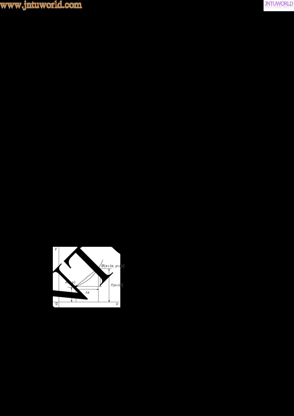
  325. 320 ENGINEERING MATHEMATICS The middle term is the seventh member,

    i.e. 4, thus the median value is 4. The modal value is the value of the most com- monly occurring member and is 3, which occurs three times, all other members only occurring once or twice. Problem 2. The following set of data refers to the amount of money in £s taken by a news vendor for 6 days. Determine the mean, median and modal values of the set: f27.90, 34.70, 54.40, 18.92, 47.60, 39.68g Mean value D 27.90 C 34.70 C 54.40 C18.92 C 47.60 C 39.68 6 D £37.20 The ranked set is: f18.92, 27.90, 34.70, 39.68, 47.60, 54.40g Since the set has an even number of members, the mean of the middle two members is taken to give the median value, i.e. median value D 34.70 C 39.68 2 D £37.19 Since no two members have the same value, this set has no mode. Now try the following exercise Exercise 131 Further problems on mean, median and mode for dis- crete data In Problems 1 to 4, determine the mean, median and modal values for the sets given. 1. f3, 8, 10, 7, 5, 14, 2, 9, 8g [mean 7.33, median 8, mode 8] 2. f26, 31, 21, 29, 32, 26, 25, 28g [mean 27.25, median 27, mode 26] 3. f4.72, 4.71, 4.74, 4.73, 4.72, 4.71, 4.73, 4.72g [mean 4.7225, median 4.72, mode 4.72] 4. f73.8, 126.4, 40.7, 141.7, 28.5, 237.4, 157.9g [mean 115.2, median 126.4, no mode] 37.3 Mean, median and mode for grouped data The mean value for a set of grouped data is found by determining the sum of the (frequency ð class mid-point values) and dividing by the sum of the frequencies, i.e. mean value x D f1x1 C f2x2 C Ð Ð Ð C fnxn f1 C f2 C Ð Ð Ð C fn D fx f where f is the frequency of the class having a mid- point value of x, and so on. Problem 3. The frequency distribution for the value of resistance in ohms of 48 resistors is as shown. Determine the mean value of resistance. 20.5–20.9 3, 21.0–21.4 10, 21.5–21.9 11, 22.0–22.4 13, 22.5–22.9 9, 23.0–23.4 2 The class mid-point/frequency values are: 20.7 3, 21.2 10, 21.7 11, 22.2 13, 22.7 9 and 23.2 2 For grouped data, the mean value is given by: x D fx f where f is the class frequency and x is the class mid-point value. Hence mean value, x D 3 ð 20.7 C 10 ð 21.2 C 11 ð 21.7 C 13 ð 22.2 C 9 ð 22.7 C 2 ð 23.2 48 D 1052.1 48 D 21.919 . . . i.e. the mean value is 21.9 ohms, correct to 3 significant figures. www.jntuworld.com JN TU W orld
  326. MEASURES OF CENTRAL TENDENCY AND DISPERSION 321 Histogram The mean,

    median and modal values for grouped data may be determined from a histogram. In a his- togram, frequency values are represented vertically and variable values horizontally. The mean value is given by the value of the variable corresponding to a vertical line drawn through the centroid of the his- togram. The median value is obtained by selecting a variable value such that the area of the histogram to the left of a vertical line drawn through the selected variable value is equal to the area of the histogram on the right of the line. The modal value is the vari- able value obtained by dividing the width of the highest rectangle in the histogram in proportion to the heights of the adjacent rectangles. The method of determining the mean, median and modal values from a histogram is shown in Problem 4. Problem 4. The time taken in minutes to assemble a device is measured 50 times and the results are as shown. Draw a histogram depicting this data and hence determine the mean, median and modal values of the distribution. 14.5–15.5 5, 16.5–17.5 8, 18.5–19.5 16, 20.5–21.5 12, 22.5–23.5 6, 24.5–25.5 3 The histogram is shown in Fig. 37.1. The mean value lies at the centroid of the histogram. With reference to any arbitrary axis, say YY shown at a time of 14 minutes, the position of the horizontal value of the centroid can be obtained from the relationship AM D am , where A is the area of the histogram, M is the horizontal distance of the centroid from the axis YY, a is the area of a rectangle of the histogram and m is the distance of the centroid of the rectangle from YY. The areas of the individual rectangles are shown circled on the histogram giving a total area of 100 square units. The positions, m, of the centroids of the individual rectangles are 1, 3, 5, . . . units from YY. Thus 100 M D 10 ð 1 C 16 ð 3 C 32 ð 5 C 24 ð 7 C 12 ð 9 C 6 ð 11 i.e. M D 560 100 D 5.6 units from YY Thus the position of the mean with reference to the time scale is 14 C 5.6, i.e. 19.6 minutes. The median is the value of time corresponding to a vertical line dividing the total area of the Figure 37.1 histogram into two equal parts. The total area is 100 square units, hence the vertical line must be drawn to give 50 units of area on each side. To achieve this with reference to Fig. 37.1, rectangle ABFE must be split so that 50 10 C 16 units of area lie on one side and 50 24 C 12 C 6 units of area lie on the other. This shows that the area of ABFE is split so that 24 units of area lie to the left of the line and 8 units of area lie to the right, i.e. the vertical line must pass through 19.5 minutes. Thus the median value of the distribution is 19.5 minutes. The mode is obtained by dividing the line AB, which is the height of the highest rectangle, pro- portionally to the heights of the adjacent rectangles. With reference to Fig. 37.1, this is done by joining AC and BD and drawing a vertical line through the point of intersection of these two lines. This gives the mode of the distribution and is 19.3 minutes. Now try the following exercise Exercise 132 Further problems on mean, median and mode for grou- ped data 1. The frequency distribution given below refers to the heights in centimetres of 100 people. Determine the mean value of the distribution, correct to the nearest millimetre. 150–156 5, 157–163 18, 164–170 20 171–177 27, 178–184 22, 185–191 8 [171.7 cm] www.jntuworld.com JN TU W orld
  327. 322 ENGINEERING MATHEMATICS 2. The gain of 90 similar transistors

    is measured and the results are as shown. 83.5–85.5 6, 86.5–88.5 39, 89.5–91.5 27, 92.5–94.5 15, 95.5–97.5 3 By drawing a histogram of this frequency distribution, determine the mean, median and modal values of the distribution. [mean 89.5, median 89, mode 88.2] 3. The diameters, in centimetres, of 60 holes bored in engine castings are measured and the results are as shown. Draw a histogram depicting these results and hence determine the mean, median and modal values of the distribution. 2.011–2.014 7, 2.016–2.019 16, 2.021–2.024 23, 2.026–2.029 9, 2.031–2.034 5 mean 2.02158 cm, median 2.02152 cm, mode 2.02167 cm 37.4 Standard deviation (a) Discrete data The standard deviation of a set of data gives an indication of the amount of dispersion, or the scatter, of members of the set from the measure of central tendency. Its value is the root-mean-square value of the members of the set and for discrete data is obtained as follows: (a) determine the measure of central tendency, usually the mean value, (occasionally the median or modal values are specified), (b) calculate the deviation of each member of the set from the mean, giving x1 x , x2 x , x3 x , . . . , (c) determine the squares of these deviations, i.e. x1 x 2, x2 x 2, x3 x 2, . . . , (d) find the sum of the squares of the deviations, that is x1 x 2 C x2 x 2 C x3 x 2, . . . , (e) divide by the number of members in the set, n, giving x1 x 2 C x2 x 2 C x3 x 2 C Ð Ð Ð n (f) determine the square root of (e). The standard deviation is indicated by (the Greek letter small ‘sigma’) and is written mathematically as: standard deviation, s = .x − x/2 n where x is a member of the set, x is the mean value of the set and n is the number of members in the set. The value of standard deviation gives an indication of the distance of the members of a set from the mean value. The set: f1, 4, 7, 10, 13g has a mean value of 7 and a standard deviation of about 4.2. The set f5, 6, 7, 8, 9g also has a mean value of 7, but the standard deviation is about 1.4. This shows that the members of the second set are mainly much closer to the mean value than the members of the first set. The method of determining the standard deviation for a set of discrete data is shown in Problem 5. Problem 5. Determine the standard deviation from the mean of the set of numbers: f5, 6, 8, 4, 10, 3g, correct to 4 significant figures. The arithmetic mean, x D x n D 5 C 6 C 8 C 4 C10 C 3 6 D 6 Standard deviation, D x x 2 n The x x 2 values are: 5 6 2, 6 6 2, 8 6 2, 4 6 2, 10 6 2 and 3 6 2. The sum of the x x 2 values, i.e. x x 2 D 1 C 0 C 4 C 4 C 16 C 9 D 34 and x x 2 n D 34 6 D 5.P 6 since there are 6 members in the set. www.jntuworld.com JN TU W orld
  328. MEASURES OF CENTRAL TENDENCY AND DISPERSION 323 Hence, standard deviation,

    s D x x2 n D 5.P 6 D 2.380 correct to 4 significant figures (b) Grouped data For grouped data, standard deviation s = ff .x − x/2g f where f is the class frequency value, x is the class mid-point value and x is the mean value of the grouped data. The method of determining the standard deviation for a set of grouped data is shown in Problem 6. Problem 6. The frequency distribution for the values of resistance in ohms of 48 resistors is as shown. Calculate the standard deviation from the mean of the resistors, correct to 3 significant figures. 20.5–20.9 3, 21.0–21.4 10, 21.5–21.9 11, 22.0–22.4 13, 22.5–22.9 9, 23.0–23.4 2 The standard deviation for grouped data is given by: D ff x x 2g f From Problem 3, the distribution mean value, x D 21.92, correct to 4 significant figures. The ‘x-values’ are the class mid-point values, i.e. 20.7, 21.2, 21.7, . . ., Thus the x x 2 values are 20.7 21.92 2, 21.2 21.92 2, 21.7 21.92 2, . . . . and the f x x 2 values are 3 20.7 21.92 2, 10 21.2 21.92 2, 11 21.7 21.92 2, . . . . The f x x 2 values are 4.4652 C 5.1840 C 0.5324 C 1.0192 C 5.4756 C 3.2768 D 19.9532 ff x x 2g f D 19.9532 48 D 0.41569 and standard deviation, s D ff x x 2g f D p 0.41569 D 0.645, correct to 3 significant figures Now try the following exercise Exercise 133 Further problems on stan- dard deviation 1. Determine the standard deviation from the mean of the set of numbers: f35, 22, 25, 23, 28, 33, 30g correct to 3 significant figures. [4.60] 2. The values of capacitances, in micro- farads, of ten capacitors selected at random from a large batch of similar capacitors are: 34.3, 25.0, 30.4, 34.6, 29.6, 28.7, 33.4, 32.7, 29.0 and 31.3 Determine the standard deviation from the mean for these capacitors, correct to 3 significant figures. [2.83 µF] 3. The tensile strength in megapascals for 15 samples of tin were determined and found to be: 34.61, 34.57, 34.40, 34.63, 34.63, 34.51, 34.49, 34.61, 34.52, 34.55, 34.58, 34.53, 34.44, 34.48 and 34.40 Calculate the mean and standard deviation from the mean for these 15 values, correct to 4 significant figures. mean 34.53 MPa, standard deviation 0.07474 MPa 4. Determine the standard deviation from the mean, correct to 4 significant figures, for www.jntuworld.com JN TU W orld
  329. 324 ENGINEERING MATHEMATICS the heights of the 100 people given

    in Problem 1 of Exercise 132, page 321. [9.394 cm] 5. Calculate the standard deviation from the mean for the data given in Problem 3 of Exercise 132, page 322, correct to 3 decimal places. [2.828] 37.5 Quartiles, deciles and percentiles Other measures of dispersion, which are sometimes used, are the quartile, decile and percentile values. The quartile values of a set of discrete data are obtained by selecting the values of members that divide the set into four equal parts. Thus for the set: f2, 3, 4, 5, 5, 7, 9, 11, 13, 14, 17g there are 11 members and the values of the members dividing the set into four equal parts are 4, 7, and 13. These values are signified by Q1, Q2 and Q3 and called the first, second and third quartile values, respectively. It can be seen that the second quartile value, Q2, is the value of the middle member and hence is the median value of the set. For grouped data the ogive may be used to deter- mine the quartile values. In this case, points are selected on the vertical cumulative frequency val- ues of the ogive, such that they divide the total value of cumulative frequency into four equal parts. Hor- izontal lines are drawn from these values to cut the ogive. The values of the variable corresponding to these cutting points on the ogive give the quartile values (see Problem 7). When a set contains a large number of members, the set can be split into ten parts, each containing an equal number of members. These ten parts are then called deciles. For sets containing a very large number of members, the set may be split into one hundred parts, each containing an equal number of members. One of these parts is called a percentile. Problem 7. The frequency distribution given below refers to the overtime worked by a group of craftsmen during each of 48 working weeks in a year. 25–29 5, 30–34 4, 35–39 7, 40–44 11, 45–49 12, 50–54 8, 55–59 1 Draw an ogive for this data and hence determine the quartile values. The cumulative frequency distribution (i.e. upper class boundary/cumulative frequency values) is: 29.5 5, 34.5 9, 39.5 16, 44.5 27, 49.5 39, 54.5 47, 59.5 48 The ogive is formed by plotting these values on a graph, as shown in Fig. 37.2. The total frequency is divided into four equal parts, each having a range of 48/4, i.e. 12. This gives cumulative frequency val- ues of 0 to 12 corresponding to the first quartile, 12 to 24 corresponding to the second quartile, 24 to 36 corresponding to the third quartile and 36 to 48 cor- responding to the fourth quartile of the distribution, i.e. the distribution is divided into four equal parts. The quartile values are those of the variable corre- sponding to cumulative frequency values of 12, 24 and 36, marked Q1, Q2 and Q3 in Fig. 37.2. These values, correct to the nearest hour, are 37 hours, 43 hours and 48 hours, respectively. The Q2 value is also equal to the median value of the distribution. One measure of the dispersion of a distribution is called the semi-interquartile range and is given by: Q3 Q1 /2, and is 48 37 /2 in this case, i.e. 51 2 hours. Figure 37.2 Problem 8. Determine the numbers contained in the (a) 41st to 50th percentile group, and (b) 8th decile group of the set of numbers shown below: 14 22 17 21 30 28 37 7 23 32 24 17 20 22 27 19 26 21 15 29 www.jntuworld.com JN TU W orld
  330. MEASURES OF CENTRAL TENDENCY AND DISPERSION 325 The set is

    ranked, giving: 7 14 15 17 17 19 20 21 21 22 22 23 24 26 27 28 29 30 32 37 (a) There are 20 numbers in the set, hence the first 10% will be the two numbers 7 and 14, the second 10% will be 15 and 17, and so on. Thus the 41st to 50th percentile group will be the numbers 21 and 22 (b) The first decile group is obtained by splitting the ranked set into 10 equal groups and select- ing the first group, i.e. the numbers 7 and 14. The second decile group are the numbers 15 and 17, and so on. Thus the 8th decile group contains the numbers 27 and 28 Now try the following exercise Exercise 134 Further problems on quar- tiles, deciles and percentiles 1. The number of working days lost due to accidents for each of 12 one-monthly periods are as shown. Determine the median and first and third quartile values for this data. 27 37 40 28 23 30 35 24 30 32 31 28 [30, 27.5, 33.5 days] 2. The number of faults occurring on a pro- duction line in a nine-week period are as shown below. Determine the median and quartile values for the data. 30 27 25 24 27 37 31 27 35 [27, 26, 33 faults] 3. Determine the quartile values and semi- interquartile range for the frequency dis- tribution given in Problem 1 of Exer- cise 132, page 321. Q1 D 164.5 cm, Q2 D 172.5 cm, Q3 D 179 cm, 7.25 cm 4. Determine the numbers contained in the 5th decile group and in the 61st to 70th percentile groups for the set of numbers: 40 46 28 32 37 42 50 31 48 45 32 38 27 33 40 35 25 42 38 41 [37 and 38; 40 and 41] 5. Determine the numbers in the 6th decile group and in the 81st to 90th percentile group for the set of numbers: 43 47 30 25 15 51 17 21 37 33 44 56 40 49 22 36 44 33 17 35 58 51 35 44 40 31 41 55 50 16 [40, 40, 41; 50, 51, 51] www.jntuworld.com JN TU W orld
  331. 38 Probability 38.1 Introduction to probability The probability of something

    happening is the like- lihood or chance of it happening. Values of proba- bility lie between 0 and 1, where 0 represents an absolute impossibility and 1 represents an absolute certainty. The probability of an event happening usually lies somewhere between these two extreme values and is expressed either as a proper or decimal fraction. Examples of probability are: that a length of copper wire has zero resistance at 100 °C 0 that a fair, six-sided dice will stop with a 3 upwards 1 6 or 0.1667 that a fair coin will land with a head upwards 1 2 or 0.5 that a length of copper wire has some resistance at 100 °C 1 If p is the probability of an event happening and q is the probability of the same event not happening, then the total probability is p C q and is equal to unity, since it is an absolute certainty that the event either does or does not occur, i.e. p Y q = 1 Expectation The expectation, E, of an event happening is defined in general terms as the product of the prob- ability p of an event happening and the number of attempts made, n, i.e. E = pn. Thus, since the probability of obtaining a 3 upwards when rolling a fair dice is 1 6 , the expec- tation of getting a 3 upwards on four throws of the dice is 1 6 ð 4, i.e. 2 3 Thus expectation is the average occurrence of an event. Dependent event A dependent event is one in which the probabil- ity of an event happening affects the probability of another ever happening. Let 5 transistors be taken at random from a batch of 100 transistors for test purposes, and the probability of there being a defec- tive transistor, p1, be determined. At some later time, let another 5 transistors be taken at random from the 95 remaining transistors in the batch and the probability of there being a defective transistor, p2, be determined. The value of p2 is different from p1 since batch size has effectively altered from 100 to 95, i.e. probability p2 is dependent on probabil- ity p1. Since transistors are drawn, and then another 5 transistors drawn without replacing the first 5, the second random selection is said to be without replacement. Independent event An independent event is one in which the probability of an event happening does not affect the probability of another event happening. If 5 transistors are taken at random from a batch of transistors and the probability of a defective transistor p1 is determined and the process is repeated after the original 5 have been replaced in the batch to give p2, then p1 is equal to p2. Since the 5 transistors are replaced between draws, the second selection is said to be with replacement. Conditional probability Conditional probability is concerned with the prob- ability of say event B occurring, given that event A has already taken place. If A and B are indepen- dent events, then the fact that event A has already occurred will not affect the probability of event B. If A and B are dependent events, then event A having occurred will effect the probability of event B. 38.2 Laws of probability The addition law of probability The addition law of probability is recognized by the word ‘or’ joining the probabilities. If pA is the probability of event A happening and pB is the probability of event B happening, the probability of event A or event B happening is given by pA C pB (provided events A and B are mutually exclusive, www.jntuworld.com JN TU W orld
  332. PROBABILITY 327 i.e. A and B are events which cannot

    occur together). Similarly, the probability of events A or B or C or . . . N happening is given by pA Y pB C pC Y · · · Y pN The multiplication law of probability The multiplication law of probability is recognized by the word ‘and’ joining the probabilities. If pA is the probability of event A happening and pB is the probability of event B happening, the probability of event A and event B happening is given by pA ðpB. Similarly, the probability of events A and B and C and . . . N happening is given by: pA × pB ð pC × · · · × pN 38.3 Worked problems on probability Problem 1. Determine the probabilities of selecting at random (a) a man, and (b) a woman from a crowd containing 20 men and 33 women. (a) The probability of selecting at random a man, p, is given by the ratio number of men number in crowd i.e. p D 20 20 C 33 D 20 53 or 0.3774 (b) The probability of selecting at random a wo- men, q, is given by the ratio number of women number in crowd i.e. q D 33 20 C 33 D 33 53 or 0.6226 (Check: the total probability should be equal to 1; p D 20 53 and q D 33 53 , thus the total probability, p C q D 20 53 C 33 53 D 1 hence no obvious error has been made). Problem 2. Find the expectation of obtain- ing a 4 upwards with 3 throws of a fair dice. Expectation is the average occurrence of an event and is defined as the probability times the number of attempts. The probability, p, of obtaining a 4 upwards for one throw of the dice, is 1 6 . Also, 3 attempts are made, hence n D 3 and the expectation, E, is pn, i.e. E D 1 6 ð 3 D 1 2 or 0.50 Problem 3. Calculate the probabilities of selecting at random: (a) the winning horse in a race in which 10 horses are running, (b) the winning horses in both the first and second races if there are 10 horses in each race. (a) Since only one of the ten horses can win, the probability of selecting at random the winning horse is number of winners number of horses , i.e. 1 10 or 0.10 (b) The probability of selecting the winning horse in the first race is 1 10 . The probability of selecting the winning horse in the second race is 1 10 . The probability of selecting the winning horses in the first and second race is given by the multiplication law of probability, i.e. probability = 1 10 ð 1 10 = 1 100 or 0.01 Problem 4. The probability of a component failing in one year due to excessive temperature is 1 20 , due to excessive vibration is 1 25 and due to excessive humidity is 1 50 . Determine the probabilities that during a one-year period a component: (a) fails due to excessive temperature and excessive vibration, (b) fails due to excessive vibration or excessive humidity, and (c) will not fail because of both excessive temperature and excessive humidity. www.jntuworld.com JN TU W orld
  333. 328 ENGINEERING MATHEMATICS Let pA be the probability of failure

    due to excessive temperature, then pA D 1 20 and pA D 19 20 (where pA is the probability of not failing.) Let pB be the probability of failure due to excessive vibration, then pB D 1 25 and pB D 24 25 Let pC be the probability of failure due to excessive humidity, then pC D 1 50 and pC D 49 50 (a) The probability of a component failing due to excessive temperature and excessive vibration is given by: pA ð pB D 1 20 ð 1 25 D 1 500 or 0.002 (b) The probability of a component failing due to excessive vibration or excessive humidity is: pB C pC D 1 25 C 1 50 D 3 50 or 0.06 (c) The probability that a component will not fail due excessive temperature and will not fail due to excess humidity is: pA ð pC D 19 20 ð 49 50 D 931 1000 or 0.931 Problem 5. A batch of 100 capacitors contains 73 that are within the required tolerance values, 17 which are below the required tolerance values, and the remainder are above the required tolerance values. Determine the probabilities that when randomly selecting a capacitor and then a second capacitor: (a) both are within the required tolerance values when selecting with replacement, and (b) the first one drawn is below and the second one drawn is above the required tolerance value, when selection is without replacement. (a) The probability of selecting a capacitor within the required tolerance values is 73 100 . The first capacitor drawn is now replaced and a second one is drawn from the batch of 100. The probability of this capacitor being within the required tolerance values is also 73 100 . Thus, the probability of selecting a capacitor within the required tolerance values for both the first and the second draw is: 73 100 ð 73 100 D 5329 10 000 or 0.5329 (b) The probability of obtaining a capacitor below the required tolerance values on the first draw is 17 100 . There are now only 99 capacitors left in the batch, since the first capacitor is not replaced. The probability of drawing a capacitor above the required tolerance values on the second draw is 10 99 , since there are 100 73 17 , i.e. 10 capacitors above the required tolerance value. Thus, the probabil- ity of randomly selecting a capacitor below the required tolerance values and followed by randomly selecting a capacitor above the tol- erance, values is 17 100 ð 10 99 D 170 9900 D 17 990 or 0.0172 Now try the following exercise Exercise 135 Further problems on proba- bility 1. In a batch of 45 lamps there are 10 faulty lamps. If one lamp is drawn at random, find the probability of it being (a) faulty and (b) satisfactory.    (a) 2 9 or 0.2222 (b) 7 9 or 0.7778    2. A box of fuses are all of the same shape and size and comprises 23 2 A fuses, 47 5 A fuses and 69 13 A fuses. Deter- mine the probability of selecting at ran- dom (a) a 2 A fuse, (b) a 5 A fuse and (c) a 13 A fuse.        (a) 23 139 or 0.1655 (b) 47 139 or 0.3381 (c) 69 139 or 0.4964        www.jntuworld.com JN TU W orld
  334. PROBABILITY 329 3. (a) Find the probability of having a

    2 upwards when throwing a fair 6-sided dice. (b) Find the probability of having a 5 upwards when throwing a fair 6- sided dice. (c) Determine the probability of having a 2 and then a 5 on two succes- sive throws of a fair 6-sided dice. (a) 1 6 (b) 1 6 (c) 1 36 4. The probability of event A happening is 3 5 and the probability of event B hap- pening is 2 3 . Calculate the probabilities of (a) both A and B happening, (b) only event A happening, i.e. event A happen- ing and event B not happening, (c) only event B happening, and (d) either A, or B, or A and B happening. (a) 2 5 (b) 1 5 (c) 4 15 (d) 13 15 5. When testing 1000 soldered joints, 4 fai- led during a vibration test and 5 failed due to having a high resistance. Deter- mine the probability of a joint failing due to (a) vibration, (b) high resistance, (c) vibration or high resistance and (d) vi- bration and high resistance.    (a) 1 250 (b) 1 200 (c) 9 1000 (d) 1 50000    38.4 Further worked problems on probability Problem 6. A batch of 40 components contains 5 which are defective. A component is drawn at random from the batch and tested and then a second component is drawn. Determine the probability that neither of the components is defective when drawn (a) with replacement, and (b) without replacement. (a) With replacement The probability that the component selected on the first draw is satisfactory is 35 40 , i.e. 7 8 . The component is now replaced and a second draw is made. The probability that this component is also satisfactory is 7 8 . Hence, the probability that both the first component drawn and the second compo- nent drawn are satisfactory is: 7 8 ð 7 8 D 49 64 or 0.7656 (b) Without replacement The probability that the first component drawn is sat- isfactory is 7 8 . There are now only 34 satisfactory components left in the batch and the batch number is 39. Hence, the probability of drawing a satisfac- tory component on the second draw is 34 39 . Thus the probability that the first component drawn and the second component drawn are satisfactory, i.e. neither is defective, is: 7 8 ð 34 39 D 238 312 or 0.7628 Problem 7. A batch of 40 components contains 5 that are defective. If a component is drawn at random from the batch and tested and then a second component is drawn at random, calculate the probability of having one defective component, both with and without replacement. The probability of having one defective component can be achieved in two ways. If p is the proba- bility of drawing a defective component and q is the probability of drawing a satisfactory component, then the probability of having one defective compo- nent is given by drawing a satisfactory component and then a defective component or by drawing a defective component and then a satisfactory one, i.e. by q ð p C p ð q With replacement: p D 5 40 D 1 8 and q D 35 40 D 7 8 Hence, probability of having one defective compo- nent is: 1 8 ð 7 8 C 7 8 ð 1 8 www.jntuworld.com JN TU W orld
  335. 330 ENGINEERING MATHEMATICS i.e. 7 64 C 7 64 D

    7 32 or 0.2188 Without replacement: p1 D 1 8 and q1 D 7 8 on the first of the two draws. The batch number is now 39 for the second draw, thus, p2 D 5 39 and q2 D 35 39 p1q2 C q1p2 D 1 8 ð 35 39 C 7 8 ð 5 39 D 35 C 35 312 D 70 312 or 0.2244 Problem 8. A box contains 74 brass washers, 86 steel washers and 40 aluminium washers. Three washers are drawn at random from the box without replacement. Determine the probability that all three are steel washers. Assume, for clarity of explanation, that a washer is drawn at random, then a second, then a third (although this assumption does not affect the results obtained). The total number of washers is 74C86C 40, i.e. 200. The probability of randomly selecting a steel washer on the first draw is 86 200 . There are now 85 steel washers in a batch of 199. The probability of randomly selecting a steel washer on the second draw is 85 199 . There are now 84 steel washers in a batch of 198. The probability of randomly selecting a steel washer on the third draw is 84 198 . Hence the probability of selecting a steel washer on the first draw and the second draw and the third draw is: 86 200 ð 85 199 ð 84 198 D 614 040 7 880 400 D 0.0779 Problem 9. For the box of washers given in Problem 8 above, determine the probability that there are no aluminium washers drawn, when three washers are drawn at random from the box without replacement. The probability of not drawing an aluminium washer on the first draw is 1 40 200 , i.e. 160 200 . There are now 199 washers in the batch of which 159 are not aluminium washers. Hence, the probability of not drawing an aluminium washer on the second draw is 159 199 . Similarly, the probability of not drawing an aluminium washer on the third draw is 158 198 . Hence the probability of not drawing an aluminium washer on the first and second and third draws is 160 200 ð 159 199 ð 158 198 D 4 019 520 7 880 400 D 0.5101 Problem 10. For the box of washers in Problem 8 above, find the probability that there are two brass washers and either a steel or an aluminium washer when three are drawn at random, without replacement. Two brass washers (A) and one steel washer (B) can be obtained in any of the following ways: 1st draw 2nd draw 3rd draw A A B A B A B A A Two brass washers and one aluminium washer (C) can also be obtained in any of the following ways: 1st draw 2nd draw 3rd draw A A C A C A C A A Thus there are six possible ways of achieving the combinations specified. If A represents a brass washer, B a steel washer and C an aluminium washer, then the combinations and their probabilities are as shown: www.jntuworld.com JN TU W orld
  336. PROBABILITY 331 Draw Probability First Second Third A A B

    74 200 ð 73 199 ð 86 198 D 0.0590 A B A 74 200 ð 86 199 ð 73 198 D 0.0590 B A A 86 200 ð 74 199 ð 73 198 D 0.0590 A A C 74 200 ð 73 199 ð 40 198 D 0.0274 A C A 74 200 ð 40 199 ð 73 198 D 0.0274 C A A 40 200 ð 74 199 ð 73 198 D 0.0274 The probability of having the first combination or the second, or the third, and so on, is given by the sum of the probabilities, i.e. by 3 ð 0.0590 C 3 ð 0.0274, that is, 0.2592 Now try the following exercise Exercise 136 Further problems on proba- bility 1. The probability that component A will operate satisfactorily for 5 years is 0.8 and that B will operate satisfactorily over that same period of time is 0.75. Find the probabilities that in a 5 year period: (a) both components operate satisfacto- rily, (b) only component A will operate satisfactorily, and (c) only component B will operate satisfactorily. [(a) 0.6 (b) 0.2 (c) 0.15] 2. In a particular street, 80% of the houses have telephones. If two houses selected at random are visited, calculate the probabil- ities that (a) they both have a telephone and (b) one has a telephone but the other does not have telephone. [(a) 0.64 (b) 0.32] 3. Veroboard pins are packed in packets of 20 by a machine. In a thousand pack- ets, 40 have less than 20 pins. Find the probability that if 2 packets are chosen at random, one will contain less than 20 pins and the other will contain 20 pins or more. [0.0768] 4. A batch of 1 kW fire elements contains 16 which are within a power tolerance and 4 which are not. If 3 elements are selected at random from the batch, calcu- late the probabilities that (a) all three are within the power tolerance and (b) two are within but one is not within the power tolerance. [(a) 0.4912 (b) 0.4211] 5. An amplifier is made up of three transis- tors, A, B and C. The probabilities of A, B or C being defective are 1 20 , 1 25 and 1 50 , respectively. Calculate the percentage of amplifiers produced (a) which work sat- isfactorily and (b) which have just one defective transistor. [(a) 89.38% (b) 10.25%] 6. A box contains 14 40 W lamps, 28 60 W lamps and 58 25 W lamps, all the lamps being of the same shape and size. Three lamps are drawn at random from the box, first one, then a second, then a third. Determine the probabilities of: (a) getting one 25 W, one 40 W and one 60 W lamp, with replacement, (b) getting one 25 W, one 40 W and one 60 W lamp without replacement, and (c) getting either one 25 W and two 40 W or one 60 W and two 40 W lamps with replacement. [(a) 0.0227 (b) 0.0234 (c) 0.0169] 38.5 Permutations and combinations Permutations If n different objects are available, they can be arranged in different orders of selection. Each dif- ferent ordered arrangement is called a permutation. For example, permutations of the three letters X, Y and Z taken together are: XYZ, XZY, YXZ, YZX, ZXY and ZYX This can be expressed as 3P3 D 6, the upper 3 denoting the number of items from which the arrangements are made, and the lower 3 indicating the number of items used in each arrangement. If we take the same three letters XYZ two at a time the permutations XY, YZ, XZ, ZX, YZ, ZY can be found, and denoted by 3P2 D 6 www.jntuworld.com JN TU W orld
  337. 332 ENGINEERING MATHEMATICS (Note that the order of the letters

    matter in permu- tations, i.e. YX is a different permutation from XY). In general, nPr D n n 1 n 2 . . . n r C 1 or n Pr = n! .n − r/! as stated in Chapter 14 For example, 5P4 D 5 4 3 2 D 120 or 5P4 D 5! 5 4 ! D 5! 1! D 5 4 3 2 D 120 Also, 3P3 D 6 from above; using nPr D n! n r ! gives 3P3 D 3! 3 3 ! D 6 0! . Since this must equal 6, then 0! = 1 (check this with your calculator). Combinations If selections of the three letters X, Y, Z are made without regard to the order of the letters in each group, i.e. XY is now the same as YX for exam- ple, then each group is called a combination. The number of possible combinations is denoted by nCr, where n is the total number of items and r is the number in each selection. In general, nCr D n! r!.n − r/! For example, 5C4 D 5! 4! 5 4 ! D 5! 4! D 5 ð 4 ð 3 ð 2 ð 1 4 ð 3 ð 2 ð 1 D 5 Problem 11. Calculate the number of permutations there are of: (a) 5 distinct objects taken 2 at a time, (b) 4 distinct objects taken 2 at a time. (a) 5P2 D 5! 5 2 ! D 5! 3! D 5 ð 4 ð 3 ð 2 3 ð 2 D 20 (b) 4P2 D 4! 4 2 ! D 4! 2! D 12 Problem 12. Calculate the number of combinations there are of: (a) 5 distinct objects taken 2 at a time, (b) 4 distinct objects taken 2 at a time. (a) 5C2 D 5! 2! 5 2 ! D 5! 2! 3! D 5 ð 4 ð 3 ð 2 ð 1 2 ð 1 3 ð 2 ð 1 D 10 (b) 4C2 D 4! 2! 4 2 ! D 4! 2! 2! D 6 Problem 13. A class has 24 students. 4 can represent the class at an exam board. How many combinations are possible when choosing this group. Number of combinations possible, nCr D n! r! n r ! i.e. 24C4 D 24! 4! 24 4 ! D 24! 4! 20! = 10 626 Problem 14. In how many ways can a team of eleven be picked from sixteen possible players? Number of ways D nCr D 16C11 D 16! 11! 16 11 ! D 16! 11! 5! D 4368 Now try the following exercise Exercise 137 Further problems on per- mutations and combinations 1. Calculate the number of permutations there are of: (a) 15 distinct objects taken 2 at a time, (b) 9 distinct objects taken 4 at a time. [(a) 210 (b) 3024] 2. Calculate the number of combinations there are of: (a) 12 distinct objects taken 5 at a time, (b) 6 distinct objects taken 4 at a time. [(a) 792 (b) 15] 3. In how many ways can a team of six be picked from ten possible players? [210] 4. 15 boxes can each hold one object. In how many ways can 10 identical objects be placed in the boxes? [3003] www.jntuworld.com JN TU W orld
  338. 39 The binomial and Poisson distribution 39.1 The binomial distribution

    The binomial distribution deals with two numbers only, these being the probability that an event will happen, p, and the probability that an event will not happen, q. Thus, when a coin is tossed, if p is the probability of the coin landing with a head upwards, q is the probability of the coin landing with a tail upwards. p C q must always be equal to unity. A binomial distribution can be used for finding, say, the probability of getting three heads in seven tosses of the coin, or in industry for determining defect rates as a result of sampling. One way of defining a binomial distribution is as follows: ‘if p is the probability that an event will happen and q is the probability that the event will not happen, then the probabilities that the event will happen 0, 1, 2, 3, . . ., n times in n trials are given by the successive terms of the expansion of q C p n taken from left to right’. The binomial expansion of q C p n is: qn C nqn 1p C n n 1 2! qn 2p2 C n n 1 n 2 3! qn 3p3 C Ð Ð Ð from Chapter 15 This concept of a binomial distribution is used in Problems 1 and 2. Problem 1. Determine the probabilities of having (a) at least 1 girl and (b) at least 1 girl and 1 boy in a family of 4 children, assuming equal probability of male and female birth The probability of a girl being born, p, is 0.5 and the probability of a girl not being born (male birth), q, is also 0.5. The number in the family, n, is 4. From above, the probabilities of 0, 1, 2, 3, 4 girls in a family of 4 are given by the successive terms of the expansion of q C p 4 taken from left to right. From the binomial expansion: q C p 4 D q4 C 4q3p C 6q2p2 C 4qp3 C p4 Hence the probability of no girls is q4, i.e. 0.54 D 0.0625 the probability of 1 girl is 4q3p, i.e. 4 ð 0.53 ð 0.5 D 0.2500 the probability of 2 girls is 6q2p2, i.e. 6 ð 0.52 ð 0.52 D 0.3750 the probability of 3 girls is 4qp3, i.e. 4 ð 0.5 ð 0.53 D 0.2500 the probability of 4 girls is p4, i.e. 0.54 D 0.0625 Total probability, q C p 4 D 1.0000 (a) The probability of having at least one girl is the sum of the probabilities of having 1, 2, 3 and 4 girls, i.e. 0.2500 C 0.3750 C 0.2500 C 0.0625 D 0.9375 (Alternatively, the probability of having at least 1 girl is: 1 (the probability of having no girls), i.e. 1 0.0625, giving 0.9375, as obtained previously). (b) The probability of having at least 1 girl and 1 boy is given by the sum of the probabilities of having: 1 girl and 3 boys, 2 girls and 2 boys and 3 girls and 2 boys, i.e. 0.2500 C 0.3750 C 0.2500 D 0.8750 (Alternatively, this is also the probability of having 1 (probability of having no girls C probability of having no boys), i.e. 1 2 ð 0.0625 D 0.8750, as obtained previ- ously). www.jntuworld.com JN TU W orld
  339. 334 ENGINEERING MATHEMATICS Problem 2. A dice is rolled 9

    times. Find the probabilities of having a 4 upwards (a) 3 times and (b) less than 4 times Let p be the probability of having a 4 upwards. Then p D 1/6, since dice have six sides. Let q be the probability of not having a 4 upwards. Then q D 5/6. The probabilities of having a 4 upwards 0, 1, 2 . . . n times are given by the suc- cessive terms of the expansion of q C p n, taken from left to right. From the binomial expansion: q C q 9 D q9 C 9q8p C 36q7p2 C 84q6p3 C Ð Ð Ð The probability of having a 4 upwards no times is q9 D 5/6 9 D 0.1938 The probability of having a 4 upwards once is 9q8p D 9 5/6 8 1/6 D 0.3489 The probability of having a 4 upwards twice is 36q7p2 D 36 5/6 7 1/6 2 D 0.2791 The probability of having a 4 upwards 3 times is 84q6p3 D 84 5/6 6 1/6 3 D 0.1302 (a) The probability of having a 4 upwards 3 times is 0.1302 (b) The probability of having a 4 upwards less than 4 times is the sum of the probabilities of having a 4 upwards 0, 1, 2, and 3 times, i.e. 0.1938 C 0.3489 C 0.2791 C 0.1302 D 0.9520 Industrial inspection In industrial inspection, p is often taken as the probability that a component is defective and q is the probability that the component is satisfactory. In this case, a binomial distribution may be defined as: ‘the probabilities that 0, 1, 2, 3, . . ., n components are defective in a sample of n components, drawn at random from a large batch of components, are given by the successive terms of the expansion of q C p n, taken from left to right’. This definition is used in Problems 3 and 4. Problem 3. A machine is producing a large number of bolts automatically. In a box of these bolts. 95% are within the allowable tolerance values with respect to diameter, the remainder being outside of the diameter tolerance values. Seven bolts are drawn at random from the box. Determine the probabilities that (a) two and (b) more than two of the seven bolts are outside of the diameter tolerance values Let p be the probability that a bolt is outside of the allowable tolerance values, i.e. is defective, and let q be the probability that a bolt is within the tolerance values, i.e. is satisfactory. Then p D 5%, i.e. 0.05 per unit and q D 95%, i.e. 0.95 per unit. The sample number is 7. The probabilities of drawing 0, 1, 2, . . ., n defec- tive bolts are given by the successive terms of the expansion of q C p n, taken from left to right. In this problem q C p n D 0.95 C 0.05 7 D 0.957 C 7 ð 0.956 ð 0.05 C 21 ð 0.955 ð 0.052 C Ð Ð Ð Thus the probability of no defective bolts is: 0.957 D 0.6983 The probability of 1 defective bolt is: 7 ð 0.956 ð 0.05 D 0.2573 The probability of 2 defective bolts is: 21 ð 0.955 ð 0.052 D 0.0406, and so on. (a) The probability that two bolts are outside of the diameter tolerance values is 0.0406 (b) To determine the probability that more than two bolts are defective, the sum of the proba- bilities of 3 bolts, 4 bolts, 5 bolts, 6 bolts and 7 bolts being defective can be determined. An easier way to find this sum is to find 1 (sum of 0 bolts, 1 bolt and 2 bolts being defective), since the sum of all the terms is unity. Thus, the probability of there being more than two bolts outside of the tolerance values is: 1 0.6983 C 0.2573 C 0.0406 , i.e. 0.0038 Problem 4. A package contains 50 similar components and inspection shows that four have been damaged during transit. If six components are drawn at random from the www.jntuworld.com JN TU W orld
  340. THE BINOMIAL AND POISSON DISTRIBUTION 335 contents of the package

    determine the probabilities that in this sample (a) one and (b) less than three are damaged The probability of a component being damaged, p, is 4 in 50, i.e. 0.08 per unit. Thus, the probability of a component not being damaged, q, is 1 0.08, i.e. 0.92 The probability of there being 0, 1, 2, . . ., 6 damaged components is given by the successive terms of q C p 6, taken from left to right. q C p 6 D q6 C 6q5p C 15q4p2 C 20q3p3 C Ð Ð Ð (a) The probability of one damaged component is 6q5p D 6 ð 0.925 ð 0.08 D 0.3164 (b) The probability of less than three damaged components is given by the sum of the proba- bilities of 0, 1 and 2 damaged components. q6 C 6q5p C 15q4p2 D 0.926 C 6 ð 0.925 ð 0.08 C 15 ð 0.924 ð 0.082 D 0.6064 C 0.3164 C 0.0688 D 0.9916 Histogram of probabilities The terms of a binomial distribution may be repre- sented pictorially by drawing a histogram, as shown in Problem 5. Problem 5. The probability of a student successfully completing a course of study in three years is 0.45. Draw a histogram showing the probabilities of 0, 1, 2, . . ., 10 students successfully completing the course in three years Let p be the probability of a student successfully completing a course of study in three years and q be the probability of not doing so. Then p D 0.45 and q D 0.55. The number of students, n, is 10. The probabilities of 0, 1, 2, . . ., 10 students suc- cessfully completing the course are given by the successive terms of the expansion of qCp 10, taken from left to right. q C p 10 D q10 C 10q9p C 45q8p2 C 120q7p3 C 210q6p4 C 252q5p5 C 210q4p6 C 120q3p7 C 45q2p8 C 10qp9 C p10 0 1 2 3 4 5 6 7 8 9 10 0.02 0.04 0.06 0.08 0.10 0.12 0.14 0.16 0.18 0.20 0.22 0.24 Probability of successfully completing course Number of students 0 Figure 39.1 Substituting q D 0.55 and p D 0.45 in this expan- sion gives the values of the successive terms as: 0.0025, 0.0207, 0.0763, 0.1665, 0.2384, 0.2340, 0.1596, 0.0746, 0.0229, 0.0042 and 0.0003. The histogram depicting these probabilities is shown in Fig. 39.1. Now try the following exercise Exercise 138 Further problems on the binomial distribution 1. Concrete blocks are tested and it is found that, on average, 7% fail to meet the required specification. For a batch of 9 blocks, determine the probabilities that (a) three blocks and (b) less than four blocks will fail to meet the specification. [(a) 0.0186 (b) 0.9976] 2. If the failure rate of the blocks in Prob- lem 1 rises to 15%, find the probabilities www.jntuworld.com JN TU W orld
  341. 336 ENGINEERING MATHEMATICS that (a) no blocks and (b) more

    than two blocks will fail to meet the specification in a batch of 9 blocks. [(a) 0.2316 (b) 0.1408] 3. The average number of employees absent from a firm each day is 4%. An office within the firm has seven employees. Determine the probabilities that (a) no employee and (b) three employees will be absent on a particular day. [(a) 0.7514 (b) 0.0019] 4. A manufacturer estimates that 3% of his output of a small item is defective. Find the probabilities that in a sample of 10 items (a) less than two and (b) more than two items will be defective. [(a) 0.9655 (b) 0.0028] 5. Five coins are tossed simultaneously. Determine the probabilities of having 0, 1, 2, 3, 4 and 5 heads upwards, and draw a histogram depicting the results.      Vertical adjacent rectangles, whose heights are proportional to 0.0313, 0.1563, 0.3125, 0.3125, 0.1563 and 0.0313      6. If the probability of rain falling during a particular period is 2/5, find the probabilities of having 0, 1, 2, 3, 4, 5, 6 and 7 wet days in a week. Show these results on a histogram.        Vertical adjacent rectangles, whose heights are proportional to 0.0280, 0.1306, 0.2613, 0.2903, 0.1935, 0.0774, 0.0172 and 0.0016        7. An automatic machine produces, on aver- age, 10% of its components outside of the tolerance required. In a sample of 10 components from this machine, determine the probability of having three compo- nents outside of the tolerance required by assuming a binomial distribution. [0.0574] 39.2 The Poisson distribution When the number of trials, n, in a binomial distri- bution becomes large (usually taken as larger than 10), the calculations associated with determining the values of the terms become laborious. If n is large and p is small, and the product np is less than 5, a very good approximation to a binomial distribution is given by the corresponding Poisson distribution, in which calculations are usually simpler. The Poisson approximation to a binomial distri- bution may be defined as follows: ‘the probabilities that an event will happen 0, 1, 2, 3, . . ., n times in n trials are given by the successive terms of the expression e 1 C C 2 2! C 3 3! C Ð Ð Ð taken from left to right’ The symbol is the expectation of an event hap- pening and is equal to np. Problem 6. If 3% of the gearwheels produced by a company are defective, determine the probabilities that in a sample of 80 gearwheels (a) two and (b) more than two will be defective. The sample number, n, is large, the probability of a defective gearwheel, p, is small and the product np is 80 ð 0.03, i.e. 2.4, which is less than 5. Hence a Poisson approximation to a binomial distribution may be used. The expectation of a defective gear- wheel, D np D 2.4 The probabilities of 0, 1, 2, . . . defective gear- wheels are given by the successive terms of the expression e 1 C C 2 2! C 3 3! C Ð Ð Ð taken from left to right, i.e. by e , e , 2e 2! , . . . Thus: probability of no defective gearwheels is e D e 2.4 D 0.0907 probability of 1 defective gearwheel is e D 2.4e 2.4 D 0.2177 www.jntuworld.com JN TU W orld
  342. THE BINOMIAL AND POISSON DISTRIBUTION 337 probability of 2 defective

    gearwheels is 2e 2! D 2.42e 2.4 2 ð 1 D 0.2613 (a) The probability of having 2 defective gear- wheels is 0.2613 (b) The probability of having more than 2 defective gearwheels is 1 (the sum of the probabilities of having 0, 1, and 2 defective gearwheels), i.e. 1 0.0907 C 0.2177 C 0.2613 , that is, 0.4303 The principal use of a Poisson distribution is to determine the theoretical probabilities when p, the probability of an event happening, is known, but q, the probability of the event not happening is unknown. For example, the average number of goals scored per match by a football team can be calcu- lated, but it is not possible to quantify the num- ber of goals that were not scored. In this type of problem, a Poisson distribution may be defined as follows: ‘the probabilities of an event occurring 0, 1, 2, 3 . . . times are given by the successive terms of the expres- sion e 1 C C 2 2! C 3 3! C Ð Ð Ð , taken from left to right’ The symbol is the value of the average occurrence of the event. Problem 7. A production department has 35 similar milling machines. The number of breakdowns on each machine averages 0.06 per week. Determine the probabilities of having (a) one, and (b) less than three machines breaking down in any week Since the average occurrence of a breakdown is known but the number of times when a machine did not break down is unknown, a Poisson distribution must be used. The expectation of a breakdown for 35 machines is 35 ð 0.06, i.e. 2.1 breakdowns per week. The probabilities of a breakdown occurring 0, 1, 2,. . . times are given by the successive terms of the expression e 1 C C 2 2! C 3 3! C Ð Ð Ð , taken from left to right. Hence: probability of no breakdowns e D e 2.1 D 0.1225 probability of 1 breakdown is e D 2.1e 2.1 D 0.2572 probability of 2 breakdowns is 2e 2! D 2.12e 2.1 2 ð 1 D 0.2700 (a) The probability of 1 breakdown per week is 0.2572 (b) The probability of less than 3 breakdowns per week is the sum of the probabilities of 0, 1 and 2 breakdowns per week, i.e. 0.1225 C 0.2572 C 0.2700 D 0.6497 Histogram of probabilities The terms of a Poisson distribution may be repre- sented pictorially by drawing a histogram, as shown in Problem 8. Problem 8. The probability of a person having an accident in a certain period of time is 0.0003. For a population of 7500 people, draw a histogram showing the probabilities of 0, 1, 2, 3, 4, 5 and 6 people having an accident in this period. The probabilities of 0, 1, 2, . . . people having an accident are given by the terms of the expression e 1 C C 2 2! C 3 3! C Ð Ð Ð , taken from left to right. The average occurrence of the event, , is 7500 ð 0.0003, i.e. 2.25 The probability of no people having an accident is e D e 2.25 D 0.1054 www.jntuworld.com JN TU W orld
  343. 338 ENGINEERING MATHEMATICS 0 1 2 3 4 5 6

    Number of people 0.04 0.08 0.12 0.16 0.20 0.24 0.28 Probability of having an accident 0 Figure 39.2 The probability of 1 person having an accident is e D 2.25e 2.25 D 0.2371 The probability of 2 people having an accident is 2e 2! D 2.252e 2.25 2! D 0.2668 and so on, giving probabilities of 0.2001, 0.1126, 0.0506 and 0.0190 for 3, 4, 5 and 6 respectively having an accident. The histogram for these proba- bilities is shown in Fig. 39.2. Now try the following exercise Exercise 139 Further problems on the Poisson distribution 1. In problem 7 of Exercise 138, page 336, determine the probability of having three components outside of the required tolerance using the Poisson distribution. [0.0613] 2. The probability that an employee will go to hospital in a certain period of time is 0.0015. Use a Poisson distribution to determine the probability of more than two employees going to hospital during this period of time if there are 2000 employees on the payroll. [0.5768] 3. When packaging a product, a manufac- turer finds that one packet in twenty is underweight. Determine the probabilities that in a box of 72 packets (a) two and (b) less than four will be underweight. [(a) 0.1771 (b) 0.5153] 4. A manufacturer estimates that 0.25% of his output of a component are defective. The components are marketed in packets of 200. Determine the probability of a packet containing less than three defective components. [0.9856] 5. The demand for a particular tool from a store is, on average, five times a day and the demand follows a Poisson distribution. How many of these tools should be kept in the stores so that the probability of there being one available when required is greater than 10%?                 The probabilities of the demand for 0, 1, 2, . . . tools are 0.0067, 0.0337, 0.0842, 0.1404, 0.1755, 0.1755, 0.1462, 0.1044, 0.0653, . . . This shows that the probability of wanting a tool 8 times a day is 0.0653, i.e. less than 10%. Hence 7 should be kept in the store                 6. Failure of a group of particular machine tools follows a Poisson distribution with a mean value of 0.7. Determine the probabilities of 0, 1, 2, 3, 4 and 5 failures in a week and present these results on a histogram.     Vertical adjacent rectangles having heights proportional to 0.4966, 0.3476, 0.1217, 0.0284, 0.0050 and 0.0007     www.jntuworld.com JN TU W orld
  344. THE BINOMIAL AND POISSON DISTRIBUTION 339 Assignment 10 This assignment

    covers the material in Chapters 36 to 39. The marks for each question are shown in brackets at the end of each question. 1. A company produces five products in the following proportions: Product A 24 Product B 16 Product C 15 Product D 11 Product E 6 Present these data visually by drawing (a) a vertical bar chart (b) a percentage bar chart (c) a pie diagram. (13) 2. The following lists the diameters of 40 components produced by a machine, each measured correct to the nearest hundredth of a centimetre: 1.39 1.36 1.38 1.31 1.33 1.40 1.28 1.40 1.24 1.28 1.42 1.34 1.43 1.35 1.36 1.36 1.35 1.45 1.29 1.39 1.38 1.38 1.35 1.42 1.30 1.26 1.37 1.33 1.37 1.34 1.34 1.32 1.33 1.30 1.38 1.41 1.35 1.38 1.27 1.37 (a) Using 8 classes form a frequency distri- bution and a cumulative frequency distri- bution. (b) For the above data draw a histogram, a frequency polygon and an ogive. (21) 3. Determine for the 10 measurements of lengths shown below: (a) the arithmetic mean, (b) the median, (c) the mode, and (d) the standard devia- tion. 28 m, 20 m, 32 m, 44 m, 28 m, 30 m, 30 m, 26 m, 28 m and 34 m (9) 4. The heights of 100 people are measured correct to the nearest centimetre with the following results: 150–157 cm 5 158–165 cm 18 166–173 cm 42 174–181 cm 27 182–189 cm 8 Determine for the data (a) the mean height and (b) the standard deviation. (10) 5. Determine the probabilities of: (a) drawing a white ball from a bag con- taining 6 black and 14 white balls (b) winning a prize in a raffle by buying 6 tickets when a total of 480 tickets are sold (c) selecting at random a female from a group of 12 boys and 28 girls (d) winning a prize in a raffle by buying 8 tickets when there are 5 prizes and a total of 800 tickets are sold. (8) 6. In a box containing 120 similar transistors 70 are satisfactory, 37 give too high a gain under normal operating conditions and the remainder give too low a gain. Calculate the probability that when draw- ing two transistors in turn, at random, with replacement, of having (a) two satisfac- tory, (b) none with low gain, (c) one with high gain and one satisfactory, (d) one with low gain and none satisfactory. Determine the probabilities in (a), (b) and (c) above if the transistors are drawn without replacement. (14) 7. A machine produces 15% defective components. In a sample of 5, drawn at random, calculate, using the binomial distribution, the probability that: (a) there will be 4 defective items (b) there will be not more than 3 defec- tive items (c) all the items will be non-defective (13) 8. 2% of the light bulbs produced by a company are defective. Determine, using the Poisson distribution, the probability that in a sample of 80 bulbs: (a) 3 bulbs will be defective, (b) not more than 3 bulbs will be defective, (c) at least 2 bulbs will be defective. (12) www.jntuworld.com JN TU W orld
  345. 40 The normal distribution 40.1 Introduction to the normal distribution

    When data is obtained, it can frequently be consid- ered to be a sample (i.e. a few members) drawn at random from a large population (i.e. a set hav- ing many members). If the sample number is large, it is theoretically possible to choose class intervals which are very small, but which still have a number of members falling within each class. A frequency polygon of this data then has a large number of small line segments and approximates to a continu- ous curve. Such a curve is called a frequency or a distribution curve. An extremely important symmetrical distribution curve is called the normal curve and is as shown in Fig. 40.1. This curve can be described by a mathematical equation and is the basis of much of the work done in more advanced statistics. Many natural occurrences such as the heights or weights of a group of people, the sizes of components produced by a particular machine and the life length of certain components approximate to a normal distribution. Variable Frequency Figure 40.1 Normal distribution curves can differ from one another in the following four ways: (a) by having different mean values (b) by having different values of standard deviations (c) the variables having different values and different units and (d) by having different areas between the curve and the horizontal axis. A normal distribution curve is standardised as follows: (a) The mean value of the unstandardised curve is made the origin, thus making the mean value, x, zero. (b) The horizontal axis is scaled in standard devia- tions. This is done by letting z D x x , where z is called the normal standard variate, x is the value of the variable, x is the mean value of the distribution and is the standard deviation of the distribution. (c) The area between the normal curve and the horizontal axis is made equal to unity. When a normal distribution curve has been stan- dardised, the normal curve is called a standardised normal curve or a normal probability curve, and any normally distributed data may be represented by the same normal probability curve. The area under part of a normal probability curve is directly proportional to probability and the value of the shaded area shown in Fig. 40.2 can be deter- mined by evaluating: 1 p 2 e z2/2 dz, where z D x x Probability density Standard deviations z1 z2 0 z-value Figure 40.2 To save repeatedly determining the values of this function, tables of partial areas under the standardised normal curve are available in many mathematical formulae books, and such a table is shown in Table 40.1. www.jntuworld.com JN TU W orld
  346. THE NORMAL DISTRIBUTION 341 Table 40.1 Partial areas under the

    standardised normal curve 0 z z D x x 0 1 2 3 4 5 6 7 8 9 0.0 0.0000 0.0040 0.0080 0.0120 0.0159 0.0199 0.0239 0.0279 0.0319 0.0359 0.1 0.0398 0.0438 0.0478 0.0517 0.0557 0.0596 0.0636 0.0678 0.0714 0.0753 0.2 0.0793 0.0832 0.0871 0.0910 0.0948 0.0987 0.1026 0.1064 0.1103 0.1141 0.3 0.1179 0.1217 0.1255 0.1293 0.1331 0.1388 0.1406 0.1443 0.1480 0.1517 0.4 0.1554 0.1591 0.1628 0.1664 0.1700 0.1736 0.1772 0.1808 0.1844 0.1879 0.5 0.1915 0.1950 0.1985 0.2019 0.2054 0.2086 0.2123 0.2157 0.2190 0.2224 0.6 0.2257 0.2291 0.2324 0.2357 0.2389 0.2422 0.2454 0.2486 0.2517 0.2549 0.7 0.2580 0.2611 0.2642 0.2673 0.2704 0.2734 0.2760 0.2794 0.2823 0.2852 0.8 0.2881 0.2910 0.2939 0.2967 0.2995 0.3023 0.3051 0.3078 0.3106 0.3133 0.9 0.3159 0.3186 0.3212 0.3238 0.3264 0.3289 0.3315 0.3340 0.3365 0.3389 1.0 0.3413 0.3438 0.3451 0.3485 0.3508 0.3531 0.3554 0.3577 0.3599 0.3621 1.1 0.3643 0.3665 0.3686 0.3708 0.3729 0.3749 0.3770 0.3790 0.3810 0.3830 1.2 0.3849 0.3869 0.3888 0.3907 0.3925 0.3944 0.3962 0.3980 0.3997 0.4015 1.3 0.4032 0.4049 0.4066 0.4082 0.4099 0.4115 0.4131 0.4147 0.4162 0.4177 1.4 0.4192 0.4207 0.4222 0.4236 0.4251 0.4265 0.4279 0.4292 0.4306 0.4319 1.5 0.4332 0.4345 0.4357 0.4370 0.4382 0.4394 0.4406 0.4418 0.4430 0.4441 1.6 0.4452 0.4463 0.4474 0.4484 0.4495 0.4505 0.4515 0.4525 0.4535 0.4545 1.7 0.4554 0.4564 0.4573 0.4582 0.4591 0.4599 0.4608 0.4616 0.4625 0.4633 1.8 0.4641 0.4649 0.4656 0.4664 0.4671 0.4678 0.4686 0.4693 0.4699 0.4706 1.9 0.4713 0.4719 0.4726 0.4732 0.4738 0.4744 0.4750 0.4756 0.4762 0.4767 2.0 0.4772 0.4778 0.4783 0.4785 0.4793 0.4798 0.4803 0.4808 0.4812 0.4817 2.1 0.4821 0.4826 0.4830 0.4834 0.4838 0.4842 0.4846 0.4850 0.4854 0.4857 2.2 0.4861 0.4864 0.4868 0.4871 0.4875 0.4878 0.4881 0.4884 0.4882 0.4890 2.3 0.4893 0.4896 0.4898 0.4901 0.4904 0.4906 0.4909 0.4911 0.4913 0.4916 2.4 0.4918 0.4920 0.4922 0.4925 0.4927 0.4929 0.4931 0.4932 0.4934 0.4936 2.5 0.4938 0.4940 0.4941 0.4943 0.4945 0.4946 0.4948 0.4949 0.4951 0.4952 2.6 0.4953 0.4955 0.4956 0.4957 0.4959 0.4960 0.4961 0.4962 0.4963 0.4964 2.7 0.4965 0.4966 0.4967 0.4968 0.4969 0.4970 0.4971 0.4972 0.4973 0.4974 2.8 0.4974 0.4975 0.4976 0.4977 0.4977 0.4978 0.4979 0.4980 0.4980 0.4981 2.9 0.4981 0.4982 0.4982 0.4983 0.4984 0.4984 0.4985 0.4985 0.4986 0.4986 3.0 0.4987 0.4987 0.4987 0.4988 0.4988 0.4989 0.4989 0.4989 0.4990 0.4990 3.1 0.4990 0.4991 0.4991 0.4991 0.4992 0.4992 0.4992 0.4992 0.4993 0.4993 3.2 0.4993 0.4993 0.4994 0.4994 0.4994 0.4994 0.4994 0.4995 0.4995 0.4995 3.3 0.4995 0.4995 0.4995 0.4996 0.4996 0.4996 0.4996 0.4996 0.4996 0.4997 3.4 0.4997 0.4997 0.4997 0.4997 0.4997 0.4997 0.4997 0.4997 0.4997 0.4998 3.5 0.4998 0.4998 0.4998 0.4998 0.4998 0.4998 0.4998 0.4998 0.4998 0.4998 3.6 0.4998 0.4998 0.4999 0.4999 0.4999 0.4999 0.4999 0.4999 0.4999 0.4999 3.7 0.4999 0.4999 0.4999 0.4999 0.4999 0.4999 0.4999 0.4999 0.4999 0.4999 3.8 0.4999 0.4999 0.4999 0.4999 0.4999 0.4999 0.4999 0.4999 0.4999 0.4999 3.9 0.5000 0.5000 0.5000 0.5000 0.5000 0.5000 0.5000 0.5000 0.5000 0.5000 www.jntuworld.com JN TU W orld
  347. 342 ENGINEERING MATHEMATICS Problem 1. The mean height of 500

    people is 170 cm and the standard deviation is 9 cm. Assuming the heights are normally distributed, determine the number of people likely to have heights between 150 cm and 195 cm The mean value, x, is 170 cm and corresponds to a normal standard variate value, z, of zero on the standardised normal curve. A height of 150 cm has a z-value given by z D x x standard deviations, i.e. 150 170 9 or 2.22 standard deviations. Using a table of partial areas beneath the standardised normal curve (see Table 40.1), a z-value of 2.22 corresponds to an area of 0.4868 between the mean value and the ordinate z D 2.22. The negative z-value shows that it lies to the left of the z D 0 ordinate. This area is shown shaded in Fig. 40.3(a). Simi- larly, 195 cm has a z-value of 195 170 9 that is 2.78 standard deviations. From Table 40.1, this value of z corresponds to an area of 0.4973, the positive value of z showing that it lies to the right of the z D 0 ordinate. This area is shown shaded in Fig. 40.3(b). The total area shaded in Fig. 40.3(a) and (b) is shown in Fig. 40.3(c) and is 0.4868 C 0.4973, i.e. 0.9841 of the total area beneath the curve. However, the area is directly proportional to prob- ability. Thus, the probability that a person will have a height of between 150 and 195 cm is 0.9841. For a group of 500 people, 500 ð 0.9841, i.e. 492 peo- ple are likely to have heights in this range. The value of 500 ð 0.9841 is 492.05, but since answers based on a normal probability distribution can only be approximate, results are usually given correct to the nearest whole number. Problem 2. For the group of people given in Problem 1, find the number of people likely to have heights of less than 165 cm A height of 165 cm corresponds to 165 170 9 , i.e. 0.56 standard deviations. The area between z D 0 and z D 0.56 (from Table 40.1) is 0.2123, shown shaded in Fig. 40.4(a). The total area under the standardised normal curve is unity and since the curve is symmetrical, it follows that the total area to the left of the z D 0 ordinate is 0.5000. Thus the area to the left of the z D 0.56 ordinate 0 z-value −2.22 (a) 0 z-value 2.78 (b) 0 z-value 2.78 −2.22 (c) Figure 40.3 (‘left’ means ‘less than’, ‘right’ means ‘more than’) is 0.5000 0.2123, i.e. 0.2877 of the total area, which is shown shaded in Fig. 40.4(b). The area is directly proportional to probability and since the total area beneath the standardised normal curve is unity, the probability of a person’s height being less than 165 cm is 0.2877. For a group of 500 people, 500 ð 0.2877, i.e. 144 people are likely to have heights of less than 165 cm. Problem 3. For the group of people given in Problem 1 find how many people are likely to have heights of more than 194 cm 194 cm correspond to a z-value of 194 170 9 that is, 2.67 standard deviations. From Table 40.1, the area between z D 0, z D 2.67 and the stan- dardised normal curve is 0.4962, shown shaded in Fig. 40.5(a). Since the standardised normal curve is symmetrical, the total area to the right of the z D 0 ordinate is 0.5000, hence the shaded area shown in Fig. 40.5(b) is 0.5000 0.4962, i.e. 0.0038. This area represents the probability of a person having a height of more than 194 cm, and for 500 people, the www.jntuworld.com JN TU W orld
  348. THE NORMAL DISTRIBUTION 343 0 z-value −0.56 0 z-value −0.56

    (a) (b) Figure 40.4 number of people likely to have a height of more than 194 cm is 0.0038 ð 500, i.e. 2 people. 0 z-value 2.67 (a) 0 z-value 2.67 (b) Figure 40.5 Problem 4. A batch of 1500 lemonade bottles have an average contents of 753 ml and the standard deviation of the contents is 1.8 ml. If the volumes of the contents are normally distributed, find the number of bottles likely to contain: (a) less than 750 ml, (b) between 751 and 754 ml, (c) more than 757 ml, and (d) between 750 and 751 ml (a) The z-value corresponding to 750 ml is given by x x i.e. 750 753 1.8 D 1.67 standard deviations. From Table 40.1, the area between z D 0 and z D 1.67 is 0.4525. Thus the area to the left of the z D 1.67 ordinate is 0.5000 0.4525 (see Problem 2), i.e. 0.0475. This is the probability of a bottle containing less than 750 ml. Thus, for a batch of 1500 bottles, it is likely that 1500 ð 0.0475, i.e. 71 bottles will contain less than 750 ml. (b) The z-value corresponding to 751 and 754 ml are 751 753 1.8 and 754 753 1.8 i.e. 1.11 and 0.56 respectively. From Table 40.1, the areas corresponding to these values are 0.3665 and 0.2123 respectively. Thus the probability of a bottle containing between 751 and 754 ml is 0.3665 C 0.2123 (see Problem 1), i.e. 0.5788. For 1500 bottles, it is likely that 1500ð0.5788, i.e. 868 bottles will contain between 751 and 754 ml. (c) The z-value corresponding to 757 ml is 757 753 1.8 , i.e. 2.22 standard deviations. From Table 40.1, the area corresponding to a z-value of 2.22 is 0.4868. The area to the right of the z D 2.22 ordinate is 0.5000 0.4868 (see Problem 3), i.e. 0.0132. Thus, for 1500 bottles, it is likely that 1500 ð 0.0132, i.e. 20 bottles will have contents of more than 757 ml. (d) The z-value corresponding to 750 ml is 1.67 (see part (a)), and the z-value corresponding to 751 ml is 1.11 (see part (b)). The areas corresponding to these z-values are 0.4525 and 0.3665 respectively, and both these areas lie on the left of the z D 0 ordinate. The area between z D 1.67 and z D 1.11 is 0.4525 0.3665, i.e. 0.0860 and this is the probability of a bottle having contents between 750 and 751 ml. For 1500 bottles, it is likely that 1500 ð 0.0860, i.e. 129 bottles will be in this range. Now try the following exercise Exercise 140 Further problems on the in- troduction to the normal dis- tribution 1. A component is classed as defective if it has a diameter of less than 69 mm. In a batch of 350 components, the mean diameter is 75 mm and the standard deviation is 2.8 mm. Assuming the diameters are normally distributed, www.jntuworld.com JN TU W orld
  349. 344 ENGINEERING MATHEMATICS determine how many are likely to be

    classed as defective. [6] 2. The masses of 800 people are normally distributed, having a mean value of 64.7 kg, and a standard deviation of 5.4 kg. Find how many people are likely to have masses of less than 54.4 kg. [22] 3. 500 tins of paint have a mean content of 1010 ml and the standard deviation of the contents is 8.7 ml. Assuming the volumes of the contents are normally distributed, calculate the number of tins likely to have contents whose volumes are less than (a) 1025 ml (b) 1000 ml and (c) 995 ml. [(a) 479 (b) 63 (c) 21] 4. For the 350 components in Problem 1, if those having a diameter of more than 81.5 mm are rejected, find, correct to the nearest component, the number likely to be rejected due to being oversized. [4] 5. For the 800 people in Problem 2, deter- mine how many are likely to have masses of more than (a) 70 kg, and (b) 62 kg. [(a) 131 (b) 553] 6. The mean diameter of holes produced by a drilling machine bit is 4.05 mm and the standard deviation of the diameters is 0.0028 mm. For twenty holes drilled using this machine, determine, correct to the nearest whole number, how many are likely to have diameters of between (a) 4.048 and 4.0553 mm, and (b) 4.052 and 4.056 mm, assuming the diameters are normally distributed. [(a) 15 (b) 4] 7. The intelligence quotients of 400 children have a mean value of 100 and a standard deviation of 14. Assuming that I.Q.’s are normally distributed, determine the num- ber of children likely to have I.Q.’s of between (a) 80 and 90, (b) 90 and 110, and (c) 110 and 130. [(a) 65 (b) 209 (c) 89] 8. The mean mass of active material in tablets produced by a manufacturer is 5.00 g and the standard deviation of the masses is 0.036 g. In a bottle containing 100 tablets, find how many tablets are likely to have masses of (a) between 4.88 and 4.92 g, (b) between 4.92 and 5.04 g, and (c) more than 5.4 g. [(a) 1 (b) 85 (c) 13] 40.2 Testing for a normal distribution It should never be assumed that because data is continuous it automatically follows that it is nor- mally distributed. One way of checking that data is normally distributed is by using normal proba- bility paper, often just called probability paper. This is special graph paper which has linear mark- ings on one axis and percentage probability values from 0.01 to 99.99 on the other axis (see Figs. 40.6 and 40.7). The divisions on the probability axis are such that a straight line graph results for nor- mally distributed data when percentage cumulative frequency values are plotted against upper class boundary values. If the points do not lie in a rea- sonably straight line, then the data is not normally distributed. The method used to test the normal- ity of a distribution is shown in Problems 5 and 6. The mean value and standard deviation of normally distributed data may be determined using normal probability paper. For normally distributed data, the area beneath the standardised normal curve and a z- value of unity (i.e. one standard deviation) may be obtained from Table 40.1. For one standard devia- tion, this area is 0.3413, i.e. 34.13%. An area of š1 standard deviation is symmetrically placed on either side of the z D 0 value, i.e. is symmetrically placed on either side of the 50 per cent cumula- tive frequency value. Thus an area corresponding to š1 standard deviation extends from percent- age cumulative frequency values of (50 C 34.13)% to (50 34.13)%, i.e. from 84.13% to 15.87%. For most purposes, these values are taken as 84% and 16%. Thus, when using normal probability paper, the standard deviation of the distribution is given by: (variable value for 84% cumulative frequency) variable value for 16% cumalative frequency 2 Problem 5. Use normal probability paper to determine whether the data given below, which refers to the masses of 50 copper ingots, is approximately normally distributed. If the data is normally distributed, determine the mean and standard deviation of the data from the graph drawn www.jntuworld.com JN TU W orld
  350. THE NORMAL DISTRIBUTION 345 Class mid-point value (kg) 29.5 30.5

    31.5 32.5 33.5 Frequency 2 4 6 8 9 Class mid-point value (kg) 34.5 35.5 36.5 37.5 38.5 Frequency 8 6 4 2 1 To test the normality of a distribution, the upper class boundary/percentage cumulative frequency values are plotted on normal probability paper. The upper class boundary values are: 30, 31, 32, . . ., 38, 39. The corresponding cumulative frequency values (for ‘less than’ the upper class boundary values) are: 2, 4C2 D 6, 6C4C2 D 12, 20, 29, 37, 43, 47, 49 and 50. The corresponding percentage cumulative frequency values are 2 50 ð100 D 4, 6 50 ð100 D 12, 24, 40, 58, 74, 86, 94, 98 and 100%. 30 32 34 36 38 40 42 0.01 0.05 0.1 0.2 0.5 1 2 5 10 20 30 40 50 60 70 80 90 95 98 99 99.8 99.9 99.99 Percentage cumulative frequency Upper class boundary R P Q Figure 40.6 The co-ordinates of upper class boundary/percen- tage cumulative frequency values are plotted as shown in Fig. 40.6. When plotting these values, it will always be found that the co-ordinate for the 100% cumulative frequency value cannot be plotted, since the maximum value on the probability scale is 99.99. Since the points plotted in Fig. 40.6 lie very nearly in a straight line, the data is approximately normally distributed. The mean value and standard deviation can be determined from Fig. 40.6. Since a normal curve is symmetrical, the mean value is the value of the variable corresponding to a 50% cumulative frequency value, shown as point P on the graph. This shows that the mean value is 33.6 kg. The standard deviation is determined using the 84% and 16% cumulative frequency values, shown as Q and R in Fig. 40.6. The variable values for Q and R are 35.7 and 31.4 respectively; thus two standard deviations correspond to 35.7 31.4, i.e. 4.3, showing that the standard deviation of the distribution is approximately 4.3 2 i.e. 2.15 standard deviations. The mean value and standard deviation of the dis- tribution can be calculated using mean, x D fx f and standard deviation, D [f x x 2] f where f is the frequency of a class and x is the class mid-point value. Using these formulae gives a mean value of the distribution of 33.6 (as obtained graphi- cally) and a standard deviation of 2.12, showing that the graphical method of determining the mean and standard deviation give quite realistic results. Problem 6. Use normal probability paper to determine whether the data given below is normally distributed. Use the graph and assume a normal distribution whether this is so or not, to find approximate values of the mean and standard deviation of the distribution. Class mid-point Values 5 15 25 35 45 Frequency 1 2 3 6 9 Class mid-point Values 55 65 75 85 95 Frequency 6 2 2 1 1 www.jntuworld.com JN TU W orld
  351. 346 ENGINEERING MATHEMATICS 0.01 0.05 0.1 0.2 0.5 1 2

    5 10 20 30 40 50 60 70 80 90 95 98 99 99.9 99.99 10 20 30 40 50 60 70 80 90 100 110 Upper class boundary Percentage cumulative frequency B A C Figure 40.7 To test the normality of a distribution, the upper class boundary/percentage cumulative frequency values are plotted on normal probability paper. The upper class boundary values are: 10, 20, 30, . . ., 90 and 100. The corresponding cumulative frequency values are 1, 1 C 2 D 3, 1 C 2 C 3 D 6, 12, 21, 27, 29, 31, 32 and 33. The percentage cumulative frequency values are 1 33 ð 100 D 3, 3 33 ð 100 D 9, 18, 36, 64, 82, 88, 94, 97 and 100. The co-ordinates of upper class boundary val- ues/percentage cumulative frequency values are plot- ted as shown in Fig. 40.7. Although six of the points lie approximately in a straight line, three points cor- responding to upper class boundary values of 50, 60 and 70 are not close to the line and indicate that the distribution is not normally distributed. However, if a normal distribution is assumed, the mean value corresponds to the variable value at a cumulative fre- quency of 50% and, from Fig. 40.7, point A is 48. The value of the standard deviation of the distribution can be obtained from the variable values corresponding to the 84% and 16% cumulative frequency values, shown as B and C in Fig. 40.7 and give: 2 D 69 28, i.e. the standard deviation D 20.5. The calculated values of the mean and standard deviation of the distribution are 45.9 and 19.4 respectively, showing that errors are introduced if the graphical method of determining these values is used for data that is not normally distributed. Now try the following exercise Exercise 141 Further problems on testing for a normal distribution 1. A frequency distribution of 150 measure- ments is as shown: Class mid-point value 26.4 26.6 26.8 27.0 Frequency 5 12 24 36 Class mid-point value 27.2 27.4 27.6 Frequency 36 25 12 Use normal probability paper to show that this data approximates to a normal distri- bution and hence determine the approx- imate values of the mean and standard deviation of the distribution. Use the for- mula for mean and standard deviation to verify the results obtained. Graphically, x D 27.1, D 0.3; by calculation, x D 27.079, D 0.3001 2. A frequency distribution of the class mid- point values of the breaking loads for 275 similar fibres is as shown below: Load (kN) 17 19 21 23 Frequency 9 23 55 78 Load (kN) 25 27 29 31 Frequency 64 28 14 4 Use normal probability paper to show that this distribution is approximately normally distributed and determine the mean and standard deviation of the distribution (a) from the graph and (b) by calculation. (a) x D 23.5 kN, D 2.9 kN (b) x D 23.364 kN, D 2.917 kN www.jntuworld.com JN TU W orld
  352. 41 Linear correlation 41.1 Introduction to linear correlation Correlation is

    a measure of the amount of asso- ciation existing between two variables. For linear correlation, if points are plotted on a graph and all the points lie on a straight line, then perfect linear correlation is said to exist. When a straight line having a positive gradient can reasonably be drawn through points on a graph positive or direct linear correlation exists, as shown in Fig. 41.1(a). Simi- larly, when a straight line having a negative gradient can reasonably be drawn through points on a graph, negative or inverse linear correlation exists, as shown in Fig. 41.1(b). When there is no apparent relationship between co-ordinate values plotted on a graph then no correlation exists between the points, as shown in Fig. 41.1(c). In statistics, when two variables are being investigated, the location of the co-ordinates on a rectangular co-ordinate system is called a scatter diagram — as shown in Fig. 41.1. 41.2 The product-moment formula for determining the linear correlation coefficient The amount of linear correlation between two vari- ables is expressed by a coefficient of correlation, given the symbol r. This is defined in terms of the deviations of the co-ordinates of two variables from their mean values and is given by the product- moment formula which states: coefficient of correlation, r = xy x2 y2 1 where the x-values are the values of the devia- tions of co-ordinates X from X, their mean value and the y-values are the values of the deviations of co-ordinates Y from Y, their mean value. That is, x D X X) and y D Y Y). The results of this y y y x x x Positive linear correlation (a) Negative linear correlation (b) No correlation (c) Figure 41.1 determination give values of r lying between C1 and 1, where C1 indicates perfect direct correla- tion, 1 indicates perfect inverse correlation and 0 indicates that no correlation exists. Between these www.jntuworld.com JN TU W orld
  353. 348 ENGINEERING MATHEMATICS values, the smaller the value of r,

    the less is the amount of correlation which exists. Generally, val- ues of r in the ranges 0.7 to 1 and 0.7 to 1 show that a fair amount of correlation exists. 41.3 The significance of a coefficient of correlation When the value of the coefficient of correlation has been obtained from the product moment formula, some care is needed before coming to conclusions based on this result. Checks should be made to ascertain the following two points: (a) that a ‘cause and effect’ relationship exists between the variables; it is relatively easy, mathematically, to show that some correlation exists between, say, the number of ice creams sold in a given period of time and the number of chimneys swept in the same period of time, although there is no relationship between these variables; (b) that a linear relationship exists between the variables; the product-moment formula given in Section 41.2 is based on linear correlation. Perfect non-linear correlation may exist (for example, the co-ordinates exactly following the curve y D x3), but this gives a low value of coefficient of correlation since the value of r is determined using the product-moment formula, based on a linear relationship. 41.4 Worked problems on linear correlation Problem 1. In an experiment to determine the relationship between force on a wire and the resulting extension, the following data is obtained: Force (N) 10 20 30 40 50 60 70 Extension (mm) 0.22 0.40 0.61 0.85 1.20 1.45 1.70 Determine the linear coefficient of correla- tion for this data Let X be the variable force values and Y be the dependent variable extension values. The coefficient of correlation is given by: r D xy x2 y2 where x D X X) and y D Y Y), X and Y being the mean values of the X and Y values respectively. Using a tabular method to determine the quantities of this formula gives: X Y x D X X y D Y Y 10 0.22 30 0.699 20 0.40 20 0.519 30 0.61 10 0.309 40 0.85 0 0.069 50 1.20 10 0.281 60 1.45 20 0.531 70 1.70 30 0.781 X D 280, X D 280 7 D 40 Y D 6.43, Y D 6.43 7 D 0.919 xy x2 y2 20.97 900 0.489 10.38 400 0.269 3.09 100 0.095 0 0 0.005 2.81 100 0.079 10.62 400 0.282 23.43 900 0.610 xy D 71.30 x2 D 2800 y2 D 1.829 Thus r D 71.3 p 2800 ð 1.829 D 0.996 This shows that a very good direct correlation exists between the values of force and extension. Problem 2. The relationship between expenditure on welfare services and absenteeism for similar periods of time is shown below for a small company. Expenditure (£’000) 3.5 5.0 7.0 10 12 15 18 Days lost 241 318 174 110 147 122 86 www.jntuworld.com JN TU W orld
  354. LINEAR CORRELATION 349 Determine the coefficient of linear correlation for

    this data Let X be the expenditure in thousands of pounds and Y be the days lost. The coefficient of correlation, r D xy x2 y2 where x D X X and y D Y Y , X and Y being the mean values of X and Y respectively. Using a tabular approach: X Y x D X X y D Y Y 3.5 241 6.57 69.9 5.0 318 5.07 146.9 7.0 174 3.07 2.9 10 110 0.07 61.1 12 147 1.93 24.1 15 122 4.93 49.1 18 86 7.93 85.1 X D 70.5, X D 70.5 7 D 10.07 Y D 1198, Y D 1198 7 D 171.1 xy x2 y2 459.2 43.2 4886 744.8 25.7 21580 8.9 9.4 8 4.3 0 3733 46.5 3.7 581 242.1 24.3 2411 674.8 62.9 7242 xy D 2172 x2 D 169.2 y2 D 40441 Thus r D 2172 p 169.2 ð 40441 D −0.830 This shows that there is fairly good inverse corre- lation between the expenditure on welfare and days lost due to absenteeism. Problem 3. The relationship between monthly car sales and income from the sale of petrol for a garage is as shown: Cars sold 2 5 3 12 14 7 Income from petrol sales (£’000) 12 9 13 21 17 22 Cars sold 3 28 14 7 3 13 Income from petrol sales (£’000) 31 47 17 10 9 11 Determine the linear coefficient of correlation between these quantities Let X represent the number of cars sold and Y the income, in thousands of pounds, from petrol sales. Using the tabular approach: X Y x D X X y D Y Y 2 12 7.25 6.25 5 9 4.25 9.25 3 13 6.25 5.25 12 21 2.75 2.75 14 17 4.75 1.25 7 22 2.25 3.75 3 31 6.25 12.75 28 47 18.75 28.75 14 17 4.75 1.25 7 10 2.25 8.25 3 9 6.25 9.25 13 11 3.75 7.25 X D 111, X D 111 12 D 9.25 Y D 219, Y D 219 12 D 18.25 xy x2 y2 45.3 52.6 39.1 39.3 18.1 85.6 32.8 39.1 27.6 7.6 7.6 7.6 5.9 22.6 1.6 8.4 5.1 14.1 79.7 39.1 162.6 539.1 351.6 826.6 5.9 22.6 1.6 18.6 5.1 68.1 57.8 39.1 85.6 27.2 14.1 52.6 xy D 613.4 x2 D 616.7 y2 D 1372.7 www.jntuworld.com JN TU W orld
  355. 350 ENGINEERING MATHEMATICS The coefficient of correlation, r D xy

    x2 y2 D 613.4 p 616.7 1372.7 = 0.667 Thus, there is no appreciable correlation between petrol and car sales. Now try the following exercise Exercise 142 Further problems on linear correlation In Problems 1 to 3, determine the coefficient of correlation for the data given, correct to 3 decimal places. 1. X 14 18 23 30 50 Y 900 1200 1600 2100 3800 [0.999] 2. X 2.7 4.3 1.2 1.4 4.9 Y 11.9 7.10 33.8 25.0 7.50 [ 0.916] 3. X 24 41 9 18 73 Y 39 46 90 30 98 [0.422] 4. In an experiment to determine the rela- tionship between the current flowing in an electrical circuit and the applied voltage, the results obtained are: Current (mA) 5 11 15 19 24 28 33 Applied voltage (V) 2 4 6 8 10 12 14 Determine, using the product-moment formula, the coefficient of correlation for these results. [0.999] 5. A gas is being compressed in a closed cylinder and the values of pressures and corresponding volumes at constant tem- perature are as shown: Pressure (kPa) 160 180 200 220 Volume (m3) 0.034 0.036 0.030 0.027 Pressure (kPa) 240 260 280 300 Volume (m3) 0.024 0.025 0.020 0.019 Find the coefficient of correlation for these values. [ 0.962] 6. The relationship between the number of miles travelled by a group of engineering salesmen in ten equal time periods and the corresponding value of orders taken is given below. Calculate the coefficient of correlation using the product-moment formula for these values. Miles travelled 1370 1050 980 1770 1340 Orders taken (£0000) 23 17 19 22 27 Miles travelled 1560 2110 1540 1480 1670 Orders taken (£0000) 23 30 23 25 19 [0.632] 7. The data shown below refers to the num- ber of times machine tools had to be taken out of service, in equal time periods, due to faults occurring and the number of hours worked by maintenance teams. Calculate the coefficient of correlation for this data. Machines out of service: 4 13 2 9 16 8 7 Maintenance hours: 400 515 360 440 570 380 415 [0.937] www.jntuworld.com JN TU W orld
  356. 42 Linear regression 42.1 Introduction to linear regression Regression analysis,

    usually termed regression, is used to draw the line of ‘best fit’ through co- ordinates on a graph. The techniques used enable a mathematical equation of the straight line form y D mx C c to be deduced for a given set of co- ordinate values, the line being such that the sum of the deviations of the co-ordinate values from the line is a minimum, i.e. it is the line of ‘best fit’. When a regression analysis is made, it is possible to obtain two lines of best fit, depending on which vari- able is selected as the dependent variable and which variable is the independent variable. For example, in a resistive electrical circuit, the current flowing is directly proportional to the voltage applied to the circuit. There are two ways of obtaining experimen- tal values relating the current and voltage. Either, certain voltages are applied to the circuit and the current values are measured, in which case the volt- age is the independent variable and the current is the dependent variable; or, the voltage can be adjusted until a desired value of current is flowing and the value of voltage is measured, in which case the cur- rent is the independent value and the voltage is the dependent value. 42.2 The least-squares regression lines For a given set of co-ordinate values, X1, Y1 , X2, Y2 , . . . , Xn, Yn let the X values be the inde- pendent variables and the Y-values be the dependent values. Also let D1, . . . , Dn be the vertical distances between the line shown as PQ in Fig. 42.1 and the points representing the co-ordinate values. The least- squares regression line, i.e. the line of best fit, is the line which makes the value of D2 1 C D2 2 C Ð Ð Ð C D2 n a minimum value. The equation of the least-squares regression line is usually written as Y D a0 C a1X, where a0 is the Y-axis intercept value and a1 is the gradient of the line (analogous to c and m in the equation y D mx C c). The values of a0 and a1 to make the sum of the ‘deviations squared’ a minimum can be (X1 , Y1 ) D1 P (X2 , Y2 ) D2 H3 H4 Dn (Xn , Yn ) Q Y X Figure 42.1 obtained from the two equations: Y D a0N C a1 X 1 XY D a0 X C a1 X2 2 where X and Y are the co-ordinate values, N is the number of co-ordinates and a0 and a1 are called the regression coefficients of Y on X. Equations (1) and (2) are called the normal equations of the regression line of Y on X. The regression line of Y on X is used to estimate values of Y for given values of X. If the Y-values (vertical-axis) are selected as the independent variables, the horizontal distances between the line shown as PQ in Fig. 42.1 and the co-ordinate values (H3, H4, etc.) are taken as the deviations. The equation of the regression line is of the form: X D b0 C b1Y and the normal equations become: X D b0N C b1 Y 3 XY D b0 Y C b1 Y2 4 www.jntuworld.com JN TU W orld
  357. 352 ENGINEERING MATHEMATICS where X and Y are the co-ordinate

    values, b0 and b1 are the regression coefficients of X on Y and N is the number of co-ordinates. These normal equations are of the regression line of X on Y, which is slightly different to the regression line of Y on X. The regression line of X on Y is used to estimate values of X for given values of Y. The regression line of Y on X is used to deter- mine any value of Y corresponding to a given value of X. If the value of Y lies within the range of Y-values of the extreme co-ordinates, the pro- cess of finding the corresponding value of X is called linear interpolation. If it lies outside of the range of Y-values of the extreme co-ordinates then the process is called linear extrapolation and the assumption must be made that the line of best fit extends outside of the range of the co-ordinate val- ues given. By using the regression line of X on Y, values of X corresponding to given values of Y may be found by either interpolation or extrapolation. 42.3 Worked problems on linear regression Problem 1. In an experiment to determine the relationship between frequency and the inductive reactance of an electrical circuit, the following results were obtained: Frequency (Hz) 50 l00 150 Inductive reactance (ohms) 30 65 90 Frequency (Hz) 200 250 300 350 Inductive reactance (ohms) 130 150 190 200 Determine the equation of the regression line of inductive reactance on frequency, assum- ing a linear relationship Since the regression line of inductive reactance on frequency is required, the frequency is the indepen- dent variable, X, and the inductive reactance is the dependent variable, Y. The equation of the regres- sion line of Y on X is: Y D a0 C a1X, and the regression coefficients a0 and a1 are obtained by using the normal equations Y D a0N C a1 X and XY D a0 X C a1 X2 from equations (1) and (2)) A tabular approach is used to determine the summed quantities. Frequency, X Inductive X2 reactance, Y 50 30 2500 100 65 10 000 150 90 22 500 200 130 40 000 250 150 62 500 300 190 90 000 350 200 122 500 X D 1400 Y D 855 X2 D 350 000 XY Y2 1500 900 6500 4225 13 500 8100 26 000 16 900 37 500 22 500 57 000 36 100 70 000 40 000 XY D 212 000 Y2 D 128 725 The number of co-ordinate values given, N is 7. Substituting in the normal equations gives: 855 D 7a0 C 1400a1 1 212 000 D 1400a0 C 350 000a1 2 1400 ð 1 gives: 1 197 000 D 9800a0 C 1 960 000a1 3 7 ð 2 gives: 1 484 000 D 9800a0 C 2 450 000a1 4 (4) (3) gives: 287 000 D 0 C 490 000a1 from which, a1 D 287 000 490 000 D 0.586 www.jntuworld.com JN TU W orld
  358. LINEAR REGRESSION 353 Substituting a1 D 0.586 in equation (1)

    gives: 855 D 7a0 C 1400 0.586 i.e. a0 D 855 820.4 7 D 4.94 Thus the equation of the regression line of inductive reactance on frequency is: Y = 4.94 Y 0.586 X Problem 2. For the data given in Prob- lem 1, determine the equation of the regression line of frequency on inductive reactance, assuming a linear relationship In this case, the inductive reactance is the indepen- dent variable X and the frequency is the dependent variable Y. From equations 3 and 4, the equation of the regression line of X on Y is: X D b0 C b1Y, and the normal equations are X D b0N C b1 Y and XY D b0 Y C b1 Y2 From the table shown in Problem 1, the simultane- ous equations are: 1400 D 7b0 C 855b1 212 000 D 855b0 C 128 725b1 Solving these equations in a similar way to that in problem 1 gives: b0 D 6.15 and b1 D 1.69, correct to 3 significant figures. Thus the equation of the regression line of frequency on inductive reactance is: X = −6.15 Y 1.69Y Problem 3. Use the regression equations calculated in Problems 1 and 2 to find (a) the value of inductive reactance when the frequency is 175 Hz, and (b) the value of frequency when the inductive reactance is 250 ohms, assuming the line of best fit extends outside of the given co-ordinate values. Draw a graph showing the two regression lines (a) From Problem 1, the regression equation of inductive reactance on frequency is: Y D 4.94C0.586X. When the frequency, X, is 175 Hz, Y D 4.94 C 0.586 175 D 107.5, cor- rect to 4 significant figures, i.e. the inductive reactance is 107.5 ohms when the frequency is 175 Hz. (b) From Problem 2, the regression equation of frequency on inductive reactance is: X D 6.15 C 1.69Y. When the inductive reactance, Y, is 250 ohms, X D 6.15 C 1.69 250 D 416.4 Hz, correct to 4 significant figures, i.e. the frequency is 416.4 Hz when the inductive reactance is 250 ohms. The graph depicting the two regression lines is shown in Fig. 42.2. To obtain the regression line of inductive reactance on frequency the regression line equation Y D 4.94 C 0.586X is used, and X (frequency) values of 100 and 300 have been selected in order to find the corresponding Y values. These values gave the co-ordinates as (100, 63.5) and (300, 180.7), shown as points A and B in Fig. 42.2. Two co-ordinates for the regression line of frequency on inductive reactance are calculated using the equation X D 6.15 C 1.69Y, the val- ues of inductive reactance of 50 and 150 being used to obtain the co-ordinate values. These values gave co-ordinates (78.4, 50) and (247.4, 150), shown as points C and D in Fig. 42.2. D B A C 0 100 200 300 400 500 Frequency in hertz 50 100 150 200 250 300 Inductive reactance in ohms Y X Figure 42.2 www.jntuworld.com JN TU W orld
  359. 354 ENGINEERING MATHEMATICS It can be seen from Fig. 42.2

    that to the scale drawn, the two regression lines coincide. Although it is not necessary to do so, the co-ordinate values are also shown to indicate that the regression lines do appear to be the lines of best fit. A graph showing co-ordinate values is called a scatter diagram in statistics. Problem 4. The experimental values relating centripetal force and radius, for a mass travelling at constant velocity in a circle, are as shown: Force (N) 5 10 15 20 25 30 35 40 Radius (cm) 55 30 16 12 11 9 7 5 Determine the equations of (a) the regression line of force on radius and (b) the regression line of radius on force. Hence, calculate the force at a radius of 40 cm and the radius corresponding to a force of 32 N Let the radius be the independent variable X, and the force be the dependent variable Y. (This decision is usually based on a ‘cause’ corresponding to X and an ‘effect’ corresponding to Y). (a) The equation of the regression line of force on radius is of the form Y D a0 C a1X and the constants a0 and a1 are determined from the normal equations: Y D a0N C a1 X and XY D a0 X C a1 X2 (from equations (1) and (2)) Using a tabular approach to determine the values of the summations gives: Radius, X Force, Y X2 55 5 3025 30 10 900 16 15 256 12 20 144 11 25 121 9 30 81 7 35 49 5 40 25 X D 145 Y D 180 X2 D 4601 XY Y2 275 25 300 100 240 225 240 400 275 625 270 900 245 1225 200 1600 XY D 2045 Y2 D 5100 Thus 180 D 8a0 C 145a1 and 2045 D 145a0 C 4601a1 Solving these simultaneous equations gives a0 D 33.7 and a1 D 0.617, correct to 3 significant figures. Thus the equation of the regression line of force on radius is: Y = 33.7 − 0.617X (b) The equation of the regression line of radius on force is of the form X D b0 C b1Y and the constants b0 and b1 are determined from the normal equations: X D b0N C b1 Y and XY D b0 Y C b1 Y2 (from equations (3) and (4)) The values of the summations have been obtained in part (a) giving: 145 D 8b0 C 180b1 and 2045 D 180b0 C 5100b1 Solving these simultaneous equations gives b0 D 44.2 and b1 D 1.16, correct to 3 significant figures. Thus the equation of the regression line of radius on force is: X = 44.2 − 1.16Y The force, Y, at a radius of 40 cm, is obtained from the regression line of force on radius, i.e. Y D 33.7 0.617 40 D 9.02, i.e. the force at a radius of 40 cm is 9.02 N www.jntuworld.com JN TU W orld
  360. LINEAR REGRESSION 355 The radius, X, when the force is

    32 Newton’s is obtained from the regression line of radius on force, i.e. X D 44.2 1.16 32 D 7.08, i.e. the radius when the force is 32 N is 7.08 cm Now try the following exercise Exercise 143 Further problems on linear regression In Problems 1 and 2, determine the equation of the regression line of Y on X, correct to 3 significant figures. 1. X 14 18 23 30 50 Y 900 1200 1600 2100 3800 [Y D 256 C 80.6X] 2. X 6 3 9 15 2 14 21 13 Y 1.3 0.7 2.0 3.7 0.5 2.9 4.5 2.7 [Y D 0.0477 C 0.216X] In Problems 3 and 4, determine the equations of the regression lines of X on Y for the data stated, correct to 3 significant figures. 3. The data given in Problem 1. [X D 3.20 C 0.0124Y] 4. The data given in Problem 2. [X D 0.0472 C 4.56Y] 5. The relationship between the voltage applied to an electrical circuit and the current flowing is as shown: Current (mA) 2 4 6 8 10 12 14 Applied voltage (V) 5 11 15 19 24 28 33 Assuming a linear relationship, deter- mine the equation of the regression line of applied voltage, Y, on current, X, cor- rect to 4 significant figures. [Y D 1.117 C 2.268X] 6. For the data given in Problem 5, determine the equation of the regression line of current on applied voltage, correct to 3 significant figures. [X D 0.483 C 0.440Y] 7. Draw the scatter diagram for the data given in Problem 5 and show the regression lines of applied voltage on current and current on applied voltage. Hence determine the values of (a) the applied voltage needed to give a current of 3 mA and (b) the current flowing when the applied voltage is 40 volts, assuming the regression lines are still true outside of the range of values given. [(a) 7.92 V (b) 17.1 mA] 8. In an experiment to determine the rela- tionship between force and momentum, a force, X, is applied to a mass, by plac- ing the mass on an inclined plane, and the time, Y, for the velocity to change from u m/s to v m/s is measured. The results obtained are as follows: Force (N) 11.4 18.7 11.7 Time (s) 0.56 0.35 0.55 Force (N) 12.3 14.7 18.8 19.6 Time (s) 0.52 0.43 0.34 0.31 Determine the equation of the regression line of time on force, assuming a linear relationship between the quantities, correct to 3 significant figures. [Y D 0.881 0.0290X] 9. Find the equation for the regression line of force on time for the data given in Problem 8, correct to 3 decimal places. [X D 30.187 34.041Y] 10. Draw a scatter diagram for the data given in Problem 8 and show the regression lines of time on force and force on time. Hence find (a) the time corresponding to a force of 16 N, and (b) the force at a time of 0.25 s, assuming the relationship is linear outside of the range of values given. [(a) 0.417 s (b) 21.7 N] www.jntuworld.com JN TU W orld
  361. 43 Sampling and estimation theories 43.1 Introduction The concepts of

    elementary sampling theory and estimation theories introduced in this chapter will provide the basis for a more detailed study of inspec- tion, control and quality control techniques used in industry. Such theories can be quite complicated; in this chapter a full treatment of the theories and the derivation of formulae have been omitted for clarity–basic concepts only have been developed. 43.2 Sampling distributions In statistics, it is not always possible to take into account all the members of a set and in these cir- cumstances, a sample, or many samples, are drawn from a population. Usually when the word sample is used, it means that a random sample is taken. If each member of a population has the same chance of being selected, then a sample taken from that population is called random. A sample that is not random is said to be biased and this usually occurs when some influence affects the selection. When it is necessary to make predictions about a population based on random sampling, often many samples of, say, N members are taken, before the predictions are made. If the mean value and standard deviation of each of the samples is calculated, it is found that the results vary from sample to sample, even though the samples are all taken from the same population. In the theories introduced in the follow- ing sections, it is important to know whether the differences in the values obtained are due to chance or whether the differences obtained are related in some way. If M samples of N members are drawn at random from a population, the mean values for the M samples together form a set of data. Similarly, the standard deviations of the M samples collectively form a set of data. Sets of data based on many samples drawn from a population are called sam- pling distributions. They are often used to describe the chance fluctuations of mean values and standard deviations based on random sampling. 43.3 The sampling distribution of the means Suppose that it is required to obtain a sample of two items from a set containing five items. If the set is the five letters A, B, C, D and E, then the different samples that are possible are: AB, AC, AD, AE, BC, BD, BE, CD, CE and DE, that is, ten different samples. The number of pos- sible different samples in this case is given by 5C2 D 5! 2!3! D 10, from combinations on pages 112 and 332. Similarly, the number of different ways in which a sample of three items can be drawn from a set having ten members, 10C3 D 10! 3!7! D 120. It fol- lows that when a small sample is drawn from a large population, there are very many different combina- tions of members possible. With so many different samples possible, quite a large variation can occur in the mean values of various samples taken from the same population. Usually, the greater the number of members in a sample, the closer will be the mean value of the sample to that of the population. Consider the set of numbers 3, 4, 5, 6 and 7. For a sample of 2 members, the lowest value of the mean is 3 C 4 2 , i.e. 3.5; the highest is 6 C 7 2 , i.e. 6.5, giving a range of mean values of 6.5 3.5 D 3. For a sample of 3 members, the range is, 3 C 4 C 5 3 to 5 C 6 C 7 3 that is, 2. As the number in the sample increases, the range decreases until, in the limit, if the sample contains all the members of the set, the range of mean values is zero. When many samples are drawn from a population and a sample distribution of the mean values of the samples is formed, the range of the mean values is small provided the number in the sample is large. Because the range is small it follows that the standard deviation of all the mean values www.jntuworld.com JN TU W orld
  362. SAMPLING AND ESTIMATION THEORIES 357 will also be small, since

    it depends on the distance of the mean values from the distribution mean. The relationship between the standard deviation of the mean values of a sampling distribution and the number in each sample can be expressed as follows: Theorem 1 ‘If all possible samples of size N are drawn from a finite population, Np , without replacement, and the standard deviation of the mean values of the sampling distribution of means is determined, then: x D p N Np N Np 1 where x is the standard deviation of the sampling distribution of means and is the standard deviation of the population’ The standard deviation of a sampling distribution of mean values is called the standard error of the means, thus standard error of the means, sx = s p N Np − N Np − 1 1 Equation (1) is used for a finite population of size Np and/or for sampling without replacement. The word ‘error’ in the ‘standard error of the means’ does not mean that a mistake has been made but rather that there is a degree of uncertainty in pre- dicting the mean value of a population based on the mean values of the samples. The formula for the standard error of the means is true for all values of the number in the sample, N. When Np is very large compared with N or when the population is infinite (this can be considered to be the case when sampling is done with replacement), the correction factor Np N Np 1 approaches unity and equation (1) becomes sx = s p N 2 Equation (2) is used for an infinite population and/or for sampling with replacement. Theorem 2 ‘If all possible samples of size N are drawn from a population of size Np and the mean value of the sampling distribution of means x is determined then x D 3 where is the mean value of the population’ In practice, all possible samples of size N are not drawn from the population. However, if the sample size is large (usually taken as 30 or more), then the relationship between the mean of the sampling distribution of means and the mean of the population is very near to that shown in equation (3). Similarly, the relationship between the standard error of the means and the standard deviation of the population is very near to that shown in equation (2). Another important property of a sampling distri- bution is that when the sample size, N, is large, the sampling distribution of means approximates to a normal distribution, of mean value x and standard deviation x. This is true for all normally distributed populations and also for populations that are not normally distributed provided the popula- tion size is at least twice as large as the sample size. This property of normality of a sampling dis- tribution is based on a special case of the ‘cen- tral limit theorem’, an important theorem relating to sampling theory. Because the sampling distribu- tion of means and standard deviations is normally distributed, the table of the partial areas under the standardised normal curve (shown in Table 40.1 on page 341) can be used to determine the probabilities of a particular sample lying between, say, š1 stan- dard deviation, and so on. This point is expanded in Problem 3. Problem 1. The heights of 3000 people are normally distributed with a mean of 175 cm, and a standard deviation of 8 cm. If random samples are taken of 40 people, predict the standard deviation and the mean of the sampling distribution of means if sampling is done (a) with replacement, and (b) without replacement For the population: number of members, Np D 3000; standard deviation, D 8 cm; mean, D 175 cm For the samples: number in each sample, N D 40 (a) When sampling is done with replacement, the total number of possible samples (two or more can be the same) is infinite. Hence, from equation (2) the standard error of the mean www.jntuworld.com JN TU W orld
  363. 358 ENGINEERING MATHEMATICS (i.e. the standard deviation of the sampling

    distribution of means), sx D p N D 8 p 40 D 1.265 cm From equation (3), the mean of the sampling distribution, mx D m D 175 cm. (b) When sampling is done without replacement, the total number of possible samples is finite and hence equation (1) applies. Thus the stan- dard error of the means sx D p N Np N Np 1 D 8 p 40 3000 40 3000 1 D 1.265 0.9935 D 1.257 cm As stated, following equation (3), provided the sample size is large, the mean of the sampling distribution of means is the same for both finite and infinite populations. Hence, from equation (3), mx = 175 cm Problem 2. 1500 ingots of a metal have a mean mass of 6.5 kg and a standard deviation of 0.5 kg. Find the probability that a sample of 60 ingots chosen at random from the group, without replacement, will have a combined mass of (a) between 378 and 396 kg, and (b) more than 399 kg For the population: numbers of members, Np D 1500; standard deviation, D 0.5 kg; mean D 6.5 kg For the sample: number in sample, N D 60 If many samples of 60 ingots had been drawn from the group, then the mean of the sampling distribution of means, x would be equal to the mean of the population. Also, the standard error of means is given by x D p N Np N Np 1 In addition, the sample distribution would have been approximately normal. Assume that the sample given in the problem is one of many samples. For many (theoretical) samples: the mean of the sampling distribution of means, x D D 6.5 kg Also, the standard error of the means, x D p N Np N Np 1 D 0.5 p 60 1500 60 1500 1 D 0.0633 kg Thus, the sample under consideration is part of a normal distribution of mean value 6.5 kg and a standard error of the means of 0.0633 kg. (a) If the combined mass of 60 ingots is between 378 and 396 kg, then the mean mass of each of the 60 ingots lies between 378 60 and 396 60 kg, i.e. between 6.3 kg and 6.6 kg. Since the masses are normally distributed, it is possible to use the techniques of the normal distribution to determine the probability of the mean mass lying between 6.3 and 6.6 kg. The normal standard variate value, z, is given by z D x x , hence for the sampling distribution of means, this becomes, z D x x x Thus, 6.3 kg corresponds to a z-value of 6.3 6.5 0.0633 D 3.16 standard deviations. Similarly, 6.6 kg corresponds to a z-value of 6.6 6.5 0.0633 D 1.58 standard deviations. Using Table 40.1 (page 341), the areas corre- sponding to these values of standard deviations are 0.4992 and 0.4430 respectively. Hence the probability of the mean mass lying between 6.3 kg and 6.6 kg is 0.4992 C 0.4430 D 0.9422. (This means that if 10 000 samples are drawn, 9422 of these samples will have a com- bined mass of between 378 and 396 kg.) www.jntuworld.com JN TU W orld
  364. SAMPLING AND ESTIMATION THEORIES 359 (b) If the combined mass

    of 60 ingots is 399 kg, the mean mass of each ingot is 399 60 , that is, 6.65 kg. The z-value for 6.65 kg is 6.65 6.5 0.0633 , i.e. 2.37 standard deviations. From Table 40.1 (page 341), the area corresponding to this z- value is 0.4911. But this is the area between the ordinate z D 0 and ordinate z D 2.37. The ‘more than’ value required is the total area to the right of the z D 0 ordinate, less the value between z D 0 and z D 2.37, i.e. 0.5000 0.4911. Thus, since areas are proportional to proba- bilities for the standardised normal curve, the probability of the mean mass being more than 6.65 kg is 0.5000 0.4911, i.e. 0.0089. (This means that only 89 samples in 10 000, for example, will have a combined mass exceeding 399 kg.) Now try the following exercise Exercise 144 Further problems on the sampling distribution of means 1. The lengths of 1500 bolts are normally distributed with a mean of 22.4 cm and a standard deviation of 0.0438 cm. If 30 samples are drawn at random from this population, each sample being 36 bolts, determine the mean of the sampling distribution and standard error of the means when sampling is done with replacement. [ x D 22.4 cm, x D 0.0080 cm] 2. Determine the standard error of the means in Problem 1, if sampling is done without replacement, correct to four decimal places. [ x D 0.0079 cm] 3. A power punch produces 1800 washers per hour. The mean inside diameter of the washers is 1.70 cm and the standard deviation is 0.013 mm. Random samples of 20 washers are drawn every 5 minutes. Determine the mean of the sampling distribution of means and the standard error of the means for one hour’s output from the punch, (a) with replacement and (b) without replacement, correct to three significant figures.     a x D 1.70 cm, x D 2.91 ð 10 3 cm b x D 1.70 cm, x D 2.89 ð 10 3 cm     A large batch of electric light bulbs have a mean time to failure of 800 hours and the standard deviation of the batch is 60 hours. Use this data and also Table 40.1 on page 341 to solve Problems 4 to 6. 4. If a random sample of 64 light bulbs is drawn from the batch, determine the probability that the mean time to failure will be less than 785 hours, correct to three decimal places. [0.023] 5. Determine the probability that the mean time to failure of a random sample of 16 light bulbs will be between 790 hours and 810 hours, correct to three decimal places. [0.497] 6. For a random sample of 64 light bulbs, determine the probability that the mean time to failure will exceed 820 hours, correct to two significant figures. [0.0038] 43.4 The estimation of population parameters based on a large sample size When a population is large, it is not practical to determine its mean and standard deviation by using the basic formulae for these parameters. In fact, when a population is infinite, it is impossible to determine these values. For large and infinite popu- lations the values of the mean and standard deviation may be estimated by using the data obtained from samples drawn from the population. Point and interval estimates An estimate of a population parameter, such as mean or standard deviation, based on a single number is called a point estimate. An estimate of a popula- tion parameter given by two numbers between which www.jntuworld.com JN TU W orld
  365. 360 ENGINEERING MATHEMATICS the parameter may be considered to lie

    is called an interval estimate. Thus if an estimate is made of the length of an object and the result is quoted as 150 cm, this is a point estimate. If the result is quoted as 150 š 10 cm, this is an interval estimate and indicates that the length lies between 140 and 160 cm. Generally, a point estimate does not indi- cate how close the value is to the true value of the quantity and should be accompanied by additional information on which its merits may be judged. A statement of the error or the precision of an esti- mate is often called its reliability. In statistics, when estimates are made of population parameters based on samples, usually interval estimates are used. The word estimate does not suggest that we adopt the approach ‘let’s guess that the mean value is about..’, but rather that a value is carefully selected and the degree of confidence which can be placed in the estimate is given in addition. Confidence intervals It is stated in Section 43.3 that when samples are taken from a population, the mean values of these samples are approximately normally distributed, that is, the mean values forming the sampling distribu- tion of means is approximately normally distributed. It is also true that if the standard deviation of each of the samples is found, then the standard devi- ations of all the samples are approximately nor- mally distributed, that is, the standard deviations of the sampling distribution of standard deviations are approximately normally distributed. Parameters such as the mean or the standard deviation of a sam- pling distribution are called sampling statistics, S. Let S be the mean value of a sampling statistic of the sampling distribution, that is, the mean value of the means of the samples or the mean value of the standard deviations of the samples. Also, let S be the standard deviation of a sampling statistic of the sampling distribution, that is, the standard devi- ation of the means of the samples or the standard deviation of the standard deviations of the samples. Because the sampling distribution of the means and of the standard deviations are normally distributed, it is possible to predict the probability of the sampling statistic lying in the intervals: mean š 1 standard deviation, mean š 2 standard deviations, or mean š 3 standard deviations, by using tables of the partial areas under the standardised normal curve given in Table 40.1 on page 341. From this table, the area corresponding to a z-value of C1 standard deviation is 0.3413, thus the area corresponding to C1 standard deviation is 2 ð 0.3413, that is, 0.6826. Thus the percentage probability of a sampling statistic lying between the mean š1 standard deviation is 68.26%. Similarly, the probability of a sampling statistic lying between the mean š2 standard deviations is 95.44% and of lying between the mean š3 standard deviations is 99.74% The values 68.26%, 95.44% and 99.74% are called the confidence levels for estimating a sam- pling statistic. A confidence level of 68.26% is associated with two distinct values, these being, S (1 standard deviation), i.e. S S and S C 1 standard deviation), i.e. S C S. These two values are called the confidence limits of the esti- mate and the distance between the confidence lim- its is called the confidence interval. A confidence interval indicates the expectation or confidence of finding an estimate of the population statistic in that interval, based on a sampling statistic. The list in Table 43.1 is based on values given in Table 40.1, and gives some of the confidence levels used in practice and their associated z-values; (some of the values given are based on interpolation). When the table is used in this context, z-values are usually indicated by ‘zC’ and are called the confidence co- efficients. Table 43.1 Confidence level, Confidence coefficient, % zc 99 2.58 98 2.33 96 2.05 95 1.96 90 1.645 80 1.28 50 0.6745 Any other values of confidence levels and their associated confidence coefficients can be obtained using Table 40.1. Problem 3. Determine the confidence coefficient corresponding to a confidence level of 98.5% 98.5% is equivalent to a per unit value of 0.9850. This indicates that the area under the standardised normal curve between zC and CzC, i.e. corre- sponding to 2zC, is 0.9850 of the total area. Hence www.jntuworld.com JN TU W orld
  366. SAMPLING AND ESTIMATION THEORIES 361 the area between the mean

    value and zC is 0.9850 2 i.e. 0.4925 of the total area. The z-value correspond- ing to a partial area of 0.4925 is 2.43 standard deviations from Table 40.1. Thus, the confidence coefficient corresponding to a confidence limit of 98.5% is 2.43 (a) Estimating the mean of a population when the standard deviation of the population is known When a sample is drawn from a large population whose standard deviation is known, the mean value of the sample, x, can be determined. This mean value can be used to make an estimate of the mean value of the population, . When this is done, the estimated mean value of the population is given as lying between two values, that is, lying in the con- fidence interval between the confidence limits. If a high level of confidence is required in the estimated value of , then the range of the confidence interval will be large. For example, if the required confidence level is 96%, then from Table 43.1 the confidence interval is from zC to CzC, that is, 2ð2.05 D 4.10 standard deviations wide. Conversely, a low level of confidence has a narrow confidence interval and a confidence level of, say, 50%, has a confidence interval of 2 ð 0.6745, that is 1.3490 standard devi- ations. The 68.26% confidence level for an estimate of the population mean is given by estimating that the population mean, , is equal to the same mean, x, and then stating the confidence interval of the estimate. Since the 68.26% confidence level is asso- ciated with ‘š1 standard deviation of the means of the sampling distribution’, then the 68.26% confi- dence level for the estimate of the population mean is given by: x š 1 x In general, any particular confidence level can be obtained in the estimate, by using x C zC x, where zC is the confidence coefficient corresponding to the particular confidence level required. Thus for a 96% confidence level, the confidence limits of the population mean are given by xC2.05 x. Since only one sample has been drawn, the standard error of the means, x, is not known. However, it is shown in Section 43.3 that x D p N Np N Np 1 Thus, the confidence limits of the mean of the population are: x ± zC s p N Np − N Np − 1 4 for a finite population of size Np The confidence limits for the mean of the pop- ulation are: x ± zC s p N 5 for an infinite population. Thus for a sample of size N and mean x, drawn from an infinite population having a standard devi- ation of , the mean value of the population is estimated to be, for example, x š 2.33 p N for a confidence level of 98%. This indicates that the mean value of the population lies between x 2.33 p N and x C 2.33 p N , with 98% confidence in this prediction. Problem 4. It is found that the standard deviation of the diameters of rivets produced by a certain machine over a long period of time is 0.018 cm. The diameters of a random sample of 100 rivets produced by this machine in a day have a mean value of 0.476 cm. If the machine produces 2500 rivets a day, determine (a) the 90% confi- dence limits, and (b) the 97% confidence limits for an estimate of the mean diameter of all the rivets produced by the machine in a day For the population: standard deviation, D 0.018 cm number in the population, Np D 2500 For the sample: number in the sample, N D 100 mean, x D 0.476 cm www.jntuworld.com JN TU W orld
  367. 362 ENGINEERING MATHEMATICS There is a finite population and the

    standard devi- ation of the population is known, hence expres- sion (4) is used for determining an estimate of the confidence limits of the population mean, i.e. x š zC p N Np N Np 1 (a) For a 90% confidence level, the value of zC, the confidence coefficient, is 1.645 from Table 43.1. Hence, the estimate of the confi- dence limits of the population mean, D 0.476 š 1.645 0.018 p 100 2500 100 2500 1 D 0.476 š 0.00296 0.9800 D 0.476 š 0.0029 cm Thus, the 90% confidence limits are 0.473 cm and 0.479 cm. This indicates that if the mean diameter of a sample of 100 rivets is 0.476 cm, then it is predicted that the mean diameter of all the rivets will be between 0.473 cm and 0.479 cm and this prediction is made with confidence that it will be correct nine times out of ten. (b) For a 97% confidence level, the value of zC has to be determined from a table of par- tial areas under the standardised normal curve given in Table 40.1, as it is not one of the val- ues given in Table 43.1. The total area between ordinates drawn at zC and CzC has to be 0.9700. Because the is 0.9700 2 , i.e. 0.4850. From Table 40.1 an area of 0.4850 corresponds to a zC value of 2.17. Hence, the estimated value of the confidence limits of the population mean is between x š zC p N Np N Np 1 D 0.476 š 2.17 0.018 p 100 2500 100 2500 1 D 0.476 š 0.0039 0.9800 D 0.476 š 0.0038 Thus, the 97% confidence limits are 0.472 cm and 0.480 cm. It can be seen that the higher value of con- fidence level required in part (b) results in a larger confidence interval. Problem 5. The mean diameter of a long length of wire is to be determined. The diameter of the wire is measured in 25 places selected at random throughout its length and the mean of these values is 0.425 mm. If the standard deviation of the diameter of the wire is given by the manufacturers as 0.030 mm, determine (a) the 80% confidence interval of the estimated mean diameter of the wire, and (b) with what degree of confidence it can be said that ‘the mean diameter is 0.425 š 0.012 mm’ For the population: D 0.030 mm For the sample: N D 25, x D 0.425 mm Since an infinite number of measurements can be obtained for the diameter of the wire, the pop- ulation is infinite and the estimated value of the confidence interval of the population mean is given by expression (5). (a) For an 80% confidence level, the value of zC is obtained from Table 43.1 and is 1.28. The 80% confidence level estimate of the con- fidence interval of D x š zC p N D 0.425 š 1.28 0.030 p 25 D 0.425 š 0.0077 mm i.e. the 80% confidence interval is from 0.417 mm to 0.433 mm. This indicates that the estimated mean diam- eter of the wire is between 0.417 mm and 0.433 mm and that this prediction is likely to be correct 80 times out of 100 (b) To determine the confidence level, the given data is equated to expression (5), giving: 0.425 š 0.012 D x š zC p N www.jntuworld.com JN TU W orld
  368. SAMPLING AND ESTIMATION THEORIES 363 But x D 0.425, therefore

    šzC p N D š0.012 i.e. zC D 0.012 p N D š 0.012 5 0.030 D š 2 Using Table 40.1 of partial areas under the standardised normal curve, a zC value of 2 standard deviations corresponds to an area of 0.4772 between the mean value (zC D 0) and C2 standard deviations. Because the standard- ised normal curve is symmetrical, the area between the mean and š2 standard deviations is 0.4772 ð 2, i.e. 0.9544 Thus the confidence level corresponding to 0.425 ± 0.012 mm is 95.44%. (b) Estimating the mean and standard deviation of a population from sample data The standard deviation of a large population is not known and, in this case, several samples are drawn from the population. The mean of the sampling dis- tribution of means, x and the standard deviation of the sampling distribution of means (i.e. the standard error of the means), x, may be determined. The con- fidence limits of the mean value of the population, , are given by: mx ± zC sx 6 where zC is the confidence coefficient corresponding to the confidence level required. To make an estimate of the standard deviation, , of a normally distributed population: (i) a sampling distribution of the standard devia- tions of the samples is formed, and (ii) the standard deviation of the sampling distribu- tion is determined by using the basic standard deviation formula. This standard deviation is called the standard error of the standard deviations and is usually signified by S. If s is the standard deviation of a sample, then the confidence limits of the standard deviation of the population are given by: s ± zC sS 7 where zC is the confidence coefficient corresponding to the required confidence level. Problem 6. Several samples of 50 fuses selected at random from a large batch are tested when operating at a 10% overload current and the mean time of the sampling distribution before the fuses failed is 16.50 minutes. The standard error of the means is 1.4 minutes. Determine the estimated mean time to failure of the batch of fuses for a confidence level of 90% For the sampling distribution: the mean, mx D 16.50, the standard error of the means, sx D 1.4 The estimated mean of the population is based on sampling distribution data only and so expres- sion (6) is used, i.e. the confidence limits of the estimated mean of the population are mx ± zC sx . For an 90% confidence level, zC D 1.645 (from Table 43.1), thus x š zC x D 16.50 š 1.645 1.4 D 16.50 š 2.30 minutes Thus, the 90% confidence level of the mean time to failure is from 14.20 minutes to 18.80 minutes. Problem 7. The sampling distribution of random samples of capacitors drawn from a large batch is found to have a standard error of the standard deviations of 0.12 µF. Determine the 92% confidence interval for the estimate of the standard deviation of the whole batch, if in a particular sample, the standard deviation is 0.60 µF. It can be assumed that the values of capacitance of the batch are normally distributed For the sample: the standard deviation, s D 0.60 µF For the sampling distribution: the standard error of the standard deviations, S D 0.12 µF When the confidence level is 92%, then by using Table 40.1 of partial areas under the standardised normal curve, area D 0.9200 2 D 0.4600, giving zC as š1.751 standard deviations (by inter- polation) Since the population is normally distributed, the confidence limits of the standard deviation of the www.jntuworld.com JN TU W orld
  369. 364 ENGINEERING MATHEMATICS population may be estimated by using expres-

    sion (7), i.e. s š zC S D 0.60 š 1.751 0.12 D 0.60 š 0.21 µF Thus, the 92% confidence interval for the esti- mate of the standard deviation for the batch is from 0.39 µF to 0.81 µF. Now try the following exercise Exercise 145 Further problems on the estimation of population parameters based on a large sample size 1. Measurements are made on a random sample of 100 components drawn from a population of size 1546 and having a standard deviation of 2.93 mm. The mean measurement of the components in the sample is 67.45 mm. Determine the 95% and 99% confidence limits for an estimate of the mean of the population. 66.89 and 68.01 mm, 66.72 and 68.18 mm 2. The standard deviation of the masses of 500 blocks is 150 kg. A random sample of 40 blocks has a mean mass of 2.40 Mg. (a) Determine the 95% and 99% confidence intervals for estimating the mean mass of the remaining 460 blocks. (b) With what degree of confidence can it be said that the mean mass of the remaining 460 blocks is 2.40 š 0.035 Mg? (a) 2.355 Mg to 2.445 Mg; 2.341 Mg to 2.459 Mg (b) 86% 3. In order to estimate the thermal expansion of a metal, measurements of the change of length for a known change of temperature are taken by a group of students. The sampling distribution of the results has a mean of 12.81 ð 10 4 m 0C 1 and a standard error of the means of 0.04 ð 10 4 m 0C 1. Determine the 95% confidence interval for an estimate of the true value of the thermal expansion of the metal, correct to two decimal places. 12.73 ð 10 4 m 0C 1 to 12.89 ð 10 4 m 0C 1 4. The standard deviation of the time to failure of an electronic component is estimated as 100 hours. Determine how large a sample of these components must be, in order to be 90% confident that the error in the estimated time to failure will not exceed (a) 20 hours, and (b) 10 hours. [(a) at least 68 (b) at least 271] 5. The time taken to assemble a servo- mechanism is measured for 40 opera- tives and the mean time is 14.63 minutes with a standard deviation of 2.45 minutes. Determine the maximum error in estimat- ing the true mean time to assemble the servo-mechanism for all operatives, based on a 95% confidence level. [45.6 seconds] 43.5 Estimating the mean of a population based on a small sample size The methods used in Section 43.4 to estimate the population mean and standard deviation rely on a relatively large sample size, usually taken as 30 or more. This is because when the sample size is large the sampling distribution of a parameter is approx- imately normally distributed. When the sample size is small, usually taken as less than 30, the tech- niques used for estimating the population parameters in Section 43.4 become more and more inaccurate as the sample size becomes smaller, since the sampling distribution no longer approximates to a normal dis- tribution. Investigations were carried out into the effect of small sample sizes on the estimation the- ory by W. S. Gosset in the early twentieth century and, as a result of his work, tables are available which enable a realistic estimate to be made, when sample sizes are small. In these tables, the t-value is determined from the relationship t D x s p N 1 where x is the mean value of a sample, is the mean value of the population from which the sample is drawn, s is the standard deviation of the sample and N is the number of independent observations in the sample. He published his findings under the pen name of ‘Student’, and these tables are often referred to as the ‘Student’s t distribution’. www.jntuworld.com JN TU W orld
  370. SAMPLING AND ESTIMATION THEORIES 365 The confidence limits of the

    mean value of a population based on a small sample drawn at random from the population are given by: x ± tC s p N − 1 8 In this estimate, tC is called the confidence coeffi- cient for small samples, analogous to zC for large samples, s is the standard deviation of the sample, x is the mean value of the sample and N is the num- ber of members in the sample. Table 43.2 is called ‘percentile values for Student’s t distribution’. The columns are headed tp where p is equal to 0.995, 0.99, 0.975, . . ., 0.55. For a confidence level of, say, 95%, the column headed t0.95 is selected and so on. The rows are headed with the Greek letter ‘nu’, , and are numbered from 1 to 30 in steps of 1, together with the numbers 40, 60, 120 and 1. These numbers represent a quantity called the degrees of freedom, which is defined as follows: ‘the sample number, N, minus the number of population parameters which must be estimated for the sample’. When determining the t-value, given by t D x s p N 1, Table 43.2 Percentile values (tp ) for Student’s t distribution with degrees of freedom (shaded area D p) tp t0.995 t0.99 t0.975 t0.95 t0.90 t0.80 t0.75 t0.70 t0.60 t0.55 1 63.66 31.82 12.71 6.31 3.08 1.376 1.000 0.727 0.325 0.158 2 9.92 6.96 4.30 2.92 1.89 1.061 0.816 0.617 0.289 0.142 3 5.84 4.54 3.18 2.35 1.64 0.978 0.765 0.584 0.277 0.137 4 4.60 3.75 2.78 2.13 1.53 0.941 0.741 0.569 0.271 0.134 5 4.03 3.36 2.57 2.02 1.48 0.920 0.727 0.559 0.267 0.132 6 3.71 3.14 2.45 1.94 1.44 0.906 0.718 0.553 0.265 0.131 7 3.50 3.00 2.36 1.90 1.42 0.896 0.711 0.549 0.263 0.130 8 3.36 2.90 2.31 1.86 1.40 0.889 0.706 0.546 0.262 0.130 9 3.25 2.82 2.26 1.83 1.38 0.883 0.703 0.543 0.261 0.129 10 3.17 2.76 2.23 1.81 1.37 0.879 0.700 0.542 0.260 0.129 11 3.11 2.72 2.20 1.80 1.36 0.876 0.697 0.540 0.260 0.129 12 3.06 2.68 2.18 1.78 1.36 0.873 0.695 0.539 0.259 0.128 13 3.01 2.65 2.16 1.77 1.35 0.870 0.694 0.538 0.259 0.128 14 2.98 2.62 2.14 1.76 1.34 0.868 0.692 0.537 0.258 0.128 15 2.95 2.60 2.13 1.75 1.34 0.866 0.691 0.536 0.258 0.128 16 2.92 2.58 2.12 1.75 1.34 0.865 0.690 0.535 0.258 0.128 17 2.90 2.57 2.11 1.74 1.33 0.863 0.689 0.534 0.257 0.128 18 2.88 2.55 2.10 1.73 1.33 0.862 0.688 0.534 0.257 0.127 19 2.86 2.54 2.09 1.73 1.33 0.861 0.688 0.533 0.257 0.127 20 2.84 2.53 2.09 1.72 1.32 0.860 0.687 0.533 0.257 0.127 21 2.83 2.52 2.08 1.72 1.32 0.859 0.686 0.532 0.257 0.127 22 2.82 2.51 2.07 1.72 1.32 0.858 0.686 0.532 0.256 0.127 23 2.81 2.50 2.07 1.71 1.32 0.858 0.685 0.532 0.256 0.127 24 2.80 2.49 2.06 1.71 1.32 0.857 0.685 0.531 0.256 0.127 25 2.79 2.48 2.06 1.71 1.32 0.856 0.684 0.531 0.256 0.127 26 2.78 2.48 2.06 1.71 1.32 0.856 0.684 0.531 0.256 0.127 27 2.77 2.47 2.05 1.70 1.31 0.855 0.684 0.531 0.256 0.127 28 2.76 2.47 2.05 1.70 1.31 0.855 0.683 0.530 0.256 0.127 29 2.76 2.46 2.04 1.70 1.31 0.854 0.683 0.530 0.256 0.127 30 2.75 2.46 2.04 1.70 1.31 0.854 0.683 0.530 0.256 0.127 40 2.70 2.42 2.02 1.68 1.30 0.851 0.681 0.529 0.255 0.126 60 2.66 2.39 2.00 1.67 1.30 0.848 0.679 0.527 0.254 0.126 120 2.62 2.36 1.98 1.66 1.29 0.845 0.677 0.526 0.254 0.126 1 2.58 2.33 1.96 1.645 1.28 0.842 0.674 0.524 0.253 0.126 www.jntuworld.com JN TU W orld
  371. 366 ENGINEERING MATHEMATICS it is necessary to know the sample

    parameters x and s and the population parameter . x and s can be calculated for the sample, but usually an estimate has to be made of the population mean , based on the sample mean value. The number of degrees of freedom, , is given by the number of independent observations in the sample, N, minus the number of population parameters which have to be estimated, k, i.e. D N k. For the equation t D x s p N 1, only has to be estimated, hence k D 1, and D N 1 When determining the mean of a population based on a small sample size, only one population param- eter is to be estimated, and hence can always be taken as (N 1). The method used to estimate the mean of a population based on a small sample is shown in Problems 8 to 10. Problem 8. A sample of 12 measurements of the diameter of a bar is made and the mean of the sample is 1.850 cm. The standard deviation of the samples is 0.16 mm. Determine (a) the 90% confidence limits, and (b) the 70% confidence limits for an estimate of the actual diameter of the bar For the sample: the sample size, N D 12; mean, x D 1.850 cm; standard deviation, s D 0.16 mm D 0.016 cm Since the sample number is less than 30, the small sample estimate as given in expression (8) must be used. The number of degrees of freedom, i.e. sample size minus the number of estimations of population parameters to be made, is 12 1, i.e. 11. (a) The percentile value corresponding to a confi- dence coefficient value of t0.90 and a degree of freedom value of D 11 can be found by using Table 43.2, and is 1.36, that is, tC D 1.36. The estimated value of the mean of the population is given by x š tCs p N 1 D 1.850 š 1.36 0.016 p 11 D 1.850 š 0.0066 cm. Thus, the 90% confidence limits are 1.843 cm and 1.857 cm. This indicates that the actual diameter is likely to lie between 1.843 cm and 1.857 cm and that this prediction stands a 90% chance of being correct. (b) The percentile value corresponding to t0.70 and to D 11 is obtained from Table 43.2, and is 0.540, that is, tC D 0.540 The estimated value of the 70% confidence limits is given by: x š tCs p N 1 D 1.850 š 0.540 0.016 p 11 D 1.850 š 0.0026 cm Thus, the 70% confidence limits are 1.847 cm and 1.853 cm, i.e. the actual diameter of the bar is between 1.847 cm and 1.853 cm and this result has an 70% probability of being correct. Problem 9. A sample of 9 electric lamps are selected randomly from a large batch and are tested until they fail. The mean and standard deviations of the time to failure are 1210 hours and 26 hours respectively. Determine the confidence level based on an estimated failure time of 1210 š 6.5 hours For the sample: sample size, N D 9; standard deviation, s D 26 hours; mean, x D 1210 hours. The confidence limits are given by: x š tCs p N 1 and these are equal to 1210 š 6.5 Since x D 1210 hours, then š tCs p N 1 D š6.5 i.e. tC D š 6.5 p N 1 s D š 6.5 p 8 26 D š 0.707 From Table 43.2, a tC value of 0.707, having a value of N 1, i.e. 8, gives a tp value of t0.75 Hence, the confidence level of an estimated failure time of 1210 ± 6.5 hours is 75%, i.e. it is likely that 75% of all of the lamps will fail between 1203.5 and 1216.5 hours. www.jntuworld.com JN TU W orld
  372. SAMPLING AND ESTIMATION THEORIES 367 Problem 10. The specific resistance

    of some copper wire of nominal diameter 1 mm is estimated by determining the resistance of 6 samples of the wire. The resistance values found (in ohms per metre) were: 2.16, 2.14, 2.17, 2.15, 2.16 and 2.18 Determine the 95% confidence interval for the true specific resistance of the wire For the sample: sample size, N D 6 mean, x D 2.16 C 2.14 C 2.17 C 2.15 C 2.16 C 2.18 6 D 2.16 m 1 standard deviation, s D 2.16 2.16 2 C 2.14 2.16 2 C 2.17 2.16 2 C 2.15 2.16 2 C 2.16 2.16 2 C 2.18 2.16 2 6 D 0.001 6 D 0.0129 m 1 The percentile value corresponding to a confidence coefficient value of t0.95 and a degree of freedom value of N 1, i.e. 6 1 D 5 is 2.02 from Table 43.2. The estimated value of the 95% confidence limits is given by: x š tCs p N 1 D 2.16 š 2.02 0.0129 p 5 D 2.16 š 0.01165 m 1 Thus, the 95% confidence limits are 2.148 Z m−1 and 2.172 Z m−1 which indicates that there is a 95% chance that the true specific resistance of the wire lies between 2.148 m 1 and 2.172 m 1. Now try the following exercise Exercise 146 Further problems on esti- mating the mean of a popu- lation based on a small sample size 1. The value of the ultimate tensile strength of a material is determined by measure- ments on 10 samples of the material. The mean and standard deviation of the results are found to be 5.17 MPa and 0.06 MPa respectively. Determine the 95% confi- dence interval for the mean of the ultimate tensile strength of the material. [5.133 MPa to 5.207 MPa] 2. Use the data given in Problem 1 above to determine the 97.5% confidence inter- val for the mean of the ultimate tensile strength of the material. [5.125 MPa to 5.215 MPa] 3. The specific resistance of a reel of German silver wire of nominal diameter 0.5 mm is estimated by determining the resistance of 7 samples of the wire. These were found to have resistance values (in ohms per metre) of: 1.12 1.15 1.10 1.14 1.15 1.10 and 1.11 Determine the 99% confidence interval for the true specific resistance of the reel of wire. [1.10 m 1 to 1.15 m 1] 4. In determining the melting point of a metal, five determinations of the melting point are made. The mean and standard deviation of the five results are 132.27 °C and 0.742 °C. Calculate the confidence with which the prediction ‘the melting point of the metal is between 131.48 °C and 133.06 °C’ can be made. [95%] www.jntuworld.com JN TU W orld
  373. 368 ENGINEERING MATHEMATICS Assignment 11 This assignment covers the material

    in Chapters 40 to 43. The marks for each question are shown in brackets at the end of each question. 1. Some engineering components have a mean length of 20 mm and a standard deviation of 0.25 mm. Assume that the data on the lengths of the components is normally distributed. In a batch of 500 components, determine the number of components likely to: (a) have a length of less than 19.95 mm (b) be between 19.95 mm and 20.15 mm (c) be longer than 20.54 mm. (12) 2. In a factory, cans are packed with an average of 1.0 kg of a compound and the masses are normally distributed about the average value. The standard deviation of a sample of the contents of the cans is 12 g. Determine the percentage of cans containing (a) less than 985 g, (b) more than 1030 g, (c) between 985 g and 1030 g. (10) 3. The data given below gives the experi- mental values obtained for the torque out- put, X, from an electric motor and the current, Y, taken from the supply. Torque X Current Y 0 3 1 5 2 6 3 6 4 9 Torque X Current Y 5 11 6 12 7 12 8 14 9 13 Determine the linear coefficient of corre- lation for this data. (16) 4. Some results obtained from a tensile test on a steel specimen are shown below: Tensile force (kN) 4.8 9.3 12.8 17.7 21.6 26.0 Extension (mm) 3.5 8.2 10.1 15.6 18.4 20.8 Assuming a linear relationship: (a) determine the equation of the regres- sion line of extension on force, (b) determine the equation of the regres- sion line of force on extension, (c) estimate (i) the value of extension when the force is 16 kN, and (ii) the value of force when the extension is 17 mm. (21) 5. 1200 metal bolts have a mean mass of 7.2 g and a standard deviation of 0.3 g. Determine the standard error of the means. Calculate also the probability that a sample of 60 bolts chosen at random, without replacement, will have a mass of (a) between 7.1 g and 7.25 g, and (b) more than 7.3 g. (11) 6. A sample of 10 measurements of the length of a component are made and the mean of the sample is 3.650 cm. The standard deviation of the samples is 0.030 cm. Determine (a) the 99% confi- dence limits, and (b) the 90% confidence limits for an estimate of the actual length of the component. (10) www.jntuworld.com JN TU W orld
  374. Multiple choice questions on chapters 27–43 All questions have only

    one correct answer (answers on page 526). 1. A graph of resistance against voltage for an electrical circuit is shown in Figure M3.1. The equation relating resistance R and voltage V is: (a) R D 1.45 VC40 (b) R D 0.8 V C 20 (c) R D 1.45 VC20 (d) R D 1.25 V C 20 0 20 40 60 80 100 120 20 40 60 70 80 100 140 120 145 160 Voltage V Resistance R Figure M3.1 2. 5 j6 is equivalent to: (a) j5 (b) 5 (c) j5 (d) 5 3. Two voltage phasors are shown in Fig- ure M3.2. If V1 D40 volts and V2 D100 volts, the resultant (i.e. length OA) is: (a) 131.4 volts at 32.55° to V1 (b) 105.0 volts at 32.55° to V1 (c) 131.4 volts at 68.30° to V1 (d) 105.0 volts at 42.31° to V1 4. Which of the straight lines shown in Fig- ure M3.3 has the equation y C 4 D 2x? (a) (i) (b) (ii) (c) (iii) (d) (iv) 45° 0 V1 = 40 volts V2 = 100 volts B A Figure M3.2 (iii) −6 x y 6 0 −6 6 y −4 0 4 x −6 6 (i) (ii) 6 x −6 0 −6 6 y x 6 2 0 −6 6 y −6 (iv) Figure M3.3 5. A pie diagram is shown in Figure M3.4 where P, Q, R and S represent the salaries of four employees of a firm. P earns £24 000 p.a. Employee S earns: (a) £40 000 (b) £36 000 (c) £20 000 (d) £24 000 6. A force of 4 N is inclined at an angle of 45° to a second force of 7 N, both forces www.jntuworld.com JN TU W orld
  375. 370 ENGINEERING MATHEMATICS 120° 72° 108° S P R Q

    Figure M3.4 acting at a point, as shown in Figure M3.5. The magnitude of the resultant of these two forces and the direction of the resultant with respect to the 7 N force is: (a) 3 N at 45° (b) 5 N at 146° (c) 11 N at 135° (d) 10.2 N at 16° 45° 7 N 4 N Figure M3.5 Questions 7 to 10 relate to the following infor- mation: The capacitance (in pF) of 6 capacitors is as follows: f5, 6, 8, 5, 10, 2g 7. The median value is: (a) 36 pF (b) 6 pF (c) 5.5 pF (d) 5 pF 8. The modal value is: (a) 36 pF (b) 6 pF (c) 5.5 pF (d) 5 pF 9. The mean value is: (a) 36 pF (b) 6 pF (c) 5.5 pF (d) 5 pF 10. The standard deviation is: (a) 2.66 pF (b) 2.52 pF (c) 2.45 pF (d) 6.33 pF 11. A graph of y against x, two engineering quan- tities, produces a straight line. A table of values is shown below: x 2 1 p y 9 3 5 The value of p is: (a) 1 2 (b) 2 (c) 3 (d) 0 Questions 12 and 13 relate to the following information. The voltage phasors v1 and v2 are shown in Figure M3.6. 30° V2 = 25 V V1 = 15 V Figure M3.6 12. The resultant V1 Y V2 is given by: (a) 38.72 V at 19° to V1 (b) 14.16 V at 62° to V1 (c) 38.72 V at 161° to V1 (d) 14.16 V at 118° to V1 13. The resultant V1 − V2 is given by: (a) 38.72 V at 19° to V1 (b) 14.16 V at 62° to V1 (c) 38.72 V at 161° to V1 (d) 14.16 V at 118° to V1 14. The curve obtained by joining the co-ordinates of cumulative frequency against upper class boundary values is called; (a) a histogram (b) a frequency polygon (c) a tally diagram (d) an ogive 15. A graph relating effort E (plotted vertically) against load L (plotted horizontally) for a set of pulleys is given by L C 30 D 6E. The gradient of the graph is: (a) 1 6 (b) 5 (c) 6 (d) 1 5 Questions 16 to 19 relate to the following information: x and y are two related engineering variables and p and q are constants. For the law y p D q x to be verified it is necessary to plot a graph of the variables. www.jntuworld.com JN TU W orld
  376. MULTIPLE CHOICE QUESTIONS ON CHAPTERS 27–43 371 16. On the

    vertical axis is plotted: (a) y (b) p (c) q (d) x 17. On the horizontal axis is plotted: (a) x (b) q x (c) 1 x (d) p 18. The gradient of the graph is: (a) y (b) p (c) q (d) x 19. The vertical axis intercept is: (a) y (b) p (c) q (d) x Questions 20 to 22 relate to the following information: A box contains 35 brass washers, 40 steel washers and 25 aluminium washers. 3 wash- ers are drawn at random from the box without replacement. 20. The probability that all three are steel wash- ers is: (a) 0.0611 (b) 1.200 (c) 0.0640 (d) 1.182 21. The probability that there are no aluminium washers is: (a) 2.250 (b) 0.418 (c) 0.014 (d) 0.422 22. The probability that there are two brass washers and either a steel or an aluminium washer is: (a) 0.071 (b) 0.687 (c) 0.239 (d) 0.343 23. 4 j3 in polar form is: (a) 56 143.13° (b) 56 126.87° (c) 56 143.13° (d) 56 126.87° 24. The magnitude of the resultant of velocities of 3 m/s at 20° and 7 m/s at 120° when acting simultaneously at a point is: (a) 21 m/s (b) 10 m/s (c) 7.12 m/s (d) 4 m/s 25. The coefficient of correlation between two variables is 0.75.This indicates: (a) a very good direct correlation (b) a fairly good direct correlation (c) a very good indirect correlation (d) a fairly good indirect correlation 26. Here are four equations in x and y. When x is plotted against y, in each case a straight line results. (i) y C 3 D 3x (ii) y C 3x D 3 (iii) y 2 3 2 D x (iv) y 3 D x C 2 3 Which of these equations are parallel to each other? (a) (i) and (ii) (b) (i) and (iv) (c) (ii) and (iii) (d) (ii) and (iv) 27. The relationship between two related engineer- ing variables x and y is y cx D bx2 where b and c are constants. To produce a straight line graph it is necessary to plot: (a) x vertically against y horizontally (b) y vertically against x2 horizontally (c) y x vertically against x horizontally (d) y vertically against x horizontally 28. The number of faults occurring on a produc- tion line in a 9-week period are as shown: 32 29 27 26 29 39 33 29 37 The third quartile value is: (a) 29 (b) 35 (c) 31 (d) 28 29. 1 C j 4 is equivalent to: (a) 4 (b) j4 (c) j4 (d) 4 30. 2% of the components produced by a manu- facturer are defective. Using the Poisson dis- tribution the percentage probability that more than two will be defective in a sample of 100 components is: (a) 13.5% (b) 32.3% (c) 27.1% (d) 59.4% 31. The equation of the graph shown in Fig- ure M3.7 is: (a) x x C 1 D 15 4 (b) 4x2 4x 15 D 0 (c) x2 4x 5 D 0 (d) 4x2C4x 15 D 0 32. In an experiment demonstrating Hooke’s law, the strain in a copper wire was measured for various stresses. The results included Stress (megapascals) 18.24 24.00 39.36 Strain 0.00019 0.00025 0.00041 When stress is plotted vertically against strain horizontally a straight line graph results. www.jntuworld.com JN TU W orld
  377. 372 ENGINEERING MATHEMATICS 15 10 5 0 −5 −10 −15

    −20 −1 −2 1 2 x y Figure M3.7 Young’s modulus of elasticity for copper, which is given by the gradient of the graph, is: (a) 96 ð 109 Pa (b) 1.04 ð 10 11 Pa (c) 96 Pa (d) 96 000 Pa Questions 33 and 34 relate to the following information: The frequency distribution for the values of resistance in ohms of 40 transistors is as follows: 15.5 –15.9 3 16.0–16.4 10 16.5 –16.9 13 17.0 –17.4 8 17.5 –17.9 6 33. The mean value of the resistance is: (a) 16.75 (b) 1.0 (c) 15.85 (d) 16.95 34. The standard deviation is: (a) 0.335 (b) 0.251 (c) 0.682 (d) 0.579 35. To depict a set of values from 0.05 to 275, the minimum number of cycles required on logarithmic graph paper is: (a) 2 (b) 3 (c) 4 (d) 5 36. A manufacturer estimates that 4% of compo- nents produced are defective. Using the bino- mial distribution, the percentage probability that less than two components will be defective in a sample of 10 components is: (a) 0.40% (b) 5.19% (c) 0.63% (d) 99.4% Questions 37 to 40 relate to the following information. A straight line graph is plotted for the equation y D axn, where y and x are the variables and a and n are constants. 37. On the vertical axis is plotted: (a) y (b) x (c) ln y (d) a 38. On the horizontal axis is plotted: (a) ln x (b) x (c) xn (d) a 39. The gradient of the graph is given by: (a) y (b) a (c) x (d) n 40. The vertical axis intercept is given by: (a) n (b) ln a (c) x (d) ln y Questions 41 to 43 relate to the following information. The probability of a component failing in one year due to excessive temperature is 1 16 , due to excessive vibration is 1 20 and due to excessive humidity is 1 40 . 41. The probability that a component fails due to excessive temperature and excessive vibra- tion is: (a) 285 320 (b) 1 320 (c) 9 80 (d) 1 800 42. The probability that a component fails due to excessive vibration or excessive humidity is: (a) 0.00125 (b) 0.00257 (c) 0.0750 (d) 0.1125 43. The probability that a component will not fail because of both excessive temperature and excessive humidity is: (a) 0.914 (b) 1.913 (c) 0.00156 (d) 0.0875 44. Three forces of 2 N, 3 N and 4 N act as shown in Figure M3.8. The magnitude of the resultant force is: (a) 8.08 N (b) 9 N (c) 7.17 N (d) 1 N 45. 26 3 C 36 6 in polar form is: (a) 56 2 (b) 4.846 0.84 (c) 66 0.55 (d) 4.846 0.73 www.jntuworld.com JN TU W orld
  378. MULTIPLE CHOICE QUESTIONS ON CHAPTERS 27–43 373 30° 60° 3

    N 2 N 4 N Figure M3.8 Questions 46 and 47 relate to the following information. Two alternating voltages are given by: v1 D 2 sin ωt and v2 D 3 sin ωt C 4 volts. 46. Which of the phasor diagrams shown in Fig- ure M3.9 represents vR D v1 C v2? (a) (i) (b) (ii) (c) (iii) (d) (iv) v 2 v 2 v 2 v 2 v R v R v R v R v 1 v 1 v 1 v 1 (i) (ii) (iii) (iv) Figure M3.9 47. Which of the phasor diagrams shown repre- sents vR D v1 v2? (a) (i) (b) (ii) (c) (iii) (d) (iv) 48. The two square roots of 3 C j4 are: (a) š 1 C j2 (b) š 0.71 C j2.12 (c) š 1 j2 (d) š 0.71 j2.12 Questions 49 and 50 relate to the following information. A set of measurements (in mm) is as follows: f4, 5, 2, 11, 7, 6, 5, 1, 5, 8, 12, 6g 49. The median is: (a) 6 mm (b) 5 mm (c) 72 mm (d) 5.5 mm 50. The mean is: (a) 6 mm (b) 5 mm (c) 72 mm (d) 5.5 mm 51. The length of 2000 components are normally distributed with a mean of 80 mm and a stan- dard deviation of 4 mm. If random samples are taken of 50 components without replacement, the standard error of the means is: (a) 0.559 mm (b) 8 mm (c) 0.566 mm (d) 0.088 mm 52. The graph of y D 2 tan 3Â is: (a) a continuous, periodic, even function (b) a discontinuous, non-periodic, odd function (c) a discontinuous, periodic, odd function (d) a continuous, non-periodic, even function Questions 53 to 55 relate to the following information. The mean height of 400 people is 170 cm and the standard deviation is 8 cm. Assume a nor- mal distribution. (See Table 40.1 on page 341) 53. The number of people likely to have heights of between 154 cm and 186 cm is: (a) 390 (b) 380 (c) 190 (d) 185 54. The number of people likely to have heights less than 162 cm is: (a) 133 (b) 380 (c) 67 (d) 185 55. The number of people likely to have a height of more than 186 cm is: (a) 10 (b) 67 (c) 137 (d) 20 56. [26 30°]4 in Cartesian form is: (a) 0.50 C j0.06 (b) 8 C j13.86 (c) 4 C j6.93 (d) 13.86 C j8 www.jntuworld.com JN TU W orld
  379. Part 8 Differential Calculus 44 Introduction to differentiation 44.1 Introduction

    to calculus Calculus is a branch of mathematics involving or leading to calculations dealing with continuously varying functions. Calculus is a subject that falls into two parts: (i) differential calculus (or differentiation) and (ii) integral calculus (or integration). Differentiation is used in calculations involving velocity and acceleration, rates of change and max- imum and minimum values of curves. 44.2 Functional notation In an equation such as y D 3x2 C2x 5, y is said to be a function of x and may be written as y D f x . An equation written in the form f x D 3x2 C 2x 5 is termed functional notation. The value of f x when x D 0 is denoted by f 0 , and the value of f x when x D 2 is denoted by f 2 and so on. Thus when f x D 3x2 C 2x 5, then f 0 D 3 0 2 C 2 0 5 D 5 and f 2 D 3 2 2 C 2 2 5 D 11 and so on. Problem 1. If f x D 4x2 3x C 2 find: f 0 , f 3 , f 1 and f 3 f 1 f x D 4x2 3x C 2 f 0 D 4 0 2 3 0 C 2 D 2 f 3 D 4 3 2 3 3 C 2 D 36 9 C 2 D 29 f 1 D 4 1 2 3 1 C 2 D 4 C 3 C 2 D 9 f 3 f 1 D 29 9 D 20 Problem 2. Given that f x D 5x2 C x 7 determine: (i) f 2 ł f 1 (iii) f 3 C a f 3 (ii) f 3 C a (iv) f 3 C a f 3 a f x D 5x2 C x 7 (i) f 2 D 5 2 2 C 2 7 D 15 f 1 D 5 1 2 C 1 7 D 1 f 2 ł f 1 D 15 1 D −15 (ii) f 3 C a D 5 3 C a 2 C 3 C a 7 D 5 9 C 6a C a2 C 3 C a 7 D 45 C 30a C 5a2 C 3 C a 7 D 41 Y 31a Y 5a2 (iii) f 3 D 5 3 2 C 3 7 D 41 f 3 C a f 3 D 41 C 31a C 5a2 41 D 31a Y 5a2 (iv) f 3 C a f 3 a D 31a C 5a2 a D 31 Y 5a www.jntuworld.com JN TU W orld
  380. 376 ENGINEERING MATHEMATICS Now try the following exercise Exercise 147

    Further problems on func- tional notation 1. If f x D 6x2 2x C 1 find f 0 , f 1 , f 2 , f 1 and f 3 . [1, 5, 21, 9, 61] 2. If f x D 2x2 C 5x 7 find f 1 , f 2 , f 1 , f 2 f 1 . [0, 11, 10, 21] 3. Given f x D 3x3 C 2x2 3x C 2 prove that f 1 D 1 7 f 2 4. If f x D x2C3xC6 find f 2 , f 2Ca , f 2 C a f 2 and f 2 C a f 2 a [8, a2 a C 8, a2 a, a 1] 44.3 The gradient of a curve (a) If a tangent is drawn at a point P on a curve, then the gradient of this tangent is said to be the gradient of the curve at P. In Fig. 44.1, the gradient of the curve at P is equal to the gradient of the tangent PQ. f (x) 0 x P Q Figure 44.1 (b) For the curve shown in Fig. 44.2, let the points A and B have co-ordinates (x1, y1) and (x2, y2), respectively. In functional notation, y1 D f x1 and y2 D f x2 as shown. The gradient of the chord AB D BC AC D BD CD ED D f x2 f x1 x2 x1 f (x) f (x 1 ) f (x 2 ) 0 x x 1 x 2 A B C D E Figure 44.2 f (x) f (x) = x2 0 1 1.5 2 3 2 4 6 8 10 x A D C B Figure 44.3 (c) For the curve f x D x2 shown in Fig. 44.3: (i) the gradient of chord AB D f 3 f 1 3 1 D 9 1 2 D 4 (ii) the gradient of chord AC D f 2 f 1 2 1 D 4 1 1 D 3 (iii) the gradient of chord AD D f 1.5 f 1 1.5 1 D 2.25 1 0.5 D 2.5 (iv) if E is the point on the curve (1.1, f(1.1)) then the gradient of chord AE D f 1.1 f 1 1.1 1 D 1.21 1 0.1 D 2.1 (v) if F is the point on the curve (1.01, f(1.01)) then the gradient of chord AF www.jntuworld.com JN TU W orld
  381. INTRODUCTION TO DIFFERENTIATION 377 D f 1.01 f 1 1.01

    1 D 1.0201 1 0.01 D 2.01 Thus as point B moves closer and closer to point A the gradient of the chord approaches nearer and nearer to the value 2. This is called the limiting value of the gradient of the chord AB and when B coincides with A the chord becomes the tangent to the curve. Now try the following exercise Exercise 148 A further problem on the gradient of a curve 1. Plot the curve f x D 4x2 1 for values of x from x D 1 to x D C4. Label the co-ordinates (3, f 3 ) and (1, f 1 ) as J and K, respectively. Join points J and K to form the chord JK. Determine the gradient of chord JK. By moving J nearer and nearer to K determine the gradient of the tangent of the curve at K. [16, 8] 44.4 Differentiation from first principles (i) In Fig. 44.4, A and B are two points very close together on a curve, υx (delta x) and υy (delta y) representing small increments in the x and y directions, respectively. y f (x) f (x+dx) 0 x A(x,y) B(x+dx, y+dy) dx dy Figure 44.4 Gradient of chord AB D υy υx However, υy D f x C υx f x Hence υy υx D f x C υx f x υx As υx approaches zero, υy υx approaches a limiting value and the gradient of the chord approaches the gradient of the tangent at A. (ii) When determining the gradient of a tangent to a curve there are two notations used. The gradient of the curve at A in Fig. 44.4 can either be written as: limit υx!0 υy υx or limit υx!0 f x C υx f x υx In Leibniz notation, dy dx D limit dx→0 dy dx In functional notation, f .x/= limit dx→0 f .x Y dx/ − f .x/ dx (iii) dy dx is the same as f0 x and is called the dif- ferential coefficient or the derivative. The process of finding the differential coefficient is called differentiation. Summarising, the differential coefficient, dy dx D f0 x D limit υx!0 υy υx D limit υx!0 f x C υx f x υx Problem 3. Differentiate from first principles f x D x2 and determine the value of the gradient of the curve at x D 2 To ‘differentiate from first principles’ means ‘to find f0 x ’ by using the expression f0 x D limit υx!0 f x C υx f x υx f x D x2 Substituting x C υx for x gives f x C υx D x C υx 2 D x2 C 2xυx C υx2, hence f0 x D limit υx!0 x2 C 2xυx C υx2 x2 υx D limit υx!0 2xυx C υx2 υx D limit υx!0 f2x C υxg www.jntuworld.com JN TU W orld
  382. 378 ENGINEERING MATHEMATICS As υx ! 0, [2xCυx] ! [2xC0].

    Thus f .x/ = 2x, i.e. the differential coefficient of x2 is 2x. At x D 2, the gradient of the curve, f0 x D 2 2 D 4 Problem 4. Find the differential coefficient of y D 5x By definition, dy dx D f0 x D limit υx!0 f x C υx f x υx The function being differentiated is y D f x D 5x. Substituting (x C υx) for x gives: f x C υx D 5 x C υx D 5x C 5υx. Hence dy dx D f0 x D limit υx!0 5x C 5υx 5x υx D limit υx!0 5υx υx D limit υx!0 f5g Since the term υx does not appear in [5] the limiting value as υx ! 0 of [5] is 5. Thus dy dx = 5, i.e. the differential coefficient of 5x is 5. The equation y D 5x represents a straight line of gradient 5 (see Chapter 27). The ‘differential coefficient’ (i.e. dy dx or f0 x ) means ‘the gradient of the curve’, and since the slope of the line y D 5x is 5 this result can be obtained by inspection. Hence, in general, if y D kx (where k is a constant), then the gradient of the line is k and dy dx or f0 x D k. Problem 5. Find the derivative of y D 8 y D f x D 8. Since there are no x-values in the original equation, substituting (x C υx) for x still gives f x C υx D 8. Hence dy dx D f0 x D limit υx!0 f x C υx f x υx D limit υx!0 8 8 υx D 0 Thus, when y D 8, dy dx = 0 The equation y D 8 represents a straight horizontal line and the gradient of a horizontal line is zero, hence the result could have been determined by inspection. ‘Finding the derivative’ means ‘finding the gradient’, hence, in general, for any horizontal line if y D k (where k is a constant) then dy dx D 0. Problem 6. Differentiate from first principles f x D 2x3 Substituting x C υx for x gives f x C υx D 2 x C υx 3 D 2 x C υx x2 C 2xυx C υx2 D 2 x3 C 3x2υx C 3xυx2 C υx3 D 2x3 C 6x2υx C 6xυx2 C 2υx3 dy dx D f0 x D limit υx!0 f x C υx f x υx D limit υx!0        2x3 C 6x2υx C 6xυx2 C 2υx3 2x3 υx        D limit υx!0 6x2υx C 6xυx2 C 2υx3 υx D limit υx!0 6x2 C 6xυx C 2υx2 Hence f .x/ = 6x2, i.e. the differential coefficient of 2x3 is 6x2. Problem 7. Find the differential coefficient of y D 4x2 C 5x 3 and determine the gradient of the curve at x D 3 y D f x D 4x2 C 5x 3 f x C υx D 4 x C υx 2 C 5 x C υx 3 D 4 x2 C 2xυx C υx2 C 5x C 5υx 3 D 4x2 C 8xυx C 4υx2 C 5x C 5υx 3 dy dx D f0 x D limit υx!0 f x C υx f x υx D limit υx!0        4x2 C 8xυx C 4υx2 C 5x C 5υx 3 4x2 C 5x 3 υx        www.jntuworld.com JN TU W orld
  383. INTRODUCTION TO DIFFERENTIATION 379 D limit υx!0 8xυx C 4υx2

    C 5υx υx D limit υx!0 f8x C 4υx C 5g i.e. dy dx = f .x/ = 8x Y 5 At x D 3, the gradient of the curve D dy dx D f0 x D 8 3 C 5 D −19 Now try the following exercise Exercise 149 Further problems on differ- entiation from first princi- ples In Problems 1 to 12, differentiate from first principles. 1. y D x [1] 2. y D 7x [7] 3. y D 4x2 [8x] 4. y D 5x3 [15x2] 5. y D 2x2 C 3x 12 [ 4x C 3] 6. y D 23 [0] 7. f x D 9x [9] 8. f x D 2x 3 2 3 9. f x D 9x2 [18x] 10. f x D 7x3 [ 21x2] 11. f x D x2 C 15x 4 [2x C 15] 12. f x D 4 [0] 13. Determine d dx (4x3) from first principles [12x2] 14. Find d dx (3x2 C 5) from first principles [6x] 44.5 Differentiation of y = axn by the general rule From differentiation by first principles, a general rule for differentiating axn emerges where a and n are any constants. This rule is: if y = axn then dy dx = anxn−1 or, if f .x/ = axn then f .x/ = anxn−1 (Each of the results obtained in worked problems 3 to 7 may be deduced by using this general rule). When differentiating, results can be expressed in a number of ways. For example: (i) if y D 3x2 then dy dx D 6x, (ii) if f x D 3x2 then f0 x D 6x, (iii) the differential coefficient of 3x2 is 6x, (iv) the derivative of 3x2 is 6x, and (v) d dx 3x2 D 6x Problem 8. Using the general rule, differentiate the following with respect to x: (a) y D 5x7 (b) y D 3 p x (c) y D 4 x2 (a) Comparing y D 5x7 with y D axn shows that a D 5 and n D 7. Using the general rule, dy dx D anxn 1 D 5 7 x7 1 D 35x6 (b) y D 3 p x D 3x 1 2 . Hence a D 3 and n D 1 2 dy dx D anxn 1 D 3 1 2 x 1 2 1 D 3 2 x 1 2 D 3 2x 1 2 D 3 2 p x (c) y D 4 x2 D 4x 2. Hence a D 4 and n D 2 dy dx D anxn 1 D 4 2 x 2 1 D 8x 3 D 8 x3 Problem 9. Find the differential coefficient of y D 2 5 x3 4 x3 C 4 p x5 C 7 y D 2 5 x3 4 x3 C 4 p x5 C 7 i.e. y D 2 5 x3 4x 3 C 4x5/2 C 7 www.jntuworld.com JN TU W orld
  384. 380 ENGINEERING MATHEMATICS dy dx D 2 5 3 x3

    1 4 3 x 3 1 C 4 5 2 x 5/2 1 C 0 D 6 5 x2 C 12x 4 C 10x3/2 i.e. dy dx = 6 5 x2 Y 12 x4 Y 10 p x3 Problem 10. If f t D 5t C 1 p t3 find f0 t f t D 5t C 1 p t3 D 5t C 1 t 3 2 D 5t1 C t 3 2 Hence f0 t D 5 1 t1 1 C 3 2 t 3 2 1 D 5t0 3 2 t 5 2 i.e. f .t/ D 5 3 2t 5 2 D 5 − 3 2 p t5 Problem 11. Differentiate y D x C 2 2 x with respect to x y D x C 2 2 x D x2 C 4x C 4 x D x2 x C 4x x C 4 x i.e. y D x C 4 C 4x 1 Hence dy dx D 1 C 0 C 4 1 x 1 1 D 1 4x 2 D 1 − 4 x2 Now try the following exercise Exercise 150 Further problems on differ- entiation of y = axn by the general rule In Problems 1 to 8, determine the differential coefficients with respect to the variable. 1. y D 7x4 [28x3] 2. y D p x 1 2 p x 3. y D p t3 3 2 p t 4. y D 6 C 1 x3 3 x4 5. y D 3x 1 p x C 1 x 3 C 1 2 p x3 1 x2 6. y D 5 x2 1 p x7 C 2 10 x3 C 7 2 p x9 7. y D 3 t 2 2 [6t–12] 8. y D x C 1 3 [3x2 C 6x C 3] 9. Using the general rule for axn check the results of Problems 1 to 12 of Exercise 149, page 379. 10. Differentiate f x D 6x2 3x C 5 and find the gradient of the curve at (a) x D 1, and (b) x D 2. [12x 3 (a) 15 (b) 21] 11. Find the differential coefficient of y D 2x3 C 3x2 4x 1 and determine the gradient of the curve at x D 2. [6x2 C 6x 4, 32] 12. Determine the derivative of y D 2x3 C 4x C 7 and determine the gradient of the curve at x D 1.5 [ 6x2 C 4, 9.5] 44.6 Differentiation of sine and cosine functions Figure 44.5(a) shows a graph of y D sin Â. The gradient is continually changing as the curve moves from O to A to B to C to D. The gradient, given by dy d , may be plotted in a corresponding position below y D sin Â, as shown in Fig. 44.5(b). (i) At 0, the gradient is positive and is at its steepest. Hence 00 is a maximum positive value. www.jntuworld.com JN TU W orld
  385. INTRODUCTION TO DIFFERENTIATION 381 p p 3p y = sin

    q (sin q) = cos q q radians 2p p 2 D B A 0 0 (a) (b) 2 y + − − C D′ A′ B′ C′ d dq q radians 2p p 2 + dy dx 3p 2 Figure 44.5 (ii) Between O and A the gradient is positive but is decreasing in value until at A the gradient is zero, shown as A0. (iii) Between A and B the gradient is negative but is increasing in value until at B the gradient is at its steepest. Hence B0 is a maximum negative value. (iv) If the gradient of y D sin  is further investi- gated between B and C and C and D then the resulting graph of dy d is seen to be a cosine wave. Hence the rate of change of sin  is cos Â, i.e. if y = sin q then dy dq = cos q It may also be shown that: if y = sin aq, dy dq = a cos aq (where a is a constant) and if y = sin.aq Y a/, dy dq = a cos.aq Y a/ (where a and ˛ are constants). If a similar exercise is followed for y D cos  then the graphs of Fig. 44.6 result, showing dy d to be a graph of sin Â, but displaced by radians. If each point on the curve y D sin  (as shown in Fig. 44.5(a)) were to be made negative, (i.e. C 2 is made 2 , 3 2 is made C 3 2 , and so on) then the graph shown in Fig. 44.6(b) would result. This latter graph therefore represents the curve of sin Â. p y = cos q q radians 2p 0 (a) (b) y + − − p 2 3p 2 p q radians 2p 0 p 2 3p 2 (cos q) = −sin q d dq + dy dq Figure 44.6 Thus, if y = cos q, dy dq = −sinq It may also be shown that: if y = cos aq, dy dq =−a sin aq (where a is a constant) and if y = cos.aqYa/, dy dq = −a sin.aq Y a/ (where a and ˛ are constants). Problem 12. Differentiate the following with respect to the variable: (a) y D 2 sin 5 (b) f t D 3 cos 2t (a) y D 2 sin 5 dy d D 2 5 cos 5 D 10 cos 5q (b) f t D 3 cos 2t f0 t D 3 2 sin 2t D −6 sin 2t Problem 13. Find the differential coefficient of y D 7 sin 2x 3 cos 4x y D 7 sin 2x 3 cos 4x dy dx D 7 2 cos 2x 3 4 sin 4x D 14 cos 2x Y 12 sin 4x Problem 14. Differentiate the following with respect to the variable: (a) f  D 5 sin 100  0.40 (b) f t D 2 cos 5t C 0.20 www.jntuworld.com JN TU W orld
  386. 382 ENGINEERING MATHEMATICS (a) Iff  D 5 sin 100

     0.40 f .q/ D 5[100 cos 100  0.40 ] D 500p cos.100pq − 0.40/ (b) Iff t D 2 cos 5t C 0.20 f .t/ D 2[ 5 sin 5t C 0.20 ] D −10 sin.5t Y 0.20/ Problem 15. An alternating voltage is given by: v D 100 sin 200t volts, where t is the time in seconds. Calculate the rate of change of voltage when (a) t D 0.005 s and (b) t D 0.01 s v D 100 sin 200t volts. The rate of change of v is given by dv dt . dv dt D 100 200 cos 200t D 20 000 cos 200t (a) When t D 0.005 s, dv dt D 20 000 cos 200 0.005 D 20 000 cos 1 cos 1 means ‘the cosine of 1 radian’ (make sure your calculator is on radians — not degrees). Hence dv dt = 10 806 volts per second (b) When t D 0.01 s, dv dt D 20 000 cos 200 0.01 D 20 000 cos 2. Hence dv dt = −8323 volts per second Now try the following exercise Exercise 151 Further problems on the dif- ferentiation of sine and co- sine functions 1. Differentiate with respect to x: (a) y D 4 sin 3x (b) y D 2 cos 6x [(a) 12 cos 3x (b) 12 sin 6x] 2. Given f  D 2 sin 3 5 cos 2Â, find f0  [6 cos 3 C 10 sin 2Â] 3. An alternating current is given by i D 5 sin 100t amperes, where t is the time in seconds. Determine the rate of change of current when t D 0.01 seconds. [270.2 A/s] 4. v D 50 sin 40t volts represents an alternat- ing voltage where t is the time in seconds. At a time of 20 ð 10 3 seconds, find the rate of change of voltage. [1393.4 V/s] 5. If f t D 3 sin 4tC0.12 2 cos 3t 0.72 determine f0 t [12 cos 4t C 0.12 C 6 sin 3t 0.72 ] 44.7 Differentiation of eax and ln ax A graph of y D ex is shown in Fig. 44.7(a). The gra- dient of the curve at any point is given by dy dx and is continually changing. By drawing tangents to the curve at many points on the curve and measuring the gradient of the tangents, values of dy dx for corre- sponding values of x may be obtained. These values are shown graphically in Fig. 44.7(b). The graph of dy dx against x is identical to the original graph of y D ex. It follows that: if y = ex , then dy dx = ex 0 (a) 5 10 15 20 1 2 3 −3 −2 −1 x y y = ex 0 5 10 15 20 1 2 3 −3 −2 −1 x dy dx = ex dy dx (b) Figure 44.7 www.jntuworld.com JN TU W orld
  387. INTRODUCTION TO DIFFERENTIATION 383 It may also be shown that

    if y = eax , then dy dx = aeax Therefore if y D 2e6x, then dy dx D 2 6e6x D 12e6x A graph of y D ln x is shown in Fig. 44.8(a). The gradient of the curve at any point is given by dy dx and is continually changing. By drawing tangents to the curve at many points on the curve and measuring the gradient of the tangents, values of dy dx for corresponding values of x may be obtained. These values are shown graphically in Fig. 44.8(b). The graph of dy dx against x is the graph of dy dx = 1 x . It follows that: if y = ln x, then dy dx = 1 x 0 −2 −1 1 1 2 3 4 5 6 x 2 0 0.5 1 2 3 4 5 6 x 1.0 1.5 2 (a) (b) dy dx y y = ln x dy dx 1 x = Figure 44.8 It may also be shown that if y = ln ax, then dy dx = 1 x (Note that in the latter expression ‘a’ does not appear in the dy dx term). Thus if y D ln 4x, then dy dx D 1 x Problem 16. Differentiate the following with respect to the variable: (a) y D 3e2x (b) f t D 4 3e5t (a) If y D 3e2x then dy dx D 3 2e2x D 6e2x (b) If f t D 4 3e5t D 4 3 e 5t, then f .t/ D 4 3 5e 5t D 20 3 e 5t D 20 3e5t Problem 17. Differentiate y D 5 ln 3x If y D 5 ln 3x, then dy dx D 5 1 x D 5 x Now try the following exercise Exercise 152 Further problems on the dif- ferentiation of eax and ln ax 1. Differentiate with respect to x: (a) y D 5e3x (b) y D 2 7e2x (a) 15e3x (b) 4 7e2x 2. Given f  D 5 ln 2 4 ln 3Â, determine f0  5  4  D 1  3. If f t D 4 ln t C 2, evaluate f0 t when t D 0.25 [16] 4. Evaluate dy dx when x D 1, given y D 3e4x 5 2e3x C8 ln 5x. Give the answer correct to 3 significant figures. [664] www.jntuworld.com JN TU W orld
  388. 45 Methods of differentiation 45.1 Differentiation of common functions The

    standard derivatives summarised below were derived in Chapter 44 and are true for all real values of x. y or f x dy dx or f0 x axn anxn 1 sin ax a cos ax cos ax a sin ax eax aeax ln ax 1 x The differential coefficient of a sum or difference is the sum or difference of the differential coeffi- cients of the separate terms. Thus, if f x D p x C q x r x , (where f, p, q and r are functions), then f0 x D p0 x Cq0 x –r0 x Differentiation of common functions is demon- strated in the following worked problems. Problem 1. Find the differential coefficients of: (a) y D 12x3 (b) y D 12 x3 If y D axn then dy dx D anxn 1 (a) Since y D 12x3, a D 12 and n D 3 thus dy dx D 12 3 x3 1 D 36x2 (b) y D 12 x3 is rewritten in the standard axn form as y D 12x 3 and in the general rule a D 12 and n D 3 Thus dy dx D 12 3 x 3 1 D 36x 4 D − 36 x4 Problem 2. Differentiate: (a) y D 6 (b) y D 6x (a) y D 6 may be written as y D 6x0, i.e. in the general rule a D 6 and n D 0. Hence dy dx D 6 0 x0 1 D 0 In general, the differential coefficient of a constant is always zero. (b) Since y D 6x, in the general rule a D 6 and n D 1 Hence dy dx D 6 1 x1 1 D 6x0 D 6 In general, the differential coefficient of kx, where k is a constant, is always k. Problem 3. Find the derivatives of: (a) y D 3 p x (b) y D 5 3 p x4 (a) y D 3 p x is rewritten in the standard differen- tial form as y D 3x1/2 In the general rule, a D 3 and n D 1 2 Thus dy dx D 3 1 2 x 1 2 1 D 3 2 x 1 2 D 3 2x1/2 D 3 2 p x (b) y D 5 3 p x4 D 5 x4/3 D 5x 4/3 in the standard differential form. In the general rule, a D 5 and n D 4 3 Thus dy dx D 5 4 3 x 4/3 1 D 20 3 x 7/3 D 20 3x7/3 D −20 3 3 p x7 www.jntuworld.com JN TU W orld
  389. METHODS OF DIFFERENTIATION 385 Problem 4. Differentiate: y D 5x4

    C 4x 1 2x2 C 1 p x 3 with respect to x y D 5x4 C 4x 1 2x2 C 1 p x 3 is rewritten as y D 5x4 C 4x 1 2 x 2 C x 1/2 3 When differentiating a sum, each term is differenti- ated in turn. Thus dy dx D 5 4 x4 1 C 4 1 x1 1 1 2 2 x 2 1 C 1 1 2 x 1/2 1 0 D 20x3 C 4 C x 3 1 2 x 3/2 i.e dy dx = 20x3 Y 4 − 1 x3 − 1 2 p x3 Problem 5. Find the differential coefficients of: (a) y D 3 sin 4x (b) f t D 2 cos 3t with respect to the variable (a) When y D 3 sin 4x then dy dx D 3 4 cos 4x D 12 cos 4x (b) When f t D 2 cos 3t then f0 t D 2 3 sin 3t D −6 sin 3t Problem 6. Determine the derivatives of: (a) y D 3e5x (b) f  D 2 e3 (c) y D 6 ln 2x (a) When y D 3e5x then dy dx D 3 5 e5x D 15e5x (b) f  D 2 e3 D 2e 3Â, thus f0  D 2 3 e 3 D 6e 3 D −6 e3q (c) When y D 6 ln 2x then dy dx D 6 1 x D 6 x Problem 7. Find the gradient of the curve y D 3x4 2x2 C 5x 2 at the points (0, 2) and (1, 4) The gradient of a curve at a given point is given by the corresponding value of the derivative. Thus, since y D 3x4 2x2 C 5x 2 then the gradient D dy dx D 12x3 4x C 5 At the point (0, 2), x D 0. Thus the gradient D 12 0 3 4 0 C 5 D 5 At the point (1, 4), x D 1. Thus the gradient D 12 1 3 4 1 C 5 D 13 Problem 8. Determine the co-ordinates of the point on the graph y D 3x2 7x C 2 where the gradient is 1 The gradient of the curve is given by the derivative. When y D 3x2 7x C 2 then dy dx D 6x 7 Since the gradient is 1 then 6x 7 D 1, from which, x D 1 When x D 1, y D 3 1 2 7 1 C 2 D 2 Hence the gradient is −1 at the point (1, −2) Now try the following exercise Exercise 153 Further problems on differ- entiating common functions In Problems 1 to 6 find the differential coef- ficients of the given functions with respect to the variable. 1. (a) 5x5 (b) 2.4x3.5 (c) 1 x (a) 25x4 (b) 8.4x2.5 (c) 1 x2 2. (a) 4 x2 (b) 6 (c) 2x (a) 8 x3 (b) 0 (c) 2 3. (a) 2 p x (b) 3 3 p x5 (c) 4 p x (a) 1 p x (b) 5 3 p x2 (c) 2 p x3 4. (a) 3 3 p x (b) x 1 2 (c) 2 sin 3x (a) 1 3 p x4 (b) 2 x 1 (c) 6 cos 3x www.jntuworld.com JN TU W orld
  390. 386 ENGINEERING MATHEMATICS 5. (a) 4 cos 2x (b) 2e6x

    (c) 3 e5x (a) 8 sin 2x (b) 12e6x (c) 15 e5x 6. (a) 4 ln 9x (b) ex e x 2 (c) 1 p x x (a) 4 x (b) ex C e x 2 (c) 1 x2 C 1 2 p x3 7. Find the gradient of the curve y D 2t4 C 3t3 t C 4 at the points (0, 4) and (1, 8). [ 1, 16] 8. Find the co-ordinates of the point on the graph y D 5x2 3x C 1 where the gradient is 2. 1 2 , 3 4 9. (a) Differentiate y D 2 Â2 C 2 ln 2 2 cos 5 C 3 sin 2 2 e3 (b) Evaluate dy d when  D 2 , correct to 4 significant figure.    (a) 4 Â3 C 2  C 10 sin 5 12 cos 2 C 6 e3 (b) 22.30    10. Evaluate ds dt , correct to 3 significant figures, when t D 6 given s D 3 sin t 3 C p t [3.29] 45.2 Differentiation of a product When y D uv, and u and v are both functions of x, then dy dx = u dv dx Y v du dx This is known as the product rule. Problem 9. Find the differential coefficient of: y D 3x2 sin 2x 3x2 sin 2x is a product of two terms 3x2 and sin 2x Let u D 3x2 and v D sin 2x Using the product rule: dy dx D u # dv dx # C v # du dx # gives: dy dx D 3x2 2 cos 2x C sin 2x 6x i.e. dy dx D 6x2 cos 2x C 6x sin 2x D 6x.x cos 2x Y sin 2x/ Note that the differential coefficient of a product is not obtained by merely differentiating each term and multiplying the two answers together. The product rule formula must be used when differentiating products. Problem 10. Find the rate of change of y with respect to x given: y D 3 p x ln 2x The rate of change of y with respect to x is given by dy dx . y D 3 p x ln 2x D 3x1/2 ln 2x, which is a product. Let u D 3x1/2 and v D ln 2x Then dy dx D u # dv dx # C v # du dx # D 3x1/2 1 x C ln 2x 3 1 2 x 1/2 1 D 3x 1/2 1 C ln 2x 3 2 x 1/2 D 3x 1/2 1 C 1 2 ln 2x i.e. dy dx = 3 p x 1 Y 1 2 ln 2x Problem 11. Differentiate: y D x3 cos 3x ln x Let u D x3 cos 3x (i.e. a product) and v D ln x Then dy dx D u dv dx C v du dx where du dx D x3 3 sin 3x C cos 3x 3x2 and dv dx D 1 x Hence dy dx D x3 cos 3x 1 x C ln x [ 3x3 sin 3x C 3x2 cos 3x] www.jntuworld.com JN TU W orld
  391. METHODS OF DIFFERENTIATION 387 D x2 cos 3xC3x2 ln x

    cos 3x x sin 3x i.e. dy dx = x2 fcos 3xY3 ln x.cos 3x−x sin 3x/g Problem 12. Determine the rate of change of voltage, given v D 5t sin 2t volts, when t D 0.2 s Rate of change of voltage D dv dt D 5t 2 cos 2t C sin 2t 5 D 10t cos 2t C 5 sin 2t When t D 0.2, dv dt D 10 0.2 cos 2 0.2 C 5 sin 2 0.2 D 2 cos 0.4 C 5 sin 0.4 (where cos 0.4 means the cosine of 0.4 radians D 0.92106) Hence dv dt D 2 0.92106 C 5 0.38942 D 1.8421 C 1.9471 D 3.7892 i.e. the rate of change of voltage when t = 0.2 s is 3.79 volts/s, correct to 3 significant figures. Now try the following exercise Exercise 154 Further problems on differ- entiating products In Problems 1 to 5 differentiate the given products with respect to the variable. 1. 2x3 cos 3x [6x2 cos 3x x sin 3x ] 2. p x3 ln 3x p x 1 C 3 2 ln 3x 3. e3t sin 4t [e3t 4 cos 4t C 3 sin 4t ] 4. e4Â ln 3Â e4Â 1 Â C 4 ln 3Â 5. et ln t cos t et 1 t C ln t cos t ln t sin t 6. Evaluate di dt , correct to 4 significant figures, when t D 0.1, and i D 15t sin 3t [8.732] 7. Evaluate dz dt , correct to 4 significant figures, when t D 0.5, given that z D 2e3t sin 2t [32.31] 45.3 Differentiation of a quotient When y D u v , and u and v are both functions of x then dy dx = v du dx − u dv dx v2 This is known as the quotient rule. Problem 13. Find the differential coefficient of: y D 4 sin 5x 5x4 4 sin 5x 5x4 is a quotient. Let u D 4 sin 5x and v D 5x4 (Note that v is always the denominator and u the numerator) dy dx D v du dx u dv dx v2 where du dx D 4 5 cos 5x D 20 cos 5x and dv dx D 5 4 x3 D 20x3 Hence dy dx D 5x4 20 cos 5x 4 sin 5x 20x3 5x4 2 D 100x4 cos 5x 80x3 sin 5x 25x8 D 20x3[5x cos 5x 4 sin 5x] 25x8 i.e. dy dx = 4 5x5 .5x cos 5x − 4 sin 5x/ Note that the differential coefficient is not obtained by merely differentiating each term in turn and then dividing the numerator by the denominator. The quotient formula must be used when differentiating quotients. Problem 14. Determine the differential coefficient of: y D tan ax www.jntuworld.com JN TU W orld
  392. 388 ENGINEERING MATHEMATICS y D tan ax D sin ax

    cos ax . Differentiation of tan ax is thus treated as a quotient with u D sin ax and v D cos ax dy dx D v du dx u dv dx v2 D cos ax a cos ax sin ax a sin ax cos ax 2 D a cos2 ax C a sin2 ax cos ax 2 D a cos2 ax C sin2 ax cos2 ax D a cos2 ax , since cos2 ax C sin2 ax D 1 see Chapter 25 Hence dy dx = a sec2 ax since sec2 ax D 1 cos2 ax (see Chapter 21) Problem 15. Find the derivative of: y D sec ax y D sec ax D 1 cos ax (i.e. a quotient). Let u D 1 and v D cos ax dy dx D v du dx u dv dx v2 D cos ax 0 1 a sin ax cos ax 2 D a sin ax cos2 ax D a 1 cos ax sin ax cos ax i.e. dy dx = a sec ax tan ax Problem 16. Differentiate: y D te2t 2 cos t The function te2t 2 cos t is a quotient, whose numerator is a product. Let u D te2t and v D 2 cos t then du dt D t 2e2t C e2t 1 and dv dt D 2 sin t Hence dy dx D v du dx u dv dx v2 D 2 cos t [2te2t C e2t] te2t 2 sin t 2 cos t 2 D 4te2t cos t C 2e2t cos t C 2te2t sin t 4 cos2 t D 2e2t[2t cos t C cos t C t sin t] 4 cos2 t i.e. dy dx = e2t 2 cos2 t .2t cos t Y cos t Y t sin t/ Problem 17. Determine the gradient of the curve y D 5x 2x2 C 4 at the point p 3, p 3 2 Let y D 5x and v D 2x2 C 4 dy dx D v du dx u dv dx v2 D 2x2 C 4 5 5x 4x 2x2 C 4 2 D 10x2 C 20 20x2 2x2 C 4 2 D 20 10x2 2x2 C 4 2 At the point p 3, p 3 2 , x D p 3, hence the gradient D dy dx D 20 10 p 3 2 [2 p 3 2 C 4]2 D 20 30 100 D − 1 10 Now try the following exercise Exercise 155 Further problems on differ- entiating quotients In Problems 1 to 5, differentiate the quotients with respect to the variable. 1. 2 cos 3x x3 6 x4 x sin 3x C cos 3x 2. 2x x2 C 1 2 1 x2 x2 C 1 2 3. 3 p Â3 2 sin 2 3 p  3 sin 2 4 cos 2 4 sin2 2 www.jntuworld.com JN TU W orld
  393. METHODS OF DIFFERENTIATION 389 4. ln 2t p t 

      1 1 2 ln 2t p t3    5. 2xe4x sin x 2e4x sin2 x f 1 C 4x sin x x cos xg 6. Find the gradient of the curve y D 2x x2 5 at the point (2, 4) [ 18] 7. Evaluate dy dx at x D 2.5, correct to 3 significant figures, given y D 2x2 C 3 ln 2x [3.82] 45.4 Function of a function It is often easier to make a substitution before differentiating. If y is a function of x then dy dx = dy du × du dx This is known as the ‘function of a function’ rule (or sometimes the chain rule). For example, if y D 3x 1 9 then, by making the substitution u D 3x 1 , y D u9, which is of the ‘standard’ form. Hence dy du D 9u8 and du dx D 3 Then dy dx D dy du ð du dx D 9u8 3 D 27u8 Rewriting u as (3x 1) gives: dy dx = 27.3x − 1/8 Since y is a function of u, and u is a function of x, then y is a function of a function of x. Problem 18. Differentiate: y D 3 cos 5x2 C 2 Let u D 5x2 C 2 then y D 3 cos u Hence du dx D 10x and dy du D 3 sin u Using the function of a function rule, dy dx D dy du ð du dx D 3 sin u 10x D 30x sin u Rewriting u as 5x2 C 2 gives: dy dx = −30x sin.5x2 Y 2/ Problem 19. Find the derivative of: y D 4t3 3t 6 Let u D 4t3 3t, then y D u6 Hence du dt D 12t2 3 and dy dt D 6u5 Using the function of a function rule, dy dx D dy du ð du dx D 6u5 12t2 3 Rewriting u as (4t3 3t) gives: dy dt D 6 4t3 3t 5 12t2 3 D 18.4t2 − 1/.4t3 − 3t/5 Problem 20. Determine the differential coefficient of: y D p 3x2 C 4x 1 y D p 3x2 C 4x 1 D 3x2 C 4x 1 1/2 Let u D 3x2 C 4x 1 then y D u1/2 Hence du dx D 6x C 4 and dy du D 1 2 u 1/2 D 1 2 p u Using the function of a function rule, dy dx D dy du ð du dx D 1 2 p u 6x C 4 D 3x C 2 p u i.e. dy dx = 3x Y 2 p 3x2 Y 4x − 1 Problem 21. Differentiate: y D 3 tan4 3x Let u D tan 3x then y D 3u4 Hence du dx D 3 sec2 3x, (from Problem 14), and dy du D 12u3 Then dy dx D dy du ð du dx D 12u3 3 sec2 3x D 12 tan 3x 3 3 sec2 3x i.e. dy dx = 36 tan3 3x sec2 3x www.jntuworld.com JN TU W orld
  394. 390 ENGINEERING MATHEMATICS Problem 22. Find the differential coefficient of:

    y D 2 2t3 5 4 y D 2 2t3 5 4 D 2 2t3 5 4. Let u D 2t3 5 , then y D 2u 4 Hence du dt D 6t2 and dy du D 8u 5 D 8 u5 Then dy dt D dy du ð du dt D 8 u5 6t2 D −48t2 .2t3 − 5/5 Now try the following exercise Exercise 156 Further problems on the function of a function In Problems 1 to 8, find the differential coefficients with respect to the variable. 1. 2x3 5x 5 [5 6x2 5 2x3 5x 4] 2. 2 sin 3 2 [6 cos 3 2 ] 3. 2 cos5 ˛ [ 10 cos4 ˛ sin ˛] 4. 1 x3 2x C 1 5 5 2 3x2 x3 2x C 1 6 5. 5e2tC1 [10e2tC1] 6. 2 cot 5t2 C 3 [ 20t cosec2 5t2 C 3 ] 7. 6 tan 3y C 1 [18 sec2 3y C 1 ] 8. 2etan  [2 sec2 Âetan Â] 9. Differentiate:  sin  3 with respect to Â, and evaluate, correct to 3 significant figures, when  D 2 [1.86] 45.5 Successive differentiation When a function y D f x is differentiated with respect to x the differential coefficient is written as dy dx or f0 x . If the expression is differentiated again, the second differential coefficient is obtained and is written as d2y dx2 (pronounced dee two y by dee x squared) or f00 x (pronounced f double–dash x). By successive differentiation further higher deriva- tives such as d3y dx3 and d4y dx4 may be obtained. Thus if y D 3x4, dy dx D 12x3, d2y dx2 D 36x2, d3y dx3 D 72x, d4y dx4 D 72 and d5y dx5 D 0 Problem 23. If f x D 2x5 4x3 C 3x 5, find f00 x f x D 2x5 4x3 C 3x 5 f0 x D 10x4 12x2 C 3 f .x/ D 40x3 24x D 4x.10x2 − 6/ Problem 24. If y D cos x sin x, evaluate x, in the range 0 Ä x Ä 2 , when d2y dx2 is zero Since y D cos x sin x, dy dx D sin x cos x and d2y dx2 D cos x C sin x When d2y dx2 is zero, cos x C sin x D 0, i.e. sin x D cos x or sin x cos x D 1 Hence tan x D 1 and x D tan 1 1 D 45° or p 4 rads in the range 0 Ä x Ä 2 Problem 25. Given y D 2xe 3x show that d2y dx2 C 6 dy dx C 9y D 0 y D 2xe 3x (i.e. a product) Hence dy dx D 2x 3e 3x C e 3x 2 D 6xe 3x C 2e 3x www.jntuworld.com JN TU W orld
  395. METHODS OF DIFFERENTIATION 391 d2y dx2 D [ 6x 3e

    3x C e 3x 6 ]C 6e 3x D 18xe 3x 6e 3x 6e 3x i.e. d2y dx2 D 18xe 3x 12e 3x Substituting values into d2y dx2 C 6 dy dx C 9y gives: 18xe 3x 12e 3x C 6 6xe 3x C 2e 3x C 9 2xe 3x D 18xe 3x 12e 3x 36xe 3x C 12e 3x C 18xe 3x D 0 Thus when y D 2xe 3x, d2y dx2 C 6 dy dx C 9y D 0 Problem 26. Evaluate d2y dÂ2 when  D 0 given: y D 4 sec 2 Since y D 4 sec 2Â, then dy d D 4 2 sec 2 tan 2 (from Problem 15) D 8 sec 2 tan 2 (i.e. a product) d2y dÂ2 D 8 sec 2 2 sec2 2 C tan 2 [ 8 2 sec 2 tan 2Â] D 16 sec3 2 C 16 sec 2 tan2 2 When  D 0, d2y dÂ2 D 16 sec3 0 C 16 sec 0 tan2 0 D 16 1 C 16 1 0 D 16 Now try the following exercise Exercise 157 Further problems on succes- sive differentiation 1. If y D 3x4 C 2x3 3x C 2 find (a) d2y dx2 (b) d3y dx3 [(a) 36x2 C 12x (b) 72x C 12] 2. (a) Given f t D 2 5 t2 1 t3 C 3 t p t C 1 determine f00 t (b) Evaluate f00 t when t D 1. (a) 4 5 12 t5 C 6 t3 C 1 4 p t3 (b) 4.95 In Problems 3 and 4, find the second differen- tial coefficient with respect to the variable. 3. (a) 3 sin 2t C cos t (b) 2 ln 4 (a) 12 sin 2t C cos t (b) 2 Â2 4. (a) 2 cos2 x (b) 2x 3 4 (a) 4 sin2 x cos2 x (b) 48 2x 3 2 5. Evaluate f00  when  D 0 given f  D 2 sec 3 [18] 6. Show that the differential equation d2y dx2 4 dy dx C 4y D 0 is satisfied when y D xe2x www.jntuworld.com JN TU W orld
  396. 46 Some applications of differentiation 46.1 Rates of change If

    a quantity y depends on and varies with a quantity x then the rate of change of y with respect to x is dy dx . Thus, for example, the rate of change of pressure p with height h is dp dh . A rate of change with respect to time is usually just called ‘the rate of change’, the ‘with respect to time’ being assumed. Thus, for example, a rate of change of current, i, is di dt and a rate of change of temperature, Â, is d dt , and so on. Problem 1. The length l metres of a certain metal rod at temperature  °C is given by: l D 1 C 0.00005 C 0.0000004Â2. Determine the rate of change of length, in mm/°C, when the temperature is (a) 100 °C and (b) 400 °C The rate of change of length means dl d Since length l D 1 C 0.00005 C 0.0000004Â2, then dl d D 0.00005 C 0.0000008 (a) When  D 100 °C, dl d D 0.00005 C 0.0000008 100 D 0.00013 m/°C D 0.13 mm= °C (b) When  D 400 °C, dl d D 0.00005 C 0.0000008 400 D 0.00037 m/°C D 0.37 mm=°C Problem 2. The luminous intensity I candelas of a lamp at varying voltage V is given by: I D 4 ð 10 4 V2. Determine the voltage at which the light is increasing at a rate of 0.6 candelas per volt The rate of change of light with respect to voltage is given by dI dV Since I D 4 ð 10 4 V2, dI dV D 4 ð 10 4 2 V D 8 ð 10 4 V When the light is increasing at 0.6 candelas per volt then C0.6 D 8 ð 10 4 V, from which, voltage V D 0.6 8 ð 10 4 D 0.075 ð 10C4 D 750 volts Problem 3. Newtons law of cooling is given by:  D Â0e kt, where the excess of temperature at zero time is Â0 °C and at time t seconds is  °C. Determine the rate of change of temperature after 40 s, given that Â0 D 16 °C and k D 0.03 The rate of change of temperature is d dt Since  D Â0e kt then d dt D Â0 k e kt D kÂ0e kt When Â0 D 16, k D 0.03 and t D 40 then d dt D 0.03 16 e 0.03 40 D 0.48 e1.2 D 1.594 °C=s Problem 4. The displacement s cm of the end of a stiff spring at time t seconds is given by: s D ae kt sin 2 ft. Determine the velocity of the end of the spring after 1 s, if a D 2, k D 0.9 and f D 5 Velocity v D ds dt where s D ae kt sin 2 ft (i.e. a product) Using the product rule, ds dt D ae kt 2 f cos 2 ft C sin 2 ft ake kt www.jntuworld.com JN TU W orld
  397. SOME APPLICATIONS OF DIFFERENTIATION 393 When a D 2, k

    D 0.9, f D 5 and t D 1, velocity, v D 2e 0.9 2 5 cos 2 5 C sin 2 5 2 0.9 e 0.9 D 25.5455 cos 10 0.7318 sin 10 D 25.5455 1 0.7318 0 D 25.55 cm=s (Note that cos 10 means ‘the cosine of 10 radi- ans’, not degrees, and cos 10 Á cos 2 D 1). Now try the following exercise Exercise 158 Further problems on rates of change 1. An alternating current, i amperes, is given by i D 10 sin 2 ft, where f is the fre- quency in hertz and t the time in seconds. Determine the rate of change of current when t D 20 ms, given that f D 150 Hz. [3000 A/s] 2. The luminous intensity, I candelas, of a lamp is given by I D 6 ð 10 4 V2, where V is the voltage. Find (a) the rate of change of luminous intensity with voltage when V D 200 volts, and (b) the voltage at which the light is increasing at a rate of 0.3 candelas per volt. [(a) 0.24 cd/V (b) 250 V] 3. The voltage across the plates of a capac- itor at any time t seconds is given by v D V e t/CR, where V, C and R are con- stants. Given V D 300 volts, C D 0.12 ð 10 6 farads and R D 4 ð 106 ohms find (a) the initial rate of change of voltage, and (b) the rate of change of voltage after 0.5 s. [(a) 625 V/s (b) 220.5 V/s] 4. The pressure p of the atmosphere at height h above ground level is given by p D p0 e h/c, where p0 is the pressure at ground level and c is a constant. Deter- mine the rate of change of pressure with height when p0 D 1.013 ð 105 Pascals and c D 6.05 ð 104 at 1450 metres. [ 1.635 Pa/m] 46.2 Velocity and acceleration When a car moves a distance x metres in a time t seconds along a straight road, if the velocity v is constant then v D x t m/s, i.e. the gradient of the distance/time graph shown in Fig. 46.1 is constant. Figure 46.1 If, however, the velocity of the car is not constant then the distance/time graph will not be a straight line. It may be as shown in Fig. 46.2. d d Figure 46.2 The average velocity over a small time υt and distance υx is given by the gradient of the chord AB, i.e. the average velocity over time υt is υx υt . As υt ! 0, the chord AB becomes a tangent, such that at point A, the velocity is given by: v D dx dt Hence the velocity of the car at any instant is given by the gradient of the distance/time graph. If an expression for the distance x is known in terms of time t then the velocity is obtained by differentiating the expression. www.jntuworld.com JN TU W orld
  398. 394 ENGINEERING MATHEMATICS d d Figure 46.3 The acceleration a

    of the car is defined as the rate of change of velocity. A velocity/time graph is shown in Fig. 46.3. If υv is the change in v and υt the corresponding change in time, then a D υv υt . As υt ! 0, the chord CD becomes a tangent, such that at point C, the acceleration is given by: a D dv dt Hence the acceleration of the car at any instant is given by the gradient of the velocity/time graph. If an expression for velocity is known in terms of time t then the acceleration is obtained by differentiating the expression. Acceleration a D dv dt . However, v D dx dt Hence a D d dt dx dt D d2x dx2 The acceleration is given by the second differential coefficient of distance x with respect to time t Summarising, if a body moves a distance x metres in a time t seconds then: (i) distance x = f .t/ (ii) velocity v D f .t/ or dx dt , which is the gradi- ent of the distance/time graph (iii) acceleration a = dv dt = f or d2x dt2 , which is the gradient of the velocity/time graph. Problem 5. The distance x metres moved by a car in a time t seconds is given by: x D 3t3 2t2 C 4t 1. Determine the velocity and acceleration when (a) t D 0, and (b) t D 1.5 s Distance x D 3t3 2t2 C 4t 1 m. Velocity v D dx dt D 9t2 4t C 4 m/s Acceleration a D d2x dx2 D 18t 4 m/s2 (a) When time t D 0, velocity v D 9 0 2 4 0 C 4 D 4 m=s and acceleration a D 18 0 4 D −4 m=s2 (i.e. a deceleration) (b) When time t D 1.5 s, velocity v D 9 1.5 2 4 1.5 C4 D 18.25 m=s and acceleration a D 18 1.5 4 D 23 m=s2 Problem 6. Supplies are dropped from a helicopter and the distance fallen in a time t seconds is given by: x D 1 2 gt2, where g D 9.8 m/s2. Determine the velocity and acceleration of the supplies after it has fallen for 2 seconds Distance x D 1 2 gt2 D 1 2 9.8 t2 D 4.9t2m Velocity v D dv dt D 9.8 t m/s and acceleration a D d2x dx2 D 9.8 m/s2 When time t D 2 s, velocity v D 9.8 2 D 19.6 m=s and acceleration a = 9.8 m=s2 (which is accelera- tion due to gravity). Problem 7. The distance x metres travelled by a vehicle in time t seconds after the brakes are applied is given by: x D 20t 5 3 t2. Determine (a) the speed of the vehicle (in km/h) at the instant the brakes are applied, and (b) the distance the car travels before it stops (a) Distance, x D 20t 5 3 t2. Hence velocity v D dx dt D 20 10 3 t At the instant the brakes are applied, time D 0 Hence velocity v D 20 m/s D 20 ð 60 ð 60 1000 km/h D 72 km=h www.jntuworld.com JN TU W orld
  399. SOME APPLICATIONS OF DIFFERENTIATION 395 (Note: changing from m/s to

    km/h merely involves multiplying by 3.6). (b) When the car finally stops, the velocity is zero, i.e. v D 20 10 3 t D 0, from which, 20 D 10 3 t, giving t D 6 s. Hence the distance travelled before the car stops is given by: x D 20t 5 3 t2 D 20 6 5 3 6 2 D 120 60 D 60 m Problem 8. The angular displacement  radians of a flywheel varies with time t seconds and follows the equation:  D 9t2 2t3. Determine (a) the angular velocity and acceleration of the flywheel when time, t D 1 s, and (b) the time when the angular acceleration is zero (a) Angular displacement  D 9t2 2t3 rad. Angular velocity ω D d dt D 18t 6t2 rad/s. When time t D 1 s, ! D 18 1 6 1 2 D 12 rad=s. Angularacceleration˛ D d2 dt2 D 18 12t rad/s. When time t D 1 s, a D 18 12 1 D 6 rad=s2 (b) When the angular acceleration is zero, 18 12t D 0, from which, 18 D 12t, giving time, t = 1.5 s Problem 9. The displacement x cm of the slide valve of an engine is given by: x D 2.2 cos 5 t C 3.6 sin 5 t. Evaluate the velocity (in m/s) when time t D 30 ms Displacement x D 2.2 cos 5 t C 3.6 sin 5 t Velocity v D dx dt D 2.2 5 sin 5 t C 3.6 5 cos 5 t D 11 sin 5 t C 18 cos 5 t cm/s When time t D 30 ms, velocity D 11 sin 5 ð 30 ð 10 3 C 18 cos 5 ð 30 ð 10 3 D 11 sin 0.4712 C 18 cos 0.4712 D 11 sin 27° C 18 cos 27° D 15.69 C 50.39 D 34.7 cm/s D 0.347 m=s Now try the following exercise Exercise 159 Further problems on veloc- ity and acceleration 1. A missile fired from ground level rises x metres vertically upwards in t seconds and x D 100t 25 2 t2. Find (a) the initial velocity of the missile, (b) the time when the height of the missile is a maximum, (c) the maximum height reached, (d) the velocity with which the missile strikes the ground. (a) 100 m/s (b) 4 s (c) 200 m (d) 100 m/s 2. The distance s metres travelled by a car in t seconds after the brakes are applied is given by s D 25t 2.5t2. Find (a) the speed of the car (in km/h) when the brakes are applied, (b) the distance the car travels before it stops. [(a) 90 km/h (b) 62.5 m] 3. The equation  D 10 C24t 3t2 gives the angle Â, in radians, through which a wheel turns in t seconds. Determine (a) the time the wheel takes to come to rest, (b) the angle turned through in the last second of movement. [(a) 4 s (b) 3 rads] 4. At any time t seconds the distance x metres of a particle moving in a straight line from a fixed point is given by: x D 4tCln 1 t . Determine (a) the initial velocity and acceleration (b) the velocity and acceleration after 1.5 s (c) the time when the velocity is zero. (a) 3 m/s; 1 m/s2 (b) 6 m/s; 4 m/s2 c 3 4 s 5. The angular displacement  of a rotating disc is given by:  D 6 sin t 4 , where t is the time in seconds. Determine (a) the angular velocity of the disc when t is www.jntuworld.com JN TU W orld
  400. 396 ENGINEERING MATHEMATICS 1.5 s, (b) the angular acceleration when

    t is 5.5 s, and (c) the first time when the angular velocity is zero.   (a) ω D 1.40 rad/s (b) ˛ D 0.37 rad/s2 (c) t D 6.28 s   6. x D 20t3 3 23t2 2 C 6t C 5 represents the distance, x metres, moved by a body in t seconds. Determine (a) the veloc- ity and acceleration at the start, (b) the velocity and acceleration when t D 3 s, (c) the values of t when the body is at rest, (d) the value of t when the accel- eration is 37 m/s2, and (e) the distance travelled in the third second.      (a) 6 m/s, 23 m/s2 (b) 117 m/s, 97 m/s2 (c) 3 4 s or 2 5 s (d) 11 2 s (e) 751 6 m      46.3 Turning points In Fig. 46.4, the gradient (or rate of change) of the curve changes from positive between O and P to negative between P and Q, and then positive again between Q and R. At point P, the gradient is zero and, as x increases, the gradient of the curve changes from positive just before P to negative just after. Such a point is called a maximum point and appears as the ‘crest of a wave’. At point Q, the gradient is also zero and, as x increases, the gradient of the curve changes from negative just before Q to positive just after. Such a point is called a minimum point, and appears as the ‘bottom of a valley’. Points such as P and Q are given the general name of turning points. It is possible to have a turning point, the gradient on either side of which is the same. Such a point is given the special name of a point of inflexion, and examples are shown in Fig. 46.5. Maximum and minimum points and points of inflexion are given the general term of stationary points. Procedure for finding and distinguishing between sta- tionary points (i) Given y D f x , determine dy dx (i.e. f0 x ) P R x y Q O Negative gradient Positive gradient Positive gradient Figure 46.4 y x Maximum point Maximum point Minimum point 0 Points of inflexion Figure 46.5 (ii) Let dy dx D 0 and solve for the values of x (iii) Substitute the values of x into the original equation, y D f x , to find the corresponding y-ordinate values. This establishes the co- ordinates of the stationary points. To determine the nature of the stationary points: Either (iv) Find d2y dx2 and substitute into it the values of x found in (ii). If the result is: (a) positive — the point is a minimum one, (b) negative — the point is a maximum one, (c) zero — the point is a point of inflexion or (v) Determine the sign of the gradient of the curve just before and just after the stationary points. If the sign change for the gradient of the curve is: (a) positive to negative — the point is a max- imum one www.jntuworld.com JN TU W orld
  401. SOME APPLICATIONS OF DIFFERENTIATION 397 (b) negative to positive —

    the point is a min- imum one (c) positive to positive or negative to negative — the point is a point of inflexion. Problem 10. Locate the turning point on the curve y D 3x2 6x and determine its nature by examining the sign of the gradient on either side Following the above procedure: (i) Since y D 3x2 6x, dy dx D 6x 6 (ii) At a turning point, dy dx D 0, hence 6x 6 D 0, from which, x D 1. (iii) When x D 1, y D 3 1 2 6 1 D 3 Hence the co-ordinates of the turning point is (1, −3) (iv) If x is slightly less than 1, say, 0.9, then dy dx D 6 0.9 6 D 0.6, i.e. negative If x is slightly greater than 1, say, 1.1, then dy dx D 6 1.1 6 D 0.6, i.e. positive Since the gradient of the curve is negative just before the turning point and positive just after (i.e. C), (1, −3) is a minimum point Problem 11. Find the maximum and minimum values of the curve y D x3 3x C 5 by (a) examining the gradient on either side of the turning points, and (b) determining the sign of the second derivative Since y D x3 3x C 5 then dy dx D 3x2 3 For a maximum or minimum value dy dx D 0 Hence 3x2 3 D 0, from which, 3x2 D 3 and x D š1 When x D 1, y D 1 3 3 1 C 5 D 3 When x D 1, y D 1 3 3 1 C 5 D 7 Hence (1, 3) and ( 1, 7) are the co-ordinates of the turning points. (a) Considering the point (1, 3): If x is slightly less than 1, say 0.9, then dy dx D 3 0.9 2 3, which is negative. If x is slightly more than 1, say 1.1, then dy dx D 3 1.1 2 3, which is positive. Since the gradient changes from negative to positive, the point (1, 3) is a minimum point. Considering the point ( 1, 7): If x is slightly less than 1, say 1.1, then dy dx D 3 1.1 2 3, which is positive. If x is slightly more than 1, say 0.9, then dy dx D 3 0.9 2 3, which is negative. Since the gradient changes from positive to negative, the point (−1, 7) is a maximum point. (b) Since dy dx D 3x2 3, then d2y dx2 D 6x When x D 1, d2y dx2 is positive, hence (1, 3) is a minimum value. When x D 1, d2y dx2 is negative, hence ( 1, 7) is a maximum value. Thus the maximum value is 7 and the min- imum value is 3. It can be seen that the second differential method of determining the nature of the turning points is, in this case, quicker than investigating the gradient. Problem 12. Locate the turning point on the following curve and determine whether it is a maximum or minimum point: y D 4 C e  Since y D 4 C e  then dy d D 4 e  D 0 for a maximum or minimum value. Hence 4 D e Â, 1 4 D eÂ, giving  D ln 1 4 D 1.3863 (see Chapter 13). When  D 1.3863, y D 4 1.3863 C e 1.3863 D 5.5452 C 4.0000 D 1.5452 www.jntuworld.com JN TU W orld
  402. 398 ENGINEERING MATHEMATICS Thus ( 1.3863, 1.5452) are the co-ordinates

    of the turning point. d2y dÂ2 D e Â. When  D 1.3863, d2y dÂ2 D eC1.3863 D 4.0, which is positive, hence (−1.3863, −1.5452) is a minimum point. Problem 13. Determine the co-ordinates of the maximum and minimum values of the graph y D x3 3 x2 2 6x C 5 3 and distinguish between them. Sketch the graph Following the given procedure: (i) Since y D x3 3 x2 2 6x C 5 3 then dy dx D x2 x 6 (ii) At a turning point, dy dx D 0. Hence x2 x 6 D 0, i.e. x C 2 x 3 D 0, from which x D 2 or x D 3 (iii) When x D 2, y D 2 3 3 2 2 2 6 2 C 5 3 D 9 When x D 3, y D 3 3 3 3 2 2 6 3 C 5 3 D 11 5 6 Thus the co-ordinates of the turning points are (−2, 9) and 3, −11 5 6 (iv) Since dy dx D x2 x 6 then d2y dx2 D 2x 1 When x D 2, d2y dx2 D 2 2 1 D 5, which is negative. Hence (−2, 9) is a maximum point. When x D 3, d2y dx2 D 2 3 1 D 5, which is positive. Hence 3, −11 5 6 is a minimum point. Knowing ( 2, 9) is a maximum point (i.e. crest of a wave), and 3, 11 5 6 is a mini- mum point (i.e. bottom of a valley) and that when x D 0, y D 5 3 , a sketch may be drawn as shown in Fig. 46.6. Figure 46.6 Problem 14. Determine the turning points on the curve y D 4 sin x 3 cos x in the range x D 0 to x D 2 radians, and distinguish between them. Sketch the curve over one cycle Since y D 4 sin x 3 cos x then dy dx D 4 cos x C 3 sin x D 0, for a turning point, from which, 4 cos x D 3 sin x and 4 3 D sin x cos x D tan x. Hence x D tan 1 4 3 D 126.87° or 306.87°, since tangent is negative in the second and fourth quadrants. When x D 126.87°, y D 4 sin 126.87° 3 cos 126.87° D 5 When x D 306.87°, y D 4 sin 306.87° 3 cos 306.87° D 5 www.jntuworld.com JN TU W orld
  403. SOME APPLICATIONS OF DIFFERENTIATION 399 126.87° D 125.87° ð 180

    radians D 2.214 rad 306.87° D 306.87° ð 180 radians D 5.356 rad Hence (2.214, 5) and (5.356, −5) are the co- ordinates of the turning points. d2y dx2 D 4 sin x C 3 cos x When x D 2.214 rad, d2y dx2 D 4 sin 2.214C3 cos 2.214, which is negative. Hence (2.214, 5) is a maximum point. When x D 5.356 rad, d2y dx2 D 4 sin 5.356C3 cos 5.356, which is positive. Hence (5.356, −5) is a minimum point. A sketch of y D 4 sin x 3 cos x is shown in Fig. 46.7. p p p p Figure 46.7 Now try the following exercise Exercise 160 Further problems on turn- ing points In Problems 1 to 7, find the turning points and distinguish between them. 1. y D 3x2 4x C 2 Minimum at 2 3 , 2 3 2. x D  6  [Maximum at (3, 9)] 3. y D 4x3 C 3x2 60x 12   Minimum 2, 88 ; Maximum 2 1 2 , 94 1 4   4. y D 5x 2 ln x [Minimum at (0.4000, 3.8326] 5. y D 2x ex [Maximum at (0.6931, 0.6137] 6. y D t3 t2 2 2t C 4     Minimum at 1, 2 1 2 ; Maximum at 2 3 , 4 22 27     7. x D 8t C 1 2t2 Minimum at 1 2 , 6 8. Determine the maximum and minimum values on the graph y D 12 cos  5 sin  in the range  D 0 to  D 360°. Sketch the graph over one cycle showing relevant points. Maximum of 13 at 337.38°, Minimum of 13 at 157.34° 9. Show that the curve y D 2 3 t 1 3 C2t t 2 has a maximum value of 2 3 and a minimum value of 2. 46.4 Practical problems involving maximum and minimum values There are many practical problems involving max- imum and minimum values which occur in science and engineering. Usually, an equation has to be determined from given data, and rearranged where necessary, so that it contains only one variable. Some examples are demonstrated in Problems 15 to 20. Problem 15. A rectangular area is formed having a perimeter of 40 cm. Determine the length and breadth of the rectangle if it is to enclose the maximum possible area www.jntuworld.com JN TU W orld
  404. 400 ENGINEERING MATHEMATICS Let the dimensions of the rectangle be

    x and y. Then the perimeter of the rectangle is (2x C 2y). Hence 2x C 2y D 40, or x C y D 20 (1) Since the rectangle is to enclose the maximum possible area, a formula for area A must be obtained in terms of one variable only. Area A D xy. From equation (1), x D 20 y Hence, area A D 20 y y D 20y y2 dA dy D 20 2y D 0 for a turning point, from which, y D 10 cm. d2A dy2 D 2, which is negative, giving a maximum point. When y D 10 cm, x D 10 cm, from equation (1). Hence the length and breadth of the rectangle are each 10 cm, i.e. a square gives the maximum possible area. When the perimeter of a rectangle is 40 cm, the maximum possible area is 10 ð 10 D 100 cm2. Problem 16. A rectangular sheet of metal having dimensions 20 cm by 12 cm has squares removed from each of the four corners and the sides bent upwards to form an open box. Determine the maximum possible volume of the box The squares to be removed from each corner are shown in Fig. 46.8, having sides x cm. When the sides are bent upwards the dimensions of the box will be: length (20 2x) cm, breadth (12 2x) cm and height, x cm. x x x x x x x x 20 cm (20−2x) 12 cm (12−2x) Figure 46.8 Volume of box, V D 20 2x 12 2x x D 240x 64x2 C 4x3 dV dx D 240 128 x C 12x2 D 0 for a turning point. Hence 4 60 32xC3x2 D 0, i.e. 3x2 32xC60 D 0 Using the quadratic formula, x D 32 š 32 2 4 3 60 2 3 D 8.239 cm or 2.427 cm. Since the breadth is (12 2x) cm then x D 8.239 cm is not possible and is neglected. Hence x D 2.427 cm. d2V dx2 D 128 C 24x. When x D 2.427, d2V dx2 is negative, giving a maxi- mum value. The dimensions of the box are: length D 20 2 2.427 D 15.146 cm, breadth D 12 2 2.427 D 7.146 cm, and height D 2.427 cm. Maximum volume D 15.146 7.146 2.427 D 262.7 cm3 Problem 17. Determine the height and radius of a cylinder of volume 200 cm3 which has the least surface area Let the cylinder have radius r and perpendicular height h. Volume of cylinder, V D r2h D 200 1 Surface area of cylinder, A D 2 rh C 2 r2 Least surface area means minimum surface area and a formula for the surface area in terms of one variable only is required. From equation (1), h D 200 r2 (2) Hence surface area, A D 2 r 200 r2 C 2 r2 D 400 r C 2 r2 D 400r 1 C 2 r2 dA dr D 400 r2 C 4 r D 0, for a turning point. Hence 4 r D 400 r2 and r3 D 400 4 , from which, r D 3 100 D 3.169 cm. d2A dr2 D 800 r3 C 4 . www.jntuworld.com JN TU W orld
  405. SOME APPLICATIONS OF DIFFERENTIATION 401 When r D 3.169 cm,

    d2A dr2 is positive, giving a minimum value. From equation (2), when r D 3.169 cm, h D 200 3.169 2 D 6.339 cm. Hence for the least surface area, a cylinder of volume 200 cm3 has a radius of 3.169 cm and height of 6.339 cm. Problem 18. Determine the area of the largest piece of rectangular ground that can be enclosed by 100 m of fencing, if part of an existing straight wall is used as one side Let the dimensions of the rectangle be x and y as shown in Fig. 46.9, where PQ represents the straight wall. From Fig. 46.9, x C 2y D 100 1 Area of rectangle, A D xy 2 P Q y y x Figure 46.9 Since the maximum area is required, a formula for area A is needed in terms of one variable only. From equation (1), x D 100 2y Hence, area A D xy D 100 2y y D 100y 2y2 dA dy D 100 4y D 0, for a turning point, from which, y D 25 m. d2A dy2 D 4, which is negative, giving a maximum value. When y D 25 m, x D 50 m from equation (1). Hence the maximum possible area D xy D 50 25 D 1250 m2 Problem 19. An open rectangular box with square ends is fitted with an overlapping lid which covers the top and the front face. Determine the maximum volume of the box if 6 m2 of metal are used in its construction A rectangular box having square ends of side x and length y is shown in Fig. 46.10. x x y Figure 46.10 Surface area of box, A, consists of two ends and five faces (since the lid also covers the front face). Hence A D 2x2 C 5xy D 6 1 Since it is the maximum volume required, a formula for the volume in terms of one variable only is needed. Volume of box, V D x2y From equation (1), y D 6 2x2 5x D 6 5x 2x 5 2 Hence volume V D x2y D x2 6 5x 2x 5 D 6x 5 2x3 5 dV dx D 6 5 6x2 5 D 0 for a maximum or minimum value. Hence 6 D 6x2, giving x D 1 m (x D 1 is not possible, and is thus neglected). d2V dx2 D 12x 5 . When x D 1, d2V dx2 is negative, giving a maximum value. From equation (2), when x D 1, y D 6 5 1 2 1 5 D 4 5 Hence the maximum volume of the box is given by V D x2y D 1 2 4 5 D 4 5 m3 Problem 20. Find the diameter and height of a cylinder of maximum volume which can be cut from a sphere of radius 12 cm A cylinder of radius r and height h is shown enclosed in a sphere of radius R D 12 cm in Fig. 46.11. Volume of cylinder, V D r2h 1 www.jntuworld.com JN TU W orld
  406. 402 ENGINEERING MATHEMATICS Using the right-angled triangle OPQ shown in

    Fig. 46.11, r2 C h 2 2 D R2 by Pythagoras’ theorem, i.e. r2 C h2 4 D 144 2 Figure 46.11 Since the maximum volume is required, a formula for the volume V is needed in terms of one variable only. From equation (2), r2 D 144 h2 4 Substituting into equation (1) gives: V D 144 h2 4 h D 144 h h3 4 dV dh D 144 3 h2 4 D 0, for a maximum or minimum value. Hence 144 D 3 h2 4 , from which, h D 144 4 3 D 13.86 cm. d2V dh2 D 6 h 4 . When h D 13.86, d2V dh2 is negative, giving a maxi- mum value. From equation (2), r2 D 144 h2 4 D 144 13.862 4 , from which, radius r D 9.80 cm Diameter of cylinder D 2r D 2 9.80 D 19.60 cm. Hence the cylinder having the maximum vol- ume that can be cut from a sphere of radius 12 cm is one in which the diameter is 19.60 cm and the height is 13.86 cm. Now try the following exercise Exercise 161 Further problems on practi- cal maximum and minimum problems 1. The speed, v, of a car (in m/s) is related to time t s by the equation v D 3C12t 3t2. Determine the maximum speed of the car in km/h. [54 km/h] 2. Determine the maximum area of a rectangular piece of land that can be enclosed by 1200 m of fencing. [90 000 m2] 3. A shell is fired vertically upwards and its vertical height, x metres, is given by: x D 24t 3t2, where t is the time in seconds. Determine the maximum height reached. [48 m] 4. A lidless box with square ends is to be made from a thin sheet of metal. Determine the least area of the metal for which the volume of the box is 3.5 m3. [11.42 m2] 5. A closed cylindrical container has a surface area of 400 cm2. Determine the dimensions for maximum volume. [radius D 4.607 cm, height D 9.212 cm] 6. Calculate the height of a cylinder of maximum volume that can be cut from a cone of height 20 cm and base radius 80 cm. [6.67 cm] 7. The power developed in a resistor R by a battery of emf E and internal resistance r is given by P D E2R R C r 2 . Differentiate P with respect to R and show that the power is a maximum when R D r. 8. Find the height and radius of a closed cylinder of volume 125 cm3 which has the least surface area. [height D 5.42 cm, radius D 2.71 cm] www.jntuworld.com JN TU W orld
  407. SOME APPLICATIONS OF DIFFERENTIATION 403 9. Resistance to motion, F,

    of a moving vehicle, is given by: F D 5 x C 100x. Determine the minimum value of resis- tance. [44.72] 10. An electrical voltage E is given by: E D 15 sin 50 t C 40 cos 50 t volts, where t is the time in seconds. Determine the maximum value of voltage. [42.72 volts] 46.5 Tangents and normals Tangents The equation of the tangent to a curve y D f x at the point (x1, y1) is given by: y − y1 = m.x − x1/ where m D dy dx D gradient of the curve at (x1, y1). Problem 21. Find the equation of the tangent to the curve y D x2 x 2 at the point (1, 2) Gradient, m D dy dx D 2x 1 At the point (1, 2), x D 1 and m D 2 1 1 D 1 Hence the equation of the tangent is: y y1 D m x x1 i.e. y 2 D 1 x 1 i.e. y C 2 D x 1 or y= x − 3 The graph of y D x2 x 2 is shown in Fig. 46.12. The line AB is the tangent to the curve at the point C, i.e. (1, 2), and the equation of this line is y D x 3. Normals The normal at any point on a curve is the line that passes through the point and is at right angles to the tangent. Hence, in Fig. 46.12, the line CD is the normal. It may be shown that if two lines are at right angles then the product of their gradients is 1. Thus if m is the gradient of the tangent, then the gradient of the normal is 1 m . Hence the equation of the normal at the point (x1, y1) is given by: y − y1 = − 1 m .x − x1/ 1 1 2 2 3 B x y y =x 2−x−2 A D C 0 −1 −1 −2 −3 −2 Figure 46.12 Problem 22. Find the equation of the normal to the curve y D x2 x 2 at the point (1, 2) m D 1 from Problem 21, hence the equation of the normal is y y1 D 1 m x x1 i.e. y 2 D 1 1 x 1 i.e. y C 2 D x C 1 or y = −x − 1 Thus the line CD in Fig. 46.12 has the equation y D x 1 Problem 23. Determine the equations of the tangent and normal to the curve y D x3 5 at the point 1, 1 5 Gradient m of curve y D x3 5 is given by m D dy dx D 3x2 5 At the point 1, 1 5 , x D 1 and m D 3 1 2 5 D 3 5 Equation of the tangent is: y y1 D m x x1 i.e. y 1 5 D 3 5 x 1 i.e. y C 1 5 D 3 5 x C 1 www.jntuworld.com JN TU W orld
  408. 404 ENGINEERING MATHEMATICS or 5y C 1 D 3x C

    3 or 5y − 3x = 2 Equation of the normal is: y y1 D 1 m x x1 i.e. y 1 5 D 1 3 5 x 1 i.e. y C 1 5 D 5 3 x C 1 i.e. y C 1 5 D 5 3 x 5 3 Multiplying each term by 15 gives: 15y C 3 D 25x 25 Hence equation of the normal is: 15y Y 25x Y 28 = 0 Now try the following exercise Exercise 162 Further problems on tan- gents and normals For the following curves, at the points given, find (a) the equation of the tangent, and (b) the equation of the normal 1. y D 2x2 at the point (1, 2) [(a) y D 4x 2 (b) 4y C x D 9] 2. y D 3x2 2x at the point (2, 8) [(a) y D 10x 12 (b) 10y C x D 82] 3. y D x3 2 at the point 1, 1 2 [(a) y D 3 2 x C 1 (b) 6y C 4x C 7 D 0] 4. y D 1 C x x2 at the point ( 2, 5) [(a) y D 5x C 5 (b) 5y C x C 27 D 0] 5.  D 1 t at the point 3, 1 3 a 9 C t D 6 b  D 9t 26 2 3 or 3 D 27t 80 46.6 Small changes If y is a function of x, i.e. y D f x , and the approximate change in y corresponding to a small change υx in x is required, then: υy υx ³ dy dx and dy≈ dy dx · dx or dy ≈ f .x/ · dx Problem 24. Given y D 4x2 x, determine the approximate change in y if x changes from 1 to 1.02 Since y D 4x2 x, then dy dx D 8x 1 Approximate change in y, υy ³ dy dx Ð υx ³ 8x 1 υx When x D 1 and υx D 0.02, dy ³ [8 1 1] 0.02 ³ 0.14 [Obviously, in this case, the exact value of υy may be obtained by evaluating y when x D 1.02, i.e. y D 4 1.02 2 1.02 D 3.1416 and then subtracting from it the value of y when x D 1, i.e. y D 4 1 2 1 D 3,givingdy D 3.1416 3 D 0.1416. Using υy D dy dx Ð υx above gave 0.14, which shows that the formula gives the approximate change in y for a small change in x]. Problem 25. The time of swing T of a pendulum is given by T D k p l, where k is a constant. Determine the percentage change in the time of swing if the length of the pendulum l changes from 32.1 cm to 32.0 cm If T D k p l D kl1/2, then dT dl D k 1 2 l 1/2 D k 2 p l Approximate change in T, υT ³ dT dl υl ³ k 2 p l υl ³ k 2 p l 0.1 (negative since l decreases) Percentage error D approximate change in T original value of T 100% www.jntuworld.com JN TU W orld
  409. SOME APPLICATIONS OF DIFFERENTIATION 405 D k 2 p l

    0.1 k p l ð 100% D 0.1 2l 100% D 0.1 2 32.1 100% D −0.156% Hence the percentage change in the time of swing is a decrease of 0.156% Problem 26. A circular template has a radius of 10 cm (š0.02). Determine the possible error in calculating the area of the template. Find also the percentage error Area of circular template, A D r2, hence dA dr D 2 r Approximate change in area, υA ³ dA dr Ð υr ³ 2 r υr When r D 10 cm and υr D 0.02, υA D 2 10 0.02 ³ 0.4 cm2 i.e. the possible error in calculating the template area is approximately 1.257 cm2. Percentage error ³ 0.4 10 2 100% D 0.40% Now try the following exercise Exercise 163 Further problems on small changes 1. Determine the change in f x if x changes from 2.50 to 2.51 when (a) y D 2x x2 (b) y D 5 x [(a) 0.03 (b) 0.008] 2. The pressure p and volume v of a mass of gas are related by the equation pv D 50. If the pressure increases from 25.0 to 25.4, determine the approximate change in the volume of the gas. Find also the percentage change in the volume of the gas. [ 0.032, 1.6%] 3. Determine the approximate increase in (a) the volume, and (b) the surface area of a cube of side x cm if x increases from 20.0 cm to 20.05 cm. [(a) 60 cm3 (b) 12 cm2] 4. The radius of a sphere decreases from 6.0 cm to 5.96 cm. Determine the approx- imate change in (a) the surface area, and (b) the volume. [(a) 6.03 cm2 (b) 18.10 cm3] www.jntuworld.com JN TU W orld
  410. 406 ENGINEERING MATHEMATICS Assignment 12 This assignment covers the material

    in Chapters 44 to 46. The marks for each question are shown in brackets at the end of each question. 1. Differentiate the following with respect to the variable: (a) y D 5C2 p x3 1 x2 (b) s D 4e2 sin 3 (c) y D 3 ln 5t cos 2t (d) x D 2 p t2 3t C 5 (15) 2. If f x D 2.5x2 6x C 2 find the co- ordinates at the point at which the gradi- ent is 1. (5) 3. The displacement s cm of the end of a stiff spring at time t seconds is given by: s D ae kt sin 2 ft. Determine the velocity and acceleration of the end of the spring after 2 seconds if a D 3, k D 0.75 and f D 20. (10) 4. Find the co-ordinates of the turning points on the curve y D 3x3 C 6x2 C 3x 1 and distinguish between them. (9) 5. The heat capacity C of a gas varies with absolute temperature  as shown: C D 26.50 C 7.20 ð 10 3 1.20 ð 10 6Â2 Determine the maximum value of C and the temperature at which it occurs. (7) 6. Determine for the curve y D 2x2 3x at the point (2, 2): (a) the equation of the tangent (b) the equation of the normal (7) 7. A rectangular block of metal with a square cross-section has a total surface area of 250 cm2. Find the maximum volume of the block of metal. (7) www.jntuworld.com JN TU W orld
  411. Part 9 Integral Calculus 47 Standard integration 47.1 The process

    of integration The process of integration reverses the process of differentiation. In differentiation, if f x D 2x2 then f0 x D 4x. Thus the integral of 4x is 2x2, i.e. integration is the process of moving from f0 x to f x . By similar reasoning, the integral of 2t is t2. Integration is a process of summation or adding parts together and an elongated S, shown as , is used to replace the words ‘the integral of’. Hence, from above, 4x D 2x2 and 2t is t2. In differentiation, the differential coefficient dy dx indicates that a function of x is being differentiated with respect to x, the dx indicating that it is ‘with respect to x’. In integration the variable of integra- tion is shown by adding d(the variable) after the function to be integrated. Thus 4x dx means ‘the integral of 4x with respect to x’, and 2t dt means ‘the integral of 2t with respect to t’ As stated above, the differential coefficient of 2x2 is 4x, hence 4x dx D 2x2. However, the differential coefficient of 2x2 C 7 is also 4x. Hence 4x dx is also equal to 2x2 C 7. To allow for the possible presence of a constant, whenever the process of integration is performed, a constant ‘c’ is added to the result. Thus 4x dx D 2x2 C c and 2t dt D t2 C c ‘c’ is called the arbitrary constant of integration. 47.2 The general solution of integrals of the form axn The general solution of integrals of the form axndx, where a and n are constants is given by: axn dx = axnY1 n Y 1 Y c This rule is true when n is fractional, zero, or a positive or negative integer, with the exception of n D 1. Using this rule gives: (i) 3x4 dx D 3x4C1 4 C 1 C c D 3 5 x5 Y c (ii) 2 x2 dx D 2x 2 dx D 2x 2C1 2 C 1 C c D 2x 1 1 C c D −2 x Y c, and (iii) p x dx D x1/2 dx D x 1 2 C1 1 2 C 1 C c D x 3 2 3 2 C c D 2 3 p x3 Y c Each of these three results may be checked by differentiation. (a) The integral of a constant k is kx C c. For example, 8 dx D 8x C c www.jntuworld.com JN TU W orld
  412. 408 ENGINEERING MATHEMATICS (b) When a sum of several terms

    is integrated the result is the sum of the integrals of the separate terms. For example, 3x C 2x2 5 dx D 3x dx C 2x2 dx 5 dx D 3x2 2 Y 2x3 3 − 5x Y c 47.3 Standard integrals Since integration is the reverse process of differentiation the standard integrals listed in Table 47.1 may be deduced and readily checked by differentiation. Table 47.1 Standard integrals (i) axn dx D axnC1 n C 1 C c (except when n D 1) (ii) cos ax dx D 1 a sin ax C c (iii) sin ax dx D 1 a cos ax C c (iv) sec2 ax dx D 1 a tan ax C c (v) cosec2 ax dx D 1 a cot ax C c (vi) cosec ax cot ax dx D 1 a cosec ax C c (vii) sec ax tan ax dx D 1 a sec ax C c (viii) eax dx D 1 a eax C c (ix) 1 x dx D ln x C c Problem 1. Determine: (a) 5x2 dx (b) 2t3 dt The standard integral, axn dx D axnC1 n C 1 C c (a) When a D 5 and n D 2 then 5x2 dx D 5x2C1 2 C 1 C c D 5x3 3 Y c (b) When a D 2 and n D 3 then 2t3 dt D 2t3C1 3 C 1 C c D 2t4 4 C c D 1 2 t4 Y c Each of these results may be checked by differenti- ating them. Problem 2. Determine 4 C 3 7 x 6x2 dx 4 C 3 7 x 6x2 dx may be written as 4 dx C 3 7 x dx 6x2 dx, i.e. each term is integrated separately. (This splitting up of terms only applies, however, for addition and subtraction). Hence 4 C 3 7 x 6x2 dx D 4x C 3 7 x1C1 1 C 1 6 x2C1 2 C 1 C c D 4x C 3 7 x2 2 6 x3 3 C c D 4x Y 3 14 x2 − 2x3 Y c Note that when an integral contains more than one term there is no need to have an arbitrary con- stant for each; just a single constant at the end is sufficient. Problem 3. Determine (a) 2x3 3x 4x dx (b) 1 t 2 dt (a) Rearranging into standard integral form gives: 2x3 3x 4x dx D 2x3 4x 3x 4x dx D x2 2 3 4 dx D 1 2 x2C1 2 C 1 3 4 x C c D 1 2 x3 3 3 4 x C c D 1 6 x3 − 3 4 x Y c www.jntuworld.com JN TU W orld
  413. STANDARD INTEGRATION 409 (b) Rearranging 1 t 2 dt gives:

    1 2t C t2 dt D t 2t1C1 1 C 1 C t2C1 2 C 1 C c D t 2t2 2 C t3 3 C c D t − t2 Y 1 3 t3 Y c This problem shows that functions often have to be rearranged into the standard form of axn dx before it is possible to integrate them. Problem 4. Determine 3 x2 dx 3 x2 dx D 3x 2. Using the standard integral, axn dx when a D 3 and n D 2 gives: 3x 2 dx D 3x 2C1 2 C 1 C c D 3x 1 1 C c D 3x 1 C c D −3 x Y c Problem 5. Determine 3 p x dx For fractional powers it is necessary to appreciate n p am D a m n 3 p x dx D 3x1/2 dx D 3x 1 2 C1 1 2 C 1 C c D 3x 3 2 3 2 C c D 2x 3 2 C c D 2 p x3 Y c Problem 6. Determine 5 9 4 p t3 dt 5 9 4 p t3 dt D 5 9t 3 4 dt D 5 9 t 3 4 dt D 5 9 t 3 4 C1 3 4 C 1 C c D 5 9 t 1 4 1 4 C c D 5 9 4 1 t1/4 C c D − 20 9 4 p t Y c Problem 7. Determine 1 C  2 p  d 1C 2 p  d D 1 C 2 C Â2 p  d D 1  1 2 C 2  1 2 C Â2  1 2 d D  1 2 C2 1 1 2 C 2 1 2 d D  1 2 C 2 1 2 C  3 2 d D  1 2 C1 1 2 C1 C 2 1 2 C1 1 2 C1 C  3 2 C1 3 2 C1 Cc D  1 2 1 2 C 2 3 2 3 2 C  5 2 5 2 C c D 2 1 2 C 4 3  3 2 C 2 5  5 2 C c D 2 p q Y 4 3 p q3 Y 2 5 p q5 Y c Problem 8. Determine (a) 4 cos 3x dx (b) 5 sin 2 d (a) From Table 47.1(ii), 4 cos 3x dx D 4 1 3 sin 3x C c D 4 3 sin 3x Y c (b) From Table 47.1(iii), 5 sin 2 d D 5 1 2 cos 2 C c D − 5 2 cos 2q Y c www.jntuworld.com JN TU W orld
  414. 410 ENGINEERING MATHEMATICS Problem 9. Determine (a) 7 sec2 4t

    dt (b) 3 cosec2 2 d (a) From Table 47.1(iv), 7 sec2 4t dt D 7 1 4 tan 4t C c D 7 4 tan 4t Y c (b) From Table 47.1(v), 3 cosec2 2 d D 3 1 2 cot 2 C c D − 3 2 cot 2q Y c Problem 10. Determine (a) 5 e3x dx (b) 2 3 e4t dt (a) From Table 47.1(viii), 5 e3x dx D 5 1 3 e3x C c D 5 3 e3x Y c (b) 2 3 e4t dt D 2 3 e 4t dt D 2 3 1 4 e 4t C c D 1 6 e 4t C c D − 1 6e4t Y c Problem 11. Determine (a) 3 5x dx (b) 2m2 C 1 m dm (a) 3 5x dx D 3 5 1 x dx D 3 5 ln x Y c (from Table 47.1(ix)) (b) 2m2 C 1 m dm D 2m2 m C 1 m dm D 2m C 1 m dm D 2m2 2 C ln m C c D m2 Y ln m Y c Now try the following exercise Exercise 164 Further problems on stan- dard integrals Determine the following integrals: 1. (a) 4 dx (b) 7x dx (a) 4x C c (b) 7x2 2 C c 2. (a) 2 5 x2 dx (b) 5 6 x3 dx (a) 2 15 x3 C c (b) 5 24 x4 C c 3. (a) 3x2 5x x dx (b) 2C 2 d     (a) 3x2 2 5x C c (b) 4 C 2Â2 C Â3 3 C c     4. (a) 4 3x2 dx (b) 3 4x4 dx (a) 4 3x C c (b) 1 4x3 C c 5. (a) 2 p x3 dx (b) 1 4 4 p x5 dx (a) 4 5 p x5 C c (b 1 9 4 p x9 C c 6. (a) 5 p t3 dt (b) 3 7 5 p x4 dx (a) 10 p t C c (b) 15 7 5 p x C c 7. (a) 3 cos 2x dx (b) 7 sin 3 d     (a) 3 2 sin 2x C c (b) 7 3 cos 3 C c     www.jntuworld.com JN TU W orld
  415. STANDARD INTEGRATION 411 8. (a) 3 4 sec2 3x dx

    (b) 2 cosec2 4 d (a) 1 4 tan 3xCc (b) 1 2 cot 4ÂCc 9. (a) 5 cot 2t cosec 2t dt (b) 4 3 sec 4t tan 4t dt (a) 5 2 cosec 2t C c (b) 1 3 sec 4t C c 10. (a) 3 4 e2x dx (b) 2 3 dx e5x (a) 3 8 e2x C c (b) 2 15 e5x C c 11. (a) 2 3x dx (b) u2 1 u du (a) 2 3 ln x C c (b) u2 2 ln u C c 12. (a) 2C3x 2 p x dx (b) 1 t C 2t 2 dt     (a) 8 p x C 8 p x3 C 18 5 p x5 C c (b) 1 t C 4t C 4t3 3 C c     47.4 Definite integrals Integrals containing an arbitrary constant c in their results are called indefinite integrals since their precise value cannot be determined without further information. Definite integrals are those in which limits are applied. If an expression is written as [x]b a , ‘b’ is called the upper limit and ‘a’ the lower limit. The operation of applying the limits is defined as: [x]b a D b a The increase in the value of the integral x2 as x increases from 1 to 3 is written as 3 1 x2 dx Applying the limits gives: 3 1 x2 dx D x3 3 C c 3 1 D 33 3 C c 13 3 C c D 9 C c 1 3 C c D 8 2 3 Note that the ‘c’ term always cancels out when limits are applied and it need not be shown with definite integrals. Problem 12. Evaluate (a) 2 1 3x dx (b) 3 2 4 x2 dx (a) 2 1 3x dx D 3x2 2 2 1 D 3 2 2 2 3 2 1 2 D 6 1 1 2 D 4 1 2 (b) 3 2 4 x2 dx D 4x x3 3 3 2 D 4 3 3 3 3 4 2 2 3 3 D f12 9g 8 8 3 D f3g 5 1 3 D 8 1 3 Problem 13. Evaluate 4 1  C 2 p  dÂ, taking positive square roots only 4 1  C 2 p  d D 4 1   1 2 C 2  1 2 d D 4 1  1 2 C 2 1 2 d D      1 2 C1 1 2 C 1 C 2 1 2 C1 1 2 C 1     4 1 D     3 2 3 2 C 2 1 2 1 2    4 1 D 2 3 p Â3 C 4 p  4 1 D 2 3 4 3 C 4 p 4 2 3 1 3 C 4 p 1 D 16 3 C 8 2 3 C 4 D 5 1 3 C 8 2 3 4 D 8 2 3 www.jntuworld.com JN TU W orld
  416. 412 ENGINEERING MATHEMATICS Problem 14. Evaluate: /2 0 3 sin

    2x dx 2 0 3 sin 2x dx D 3 1 2 cos 2x 2 0 D 3 2 cos 2x 2 0 D 3 2 cos 2 2 3 2 cos 2 0 D 3 2 cos 3 2 cos 0 D 3 2 1 3 2 1 D 3 2 C 3 2 D 3 Problem 15. Evaluate 2 1 4 cos 3t dt 2 1 4 cos 3t dt D 4 1 3 sin 3t 2 1 D 4 3 sin 3t 2 1 D 4 3 sin 6 4 3 sin 3 Note that limits of trigonometric functions are always expressed in radians — thus, for example, sin 6 means the sine of 6 radians D 0.279415 . . . Hence 2 1 4 cos 3t dt D 4 3 0.279415 . . . 4 3 0.141120 . . . D 0.37255 0.18816 D −0.5607 Problem 16. Evaluate (a) 2 1 4 e2x dx (b) 4 1 3 4u du, each correct to 4 significant figures (a) 2 1 4 e2x dx D 4 2 e2x 2 1 D 2[ e2x]2 1 D 2[ e4 e2] D 2[54.5982 7.3891] D 94.42 (b) 4 1 3 4u du D 3 4 ln u 4 1 D 3 4 [ln 4 ln 1] D 3 4 [1.3863 0] D 1.040 Now try the following exercise Exercise 165 Further problems on defi- nite integrals In Problems 1 to 8, evaluate the definite inte- grals (where necessary, correct to 4 significant figures). 1. (a) 4 1 5x2 dx (b) 1 1 3 4 t2 dt (a) 105 (b) 1 2 2. (a) 2 1 3 x2 dx (b) 3 1 x2 4xC3 dx (a) 6 (b) 1 1 3 3. (a) 0 3 2 cos  d (b) 2 0 4 cos  d [(a) 0 (b) 4] 4. (a) 3 6 2 sin 2 d (b) 2 0 3 sin t dt [(a) 1 (b) 4.248 ] 5. (a) 1 0 5 cos 3x dx (b) 6 0 3 sec2 2x dx [(a) 0.2352 (b) 2.598] 6. (a) 2 1 cosec2 4t dt (b) 2 4 3 sin 2x 2 cos 3x dx [(a) 0.2572 (b) 2.638] 7. (a) 1 0 3 e3t dt (b) 2 1 2 3 e2x dx [(a) 19.09 (b) 2.457] www.jntuworld.com JN TU W orld
  417. STANDARD INTEGRATION 413 8. (a) 3 2 2 3x dx

    (b) 3 1 2x2 C 1 x dx [(a) 0.2703 (b) 9.099] 9. The entropy change S, for an ideal gas is given by: S D T2 T1 Cv dT T R V2 V1 dV V where T is the thermodynamic tempera- ture, V is the volume and R D 8.314. Determine the entropy change when a gas expands from 1 litre to 3 litres for a tem- perature rise from 100 K to 400 K given that: Cv D 45 C 6 ð 10 3T C 8 ð 10 6T2 [55.65] www.jntuworld.com JN TU W orld
  418. 48 Integration using algebraic substitutions 48.1 Introduction Functions that require

    integrating are not always in the ‘standard form’ shown in Chapter 47. However, it is often possible to change a function into a form which can be integrated by using either: (i) an algebraic substitution (see Section 48.2), (ii) trigonometric substitutions (see Chapters 49 and 51), (iii) partial fractions (see Chapter 50), or (iv) integration by parts (see Chapter 52). 48.2 Algebraic substitutions With algebraic substitutions, the substitution usu- ally made is to let u be equal to f x such that f u du is a standard integral. It is found that inte- grals of the forms: k [f x ]nf0 x dx and k f0 x [f x ] n dx (where k and n are constants) can both be integrated by substituting u for f x . 48.3 Worked problems on integration using algebraic substitutions Problem 1. Determine: cos 3x C 7 dx cos 3xC7 dx is not a standard integral of the form shown in Table 47.1, page 408, thus an algebraic substitution is made. Let u D 3x C 7 then du dx D 3 and rearranging gives dx D du 3 Hence cos 3x C 7 dx D cos u du 3 D 1 3 cos u du, which is a standard integral D 1 3 sin u C c Rewriting u as 3x C 7 gives: cos 3x C 7 dx D 1 3 sin.3x Y 7/ Y c, which may be checked by differentiating it. Problem 2. Find: 2x 5 7 dx (2x 5) may be multiplied by itself 7 times and then each term of the result integrated. However, this would be a lengthy process, and thus an algebraic substitution is made. Let u D 2x 5 then du dx D 2 and dx D du 2 Hence 2x 5 7 dx D u7 du 2 D 1 2 u7 du D 1 2 u8 8 C c D 1 16 u8 C c Rewriting u as (2x 5) gives: .2x − 5/7 dx = 1 16 .2x − 5/8 Y c www.jntuworld.com JN TU W orld
  419. INTEGRATION USING ALGEBRAIC SUBSTITUTIONS 415 Problem 3. Find: 4 5x

    3 dx Let u D 5x 3 then du dx D 5 and dx D du 5 Hence 4 5x 3 dx D 4 u du 5 D 4 5 1 u du D 4 5 ln u C c D 4 5 ln.5x − 3/ Y c Problem 4. Evaluate: 1 0 2e6x 1 dx, correct to 4 significant figures Let u D 6x 1 then du dx D 6 and dx D du 6 Hence 2e6x 1 dx D 2eu du 6 D 1 3 eu du D 1 3 eu C c D 1 3 e6x 1 C c Thus 1 0 2e6x 1 dx D 1 3 [e6x 1]1 0 D 1 3 [e5 e 1] D 49.35, correct to 4 significant figures. Problem 5. Determine: 3x 4x2 C 3 5 dx Let u D 4x2 C 3 then du dx D 8x and dx D du 8x Hence 3x 4x2 C 3 5 dx D 3x u 5 du 8x D 3 8 u5 du, by cancelling The original variable ‘x’ has been completely removed and the integral is now only in terms of u and is a standard integral. Hence 3 8 u5 du D 3 8 u6 6 C c D 1 16 u6 C c D 1 16 .4x2 Y 3/6 Y c Problem 6. Evaluate: /6 0 24 sin5  cos  d Let u D sin  then du d D cos  and d D du cos  Hence 24 sin5  cos  d D 24u5 cos  du cos  D 24 u5 du, by cancelling D 24 u6 6 C c D 4u6 C c D 4 sin  6 C c D 4 sin6  C c Thus /6 0 24 sin5  cos  d D [4 sin6 Â] /6 0 D 4 sin 6 6 sin 0 6 D 4 1 2 6 0 D 1 16 or 0.0625 Now try the following exercise Exercise 166 Further problems on inte- gration using algebraic sub- stitutions In Problems 1 to 6, integrate with respect to the variable. 1. 2 sin 4x C 9 1 2 cos 4x C 9 C c 2. 3 cos 2 5 3 2 sin 2 5 C c 3. 4 sec2 3t C 1 4 3 tan 3t C 1 C c www.jntuworld.com JN TU W orld
  420. 416 ENGINEERING MATHEMATICS 4. 1 2 5x 3 6 1

    70 5x 3 7 C c 5. 3 2x 1 3 2 ln 2x 1 C c 6. 3e3ÂC5 e3ÂC5 C c In Problems 7 to 10, evaluate the definite integrals correct to 4 significant figures. 7. 1 0 3x C 1 5 dx [227.5] 8. 2 0 x 2x2 C 1 dx [4.333] 9. /3 0 2 sin 3t C 4 dt [0.9428] 10. 1 0 3 cos 4x 3 dx [0.7369] 48.4 Further worked problems on integration using algebraic substitutions Problem 7. Find: x 2 C 3x2 dx Let u D 2 C 3x2 then du dx D 6x and dx D du 6x Hence x 2 C 3x2 dx D x u du 6x D 1 6 1 u du, by cancelling, D 1 6 ln u C x D 1 6 ln.2 Y 3x2/ Y c Problem 8. Determine: 2x p 4x2 1 dx Let u D 4x2 1 then du dx D 8x and dx D du 8x Hence 2x p 4x2 1 dx D 2x p u du 8x D 1 4 1 p u du, by cancelling D 1 4 u 1/2 du D 1 4    u 1/2 C1 1 2 C 1    C c D 1 4    u1/2 1 2    C c D 1 2 p u C c D 1 2 p 4x2 − 1 Y c Problem 9. Show that: tan  d D ln sec  C c tan  d D sin  cos  dÂ. Let u D cos  then du d D sin  and d D du sin  Hence sin  cos  d D sin  u du sin  D 1 u du D ln u C c D ln cos  C c D ln cos  1 C c, by the laws of logarithms Hence tan q dq = ln.sec q/ Y c, since cos  1 D 1 cos  D sec  48.5 Change of limits When evaluating definite integrals involving substi- tutions it is sometimes more convenient to change the limits of the integral as shown in Problems 10 and 11. www.jntuworld.com JN TU W orld
  421. INTEGRATION USING ALGEBRAIC SUBSTITUTIONS 417 Problem 10. Evaluate: 3 1

    5x 2x2 C 7 dx, taking positive values of square roots only Let u D 2x2 C 7, then du dx D 4x and dx D du 4x It is possible in this case to change the limits of integration. Thus when x D 3, u D 2 3 2 C 7 D 25 and when x D 1, u D 2 1 2 C 7 D 9 Hence xD3 xD1 5x 2x2 C 7 dx D uD25 uD9 5x p u du 4x D 5 4 25 9 p u du D 5 4 25 9 u1/2 du Thus the limits have been changed, and it is unnec- essary to change the integral back in terms of x. Thus xD3 xD1 5x 2x2 C 7 dx D 5 4 u3/2 3/2 25 9 D 5 6 p u3 25 9 D 5 6 [ p 253 p 93] D 5 6 125 27 D 81 2 3 Problem 11. Evaluate: 2 0 3x p 2x2 C 1 dx, taking positive values of square roots only Let u D 2x2 C 1 then du dx D 4x and dx D du 4x Hence 2 0 3x p 2x2 C 1 dx D xD2 xD0 3x p u du 4x D 3 4 xD2 xD0 u 1/2 du Since u D 2x2 C 1, when x D 2, u D 9 and when x D 0, u D 1 Thus 3 4 xD2 xD0 u 1/2 du D 3 4 uD9 uD1 u 1/2 du, i.e. the limits have been changed D 3 4    u1/2 1 2    9 1 D 3 2 [ p 9 p 1] D 3, taking positive values of square roots only. Now try the following exercise Exercise 167 Further problems on inte- gration using algebraic sub- stitutions In Problems 1 to 7, integrate with respect to the variable. 1. 2x 2x2 3 5 1 12 2x2 3 6 C c 2. 5 cos5 t sin t 5 6 cos6 t C c 3. 3 sec2 3x tan 3x 1 2 sec2 3x C c or 1 2 tan2 3x C c 4. 2t p 3t2 1 2 9 3t2 1 3 C c 5. ln   1 2 ln  2 C c 6. 3 tan 2t 3 2 ln sec 2t C c 7. 2et p et C 4 [4 p et C 4 C c] In Problems 8 to 10, evaluate the definite integrals correct to 4 significant figures. 8. 1 0 3xe 2x2 1 dx [1.763] 9. /2 0 3 sin4  cos  d [0.6000] 10. 3x 4x2 1 5 dx [0.09259] www.jntuworld.com JN TU W orld
  422. 49 Integration using trigonometric substitutions 49.1 Introduction Table 49.1 gives

    a summary of the integrals that require the use of trigonometric substitutions, and their application is demonstrated in Problems 1 to 19. 49.2 Worked problems on integration of sin2 x, cos2 x, tan2 x and cot2 x Problem 1. Evaluate: 4 0 2 cos2 4t dt Table 49.1 Integrals using trigonometric substitutions f x f x dx Method See problem 1. cos2 x 1 2 x C sin 2x 2 C c Use cos 2x D 2 cos2 x 1 1 2. sin2 x 1 2 x sin 2x 2 C c Use cos 2x D 1 2 sin2 x 2 3. tan2 x tan x x C c Use 1 C tan2 x D sec2 x 3 4. cot2 x cot x x C c Use cot2 x C 1 D cosec2 x 4 5. cosm x sinn x (a) If either m or n is odd (but not both), use cos2 x C sin2 x D 1 5, 6 (b) If both m and n are even, use either cos 2x D 2 cos2 x 1 or cos 2x D 1 2 sin2 x 7, 8 6. sin A cos B Use 1 2 [sin A C B C sin A B ] 9 7. cos A sin B Use 1 2 [sin A C B sin A B ] 10 8. cos A cos B Use 1 2 [cos A C B C cos A B ] 11 9. sin A sin B Use 1 2 [cos A C B cos A B ] 12 10. 1 p a2 x2 sin 1 x a C c Use x D a sin  13, 14          11. p a2 x2 a2 2 sin 1 x a C x 2 p a2 x2 C c substitution 15, 16 12. 1 a2 C x2 1 a tan 1 x a C c Use x D a tan  substitution 17–19 www.jntuworld.com JN TU W orld
  423. INTEGRATION USING TRIGONOMETRIC SUBSTITUTIONS 419 Since cos 2t D 2

    cos2 t 1 (from Chapter 26), then cos2 t D 1 2 1 C cos 2t and cos2 4t D 1 2 1 C cos 8t Hence 4 0 2 cos2 4t dt D 2 4 0 1 2 1 C cos 8t dt D t C sin 8t 8 4 0 D    4 C sin 8 4 8    0 C sin 0 8 D p 4 or 0.7854 Problem 2. Determine: sin2 3x dx Since cos 2x D 1 2 sin2 x (from Chapter 26), then sin2 x D 1 2 1 cos 2x and sin2 3x D 1 2 1 cos 6x Hence sin2 3x dx D 1 2 1 cos 6x dx D 1 2 x − sin 6x 6 Y c Problem 3. Find: 3 tan2 4x dx Since 1 C tan2 x D sec2 x, then tan2 x D sec2 x 1 and tan2 4x D sec2 4x 1 Hence 3 tan2 4x dx D 3 sec2 4x 1 dx D 3 tan 4x 4 − x Y c Problem 4. Evaluate 3 6 1 2 cot2 2 d Since cot2  C 1 D cosec2 Â, then cot2  D cosec2  1 and cot2 2 D cosec2 2 1 Hence 3 6 1 2 cot2 2 d D 1 2 3 6 cosec2 2 1 d D 1 2 cot 2 2  3 6 D 1 2       cot 2 3 2 3       cot 2 6 2 6       D 1 2 [ 0.2887 1.0472 0.2887 0.5236 ] D 0.0269 Now try the following exercise Exercise 168 Further problems on inte- gration of sin2x, cos2x, tan2x and cot2x In Problems 1 to 4, integrate with respect to the variable. 1. sin2 2x 1 2 x sin 4x 4 C c 2. 3 cos2 t 3 2 t C sin 2t 2 C c 3. 5 tan2 3 5 1 3 tan 3  C c 4. 2 cot2 2t [ cot 2t C 2t C c] In Problems 5 to 8, evaluate the definite inte- grals, correct to 4 significant figures. 5. /3 0 3 sin2 3x dx 2 or 1.571 6. /4 0 cos2 4x dx 8 or 0.3927 www.jntuworld.com JN TU W orld
  424. 420 ENGINEERING MATHEMATICS 7. 1 0 2 tan2 2t dt

    [ 4.185] 8. /3 /6 cot2  d [0.3156] 49.3 Worked problems on powers of sines and cosines Problem 5. Determine: sin5  d Since cos2  C sin2  D 1 then sin2  D 1 cos2  . Hence sin5  d D sin  sin2  2 d D sin  1 cos2  2 d D sin  1 2 cos2  C cos4  d D sin  2 sin  cos2  C sin  cos4  d D −cosq Y 2cos3q 3 − cos5q 5 Y c [Whenever a power of a cosine is multiplied by a sine of power 1, or vice-versa, the integral may be determined by inspection as shown. In general, cosn  sin  d D cosnC1  n C 1 C c and sinn  cos  d D sinnC1  n C 1 C c] Alternatively, an algebraic substitution may be used as shown in Problem 6, chapter 50, page 415]. Problem 6. Evaluate: 2 0 sin2 x cos3 x dx 2 0 sin2 x cos3 x dx D 2 0 sin2 x cos2 x cos x dx D 2 0 sin2 x 1 sin2 x cos x dx D 2 0 sin2 x cos x sin4 x cos x dx D sin3 x 3 sin5 x 5 2 0 D    sin 2 3 3 sin 2 5 5    [0 0] D 1 3 1 5 D 2 15 or 0.1333 Problem 7. Evaluate: 4 0 4 cos4  dÂ, correct to 4 significant figures 4 0 4 cos4  d D 4 4 0 cos2  2 d D 4 4 0 1 2 1 C cos 2 2 d D 4 0 1 C 2 cos 2 C cos2 2 d D 4 0 1 C 2 cos 2 C 1 2 1 C cos 4 d D 4 0 3 2 C 2 cos 2 C 1 2 cos 4 d D 3 2 C sin 2 C sin 4 8 4 0 D 3 2 4 C sin 2 4 C sin 4 /4 8 [0] D 3 8 C 1 D 2.178, correct to 4 significant figures. Problem 8. Find: sin2 t cos4 t dt www.jntuworld.com JN TU W orld
  425. INTEGRATION USING TRIGONOMETRIC SUBSTITUTIONS 421 sin2 t cos4 t dt

    D sin2 t cos2 t 2 dt D 1 cos 2t 2 1 C cos 2t 2 2 dt D 1 8 1 cos 2t 1 C 2 cos 2t C cos2 2t dt D 1 8 1 C 2 cos 2t C cos2 2t cos 2t 2 cos2 2t cos3 2t dt D 1 8 1 C cos 2t cos2 2t cos3 2t dt D 1 8 1 C cos 2t 1 C cos 4t 2 cos 2t 1 sin2 2t dt D 1 8 1 2 cos 4t 2 C cos 2t sin2 2t dt D 1 8 t 2 − sin 4t 8 Y sin32t 6 Y c Now try the following exercise Exercise 169 Further problems on inte- gration of powers of sines and cosines Integrate the following with respect to the variable: 1. sin3  a cos  C cos3  3 C c 2. 2 cos3 2x sin 2x sin3 2x 3 C c 3. 2 sin3 t cos2 t 2 3 cos3 t C 2 5 cos5 t C c 4. sin3 x cos4 x cos5 x 5 C cos7 x 7 C c 5. 2 sin4 2 3 4 1 4 sin 4 C 1 32 sin 8 C c 6. sin2 t cos2 t t 8 1 32 sin 4t C c 49.4 Worked problems on integration of products of sines and cosines Problem 9. Determine: sin 3t cos 2t dt sin 3t cos 2t dt D 1 2 [sin 3t C 2t C sin 3t 2t ] dt, from 6 of Table 49.1, which follows from Sec- tion 26.4, page 221, D 1 2 sin 5t C sin t dt D 1 2 − cos 5t 5 − cos t Y c Problem 10. Find: 1 3 cos 5x sin 2x dx 1 3 cos 5x sin 2x dx D 1 3 1 2 [sin 5x C 2x sin 5x 2x ] dx, from 7 of Table 49.1 D 1 6 sin 7x sin 3x dx D 1 6 −cos 7x 7 Y cos 3x 3 Y c Problem 11. Evaluate: 1 0 2 cos 6 cos  dÂ, correct to 4 decimal places 1 0 2 cos 6 cos  d D 2 1 0 1 2 [cos 6 C  C cos 6  ] dÂ, from 8 of Table 49.1 D 1 0 cos 7 C cos 5 d D sin 7 7 C sin 5 5 1 0 D sin 7 7 C sin 5 5 sin 0 7 C sin 0 5 www.jntuworld.com JN TU W orld
  426. 422 ENGINEERING MATHEMATICS ‘sin 7’ means ‘the sine of 7

    radians’ (Á 401.07°) and sin 5 Á 286.48°. Hence 1 0 2 cos 6 cos  d D 0.09386 C 0.19178 0 D −0.0979, correct to 4 decimal places Problem 12. Find: 3 sin 5x sin 3x dx 3 sin 5x sin 3x dx D 3 1 2 [cos 5x C 3x cos 5x 3x ] dx, from 9 of Table 49.1 D 3 2 cos 8x cos 2x dx D − 3 2 sin 8x 8 − sin 2x 2 Y c or 3 16 .4 sin 2x − sin 8x/ Y c Now try the following exercise Exercise 170 Further problems on inte- gration of products of sines and cosines In Problems 1 to 4, integrate with respect to the variable. 1. sin 5t cos 2t 1 2 cos 7t 7 C cos 3t 3 C c 2. 2 sin 3x sin x sin 2x 2 sin 4x 4 C c 3. 3 cos 6x cos x 3 2 sin 7x 7 C sin 5x 5 C c 4. 1 2 cos 4 sin 2 1 4 cos 2 2 cos 6 6 C c In Problems 5 to 8, evaluate the definite inte- grals. 5. /2 0 cos 4x cos 3x dx 3 7 or 0.4286 6. 1 0 2 sin 7t cos 3t dt [0.5973] 7. 4 /3 0 sin 5 sin 2 d [0.2474] 8. 2 1 3 cos 8t sin 3t dt [ 0.1999] 49.5 Worked problems on integration using the sin q substitution Problem 13. Determine: 1 p a2 x2 dx Let x D a sin Â, then dx d D a cos  and dx D a cos  dÂ. Hence 1 p a2 x2 dx D 1 a2 a2 sin2  a cos  d D a cos  d a2 1 sin2  D a cos  d p a2 cos2  , since sin2  C cos2  D 1 D a cos  d a cos  D d D  C c Since x D a sin Â, then sin  D x a and  D sin 1 x a Hence 1 p a2 x2 dx D sin−1 x a Y c Problem 14. Evaluate 3 0 1 p 9 x2 dx www.jntuworld.com JN TU W orld
  427. INTEGRATION USING TRIGONOMETRIC SUBSTITUTIONS 423 From Problem 13, 3 0

    1 p 9 x2 dx D sin 1 x 3 3 0 since a D 3 D sin 1 1 sin 1 0 D p 2 or 1.5708 Problem 15. Find: a2 x2 dx Let x D a sin  then dx d D a cos  and dx D a cos  d Hence a2 x2 dx D a2 a2 sin2  a cos  d D a2 1 sin2  a cos  d D p a2 cos2  a cos  d D a cos  a cos  d D a2 cos2  d D a2 1 C cos 2 2 d (since cos 2 D 2 cos2  1 D a2 2  C sin 2 2 C c D a2 2  C 2 sin  cos  2 C c since from Chapter 26, sin 2 D 2 sin  cos  D a2 2 [ C sin  cos Â] C c Since x D a sin Â, then sin  D x a and  D sin 1 x a Also, cos2  C sin2  D 1, from which, cos  D 1 sin2  D 1 x a 2 D a2 x2 a2 D p a2 x2 a Thus a2 x2 dx D a2 2 [ C sin  cos Â] D a2 2 sin 1 x a C x a p a2 x2 a C c D a2 2 sin−1 x a Y x 2 p a2 − x2 Y c Problem 16. Evaluate: 4 0 16 x2 dx From Problem 15, 4 0 16 x2 dx D 16 2 sin 1 x 4 C x 2 16 x2 4 0 D 8 sin 1 1 C 2 p 0 [8 sin 1 0 C 0] D 8 sin 1 1 D 8 2 D 4p or 12.57 Now try the following exercise Exercise 171 Further problems on inte- gration using the sine q sub- stitution 1. Determine: 5 p 4 t2 dt 5 sin 1 t 2 C c 2. Determine: 3 p 9 x2 dx 3 sin 1 x 3 C c 3. Determine: 4 x2 dx 2 sin 1 x 2 C x 2 p 4 x2 C c 4. Determine: 16 9t2 dt 8 3 sin 1 3t 4 C t 2 p 16 9t2 C c www.jntuworld.com JN TU W orld
  428. 424 ENGINEERING MATHEMATICS 5. Evaluate: 4 0 1 p 16

    x2 dx 2 or 1.571 6. Evaluate: 1 0 9 4x2 dx [2.760] 49.6 Worked problems on integration using the tan q substitution Problem 17. Determine: 1 a2 C x2 dx Let x D a tan  then dx d D a sec2  and dx D a sec2 Âd Hence 1 a2 C x2 dx D 1 a2 C a2 tan2  a sec2  d D a sec2  d a2 1 C tan2  D a sec2  d a2 sec2  , since 1 C tan2  D sec2  D 1 a d D 1 a  C c Since x D a tan Â,  D tan 1 x a Hence 1 .a2 Y x2/ dx = 1 a tan−1 x a Y c Problem 18. Evaluate: 2 0 1 4 C x2 dx From Problem 17, 2 0 1 4 C x2 dx D 1 2 tan 1 x 2 2 0 since a D 2 D 1 2 tan 1 1 tan 1 0 D 1 2 4 0 D p 8 or 0.3927 Problem 19. Evaluate: 1 0 5 3 C 2x2 dx, correct to 4 decimal places 1 0 5 3 C 2x2 dx D 1 0 5 2[ 3/2 C x2] dx D 5 2 1 0 1 [ p 3/2]2 C x2 dx D 5 2 1 p 3/2 tan 1 x p 3/2 1 0 D 5 2 2 3 tan 1 2 3 tan 1 0 D 2.0412 [0.6847 0] D 1.3976, correct to 4 decimal places. Now try the following exercise Exercise 172 Further problems on inte- gration using the tan q sub- stitution 1. Determine: 3 4 C t2 dt 3 2 tan 1 x 2 C c 2. Determine: 5 16 C 9Â2 d 5 12 tan 1 3 4 C c 3. Evaluate: 1 0 3 1 C t2 dt [2.356] 4. Evaluate: 3 0 5 4 C x2 dx [2.457] www.jntuworld.com JN TU W orld
  429. INTEGRATION USING TRIGONOMETRIC SUBSTITUTIONS 425 Assignment 13 This assignment covers

    the material in Chapters 47 to 49. The marks for each question are shown in brackets at the end of each question. 1. Determine: (a) 3 p t5 dt (b) 2 3 p x2 dx (c) 2 C  2 d (9) 2. Evaluate the following integrals, each cor- rect to 4 significant figures: (a) /3 0 3 sin 2t dt (b) 2 1 2 x2 C 1 x C 3 4 dx (10) 3. Determine the following integrals: (a) 5 6t C 5 7 dt (b) 3 ln x x dx (c) 2 p 2 1 d (9) 4. Evaluate the following definite integrals: (a) /2 0 2 sin 2t C 3 dt (b) 1 0 3xe4x2 3 dx (10) 5. Determine the following integrals: (a) cos3 x sin2 x dx (b) 2 p 9 4x2 dx (8) 6. Evaluate the following definite integrals, correct to 4 significant figures: (a) /2 0 3 sin2 t dt (b) /3 0 3 cos 5 sin 3 d (c) 2 0 5 4 C x2 dx (14) www.jntuworld.com JN TU W orld
  430. 50 Integration using partial fractions 50.1 Introduction The process of

    expressing a fraction in terms of sim- pler fractions — called partial fractions — is dis- cussed in Chapter 7, with the forms of partial frac- tions used being summarised in Table 7.1, page 51. Certain functions have to be resolved into partial fractions before they can be integrated, as demon- strated in the following worked problems. 50.2 Worked problems on integration using partial fractions with linear factors Problem 1. Determine: 11 3x x2 C 2x 3 dx As shown in Problem 1, page 51: 11 3x x2 C 2x 3 Á 2 x 1 5 x C 3 Hence 11 3x x2 C 2x 3 dx D 2 x 1 5 x C 3 dx D 2 ln.x − 1/ − 5 ln.x Y 3/ Y c (by algebraic substitutions — see chapter 50) or ln .x − 1/2 .x Y 3/5 Y c by the laws of logarithms Problem 2. Find: 2x2 9x 35 xC1 x 2 xC3 dx It was shown in Problem 2, page 52: 2x2 9x 35 x C 1 x 2 x C 3 Á 4 x C 1 3 x 2 C 1 x C 3 Hence 2x2 9x 35 x C 1 x 2 x C 3 dx Á 4 x C 1 3 x 2 C 1 x C 3 dx D 4 ln.x Y 1/ − 3 ln.x − 2/ Y ln.x Y 3/ Y c or ln .x Y 1/4.x Y 3/ .x − 2/3 Y c Problem 3. Determine: x2 C 1 x2 3x C 2 dx By dividing out (since the numerator and denomina- tor are of the same degree) and resolving into partial fractions it was shown in Problem 3, page 52: x2 C 1 x2 3x C 2 Á 1 2 x 1 C 5 x 2 Hence x2 C 1 x2 3x C 2 dx Á 1 2 x 1 C 5 x 2 dx D x − 2 ln.x − 1/ Y 5 ln.x − 2/ Y c or x Y ln .x − 2/5 .x − 1/2 Y c Problem 4. Evaluate: 3 2 x3 2x2 4x 4 x2 C x 2 dx, correct to 4 significant figures By dividing out and resolving into partial fractions, it was shown in Problem 4, page 53: x3 2x2 4x 4 x2 C x 2 Á x 3 C 4 x C 2 3 x 1 www.jntuworld.com JN TU W orld
  431. INTEGRATION USING PARTIAL FRACTIONS 427 Hence 3 2 x3 2x2

    4x 4 x2 C x 2 dx Á 3 2 x 3 C 4 x C 2 3 x 1 dx D x2 2 3x C 4 ln x C 2 3 ln x 1 3 2 D 9 2 9 C 4 ln 5 3 ln 2 2 6 C 4 ln 4 3 ln 1 D −1.687, correct to 4 significant figures Now try the following exercise Exercise 173 Further problems on inte- gration using partial frac- tions with linear factors In Problems 1 to 5, integrate with respect to x 1. 12 x2 9 dx    2 ln x 3 2 ln x C 3 C c or ln x 3 x C 3 2 C c    2. 4 x 4 x2 2x 3 dx   5 ln x C 1 ln x 3 C c or ln x C 1 5 x 3 C c   3. 3 2x2 8x 1 x C 4 x C 1 2x 1 dx   7 ln x C 4 3 ln x C 1 ln 2x 1 C c or ln x C 4 7 x C 1 3 2x 1 C c   4. x2 C 9x C 8 x2 C x 6 dx x C 2 ln x C 3 C 6 ln x 2 C c or x C ln x C 3 2 x 2 6 C c 5. 3x3 2x2 16x C 20 x 2 x C 2 dx   3x2 2 2x C ln x 2 5 ln x C 2 C c   In Problems 6 and 7, evaluate the definite integrals correct to 4 significant figures. 6. 4 3 x2 3x C 6 x x 2 x 1 dx [0.6275] 7. 6 4 x2 x 14 x2 2x 3 dx [0.8122] 50.3 Worked problems on integration using partial fractions with repeated linear factors Problem 5. Determine: 2x C 3 x 2 2 dx It was shown in Problem 5, page 54: 2x C 3 x 2 2 Á 2 x 2 C 7 x 2 2 Thus 2x C 3 x 2 2 dx Á 2 x 2 C 7 x 2 2 dx D 2 ln.x − 2/ − 7 .x − 2/ Y c 7 x 2 2 dx is determined using the alge- braic substitution u D x 2 , see Chapter 48 Problem 6. Find: 5x2 2x 19 x C 3 x 1 2 dx It was shown in Problem 6, page 54: 5x2 2x 19 x C 3 x 1 2 Á 2 x C 3 C 3 x 1 4 x 1 2 www.jntuworld.com JN TU W orld
  432. 428 ENGINEERING MATHEMATICS Hence 5x2 2x 19 x C 3

    x 1 2 dx Á 2 x C 3 C 3 x 1 4 x 1 2 dx D 2 ln.x Y 3/ Y 3 ln.x − 1/ Y 4 .x − 1/ Y c or ln .x Y 3/2.x − 1/3 Y 4 .x − 1/ Y c Problem 7. Evaluate: 1 2 3x2 C 16x C 15 x C 3 3 dx, correct to 4 significant figures It was shown in Problem 7, page 55: 3x2 C 16x C 15 x C 3 3 Á 3 x C 3 2 x C 3 2 6 x C 3 3 Hence 3x2 C 16x C 15 x C 3 3 dx Á 1 2 3 x C 3 2 x C 3 2 6 x C 3 3 dx D 3 ln x C 3 C 2 x C 3 C 3 x C 3 2 1 2 D 3 ln 4 C 2 4 C 3 16 3 ln 1 C 2 1 C 3 1 D −0.1536, correct to 4 significant figures. Now try the following exercise Exercise 174 Further problems on inte- gration using partial frac- tions with repeated linear factors In Problems 1 and 2, integrate with respect to x. 1. 4x 3 x C 1 2 dx 4 ln x C 1 C 7 x C 1 C c 2. 5x2 30x C 44 x 2 3 dx 5 ln x 2 C 10 x 2 2 x 2 2 C c In Problems 3 and 4, evaluate the definite integrals correct to 4 significant figures. 3. 2 1 x2 C 7x C 3 x2 x C 3 [1.663] 4. 7 6 18 C 21x x2 x 5 x C 2 2 dx [1.089] 50.4 Worked problems on integration using partial fractions with quadratic factors Problem 8. Find: 3 C 6x C 4x2 2x3 x2 x2 C 3 dx It was shown in Problem 9, page 56: 3 C 6x C 4x2 2x2 x2 x2 C 3 Á 2 x C 1 x2 C 3 4x x2 C 3 Thus 3 C 6x C 4x2 2x3 x2 x2 C 3 dx Á 2 x C 1 x2 C 3 4x x2 C 3 dx D 2 x C 1 x2 C 3 x2 C 3 4x x2 C 3 dx 3 x2 C 3 dx D 3 1 x2 C p 3 2 dx D 3 p 3 tan 1 x p 3 , from 12, Table 49.1, page 418. 4x x2 C 3 dx is determined using the algebraic sub- stitution u D x2 C 3 . Hence 2 x C 1 x2 C 3 x2 C 3 4x x2 C 3 dx D 2 ln x 1 x C 3 p 3 tan 1 x p 3 2 ln x2 C 3 C c D ln x x2 Y 3 2 − 1 x Y p 3 tan−1 x p 3 Y c www.jntuworld.com JN TU W orld
  433. INTEGRATION USING PARTIAL FRACTIONS 429 Problem 9. Determine: 1 x2

    a2 dx Let 1 x2 a2 Á A x a C B x C a Á A x C a C B x a x C a x a Equating the numerators gives: 1 Á A x C a C B x a Let x D a, then A D 1 2a , and let x D a, then B D 1 2a Hence 1 x2 a2 dx Á 1 2a 1 x a 1 xCa dx D 1 2a [ln x a ln x C a ] C c D 1 2a ln x − a x Y a Y c Problem 10. Evaluate: 4 3 3 x2 4 dx, correct to 3 significant figures From Problem 9, 4 3 3 x2 4 dx D 3 1 2 2 ln x 2 x C 2 4 3 D 3 4 ln 2 6 ln 1 5 D 3 4 ln 5 3 D 0.383, correct to 3 significant figures. Problem 11. Determine: 1 a2 x2 dx Using partial fractions, let 1 a2 x2 Á 1 a x a C x Á A a x C B a C x Á A a C x C B a x a x a C x Then 1 Á A a C x C B a x Let x D a then A D 1 2a . Let x D a then B D 1 2a Hence 1 a2 x2 dx D 1 2a 1 a x C 1 a C x dx D 1 2a [ ln a x C ln a C x ] C c D 1 2a ln a Y x a − x Y c Problem 12. Evaluate: 2 0 5 9 x2 dx, correct to 4 decimal places From Problem 11, 2 0 5 9 x2 dx D 5 1 2 3 ln 3 C x 3 x 2 0 D 5 6 ln 5 1 ln 1 D 1.3412, correct to 4 decimal places Now try the following exercise Exercise 175 Further problems on inte- gration using partial frac- tions with quadratic factors 1. Determine x2 x 13 x2 C 7 x 2 dx ln x2 C 7 C 3 p 7 tan 1 x p 7 ln x 2 C c In Problems 2 to 4, evaluate the definite inte- grals correct to 4 significant figures. 2. 6 5 6x 5 x 4 x2 C 3 dx [0.5880] 3. 2 1 4 16 x2 dx [0.2939] 4. 5 4 2 x2 9 dx [0.1865] www.jntuworld.com JN TU W orld
  434. 51 The t D tan  2 substitution 51.1 Introduction

    Integrals of the form 1 a cos  C b sin  C c dÂ, where a, b and c are constants, may be determined by using the substitution t D tan  2 . The reason is explained below. If angle A in the right-angled triangle ABC shown in Fig. 51.1 is made equal to  2 then, since tangent D opposite adjacent , if BC D t and AB D 1, then tan  2 D t. By Pythagoras’ theorem, AC D p 1 C t2 C B A t 2 1 √1+t 2 q Figure 51.1 Therefore sin  2 D t p 1 C t2 and cos  2 D 1 p 1 C t2 Since sin 2x D 2 sin x cos x (from double angle formulae, Chapter 26), then sin  D 2 sin  2 cos  2 D 2 t p 1 C t2 1 p 1 C t2 i.e. sin q = 2t .1 Y t2/ 1 Since cos 2x D cos2  2 sin2  2 D 1 p 1 C t2 2 t p 1 C t2 2 i.e. cos q = 1 − t2 1 Y t2 2 Also, since t D tan  2 , dt d D 1 2 sec2  2 D 1 2 1 C tan2  2 from trigonomet- ric identities, i.e. dt d D 1 2 1 C t2 from which, dq = 2dt 1 Y t2 3 Equations (1), (2) and (3) are used to determine integrals of the form 1 a cos  C b sin  C c d where a, b or c may be zero. 51.2 Worked problems on the t = tan q 2 substitution Problem 1. Determine: d sin  If t D tan  2 then sin  D 2t 1 C t2 and d D 2 dt 1 C t2 from equations (1) and (3). Thus d sin  D 1 sin  d www.jntuworld.com JN TU W orld
  435. THE t D tan Â/2 SUBSTITUTION 431 D 1 2t

    1 C t2 2 dt 1 C t2 D 1 t dt D ln t C c Hence d sin  D ln tan  2 C c Problem 2. Determine: dx cos x If tan x 2 then cos x D 1 t2 1 C t2 and dx D 2 dt 1 C t2 from equations (2) and (3). Thus dx cos x D 1 1 t2 1 C t2 2 dt 1 C t2 D 2 1 t2 dt 2 1 t2 may be resolved into partial fractions (see Chapter 7). Let 2 1 t2 D 2 1 t 1 C t D A 1 t C B 1 C t D A 1 C t C B 1 t 1 t 1 C t Hence 2 D A 1 C t C B 1 t When t D 1, 2 D 2A, from which, A D 1 When t D 1, 2 D 2B, from which, B D 1 Hence 2 dt 1 t2 D 1 1 t C 1 1 C t dt D ln 1 t C ln 1 C t C c D ln 1 C t 1 t C c Thus dx cos x D ln      1 Y tan x 2 1 − tan x 2      Y c Note that since tan 4 D 1, the above result may be written as: dx cos x D ln      tan 4 C tan x 2 1 tan 4 tan x 2      C c D ln tan p 4 Y x 2 Y c from compound angles, Chapter 26, Problem 3. Determine: dx 1 C cos x If tan x 2 then cos x D 1 t2 1 C t2 and dx D 2 dt 1 C t2 from equations (2) and (3). Thus dx 1 C cos x D 1 1 C cos x dx D 1 1 C 1 t2 1 C t2 2 dt 1 C t2 D 1 1 C t2 C 1 t2 1 C t2 2 dt 1 C t2 D dt Hence dx 1 C cos x D t C c D tan x 2 Y c Problem 4. Determine: d 5 C 4 cos  If t D tan  2 then cos  D 1 t2 1 C t2 and dx D 2 dt 1 C t2 from equations (2) and (3). Thus d 5 C 4 cos  D 2 dt 1 C t2 5 C 4 1 t2 1 C t2 D 2 dt 1 C t2 5 1 C t2 C 4 1 t2 1 C t2 D 2 dt t2 C 9 D 2 dt t2 C 32 D 2 1 3 tan 1 t 3 C c, www.jntuworld.com JN TU W orld
  436. 432 ENGINEERING MATHEMATICS from 12 of Table 49.1, page 418.

    Hence dq 5 Y 4 cos q D 2 3 tan−1 1 3 tan q 2 Y c Now try the following exercise Exercise 176 Further problems on the t = tan q 2 substitution Integrate the following with respect to the variable: 1. d 1 C sin     2 1 C tan  2 C c    2. dx 1 cos x C sin x   ln      tan x 2 1 C tan x 2      C c    3. d˛ 3 C 2 cos ˛ 2 p 5 tan 1 1 p 5 tan ˛ 2 C c 4. dx 3 sin x 4 cos x    1 5 ln      2 tan x 2 1 tan x 2 C 2      D c    51.3 Further worked problems on the t = tan q 2 substitution Problem 5. Determine: dx sin x C cos x If tan x 2 then sin x D 2t 1 C t2 , cos x D 1 t2 1 C t2 and dx D 2 dt 1 C t2 from equations (1), (2) and (3). Thus dx sin x C cos x D 2 dt 1 C t2 2t 1 C t2 C 1 t2 1 C t2 D 2 dt 1 C t2 2t C 1 t2 1 C t2 D 2 dt 1 C 2t t2 D 2 dt t2 2t 1 D 2 dt t 1 2 2 D 2 dt p 2 2 t 1 2 D 2 1 2 p 2 ln p 2 C t 1 p 2 t 1 C c (see problem 11, Chapter 50, page 429), i.e. dx sin x C cos x D 1 p 2 ln      p 2 − 1 Y tan x 2 p 2 Y 1 − tan x 2      Y c Problem 6. Determine: dx 7 3 sin x C 6 cos x From equations (1) and (3), dx 7 3 sin x C 6 cos x D 2 dt 1 C t2 7 3 2t 1 C t2 C 6 1 t2 1 C t2 D 2 dt 1 C t2 7 1 C t2 3 2t C 6 1 t2 1 C t2 D 2 dt 7 C 7t2 6t C 6 6t2 D 2 dt t2 6t C 13 D 2 dt t 3 2 C 22 D 2 1 2 tan 1 t 3 2 C c www.jntuworld.com JN TU W orld
  437. THE t D tan Â/2 SUBSTITUTION 433 from 12, Table

    49.1, page 418. Hence dx 7 3 sin x C 6 cos x D tan−1    tan x 2 − 3 2    Y c Problem 7. Determine: d 4 cos  C 3 sin  From equations (1) to (3), d 4 cos  C 3 sin  D 2 dt 1 C t2 4 1 t2 1 C t2 C 3 2t 1 C t2 D 2 dt 4 4t2 C 6t D dt 2 C 3t 2t2 D 1 2 dt t2 3 2 t 1 D 1 2 dt t 3 4 2 25 16 D 1 2 dt 5 4 2 t 3 4 2 D 1 2     1 2 5 4 ln        5 4 C t 3 4 5 4 t 3 4            C c from problem 11, Chapter 50, page 429, D 1 5 ln      1 2 C t 2 t      C c Hence d 4 cos  C 3 sin  D 1 5 ln      1 2 Y tan q 2 2 − tan q 2      Y c or 1 5 ln      1 Y 2 tan q 2 4 − 2 tan q 2      Y c Now try the following exercise Exercise 177 Further problems on the t = tan q=2 substitution In Problems 1 to 4, integrate with respect to the variable. 1. d 5 C 4 sin     2 3 tan 1    5 tan x 2 C 4 3    C c    2. dx 1 C 2 sin x    1 p 3 ln      tan x 2 C 2 p 3 tan x 2 C 2 C p 3      C c    3. dp 3 4 sin p C 2 cos p    1 p 11 ln      tan p 2 4 p 11 tan p 2 4 C p 11      C c    4. d 3 4 sin     1 p 7 ln      3 tan  2 4 p 7 3 tan  2 4 C p 7      C c    5. Show that dt 1 C 3 cos t D 1 2 p 2 ln      p 2 C tan t 2 p 2 tan t 2      Cc 6. Show that /3 0 3 d cos  D 3.95, correct to 3 significant figures. 7. Show that /2 0 d 2 C cos  D 3 p 3 www.jntuworld.com JN TU W orld
  438. 52 Integration by parts 52.1 Introduction From the product rule

    of differentiation: d dx uv D v du dx C u dv dx , where u and v are both functions of x. Rearranging gives: u dv dx D d dx uv v du dx Integrating both sides with respect to x gives: u dv dx dx D d dx uv dx v du dx dx i.e. u dv dx dx D uv v du dx dx or u dv = uv − v du This is known as the integration by parts for- mula and provides a method of integrating such products of simple functions as xex dx, t sin t dt, e cos  d and x ln x dx. Given a product of two terms to integrate the initial choice is: ‘which part to make equal to u’ and ‘which part to make equal to dv’. The choice must be such that the ‘u part’ becomes a constant after successive differentiation and the ‘dv part’ can be integrated from standard integrals. Invariable, the following rule holds: ‘If a product to be integrated contains an algebraic term (such as x, t2 or 3Â) then this term is chosen as the u part. The one exception to this rule is when a ‘ln x’ term is involved; in this case ln x is chosen as the ‘u part’. 52.2 Worked problems on integration by parts Problem 1. Determine x cos x dx From the integration by parts formula, u dv D uv v du Let u D x, from which du dx D 1, i.e. du D dx and let dv D cos x dx, from which v D cos x dx D sin x. Expressions for u, du and v are now substituted into the ‘by parts’ formula as shown below. u x dv cos x dx = = u (x) v (sin x) v (sin x) − − ∫ ∫ ∫ ∫ du (dx) i.e. x cos x dx D x sin x cos x C c D x sin x Y cos x Y c [This result may be checked by differentiating the right hand side, i.e. d dx x sin x C cos x C c D [ x cos x C sin x 1 ] sin x C 0 using the product rule D x cos x, which is the function being integrated] Problem 2. Find: 3te2t dt Let u D 3t, from which, du dt D 3, i.e. du D 3 dt and let dv D e2t dt, from which, v D e2t dt D 1 2 e2t Substituting into u dv D uv v du gives: 3te2t dt D 3t 1 2 e2t 1 2 e2t 3 dt D 3 2 te2t 3 2 e2t dt D 3 2 te2t 3 2 e2t 2 C c www.jntuworld.com JN TU W orld
  439. INTEGRATION BY PARTS 435 Hence 3t e2t dt = 3

    2 e2t t − 1 2 Y c, which may be checked by differentiating. Problem 3. Evaluate 2 0 2 sin  d Let u D 2Â, from which, du d D 2, i.e. du D 2 d and let dv D sin  dÂ, from which, v D sin  d D cos  Substituting into u dv D uv v du gives: 2 sin  d D 2 cos  cos  2 d D 2 cos  C 2 cos  d D 2 cos  C 2 sin  C c Hence 2 0 2 sin  d D [ 2 cos  C 2 sin Â] 2 0 D 2 2 cos 2 C 2 sin 2 [0 C 2 sin 0] D 0 C 2 0 C 0 D 2 since cos 2 D 0 and sin 2 D 1 Problem 4. Evaluate: 1 0 5xe4x dx, correct to 3 significant figures Let u D 5x, from which du dx D 5, i.e. du D 5 dx and let dv D e4x dx, from which, v D e4x dx D 1 4 e4x Substituting into u dv D uv v du gives: 5xe4x dx D 5x e4x 4 e4x 4 5 dx D 5 4 xe4x 5 4 e4x dx D 5 4 xe4x 5 4 e4x 4 C c D 5 4 e4x x 1 4 C c Hence 1 0 5xe4x dx D 5 4 e4x x 1 4 1 0 D 5 4 e4 1 1 4 5 4 e0 0 1 4 D 15 16 e4 5 16 D 51.186 C 0.313 D 51.499 D 51.5, correct to 3 significant figures. Problem 5. Determine: x2 sin x dx Let u D x2, from which, du dx D 2x, i.e. du D 2x dx, and let dv D sin x dx, from which, v D sin x dx D cos x Substituting into u dv D uv v du gives: x2 sin x dx D x2 cos x cos x 2x dx D x2 cos x C 2 x cos x dx The integral, x cos x dx, is not a ‘standard inte- gral’ and it can only be determined by using the integration by parts formula again. From Problem 1, x cos x dx D x sin x C cos x Hence x2 sin x dx D x2 cos x C 2fx sin x C cos xg C c D x2 cos x C 2x sin x C 2 cos x C c D .2 − x2/ cos x Y 2x sin x Y c In general, if the algebraic term of a product is of power n, then the integration by parts formula is applied n times. Now try the following exercise Exercise 178 Further problems on inte- gration by parts Determine the integrals in Problems 1 to 5 using integration by parts. www.jntuworld.com JN TU W orld
  440. 436 ENGINEERING MATHEMATICS 1. xe2x dx e2x 2 x 1

    2 C c 2. 4x e3x dx 4 3 e 3x x C 1 3 C c 3. x sin x dx [ x cos x C sin x C c] 4. 5 cos 2 d 5 2  sin 2 C 1 2 cos 2 C c 5. 3t2e2t dt 3 2 e2t t2 t C 1 2 C c Evaluate the integrals in Problems 6 to 9, correct to 4 significant figures. 6. 2 0 2xex dx [16.78] 7. 4 0 x sin 2x dx [0.2500] 8. 2 0 t2 cos t dt [0.4674] 9. 2 1 3x2e x 2 dx [15.78] 52.3 Further worked problems on integration by parts Problem 6. Find: x ln x dx The logarithmic function is chosen as the ‘u part’ Thus when u D ln x, then du dx D 1 x , i.e. du D dx x Letting dv D x dx gives v D x dx D x2 2 Substituting into u dv D uv v du gives: x ln x dx D ln x x2 2 x2 2 dx x D x2 2 ln x 1 2 x dx D x2 2 ln x 1 2 x2 2 C c Hence x ln x dx = x2 2 ln x − 1 2 Y c or x2 4 .2 ln x − 1/ Y c Problem 7. Determine: ln x dx ln x dx is the same as 1 ln x dx Let u D ln x, from which, du dx D 1 x , i.e. du D dx x and let dv D 1 dx, from which, v D 1 dx D x Substituting into u dv D uv v du gives: ln x dx D ln x x x dx x D x ln x dx D x ln x x C c Hence ln x dx = x.ln x − 1/ Y c Problem 8. Evaluate: 9 1 p x ln x dx, correct to 3 significant figures Let u D ln x, from which du D dx x and let dv D p x dx D x 1 2 dx, from which, v D x 1 2 dx D 2 3 x 3 2 Substituting into u dv D uv v du gives: p x ln x dx D ln x 2 3 x 3 2 2 3 x 3 2 dx x D 2 3 p x3 ln x 2 3 x 1 2 dx D 2 3 p x3 ln x 2 3 2 3 x 3 2 C c D 2 3 p x3 ln x 2 3 C c Hence 9 1 p x ln x dx D 2 3 p x3 ln x 2 3 9 1 www.jntuworld.com JN TU W orld
  441. INTEGRATION BY PARTS 437 D 2 3 p 93 ln

    9 2 3 2 3 p 13 ln 1 2 3 D 18 ln 9 2 3 2 3 0 2 3 D 27.550 C 0.444 D 27.994 D 28.0, correct to 3 significant figures. Problem 9. Find: eax cos bx dx When integrating a product of an exponential and a sine or cosine function it is immaterial which part is made equal to ‘u’. Let u D eax, from which du dx D aeax, i.e. du D aeax dx and let dv D cos bx dx, from which, v D cos bx dx D 1 b sin bx Substituting into u dv D uv v du gives: eax cos bx dx D eax 1 b sin bx 1 b sin bx aeax dx D 1 b eax sin bx a b eax sin bx dx 1 eax sin bx dx is now determined separately using integration by parts again: Let u D eax then du D aeax dx, and let dv D sin bx dx, from which v D sin bx dx D 1 b cos bx Substituting into the integration by parts formula gives: eax sin bx dx D eax 1 b cos bx 1 b cos bx aeax dx D 1 b eax cos bx C a b eax cos bx dx Substituting this result into equation (1) gives: eax cos bx dx D 1 b eax sin bx a b 1 b eax cos bx C a b eax cos bx dx D 1 b eax sin bx C a b2 eax cos bx a2 b2 eax cos bx dx The integral on the far right of this equation is the same as the integral on the left hand side and thus they may be combined. eax cos bx dx C a2 b2 eax cos bx dx D 1 b eax sin bx C a b2 eax cos bx i.e. 1 C a2 b2 eax cos bx dx D 1 b eax sin bx C a b2 eax cos bx i.e. b2 C a2 b2 eax cos bx dx D eax b2 b sin bx C a cos bx Hence eax cos bx dx D b2 b2 C a2 eax b2 b sin bx C a cos bx D eax a2 Y b2 .b sin bx Y a cos bx/ Y c Using a similar method to above, that is, integrating by parts twice, the following result may be proved: eax sin bx dx = eax a2 Y b2 .a sin bx − b cos bx/ Y c 2 Problem 10. Evaluate 4 0 et sin 2t dt, correct to 4 decimal places www.jntuworld.com JN TU W orld
  442. 438 ENGINEERING MATHEMATICS Comparing et sin 2t dt with eax

    sin bx dx shows that x D t, a D 1 and b D 2. Hence, substituting into equation (2) gives: 4 0 et sin 2t dt D et 12 C 22 1 sin 2t 2 cos 2t 4 0 D  e 4 5 sin 2 4 2 cos 2 4   e0 5 sin 0 2 cos 0 D  e 4 5 1 0   1 5 0 2 D e 4 5 C 2 5 D 0.8387, correct to 4 decimal places Now try the following exercise Exercise 179 Further problems on inte- gration by parts Determine the integrals in Problems 1 to 5 using integration by parts. 1. 2x2 ln x dx 2 3 x3 ln x 1 3 C c 2. 2 ln 3x dx [2x ln 3x 1 C c] 3. x2 sin 3x dx cos 3x 27 2 9x2 C 2 9 x sin 3x C c 4. 2e5x cos 2x dx 2 29 e5x 2 sin 2x C 5 cos 2x C c 5. 2 sec2  d [2[ tan  ln sec  ] C c] Evaluate the integrals in Problems 6 to 9, correct to 4 significant figures. 6. 2 1 x ln x dx [0.6363] 7. 1 0 2e3x sin 2x dx [11.31] 8. 2 0 et cos 3t dt [ 1.543] 9. 4 1 p x3 ln x dx [12.78] 10. In determining a Fourier series to repre- sent f x D x in the range to , Fourier coefficients are given by: an D 1 x cos nx dx and bn D 1 x sin nx dx where n is a positive integer. Show by using integration by parts that an D 0 and bn D 2 n cos n 11. The equations: C D 1 0 e 0.4 cos 1.2 d and S D 1 0 e 0.4 sin 1.2 d are involved in the study of damped oscillations. Determine the values of C and S. [C D 0.66, S D 0.41] www.jntuworld.com JN TU W orld
  443. 53 Numerical integration 53.1 Introduction Even with advanced methods of

    integration there are many mathematical functions which cannot be inte- grated by analytical methods and thus approximate methods have then to be used. Approximate meth- ods of definite integrals may be determined by what is termed numerical integration. It may be shown that determining the value of a definite integral is, in fact, finding the area between a curve, the horizontal axis and the specified ordinates. Three methods of finding approximate areas under curves are the trapezoidal rule, the mid-ordinate rule and Simpson’s rule, and these rules are used as a basis for numerical integration. 53.2 The trapezoidal rule Let a required definite integral be denoted by b a y dx and be represented by the area under the graph of y D f x between the limits x D a and x D b as shown in Fig. 53.1. y y = f (x) y1 y2 y3 y4 yn + 1 0 x = a x = b x d d d Figure 53.1 Let the range of integration be divided into n equal intervals each of width d, such that nd D b a, i.e. d D b a n The ordinates are labelled y1, y2, y3, . . . ynC1 as shown. An approximation to the area under the curve may be determined by joining the tops of the ordinates by straight lines. Each interval is thus a trapezium, and since the area of a trapezium is given by: area D 1 2 (sum of parallel sides) (perpendicular distance between them) then b a y dx ³ 1 2 y1 C y2 d C 1 2 y2 C y3 d C 1 2 y3 C y4 d C Ð Ð Ð 1 2 yn C ynC1 d ³ d 1 2 y1 C y2 C y3 C y4 C Ð Ð Ð C yn C 1 2 ynC1 i.e. the trapezoidal rule states: b a y dx ≈ width of interval 1 2 first Y last ordinate Y sum of remaining ordinates (1) Problem 1. (a) Use integration to evaluate, correct to 3 decimal places, 3 1 2 p x dx (b) Use the trapezoidal rule with 4 intervals to evaluate the integral in part (a), correct to 3 decimal places (a) 3 1 2 p x dx D 3 1 2x 1 2 dx www.jntuworld.com JN TU W orld
  444. 440 ENGINEERING MATHEMATICS D     2x 1

    2 C1 1 2 C 1     3 1 D 4x 1 2 3 1 D 4 p x 3 1 D 4 p 3 p 1 D 2.928, correct to 3 decimal places. (b) The range of integration is the difference between the upper and lower limits, i.e. 3 1 D 2. Using the trapezoidal rule with 4 intervals gives an interval width d D 3 1 4 D 0.5 and ordinates situated at 1.0, 1.5, 2.0, 2.5 and 3.0. Corresponding values of 2 p x are shown in the table below, each correct to 4 decimal places (which is one more decimal place than required in the problem). x 2 p x 1.0 2.0000 1.5 1.6330 2.0 1.4142 2.5 1.2649 3.0 1.1547 From equation (1): 3 1 2 p x dx ³ 0.5 1 2 2.0000 C 1.1547 C 1.6330 C 1.4142 C 1.2649 D 2.945, correct to 3 decimal places. This problem demonstrates that even with just 4 intervals a close approximation to the true value of 2.928 (correct to 3 decimal places) is obtained using the trapezoidal rule. Problem 2. Use the trapezoidal rule with 8 intervals to evaluate 3 1 2 p x dx, correct to 3 decimal places With 8 intervals, the width of each is 3 1 8 i.e. 0.25 giving ordinates at 1.00, 1.25, 1.50, 1.75, 2.00, 2.25, 2.50, 2.75 and 3.00. Corresponding values of 2 p x are shown in the table below: x 2 p x 1.00 2.0000 1.25 1.7889 1.50 1.6330 1.75 1.5119 2.00 1.4142 2.25 1.3333 2.50 1.2649 2.75 1.2060 3.00 1.1547 From equation (1): 3 1 2 p x dx ³ 0.25 1 2 2.000 C 1.1547 C 1.7889 C 1.6330 C 1.5119 C 1.4142 C 1.3333 C 1.2649 C 1.2060 D 2.932, correct to 3 decimal places This problem demonstrates that the greater the num- ber of intervals chosen (i.e. the smaller the interval width) the more accurate will be the value of the definite integral. The exact value is found when the number of intervals is infinite, which is what the process of integration is based upon. Problem 3. Use the trapezoidal rule to evaluate /2 0 1 1 C sin x dx using 6 intervals. Give the answer correct to 4 significant figures With 6 intervals, each will have a width of 2 0 6 , i.e. 12 rad (or 15°) and the ordinates occur at 0, 12 , 6 , 4 , 3 , 5 12 and 2 . Corresponding values of www.jntuworld.com JN TU W orld
  445. NUMERICAL INTEGRATION 441 1 1 C sin x are shown

    in the table below: x 1 1 C sin x 0 1.0000 12 (or 15°) 0.79440 6 (or 30°) 0.66667 4 (or 45°) 0.58579 3 (or 60°) 0.53590 5 12 (or 75°) 0.50867 2 (or 90°) 0.50000 From equation (1): 2 0 1 1 C sin x dx ³ 12 1 2 1.00000 C 0.50000 C 0.79440 C 0.66667 C 0.58579 C 0.53590 C 0.50867 D 1.006, correct to 4 significant figures Now try the following exercise Exercise 180 Further problems on the trapezoidal rule Evaluate the following definite integrals using the trapezoidal rule, giving the answers cor- rect to 3 decimal places: 1. 1 0 2 1 C x2 dx (Use 8 intervals) [1.569] 2. 3 1 2 ln 3x dx (Use 8 intervals) [6.979] 3. /3 0 p sin  d (Use 6 intervals) [0.672] 4. 1.4 0 e x2 dx (Use 7 intervals) [0.843] 53.3 The mid-ordinate rule Let a required definite integral be denoted again by b a y dx and represented by the area under the graph of y D f x between the limits x D a and x D b, as shown in Fig. 53.2. a d d d 0 y y1 y2 y3 yn b x y = f(x) Figure 53.2 With the mid-ordinate rule each interval of width d is assumed to be replaced by a rectangle of height equal to the ordinate at the middle point of each interval, shown as y1, y2, y3, . . . yn in Fig. 53.2. Thus b a y dx ³ dy1 C dy2 C dy3 C Ð Ð Ð C dyn ³ d y1 C y2 C y3 C Ð Ð Ð C yn i.e. the mid-ordinate rule states: b a y dx ³ width of interval sum of mid-ordinates (2) www.jntuworld.com JN TU W orld
  446. 442 ENGINEERING MATHEMATICS Problem 4. Use the mid-ordinate rule with

    (a) 4 intervals, (b) 8 intervals, to evaluate 3 1 2 p x dx, correct to 3 decimal places (a) With 4 intervals, each will have a width of 3 1 4 , i.e. 0.5 and the ordinates will occur at 1.0, 1.5, 2.0, 2.5 and 3.0. Hence the mid- ordinates y1, y2, y3 and y4 occur at 1.25, 1.75, 2.25 and 2.75 Corresponding values of 2 p x are shown in the following table: x 2 p x 1.25 1.7889 1.75 1.5119 2.25 1.3333 2.75 1.2060 From equation (2): 3 1 2 p x dx ³ 0.5 [1.7889 C 1.5119 C 1.3333 C 1.2060] D 2.920, correct to 3 decimal places (b) With 8 intervals, each will have a width of 0.25 and the ordinates will occur at 1.00, 1.25, 1.50, 1.75, . . . and thus mid-ordinates at 1.125, 1.375, 1.625, 1.875 . . . . Corresponding values of 2 p x are shown in the following table: x 2 p x 1.125 1.8856 1.375 1.7056 1.625 1.5689 1.875 1.4606 2.125 1.3720 2.375 1.2978 2.625 1.2344 2.875 1.1795 From equation (2): 3 1 2 p x dx ³ 0.25 [1.8856 C 1.7056 C 1.5689 C 1.4606 C 1.3720 C 1.2978 C 1.2344 C 1.1795] D 2.926, correct to 3 decimal places As previously, the greater the number of intervals the nearer the result is to the true value of 2.928, correct to 3 decimal places. Problem 5. Evaluate 2.4 0 e x2/3 dx, correct to 4 significant figures, using the mid- ordinate rule with 6 intervals With 6 intervals each will have a width of 2.4 0 6 , i.e. 0.40 and the ordinates will occur at 0, 0.40, 0.80, 1.20, 1.60, 2.00 and 2.40 and thus mid-ordinates at 0.20, 0.60, 1.00, 1.40, 1.80 and 2.20. Corresponding values of e x2/3 are shown in the following table: x e x2 3 0.20 0.98676 0.60 0.88692 1.00 0.71653 1.40 0.52031 1.80 0.33960 2.20 0.19922 From equation (2): 2.4 0 e x2 3 dx ³ 0.40 [0.98676 C 0.88692 C 0.71653 C 0.52031 C 0.33960 C 0.19922] D 1.460, correct to 4 significant figures. www.jntuworld.com JN TU W orld
  447. NUMERICAL INTEGRATION 443 Now try the following exercise Exercise 181

    Further problems on the mid-ordinate rule Evaluate the following definite integrals using the mid-ordinate rule, giving the answers correct to 3 decimal places. 1. 2 0 3 1 C t2 dt (Use 8 intervals) [3.323] 2. /2 0 1 1 C sin  (Use 6 intervals) [0.997] 3. 3 1 ln x x dx (Use 10 intervals) [0.605] 4. /3 0 p cos3 x dx (Use 6 intervals) [0.799] 53.4 Simpson’s rule The approximation made with the trapezoidal rule is to join the top of two successive ordinates by a straight line, i.e. by using a linear approximation of the form a C bx. With Simpson’s rule, the approxi- mation made is to join the tops of three successive ordinates by a parabola, i.e. by using a quadratic approximation of the form a C bx C cx2. Figure 53.3 shows a parabola y D a C bx C cx2 with ordinates y1, y2 and y3 at x D d, x D 0 and x D d respectively. y = a + bx + cx 2 y y1 y2 y3 −d d 0 x Figure 53.3 Thus the width of each of the two intervals is d. The area enclosed by the parabola, the x-axis and ordinates x D d and x D d is given by: d d a C bx C cx2 dx D ax C bx2 2 C cx3 3 d d D ad C bd2 2 C cd3 3 ad C bd2 2 cd3 3 D 2ad C 2 3 cd3 or 1 3 d 6a C 2cd2 3 Since y D a C bx C cx2, at x D d, y1 D a bd C cd2 at x D 0, y2 D a and at x D d, y3 D a C bd C cd2 Hence y1 C y3 D 2a C 2cd2 And y1 C 4y2 C y3 D 6a C 2cd2 4 Thus the area under the parabola between x D d and x D d in Fig. 53.3 may be expressed as 1 3 d y1 C 4y2 C y3 , from equations (3) and (4), and the result is seen to be independent of the position of the origin. Let a definite integral be denoted by b a y dx and represented by the area under the graph of y D f x between the limits x D a and x D b, as shown in Fig. 53.4. The range of integration, b a, is divided into an even number of intervals, say 2n, each of width d. Since an even number of intervals is specified, an odd number of ordinates, 2n C 1, exists. Let an approximation to the curve over the first two intervals be a parabola of the form y D aCbx Ccx2 which passes through the tops of the three ordinates y1, y2 and y3. Similarly, let an approximation to the curve over the next two intervals be the parabola which passes through the tops of the ordinates y3, y4 and y5, and so on. Then b a y dx ³ 1 3 d y1 C 4y2 C y3 C 1 3 d y3 C 4y4 C y5 C 1 3 d y2n 1 C 4y2n C y2nC1 www.jntuworld.com JN TU W orld
  448. 444 ENGINEERING MATHEMATICS y y1 y2 y3 y4 y2n +

    1 a d d d b x y = f(x) 0 Figure 53.4 ³ 1 3 d[ y1 C y2nC1 C 4 y2 C y4 C Ð Ð Ð C y2n C 2 y3 C y5 C Ð Ð Ð C y2n 1 ] i.e. Simpson’s rule states: b a y dx ≈ 1 3 width of interval first Y last ordinate Y 4 sum of even ordinates Y 2 sum of remaining ordinates (5) Note that Simpson’s rule can only be applied when an even number of intervals is chosen, i.e. an odd number of ordinates. Problem 6. Use Simpson’s rule with (a) 4 intervals, (b) 8 intervals, to evaluate 3 1 2 p x dx, correct to 3 decimal places (a) With 4 intervals, each will have a width of 3 1 4 , i.e. 0.5 and the ordinates will occur at 1.0, 1.5, 2.0, 2.5 and 3.0. The values of the ordinates are as shown in the table of Problem 1(b), page 440. Thus, from equation (5): 3 1 2 p x dx ³ 1 3 0.5 [ 2.0000 C 1.1547 C 4 1.6330 C 1.2649 C 2 1.4142 D 1 3 0.5 [3.1547 C 11.5916 C 2.8284] D 2.929, correct to 3 decimal places. (b) With 8 intervals, each will have a width of 3 1 8 , i.e. 0.25 and the ordinates occur at 1.00, 1.25, 1.50, 1.75, . . ., 3.0. The values of the ordinates are as shown in the table in Problem 2, page 440. Thus, from equation (5): 3 1 2 p x dx ³ 1 3 0.25 [ 2.0000 C 1.1547 C 4 1.7889 C 1.5119 C 1.3333 C 1.2060 C 2 1.6330 C 1.4142 C 1.2649 D 1 3 0.25 [3.1547 C 23.3604 C 8.6242] D 2.928, correct to 3 decimal places. It is noted that the latter answer is exactly the same as that obtained by integration. In general, Simpson’s rule is regarded as the most accurate of the three approximate methods used in numerical integration. Problem 7. Evaluate /3 0 1 1 3 sin2 Â dÂ, correct to 3 decimal places, using Simpson’s rule with 6 intervals With 6 intervals, each will have a width of 3 0 6 , i.e. 18 rad (or 10° , and the ordinates will occur at www.jntuworld.com JN TU W orld
  449. NUMERICAL INTEGRATION 445 0, 18 , 9 , 6 ,

    2 9 , 5 18 and 3 Corresponding values of 1 1 3 sin2  are shown in the table below:  0 18 9 6 (or 10°) (or 20°) (or 30°) 1 1 3 sin2  1.0000 0.9950 0.9803 0.9574  2 9 5 18 3 (or 40°) (or 50°) (or 60°) 1 1 3 sin2  0.9286 0.8969 0.8660 From equation (5): 3 0 1 1 3 sin2  d ³ 1 3 18 1.0000 C 0.8660 C 4 0.9950 C 0.9574 C 0.8969 C 2 0.9803 C 0.9286 D 1 3 18 [1.8660 C 11.3972 C 3.8178] D 0.994, correct to 3 decimal places. Problem 8. An alternating current i has the following values at equal intervals of 2.0 milliseconds: Time (ms) 0 2.0 4.0 6.0 8.0 10.0 12.0 Current i (A) 0 3.5 8.2 10.0 7.3 2.0 0 Charge, q, in millicoulombs, is given by q D 12.0 0 i dt. Use Simpson’s rule to determine the approximate charge in the 12 ms period From equation (5): Charge, q D 12.0 0 i dt ³ 1 3 2.0 [ 0 C 0 C 4 3.5 C 10.0 C 2.0 C 2 8.2 C 7.3 ] D 62 mC Now try the following exercise Exercise 182 Further problems on Simp- son’s rule In Problems 1 to 5, evaluate the definite integrals using Simpson’s rule, giving the answers correct to 3 decimal places. 1. /2 0 p sin x dx (Use 6 intervals) [1.187] 2. 1.6 0 1 1 C Â4 d (Use 8 intervals) [1.034] 3. 1.0 0.2 sin   d (Use 8 intervals) [0.747] 4. /2 0 x cos x dx (Use 6 intervals) [0.571] 5. /3 0 ex2 sin 2x dx (Use 10 intervals) [1.260] In Problems 6 and 7 evaluate the definite inte- grals using (a) integration, (b) the trapezoidal rule, (c) the mid-ordinate rule, (d) Simpson’s rule. Give answers correct to 3 decimal places. 6. 4 1 4 x3 dx (Use 6 intervals) (a) 1.875 (b) 2.107 (c) 1.765 (d) 1.916 7. 6 2 1 p 2x 1 dx (Use 8 intervals) (a) 1.585 (b) 1.588 (c) 1.583 (d) 1.585 www.jntuworld.com JN TU W orld
  450. 446 ENGINEERING MATHEMATICS In Problems 8 and 9 evaluate the

    definite integrals using (a) the trapezoidal rule, (b) the mid-ordinate rule, (c) Simpson’s rule. Use 6 intervals in each case and give answers correct to 3 decimal places. 8. 3 0 1 C x4 dx [(a) 10.194 (b) 10.007 (c) 10.070] 9. 0.7 0.1 1 1 y2 dy [(a) 0.677 (b) 0.674 (c) 0.675] 10. A vehicle starts from rest and its velocity is measured every second for 8 seconds, with values as follows: time t (s) velocity v (ms 1) 0 0 1.0 0.4 2.0 1.0 3.0 1.7 4.0 2.9 5.0 4.1 6.0 6.2 7.0 8.0 8.0 9.4 The distance travelled in 8.0 seconds is given by 8.0 0 v dt. Estimate this distance using Simpson’s rule, giving the answer correct to 3 sig- nificant figures. [28.8 m] 11. A pin moves along a straight guide so that its velocity v (m/s) when it is a dis- tance x (m) from the beginning of the guide at time t (s) is given in the table below: t (s) v (m/s) 0 0 0.5 0.052 1.0 0.082 1.5 0.125 2.0 0.162 2.5 0.175 3.0 0.186 3.5 0.160 4.0 0 Use Simpson’s rule with 8 intervals to determine the approximate total distance travelled by the pin in the 4.0 second period. [0.485 m] www.jntuworld.com JN TU W orld
  451. NUMERICAL INTEGRATION 447 Assignment 14 This assignment covers the material

    in Chapters 50 to 53. The marks for each question are shown in brackets at the end of each question. 1. Determine: (a) x 11 x2 x 2 dx (b) 3 x x2 C 3 x C 3 dx (21) 2. Evaluate: 2 1 3 x2 x C 2 dx correct to 4 significant figures. (12) 3. Determine: dx 2 sin x C cos x (5) 4. Determine the following integrals: (a) 5xe2x dx (b) t2 sin 2t dt (12) 5. Evaluate correct to 3 decimal places: 4 1 p x ln x dx (10) 6. Evaluate: 3 1 5 x2 dx using (a) integration (b) the trapezoidal rule (c) the mid-ordinate rule (d) Simpson’s rule. In each of the approximate methods use 8 intervals and give the answers correct to 3 decimal places. (16) 7. An alternating current i has the following values at equal intervals of 5 ms: Time t(ms) 0 5 10 15 20 25 30 Current i(A) 0 4.8 9.1 12.7 8.8 3.5 0 Charge q, in coulombs, is given by q D 30ð10 3 0 i dt. Use Simpson’s rule to determine the app- roximate charge in the 30 ms period. (4) www.jntuworld.com JN TU W orld
  452. 54 Areas under and between curves 54.1 Area under a

    curve The area shown shaded in Fig. 54.1 may be deter- mined using approximate methods (such as the trapezoidal rule, the mid-ordinate rule or Simpson’s rule) or, more precisely, by using integration. y y o x = a y = f (x) x = b d x x Figure 54.1 (i) Let A be the area shown shaded in Fig. 54.1 and let this area be divided into a number of strips each of width υx. One such strip is shown and let the area of this strip be υA. Then: υA ³ yυx 1 The accuracy of statement (1) increases when the width of each strip is reduced, i.e. area A is divided into a greater number of strips. (ii) Area A is equal to the sum of all the strips from x D a to x D b, i.e. A D limit υx!0 xDb xDa y υx 2 (iii) From statement (1), υA υx ³ y (3) In the limit, as υx approaches zero, υA υx becomes the differential coefficient dA dx . Hence limit υx!0 υA υx D dA dx D y, from statement (3). By integration, dA dx dx D y dx i.e. A D y dx The ordinates x D a and x D b limit the area and such ordinate values are shown as limits. Hence A D b a y dx 4 (iv) Equating statements (2) and (4) gives: Area A = limit dx→0 x=b x=a ydx = b a y dx = b a f .x/ dx (v) If the area between a curve x D f y , the y-axis and ordinates y D p and y D q is required, then area D q p x dy Thus, determining the area under a curve by integra- tion merely involves evaluating a definite integral. There are several instances in engineering and science where the area beneath a curve needs to be accurately determined. For example, the areas between limits of a: velocity/time graph gives distance travelled, force/distance graph gives work done, voltage/current graph gives power, and so on. Should a curve drop below the x-axis, then y D f x ) becomes negative and f x dx is nega- tive. When determining such areas by integration, a negative sign is placed before the integral. For the curve shown in Fig. 54.2, the total shaded area is given by (area E C area F C area G). www.jntuworld.com JN TU W orld
  453. AREAS UNDER AND BETWEEN CURVES 449 0 y E F

    G d x y = f(x) c a b Figure 54.2 By integration, total shaded area D b a f x dx c b f x dx C d c f x dx (Note that this is not the same as d a f x dx . It it usually necessary to sketch a curve in order to check whether it crosses the x-axis. 54.2 Worked problems on the area under a curve Problem 1. Determine the area enclosed by y D 2x C 3, the x-axis and ordinates x D 1 and x D 4 y D 2x C 3 is a straight line graph as shown in Fig. 54.3, where the required area is shown shaded. y 12 10 8 6 4 2 0 1 2 3 4 5 x y = 2x + 3 Figure 54.3 By integration, shaded area D 4 1 y dx D 4 1 2x C 3 dx D 2x2 2 C 3x 4 1 D [ 16 C 12 1 C 3 ] D 24 square units [This answer may be checked since the shaded area is a trapezium. Area of trapezium D 1 2 sum of parallel sides perpendicular distance between parallel sides D 1 2 5 C 11 3 D 24 square units] Problem 2. The velocity v of a body t seconds after a certain instant is: (2t2 C 5 m/s. Find by integration how far it moves in the interval from t D 0 to t D 4 s Since 2t2 C 5 is a quadratic expression, the curve v D 2t2 C5 is a parabola cutting the v-axis at v D 5, as shown in Fig. 54.4. The distance travelled is given by the area under the v/t curve (shown shaded in Fig. 54.4). By integration, shaded area D 4 0 v dt D 4 0 2t2 C 5 dt D 2t3 3 C 5t 4 0 D 2 43 3 C 5 4 0 i.e. distance travelled = 62.67 m www.jntuworld.com JN TU W orld
  454. 450 ENGINEERING MATHEMATICS 40 30 20 10 5 1 0

    2 3 4 t (s) v = 2t 2 + 5 v (m/s) Figure 54.4 Problem 3. Sketch the graph y D x3 C 2x2 5x 6 between x D 3 and x D 2 and determine the area enclosed by the curve and the x-axis x x y y = x 3 + 2x 2 − 5x − 6 Figure 54.5 A table of values is produced and the graph sketched as shown in Fig. 54.5 where the area enclosed by the curve and the x-axis is shown shaded. x 3 2 1 0 1 2 x3 27 8 1 0 1 8 2x2 18 8 2 0 2 8 5x 15 10 5 0 5 10 6 6 6 6 6 6 6 y 0 4 0 6 8 0 Shaded area D 1 3 y dx 2 1 y dx, the minus sign before the second integral being necessary since the enclosed area is below the x-axis. Hence shaded area D 1 3 x3 C 2x2 5x 6 dx 2 1 x3 C 2x2 5x 6 dx D x4 4 C 2x3 3 5x2 2 6x 1 3 x4 4 C 2x3 3 5x2 2 6x 2 1 D 1 4 2 3 5 2 C 6 81 4 18 45 2 C 18 4 C 16 3 10 12 1 4 2 3 5 2 C 6 D 3 1 12 2 1 4 12 2 3 3 1 12 D 5 1 3 15 3 4 D 21 1 12 or 21.08 square units Problem 4. Determine the area enclosed by the curve y D 3x2 C 4, the x-axis and ordinates x D 1 and x D 4 by (a) the trapezoidal rule, (b) the mid-ordinate rule, (c) Simpson’s rule, and (d) integration www.jntuworld.com JN TU W orld
  455. AREAS UNDER AND BETWEEN CURVES 451 x y y y

    = 3x2 + 4 0 4 1 2 3 4 x 0 4 50 40 30 20 10 1.0 7 1.5 10.75 2.0 16 2.5 22.75 3.0 31 3.5 40.75 4.0 52 Figure 54.6 The curve y D 3x2 C 4 is shown plotted in Fig. 54.6. (a) By the trapezoidal rule Area = width of interval 1 2 first Y last ordinate Y sum of remaining ordinates Selecting 6 intervals each of width 0.5 gives: Area D 0.5 1 2 7 C 52 C 10.75 C 16 C 22.75 C 31 C 40.75 D 75.375 square units (b) By the mid-ordinate rule, area D (width of interval)(sum of mid-ordinates). Selecting 6 intervals, each of width 0.5 gives the mid- ordinates as shown by the broken lines in Fig. 54.6. Thus, area D 0.5 8.5 C 13 C 19 C 26.5 C 35.5 C 46 D 74.25 square units (c) By Simpson’s rule, area D 1 3 width of interval first + last ordinates C4 sum of even ordinates C 2 sum of remaining odd ordinates Selecting 6 intervals, each of width 0.5, gives: area D 1 3 0.5 [ 7 C 52 C 4 10.75 C 22.75 C 40.75 C 2 16 C 31 ] D 75 square units (d) By integration, shaded area D 4 1 y dx D 4 1 3x2 C 4 dx D [x3 C 4x]4 1 D 75 square units Integration gives the precise value for the area under a curve. In this case Simpson’s rule is seen to be the most accurate of the three approximate methods. Problem 5. Find the area enclosed by the curve y D sin 2x, the x-axis and the ordinates x D 0 and x D /3 A sketch of y D sin 2x is shown in Fig. 54.7. y y =sin 2x 1 0 p/2 p p/3 x Figure 54.7 (Note that y D sin 2x has a period of 2 2 , i.e. radians.) www.jntuworld.com JN TU W orld
  456. 452 ENGINEERING MATHEMATICS Shaded area D /3 0 y dx

    D /3 0 sin 2x dx D 1 2 cos 2x /3 0 D 1 2 cos 2 3 1 2 cos 0 D 1 2 1 2 1 2 1 D 1 4 C 1 2 D 3 4 square units Now try the following exercise Exercise 183 Further problems on area under curves Unless otherwise stated all answers are in square units. 1. Show by integration that the area of the triangle formed by the line y D 2x, the ordinates x D 0 and x D 4 and the x-axis is 16 square units. 2. Sketch the curve y D 3x2C1 between x D 2 and x D 4. Determine by integration the area enclosed by the curve, the x-axis and ordinates x D 1 and x D 3. Use an approximate method to find the area and compare your result with that obtained by integration. [32] In Problems 3 to 8, find the area enclosed between the given curves, the horizontal axis and the given ordinates. 3. y D 5x; x D 1, x D 4 [37.5] 4. y D 2x2 x C 1; x D 1, x D 2 [7.5] 5. y D 2 sin 2Â;  D 0,  D 4 [1] 6.  D t C et; t D 0, t D 2 [8.389] 7. y D 5 cos 3t; t D 0, t D 6 [1.67] 8. y D x 1 x 3 ; x D 0, x D 3 [2.67] 54.3 Further worked problems on the area under a curve Problem 6. A gas expands according to the law pv D constant. When the volume is 3 m3 the pressure is 150 kPa. Given that work done D v2 v1 p dv, determine the work done as the gas expands from 2 m3 to a volume of 6 m3 pv D constant. When v D 3 m3 and p D 150 kPa the constant is given by 3 ð 150 D 450 kPa m3 or 450 kJ. Hence pv D 450, or p D 450 v Work done D 6 2 450 v dv D [450 ln v]6 2 D 450[ln 6 ln 2] D 450 ln 6 2 D 450 ln 3 D 494.4 kJ Problem 7. Determine the area enclosed by the curve y D 4 cos  2 , the Â-axis and ordinates  D 0 and  D 2 The curve y D 4 cos Â/2 is shown in Fig. 54.8. y 4 0 x 2p 3p 4p y = 4 cos p/2 p 2 q Figure 54.8 (Note that y D 4 cos  2 has a maximum value of 4 and period 2 / 1/2 , i.e. 4 rads.) Shaded area D /2 0 yd D /2 0 4 cos  2 d D 4 1 1 2 sin  2 /2 0 www.jntuworld.com JN TU W orld
  457. AREAS UNDER AND BETWEEN CURVES 453 D 8 sin 4

    8 sin 0 D 5.657 square units Problem 8. Determine the area bounded by the curve y D 3et/4, the t-axis and ordinates t D 1 and t D 4, correct to 4 significant figures A table of values is produced as shown. t 1 0 1 2 3 4 y D 3et/4 2.34 3.0 3.85 4.95 6.35 8.15 Since all the values of y are positive the area required is wholly above the t-axis. Hence area D 4 1 y dt D 4 1 3et/4 dt D 3 1 4 et/4 4 1 D 12[et/4]4 1 D 12 e1 e 1/4 D 12 2.7183 0.7788 D 12 1.9395 D 23.27 square units Problem 9. Sketch the curve y D x2 C 5 between x D 1 and x D 4. Find the area enclosed by the curve, the x-axis and the ordinates x D 0 and x D 3. Determine also, by integration, the area enclosed by the curve and the y-axis, between the same limits A table of values is produced and the curve y D x2 C 5 plotted as shown in Fig. 54.9. x 1 0 1 2 3 y 6 5 6 9 14 Shaded area D 3 0 y dx D 3 0 x2 C 5 dx D x3 3 C 5x 3 0 D 24 square units When x D 3, y D 32 C 5 D 14, and when x D 0, y D 5. 5 0 1 2 3 4 x 10 14 15 20 y y = x 2 + 5 A C Q P B −1 Figure 54.9 Since y D x2 C 5 then x2 D y 5 and x D p y 5 The area enclosed by the curve y D x2 C 5 (i.e. x D p y 5 , the y-axis and the ordinates y D 5 and y D 14 (i.e. area ABC of Fig. 54.9) is given by: Area D yD14 yD5 x dy D 14 5 y 5 dy D 14 5 y 5 1/2 dy Let u D y 5, then du dy D 1 and dy D du Hence y 5 1/2 dy D u1/2 du D 2 3 u3/2 (for algebraic substitutions, see Chapter 48) Since u D y 5 then 14 5 y 5 dy D 2 3 [ y 5 3/2]14 5 D 2 3 [ p 93 0] D 18 square units (Check: From Fig. 54.9, area BCPQ C area ABC D 24 C 18 D 42 square units, which is the area of rectangle ABQP.) Problem 10. Determine the area between the curve y D x3 2x2 8x and the x-axis y D x3 2x2 8x D x x2 2x 8 D x x C 2 x 4 When y D 0, then x D 0 or x C 2 D 0 or x 4 D 0, i.e. when y D 0, x D 0 or 2 or 4, which means that the curve crosses the x-axis at 0, 2 and www.jntuworld.com JN TU W orld
  458. 454 ENGINEERING MATHEMATICS 4. Since the curve is a continuous

    function, only one other co-ordinate value needs to be calculated before a sketch of the curve can be produced. When x D 1, y D 9, showing that the part of the curve between x D 0 and x D 4 is negative. A sketch of y D x3 2x2 8x is shown in Fig. 54.10. (Another method of sketching Fig. 54.10 would have been to draw up a table of values). y Figure 54.10 Shaded area D 0 2 x3 2x2 8x dx 4 0 x3 2x2 8x dx D x4 4 2x3 3 8x2 2 0 2 x4 4 2x3 3 8x2 2 4 0 D 6 2 3 42 2 3 D 49 1 3 square units Now try the following exercise Exercise 184 Further problems on areas under curves In Problems 1 and 2, find the area enclosed between the given curves, the horizontal axis and the given ordinates. 1. y D 2x3; x D 2, x D 2 [16 square units] 2. xy D 4; x D 1, x D 4 [5.545 square units] 3. The force F newtons acting on a body at a distance x metres from a fixed point is given by: F D 3x C 2x2. If work done D x2 x1 F dx , determine the work done when the body moves from the position where x D 1 m to that when x D 3 m. [29.33 Nm] 4. Find the area between the curve y D 4x x2 and the x-axis. [10.67 square units] 5. Sketch the curves y D x2 C 3 and y D 7 3x and determine the area enclosed by them. [20.83 square units] 6. Determine the area enclosed by the curves y D sin x and y D cos x and the y- axis. [0.4142 square units] 7. The velocity v of a vehicle t seconds after a certain instant is given by: v D 3t2 C 4 m/s. Determine how far it moves in the interval from t D 1 s to t D 5 s. [140 m] 54.4 The area between curves The area enclosed between curves y D f1 x and y D f2 x (shown shaded in Fig. 54.11) is given by: shaded area D b a f2 x dx b a f1 x dx D b a f2.x/ − f1.x/ dx y 0 x = a x = b y = f 2 (x) y = f 1 (x) x Figure 54.11 www.jntuworld.com JN TU W orld
  459. AREAS UNDER AND BETWEEN CURVES 455 Problem 11. Determine the

    area enclosed between the curves y D x2 C 1 and y D 7 x At the points of intersection, the curves are equal. Thus, equating the y-values of each curve gives: x2 C 1 D 7 x, from which x2 C x 6 D 0. Factorizing gives x 2 x C 3 D 0, from which, x D 2 and x D 3. By firstly determining the points of intersection the range of x-values has been found. Tables of values are produced as shown below. x 3 2 1 0 1 2 y D x2 C 1 10 5 2 1 2 5 x 3 0 2 y D 7 x 10 7 5 A sketch of the two curves is shown in Fig. 54.12. −3 −2 −1 0 5 10 y y = x 2 + 1 y = 7 − x 1 2 x Figure 54.12 Shaded area D 2 3 7 x dx 2 3 x2 C 1 dx D 2 3 [ 7 x x2 C 1 ] dx D 2 3 6 x x2 dx D 6x x2 2 x3 3 2 3 D 12 2 8 3 18 9 2 C 9 D 7 1 3 13 1 2 D 20 5 6 square units Problem 12. (a) Determine the coordinates of the points of intersection of the curves y D x2 and y2 D 8x. (b) Sketch the curves y D x2 and y2 D 8x on the same axes. (c) Calculate the area enclosed by the two curves (a) At the points of intersection the coordinates of the curves are equal. When y D x2 then y2 D x4. Hence at the points of intersection x4 D 8x, by equating the y2 values. Thus x4 8x D 0, from which x x3 8 D 0, i.e. x D 0 or x3 8 D 0. Hence at the points of intersection x D 0 or x D 2. When x D 0, y D 0 and when x D 2, y D 22 D 4. Hence the points of intersection of the curves y = x2 and y2 = 8x are (0, 0) and (2, 4) (b) A sketch of y D x2 and y2 D 8x is shown in Fig. 54.13 Figure 54.13 (c) Shaded area D 2 0 f p 8x x2g dx D 2 0 f p 8 x1/2 x2g dx D p 8 x3/2 3 2 x3 3 2 0 D p 8 p 8 3 2 8 3 f0g D 16 3 8 3 D 8 3 D 2 2 3 square units www.jntuworld.com JN TU W orld
  460. 456 ENGINEERING MATHEMATICS Problem 13. Determine by integration the area

    bounded by the three straight lines y D 4 x, y D 3x and 3y D x Each of the straight lines is shown sketched in Fig. 54.14. Figure 54.14 Shaded area D 1 0 3x x 3 dx C 3 1 4 x x 3 dx D 3x2 2 x2 6 1 0 C 4x x2 2 x2 6 3 1 D 3 2 1 6 0 C 12 9 2 9 6 4 1 2 1 6 D 1 1 3 C 6 3 1 3 D 4 square units Now try the following exercise Exercise 185 Further problems on areas between curves 1. Determine the coordinates of the points of intersection and the area enclosed between the parabolas y2 D 3x and x2 D 3y. [(0, 0) and (3, 3), 3 sq. units] 2. Determine the area enclosed by the curve y D 5x2 C 2, the x-axis and the ordi- nates x D 0 and x D 3. Find also the area enclosed by the curve and the y-axis between the same limits. [51 sq. units, 90 sq. units] 3. Calculate the area enclosed between y D x3 4x2 5x and the x-axis using an approximate method and compare your result with the true area obtained by inte- gration. [73.83 sq. units] 4. A gas expands according to the law pv D constant. When the volume is 2 m3 the pressure is 250 kPa. Find the work done as the gas expands from 1 m3 to a volume of 4 m3 given that work done D v2 v1 p dv [693.1 kJ] 5. Determine the area enclosed by the three straight lines y D 3x, 2y D x and y C 2x D 5 [2.5 sq. units] www.jntuworld.com JN TU W orld
  461. 55 Mean and root mean square values 55.1 Mean or

    average values (i) The mean or average value of the curve shown in Fig. 55.1, between x D a and x D b, is given by: Figure 55.1 mean or average value, y D area under curve length of base (ii) When the area under a curve may be obtained by integration then: mean or average value, y D b a y dx b a i.e. y = 1 b − a b a f .x/ dx (iii) For a periodic function, such as a sine wave, the mean value is assumed to be ‘the mean value over half a cycle’, since the mean value over a complete cycle is zero. Problem 1. Determine, using integration, the mean value of y D 5x2 between x D 1 and x D 4 Mean value, y D 1 4 1 4 1 y dx D 1 3 4 1 5x2 dx D 1 3 5x3 3 4 1 D 5 9 x3 4 1 D 5 9 64 1 D 35 Problem 2. A sinusoidal voltage is given by v D 100 sin ωt volts. Determine the mean value of the voltage over half a cycle using integration Half a cycle means the limits are 0 to radians. Mean value, v D 1 0 0 v d ωt D 1 0 100 sin ωt d ωt D 100 [ cos ωt]0 D 100 [ cos cos 0 ] D 100 [ C1 1 ] D 200 D 63.66 volts [Note that for a sine wave, mean value D 2 ð maximum value In this case, mean value D 2 ð 100 D 63.66 V] Problem 3. Calculate the mean value of y D 3x2 C 2 in the range x D 0 to x D 3 by (a) the mid-ordinate rule and (b) integration www.jntuworld.com JN TU W orld
  462. 458 ENGINEERING MATHEMATICS (a) A graph of y D 3x2

    over the required range is shown in Fig. 55.2 using the following table: X 0 0.5 1.0 1.5 2.0 2.5 3.0 Y 2.0 2.75 5.0 8.75 14.0 20.75 29.0 30 y 20 10 2 0 1 2 3 x y = 3x2 + 2 Figure 55.2 Using the mid-ordinate rule, mean value D area under curve length of base D sum of mid-ordinates number of mid-ordinates Selecting 6 intervals, each of width 0.5, the mid-ordinates are erected as shown by the broken lines in Fig. 55.2. Mean value D 2.2 C 3.7 C 6.7 C 11.2 C17.2 C 24.7 6 D 65.7 6 D 10.95 (b) By integration, mean value D 1 3 0 3 0 y dx D 1 3 3 0 3x2 C 2 dx D 1 3 x3 C 2x 3 0 D 1 3 f 27 C 6 0 g D 11 The answer obtained by integration is exact; greater accuracy may be obtained by the mid- ordinate rule if a larger number of intervals are selected. Problem 4. The number of atoms, N, remaining in a mass of material during radioactive decay after time t seconds is given by: N D N0e t, where N0 and are constants. Determine the mean number of atoms in the mass of material for the time period t D 0 and t D 1 Mean number of atoms D 1 1 0 1/ 0 N dt D 1 1 1/ 0 N0e t dt D N0 1/ 0 e t dt D N0 e t 1/ 0 D N0 e 1/ e0 D N0 e 1 e0 D CN0 e0 e 1 D N0 1 e 1 D 0.632 N0 Now try the following exercise Exercise 186 Further problems on mean or average values 1. Determine the mean value of (a) y D 3 p x from x D 0 to x D 4 (b) y D sin 2 from  D 0 to  D 4 (c) y D 4et from t D 1 to t D 4 (a) 4 (b) 2 or 0.637 (c) 69.17 2. Calculate the mean value of y D 2x2 C 5 in the range x D 1 to x D 4 by (a) the mid-ordinate rule, and (b) integration. [19] www.jntuworld.com JN TU W orld
  463. MEAN AND ROOT MEAN SQUARE VALUES 459 3. The speed

    v of a vehicle is given by: v D 4t C 3 m/s, where t is the time in seconds. Determine the average value of the speed from t D 0 to t D 3 s. [9 m/s] 4. Find the mean value of the curve y D 6Cx x2 which lies above the x-axis by using an approximate method. Check the result using integration. [4.17] 5. The vertical height h km of a missile varies with the horizontal distance d km, and is given by h D 4d d2. Determine the mean height of the missile from d D 0 to d D 4 km. [2.67 km] 6. The velocity v of a piston moving with simple harmonic motion at any time t is given by: v D c sin ωt, where c is a constant. Determine the mean velocity between t D 0 and t D ω . 2c 55.2 Root mean square values The root mean square value of a quantity is ‘the square root of the mean value of the squared values of the quantity’ taken over an interval. With refer- ence to Fig. 53.1, the r.m.s. value of y D f x over the range x D a to x D b is given by: r.m.s. value D 1 b a b a y2 dx One of the principal applications of r.m.s. values is with alternating currents and voltages. The r.m.s. value of an alternating current is defined as that current which will give the same heating effect as the equivalent direct current. Problem 5. Determine the r.m.s. value of y D 2x2 between x D 1 and x D 4 R.m.s. value D 1 4 1 4 1 y2 dx D 1 3 4 1 2x2 2 dx D 1 3 4 1 4x4 dx D 4 3 x5 5 4 1 D 4 15 1024 1 D p 272.8 D 16.5 Problem 6. A sinusoidal voltage has a maximum value of 100 V. Calculate its r.m.s. value A sinusoidal voltage v having a maximum value of 10 V may be written as: v D 10 sin Â. Over the range  D 0 to  D , r.m.s. value D 1 0 0 v2 d D 1 0 100 sin  2 d D 10 000 0 sin2  d which is not a ‘standard’ integral. It is shown in Chapter 26 that cos 2A D 1 2 sin2 A and this for- mula is used whenever sin2 A needs to be integrated. Rearranging cos 2A D 1 2 sin2 A gives sin2 A D 1 2 1 cos 2A Hence 10 000 0 sin2  d D 10 000 0 1 2 1 cos 2 d D 10 000 1 2  sin 2 2 0 D 10 000 1 2 sin 2 2 0 sin 0 2 D 10 000 1 2 [ ] D 10 000 2 D 100 p 2 D 70.71 volts www.jntuworld.com JN TU W orld
  464. 460 ENGINEERING MATHEMATICS [Note that for a sine wave, r.m.s.

    value D 1 p 2 ð maximum value. In this case, r.m.s. value D 1 p 2 ð 100 D 70.71 V] Problem 7. In a frequency distribution the average distance from the mean, y, is related to the variable, x, by the equation y D 2x2 1. Determine, correct to 3 significant figures, the r.m.s. deviation from the mean for values of x from 1 to C4 R.m.s. deviation D 1 4 1 4 1 y2 dx D 1 5 4 1 2x2 1 2 dx D 1 5 4 1 4x4 4x2 C 1 dx D 1 5 4x5 5 4x3 3 C x 4 1 D 1 5 4 5 4 5 4 3 4 3 C 4 4 5 1 5 4 3 1 3 C 1 D 1 5 [ 737.87 0.467 ] D 1 5 [738.34] D p 147.67 D 12.152 D 12.2, correct to 3 significant figures. Now try the following exercise Exercise 187 Further problems on root mean square values 1. Determine the r.m.s. values of: (a) y D 3x from x D 0 to x D 4 (b) y D t2 from t D 1 to t D 3 (c) y D 25 sin  from  D 0 to  D 2 (a) 6.928 (b) 4.919 (c) 25 p 2 or 17.68 2. Calculate the r.m.s. values of: (a) y D sin 2 from  D 0 to  D 4 (b) y D 1 C sin t from t D 0 to t D 2 (c) y D 3 cos 2x from x D 0 to x D (Note that cos2 t D 1 2 1 C cos 2t , from Chapter 26). (a) 1 p 2 or 0.707 (b) 1.225 (c) 2.121 3. The distance, p, of points from the mean value of a frequency distribution are related to the variable, q, by the equation p D 1 q C q. Determine the standard deviation (i.e. the r.m.s. value), correct to 3 significant figures, for values from q D 1 to q D 3. [2.58] 4. A current, i D 30 sin 100 t amperes is applied across an electric circuit. Deter- mine its mean and r.m.s. values, each cor- rect to 4 significant figures, over the range t D 0 to t D 10 ms. [19.10 A, 21.21 A] 5. A sinusoidal voltage has a peak value of 340 V. Calculate its mean and r.m.s. values, correct to 3 significant figures. [216 V, 240 V] 6. Determine the form factor, correct to 3 significant figures, of a sinusoidal voltage of maximum value 100 volts, given that form factor D r.m.s. value average value [1.11] www.jntuworld.com JN TU W orld
  465. 56 Volumes of solids of revolution 56.1 Introduction If the

    area under the curve y D f x , (shown in Fig. 56.1(a)), between x D a and x D b is rotated 360° about the x-axis, then a volume known as a solid of revolution is produced as shown in Fig. 56.1(b). x = b x = a y = f(x) y = f(x) dx dx (a) (b) x x y y y y a b 0 0 Figure 56.1 The volume of such a solid may be determined precisely using integration. (i) Let the area shown in Fig. 56.1(a) be divided into a number of strips each of width υx. One such strip is shown shaded. (ii) When the area is rotated 360° about the x- axis, each strip produces a solid of revolution approximating to a circular disc of radius y and thickness υx. Volume of disc D (circular cross-sectional area) (thickness) D y2 υx (iii) Total volume, V, between ordinates x D a and x D b is given by: Volume, V = limit dx→0 x=b x=a py2dx = b a py2 dx If a curve x D f y is rotated about the y-axis 360° between the limits y D c and y D d, as shown in Fig. 56.2, then the volume generated is given by: Volume, V = limit dy→0 y=d y=c px2dy = b a px2 dy 0 x y x y = c x = f(y) y = d dy Figure 56.2 56.2 Worked problems on volumes of solids of revolution Problem 1. Determine the volume of the solid of revolution formed when the curve y D 2 is rotated 360° about the x-axis between the limits x D 0 to x D 3 www.jntuworld.com JN TU W orld
  466. 462 ENGINEERING MATHEMATICS When y D 2 is rotated 360°

    about the x-axis between x D 0 and x D 3 (see Fig. 56.3): volume generated D 3 0 y2 dx D 3 0 2 2 dx D 3 0 4 dx D 4 [x]3 0 D 12p cubic units [Check: The volume generated is a cylinder of radius 2 and height 3. Volume of cylinder D r2h D 2 2 3 D 12p cubic units]. y y = 2 2 1 0 1 2 3 x −1 −2 Figure 56.3 Problem 2. Find the volume of the solid of revolution when the curve y D 2x is rotated one revolution about the x-axis between the limits x D 0 and x D 5 When y D 2x is revolved one revolution about the x-axis between x D 0 and x D 5 (see Fig. 56.4) then: y y = 2x 10 10 5 0 1 2 3 4 5 x −5 −10 Figure 56.4 volume generated D 5 0 y2 dx D 5 0 2x 2 dx D 5 0 4 x2 dx D 4 x3 3 5 0 D 500 3 D 166 2 3 p cubic units [Check: The volume generated is a cone of radius 10 and height 5. Volume of cone D 1 3 r2h D 1 3 10 25 D 500 3 D 166 2 3 p cubic units.] Problem 3. The curve y D x2 C 4 is rotated one revolution about the x-axis between the limits x D 1 and x D 4. Determine the volume of the solid of revolution produced y y = x2 + 4 30 20 10 5 4 0 1 2 3 4 5 x A D C B Figure 56.5 Revolving the shaded area shown in Fig. 56.5 about the x-axis 360° produces a solid of revolution given by: Volume D 4 1 y2 dx D 4 1 x2 C 4 2 dx D 4 1 x4 C 8x2 C 16 dx D x5 5 C 8x3 3 C 16x 4 1 www.jntuworld.com JN TU W orld
  467. VOLUMES OF SOLIDS OF REVOLUTION 463 D [ 204.8 C

    170.67 C 64 0.2 C 2.67 C 16 ] D 420.6p cubic units Problem 4. If the curve in Problem 3 is revolved about the y-axis between the same limits, determine the volume of the solid of revolution produced The volume produced when the curve y D x2 C 4 is rotated about the y-axis between y D 5 (when x D 1) and y D 20 (when x D 4), i.e. rotating area ABCD of Fig. 56.5 about the y-axis is given by: volume D 20 5 x2 dy Since y D x2 C 4, then x2 D y 4 Hence volume D 20 5 y 4 dy D y2 2 4y 20 5 D [ 120 7.5 ] D 127.5p cubic units Now try the following exercise Exercise 188 Further problems on vol- umes of solids of revolution (Answers are in cubic units and in terms of ). In Problems 1 to 5, determine the volume of the solid of revolution formed by revolving the areas enclosed by the given curve, the x-axis and the given ordinates through one revolution about the x-axis. 1. y D 5x; x D 1, x D 4 [525 ] 2. y D x2; x D 2, x D 3 [55 ] 3. y D 2x3 C 3; x D 0, x D 2 [75.6 ] 4. y2 4 D x; x D 1, x D 5 [48 ] 5. xy D 3; x D 2, x D 3 [1.5 ] In Problems 6 to 8, determine the volume of the solid of revolution formed by revolving the areas enclosed by the given curves, the y-axis and the given ordinates through one revolution about the y-axis. 6. y D x2; y D 1, y D 3 [4 ] 7. y D 3x2 1; y D 2, y D 4 [2.67 ] 8. y D 2 x ; y D 1, y D 3 [2.67 ] 9. The curve y D 2x2 C 3 is rotated about (a) the x-axis between the limits x D 0 and x D 3, and (b) the y-axis, between the same limits. Determine the volume generated in each case. [(a) 329.4 (b) 81 ] 56.3 Further worked problems on volumes of solids of revolution Problem 5. The area enclosed by the curve y D 3e x 3 , the x-axis and ordinates x D 1 and x D 3 is rotated 360° about the x-axis. Determine the volume generated y 8 4 0 −1 1 2 3 x y = 3e x 3 Figure 56.6 A sketch of y D 3e x 3 is shown in Fig. 56.6. When the shaded area is rotated 360° about the x- axis then: volume generated D 3 1 y2 dx D 3 1 3e x 3 2 dx D 9 3 1 e 2x 3 dx www.jntuworld.com JN TU W orld
  468. 464 ENGINEERING MATHEMATICS D 9    e 2x

    3 2 3    3 1 D 27 2 e2 e 2 3 D 92.82p cubic units Problem 6. Determine the volume generated when the area above the x-axis bounded by the curve x2 C y2 D 9 and the ordinates x D 3 and x D 3 is rotated one revolution about the x-axis Figure 56.7 shows the part of the curve x2 C y2 D 9 lying above the x-axis. Since, in general, x2 C y2 D r2 represents a circle, centre 0 and radius r, then x2 C y2 D 9 represents a circle, centre 0 and radius 3. When the semi-circular area of Fig. 56.7 is rotated one revolution about the x-axis then: volume generated D 3 3 y2 dx D 3 3 9 x2 dx D 9x x3 3 3 3 D [ 18 18 ] D 36p cubic units y −3 0 3 x x2 + y2 = 9 Figure 56.7 (Check: The volume generated is a sphere of radius 3. Volume of sphere D 4 3 r3 D 4 3 3 3 D 36p cubic units.) Problem 7. Calculate the volume of a frustum of a sphere of radius 4 cm that lies between two parallel planes at 1 cm and 3 cm from the centre and on the same side of it y −4 −2 0 1 3 4 x 2 x2 + y2 = 42 Figure 56.8 The volume of a frustum of a sphere may be deter- mined by integration by rotating the curve x2 Cy2 D 42 (i.e. a circle, centre 0, radius 4) one revolution about the x-axis, between the limits x D 1 and x D 3 (i.e. rotating the shaded area of Fig. 56.8). Volume of frustum D 3 1 y2 dx D 3 1 42 x2 dx D 16x x3 3 3 1 D 39 15 2 3 D 23 1 3 p cubic units Problem 8. The area enclosed between the two parabolas y D x2 and y2 D 8x of Problem 12, Chapter 54, page 455, is rotated 360° about the x-axis. Determine the volume of the solid produced The area enclosed by the two curves is shown in Fig. 54.13, page 455. The volume produced by revolving the shaded area about the x-axis is given by: [(volume produced by revolving y2 D 8x volume produced by revolving y D x2)] www.jntuworld.com JN TU W orld
  469. VOLUMES OF SOLIDS OF REVOLUTION 465 i.e. volume D 2

    0 8x dx 2 0 x4 dx D 2 0 8x x4 dx D 8x2 2 x5 5 2 0 D 16 32 5 0 D 9.6p cubic units Now try the following exercise Exercise 189 Further problems on vol- umes of solids of revolution (Answers to volumes are in cubic units and in terms of ). In Problems 1 and 2, determine the volume of the solid of revolution formed by revolving the areas enclosed by the given curve, the x-axis and the given ordinates through one revolution about the x-axis. 1. y D 4ex; x D 0, x D 2 [428.8 ] 2. y D sec x; x D 0, x D 4 [ ] In Problems 3 and 4, determine the volume of the solid of revolution formed by revolving the areas enclosed by the given curves, the y-axis and the given ordinates through one revolution about the y-axis. 3. x2 C y2 D 16; y D 0, y D 4 [42.67 ] 4. x p y D 2; y D 2, y D 3 [1.622 ] 5. Determine the volume of a plug formed by the frustum of a sphere of radius 6 cm which lies between two parallel planes at 2 cm and 4 cm from the centre and on the same side of it. (The equation of a circle, centre 0, radius r is x2 C y2 D r2). [53.33 ] 6. The area enclosed between the two curves x2 D 3y and y2 D 3x is rotated about the x-axis. Determine the volume of the solid formed. [8.1 ] 7. The portion of the curve y D x2 C 1 x lying between x D 1 and x D 3 is revolved 360° about the x-axis. Determine the volume of the solid formed. [57.07 ] 8. Calculate the volume of the frustum of a sphere of radius 5 cm that lies between two parallel planes at 3 cm and 2 cm from the centre and on opposite sides of it. [113.33 ] 9. Sketch the curves y D x2 C 2 and y 12 D 3x from x D 3 to x D 6. Deter- mine (a) the co-ordinates of the points of intersection of the two curves, and (b) the area enclosed by the two curves. (c) If the enclosed area is rotated 360° about the x-axis, calculate the volume of the solid produced    (a) ( 2, 6) and (5, 27) (b) 57.17 square units (c) 1326 cubic units    www.jntuworld.com JN TU W orld
  470. 57 Centroids of simple shapes 57.1 Centroids A lamina is

    a thin flat sheet having uniform thick- ness. The centre of gravity of a lamina is the point where it balances perfectly, i.e. the lamina’s centre of mass. When dealing with an area (i.e. a lamina of negligible thickness and mass) the term centre of area or centroid is used for the point where the centre of gravity of a lamina of that shape would lie. 57.2 The first moment of area The first moment of area is defined as the product of the area and the perpendicular distance of its centroid from a given axis in the plane of the area. In Fig. 57.1, the first moment of area A about axis XX is given by (Ay) cubic units. X C X y Area A Figure 57.1 57.3 Centroid of area between a curve and the x-axis (i) Figure 57.2 shows an area PQRS bounded by the curve y D f x , the x-axis and ordinates x D a and x D b. Let this area be divided into a large number of strips, each of width υx. A typical strip is shown shaded drawn at point (x, y) on f x . The area of the strip is approximately rectangular and is given by yυx. The centroid, C, has coordinates x, y 2 . (ii) First moment of area of shaded strip about axis Oy D yυx x D xyυx. y y x x = b x = a dx 0 x S P C (x, ) R Q y = f(x) y − 2 Figure 57.2 Total first moment of area PQRS about axis Oy D limit υx!0 xDb xDa xyυx D b a xy dx (iii) First moment of area of shaded strip about axis Ox D yυx y 2 D 1 2 y2x. Total first moment of area PQRS about axis Ox D limit υx!0 xDb xDa 1 2 y2υx D 1 2 b a y2 dx (iv) Area of PQRS, A D b a ydx (from Chapter 54) (v) Let x and y be the distances of the centroid of area A about Oy and Ox respectively then: (x A D total first moment of area A about axis Oy D b a xydx from which, x = b a xy dx b a y dx and y A D total moment of area A about axis Ox D 1 2 b a y2dx from which, y = 1 2 b a y2 dx b a y dx www.jntuworld.com JN TU W orld
  471. CENTROIDS OF SIMPLE SHAPES 467 57.4 Centroid of area between

    a curve and the y-axis If x and y are the distances of the centroid of area EFGH in Fig. 57.3 from Oy and Ox respectively, then, by similar reasoning as above: x total area D limit υy!0 yDd yDc xυy x 2 D 1 2 d c x2 dy from which, x = 1 2 d c x2 dy d c x dy and y total area D limit υy!0 yDd yDc xυy y D d c xy dy from which, y = d c xy dy d c x dy 0 H G C( x − 2 ,y) E F x = f(y) y x x y y = c y = d dy Figure 57.3 57.5 Worked problems on centroids of simple shapes Problem 1. Show, by integration, that the centroid of a rectangle lies at the intersection of the diagonals Let a rectangle be formed by the line y D b, the x-axis and ordinates x D 0 and x D l as shown in Fig. 57.4. Let the coordinates of the centroid C of this area be (x, y). By integration, x D l 0 xy dx l 0 y dx D l 0 x b dx l 0 b dx D b x2 2 l 0 [bx]l 0 D bl2 2 bl D l 2 and y D 1 2 l 0 y2 dx l 0 y dx D 1 2 l 0 b2 dx bl D 1 2 b2x l 0 bl D b2l 2 bl D b 2 y y = b b C 0 l x x y Figure 57.4 i.e. the centroid lies at l 2 , b 2 which is at the intersection of the diagonals. Problem 2. Find the position of the centroid of the area bounded by the curve y D 3x2, the x-axis and the ordinates x D 0 and x D 2 If (x, y) are the co-ordinates of the centroid of the given area then: x D 2 0 xy dx 2 0 y dx D 2 0 x 3x2 dx 2 0 3x2 dx www.jntuworld.com JN TU W orld
  472. 468 ENGINEERING MATHEMATICS D 2 0 3x3 dx 2 0

    3x2 dx D 3x4 4 2 0 x3 2 0 D 12 8 D 1.5 y D 1 2 2 0 y2 dx 2 0 y dx D 1 2 2 0 3x2 2 dx 8 D 1 2 2 0 9x4 dx 8 D 9 2 x5 5 2 0 8 D 9 2 32 5 8 D 18 5 D 3.6 Hence the centroid lies at (1.5, 3.6) Problem 3. Determine by integration the position of the centroid of the area enclosed by the line y D 4x, the x-axis and ordinates x D 0 and x D 3 C A B D y = 4x 3 x x y y 12 0 Figure 57.5 Let the coordinates of the area be (x, y) as shown in Fig. 57.5. Then x D 3 0 xy dx 3 0 y dx D 3 0 x 4x dx 3 0 4x dx D 3 0 4x2 dx 3 0 4x dx D 4x3 3 3 0 2x2 3 0 D 36 18 D 2 y D 1 2 3 0 y2 dx 3 0 y dx D 1 2 3 0 4x 2 dx 18 D 1 2 3 0 16x2 dx 18 D 1 2 16x3 3 3 0 18 D 72 18 D 4 Hence the centroid lies at (2, 4). In Fig. 57.5, ABD is a right-angled triangle. The centroid lies 4 units from AB and 1 unit from BD showing that the centroid of a triangle lies at one- third of the perpendicular height above any side as base. Now try the following exercise Exercise 190 Further problems on cen- troids of simple shapes In Problems 1 to 5, find the position of the centroids of the areas bounded by the given curves, the x-axis and the given ordinates. 1. y D 2x; x D 0, x D 3 [(2, 2)] 2. y D 3x C 2; x D 0, x D 4 [(2.50, 4.75)] 3. y D 5x2; x D 1, x D 4 [(3.036, 24.36)] 4. y D 2x3; x D 0, x D 2 [(1.60, 4.57)] 5. y D x 3x C 1 ; x D 1, x D 0 [( 0.833, 0.633)] 57.6 Further worked problems on centroids of simple shapes Problem 4. Determine the co-ordinates of the centroid of the area lying between the curve y D 5x x2 and the x-axis y D 5x x2 D x 5 x . When y D 0, x D 0 or x D 5. Hence the curve cuts the x-axis at 0 and 5 as shown in Fig. 57.6. Let the co-ordinates of the centroid be (x, y) then, by integration, x D 5 0 xy dx 5 0 y dx D 5 0 x 5x x2 dx 5 0 5x x2 dx www.jntuworld.com JN TU W orld
  473. CENTROIDS OF SIMPLE SHAPES 469 D 5 0 5x2 x3

    dx 5 0 5x x2 dx D 5x3 3 x4 4 5 0 5x2 2 x3 3 5 0 D 625 3 625 4 125 2 125 3 D 625 12 125 6 D 625 12 6 125 D 5 2 D 2.5 y D 1 2 5 0 y2 dx 5 0 y dx D 1 2 5 0 5x x2 2 dx 5 0 5x x2 dx D 1 2 5 0 25x2 10x3 C x4 dx 125 6 D 1 2 25x3 3 10x4 4 C x5 5 5 0 125 6 D 1 2 25 125 3 6250 4 C 625 125 6 D 2.5 Figure 57.6 Hence the centroid of the area lies at (2.5, 2.5) (Note from Fig. 57.6 that the curve is symmetrical about x D 2.5 and thus x could have been deter- mined ‘on sight’). Problem 5. Locate the centroid of the area enclosed by the curve y D 2x2, the y-axis and ordinates y D 1 and y D 4, correct to 3 decimal places From Section 57.4, x D 1 2 4 1 x2 dy 4 1 x dy D 1 2 4 1 y 2 dy 4 1 y 2 dy D 1 2 y2 4 4 1 2y3/2 3 p 2 4 1 D 15 8 14 3 p 2 D 0.568 and y D 4 1 xy dy 4 1 x dy D 4 1 y 2 y dy 14 3 p 2 D 4 1 y3/2 p 2 dy 14 3 p 2 D 1 p 2    y5/2 5 2    4 1 14 3 p 2 D 2 5 p 2 31 14 3 p 2 D 2.657 Hence the position of the centroid is at (0.568, 2.657) Problem 6. Locate the position of the centroid enclosed by the curves y D x2 and y2 D 8x Figure 57.7 shows the two curves intersecting at (0, 0) and (2, 4). These are the same curves as used in Problem 12, Chapter 54, where the shaded area was calculated as 22 3 square units. Let the co- ordinates of centroid C be x and y. www.jntuworld.com JN TU W orld
  474. 470 ENGINEERING MATHEMATICS By integration, x D 2 0 xy

    dx 2 0 y dx y y = x2 y2 = 8x (or y = √8x) y y 4 3 2 1 0 1 2 x C x2 2 Figure 57.7 The value of y is given by the height of the typical strip shown in Fig. 55.7, i.e. y D p 8x x2. Hence, x D 2 0 x p 8x x2 dx 2 2 3 D 2 0 p 8 x3/2 x3 2 2 3 D    p 8 x5/2 5 2 x4 4    2 0 2 2 3 D          p 8 p 25 5 2 4 2 2 3          D 2 2 5 2 2 3 D 0.9 Care needs to be taken when finding y in such examples as this. From Fig. 57.7, y D p 8x x2 and y 2 D 1 2 ( p 8x x2). The perpendicular distance from centroid C of the strip to Ox is 1 2 p 8x x2 C x2. Taking moments about Ox gives: (total area) y D xD2 xD0 (area of strip) (perpendicu- lar distance of centroid of strip to Ox) Hence (area) y D p 8x x2 1 2 p 8x x2 C x2 dx i.e. 2 2 3 y D 2 0 p 8x x2 p 8x 2 C x2 2 dx D 2 0 8x 2 x4 2 dx D 8x2 4 x5 10 2 0 D 8 3 1 5 0 D 4 4 5 Hence y D 4 4 5 2 2 3 D 1.8 Thus the position of the centroid of the shaded area in Fig. 55.7 is at (0.9, 1.8) Now try the following exercise Exercise 191 Further problems on cen- troids of simple shapes 1. Determine the position of the centroid of a sheet of metal formed by the curve y D 4x x2 which lies above the x-axis. [(2, 1.6)] 2. Find the coordinates of the centroid of the area that lies between the curve y x D x 2 and the x-axis. [(1, 0.4)] 3. Determine the coordinates of the centroid of the area formed between the curve y D 9 x2 and the x-axis. [(0, 3.6)] 4. Determine the centroid of the area lying between y D 4x2, the y-axis and the ordinates y D 0 and y D 4. [(0.375, 2.40] 5. Find the position of the centroid of the area enclosed by the curve y D p 5x, the x-axis and the ordinate x D 5. [(3.0, 1.875)] 6. Sketch the curve y2 D 9x between the limits x D 0 and x D 4. Determine the position of the centroid of this area. [(2.4, 0)] www.jntuworld.com JN TU W orld
  475. CENTROIDS OF SIMPLE SHAPES 471 7. Calculate the points of

    intersection of the curves x2 D 4y and y2 4 D x, and deter- mine the position of the centroid of the area enclosed by them. [(0, 0) and (4, 4), (1.8, 1.8)] 8. Determine the position of the centroid of the sector of a circle of radius 3 cm whose angle subtended at the centre is 40°. On the centre line, 1.96 cm from the centre 9. Sketch the curves y D 2x2 C 5 and y 8 D x x C 2 on the same axes and determine their points of intersection. Calculate the coordinates of the centroid of the area enclosed by the two curves. [( 1, 7) and (3, 23), (1, 10.20)] 57.7 Theorem of Pappus A theorem of Pappus states: ‘If a plane area is rotated about an axis in its own plane but not intersecting it, the volume of the solid formed is given by the product of the area and the distance moved by the centroid of the area’. With reference to Fig. 57.8, when the curve y D f x is rotated one revolution about the x-axis between the limits x D a and x D b, the volume V generated is given by: volume V D A 2 y , from which, y = V 2pA x =a x =b y =f(x) x y C Area A y Figure 57.8 Problem 7. Determine the position of the centroid of a semicircle of radius r by using the theorem of Pappus. Check the answer by using integration (given that the equation of a circle, centre 0, radius r is x2 C y2 D r2) A semicircle is shown in Fig. 57.9 with its diameter lying on the x-axis and its centre at the origin. Area of semicircle D r2 2 . When the area is rotated about the x-axis one revolution a sphere is generated of volume 4 3 r3. y y C 0 −r r x x2+y2 = r2 Figure 57.9 Let centroid C be at a distance y from the origin as shown in Fig. 57.9. From the theorem of Pappus, volume generated D area ð distance moved through by centroid i.e. 4 3 r3 D r2 2 2 y Hence y D 4 3 r3 2r2 D 4r 3 By integration, y D 1 2 r r y2 dx area D 1 2 r r r2 x2 dx r2 2 D 1 2 r2x x3 3 r r r2 2 D 1 2 r3 r3 3 r3 C r3 3 r2 2 D 4r 3 Hence the centroid of a semicircle lies on the axis of symmetry, distance 4r 3p (or 0.424 r) from its diameter. www.jntuworld.com JN TU W orld
  476. 472 ENGINEERING MATHEMATICS Problem 8. Calculate the area bounded by

    the curve y D 2x2, the x-axis and ordinates x D 0 and x D 3. (b) If this area is revolved (i) about the x-axis and (ii) about the y-axis, find the volumes of the solids produced. (c) Locate the position of the centroid using (i) integration, and (ii) the theorem of Pappus y 18 y = 2x 2 12 6 0 x y 1 2 3 x Figure 57.10 (a) The required area is shown shaded in Fig. 57.10. Area D 3 0 y dx D 3 0 2x2 dx D 2x3 3 3 0 D 18 square units (b) (i) When the shaded area of Fig. 57.10 is revolved 360° about the x-axis, the volume generated D 3 0 y2 dx D 3 0 2x2 2 dx D 3 0 4 x4 dx D 4 x5 5 3 0 D 4 243 5 D 194.4p cubic units (ii) When the shaded area of Fig. 57.10 is revolved 360° about the y-axis, the volume generated D (volume generated by x D 3 (volume generated by y D 2x2) D 18 0 3 2 dy 18 0 y 2 dy D 18 0 9 y 2 dy D 9y y2 4 18 0 D 81p cubic units (c) If the co-ordinates of the centroid of the shaded area in Fig. 57.10 are (x, y) then: (i) by integration, x D 3 0 xy dx 3 0 y dx D 3 0 x 2x2 dx 18 D 3 0 2x3 dx 18 D 2x4 4 3 0 18 D 81 36 D 2.25 y D 1 2 3 0 y2 dx 3 0 y dx D 1 2 3 0 2x2 2 dx 18 D 1 2 3 0 4x4 dx 18 D 1 2 4x5 5 3 0 18 D 5.4 (ii) using the theorem of Pappus: Volume generated when shaded area is revolved about Oy D area 2 x) i.e. 81 D 18 2 x , from which, x D 81 36 D 2.25 Volume generated when shaded area is revolved about Ox D area 2 y i.e. 194.4 D 18 2 y , from which, y D 194.4 36 D 5.4 Hence the centroid of the shaded area in Fig. 55.10 is at (2.25, 5.4) Problem 9. A cylindrical pillar of diameter 400 mm has a groove cut round its circumference. The section of the groove is a semicircle of diameter 50 mm. Determine the volume of material removed, in cubic centimetres, correct to 4 significant figures A part of the pillar showing the groove is shown in Fig. 57.11. The distance of the centroid of the semicircle from its base is 4r 3 see Problem 7 D 4 25 3 D 100 3 mm. The distance of the centroid from the centre of the pillar D 200 100 3 mm. www.jntuworld.com JN TU W orld
  477. CENTROIDS OF SIMPLE SHAPES 473 400 mm 50 mm 200

    mm Figure 57.11 The distance moved by the centroid in one revolu- tion D 2 200 100 3 D 400 200 3 mm. From the theorem of Pappus, volume D area ð distance moved by centroid D 1 2 252 400 200 3 D 1168250 mm3 Hence the volume of material removed is 1168 cm3 correct to 4 significant figures. Problem 10. A metal disc has a radius of 5.0 cm and is of thickness 2.0 cm. A semicircular groove of diameter 2.0 cm is machined centrally around the rim to form a pulley. Determine, using Pappus’ theorem, the volume and mass of metal removed and the volume and mass of the pulley if the density of the metal is 8000 kg m 3 A side view of the rim of the disc is shown in Fig. 57.12. When area PQRS is rotated about axis XX the volume generated is that of the pulley. The centroid of the semicircular area removed is at a distance of 4r 3 from its diameter (see Problem 7), i.e. 4 1.0 3 , i.e. 0.424 cm from PQ. Thus the distance of the centroid from XX is (5.0 0.424), i.e. 4.576 cm. The distance moved through in one revolution by the centroid is 2 (4.576) cm. Area of semicircle D r2 2 D 1.0 2 2 D 2 cm2 Figure 57.12 By the theorem of Pappus, volume generated D area ð distance moved by centroid D 2 2 4.576 i.e. volume of metal removed D 45.16 cm3 Mass of metal removed D density ð volume D 8000 kg m 3 ð 45.16 106 m3 D 0.3613 kg or 361.3 g Volume of pulley D volume of cylindrical disc volume of metal removed D 5.0 2 2.0 45.16 D 111.9 cm3 Mass of pulley D density ð volume D 8000 kg m 3 ð 111.9 106 m3 D 0.8952 kg or 895.2 g Now try the following exercise Exercise 192 Further problems on the theorem of Pappus 1. A right angled isosceles triangle having a hypotenuse of 8 cm is revolved one revolution about one of its equal sides as axis. Determine the volume of the solid generated using Pappus’ theorem. [189.6 cm3] 2. A rectangle measuring 10.0 cm by 6.0 cm rotates one revolution about one of its longest sides as axis. Determine the www.jntuworld.com JN TU W orld
  478. 474 ENGINEERING MATHEMATICS volume of the resulting cylinder by using

    the theorem of Pappus. [1131 cm2] 3. Using (a) the theorem of Pappus, and (b) integration, determine the position of the centroid of a metal template in the form of a quadrant of a circle of radius 4 cm. (The equation of a circle, centre 0, radius r is x2 C y2 D r2). On the centre line, distance 2.40 cm from the centre, i.e. at coordinates (1.70, 1.70) 4. (a) Determine the area bounded by the curve y D 5x2, the x-axis and the ordinates x D 0 and x D 3. (b) If this area is revolved 360° about (i) the x-axis, and (ii) the y-axis, find the volumes of the solids of revolution produced in each case. (c) Determine the co-ordinates of the cen- troid of the area using (i) integral calculus, and (ii) the theorem of Pappus (a) 45 square units (b) (i) 1215 cubic units (ii) 202.5 cubic units (c) (2.25, 13.5) 5. A metal disc has a radius of 7.0 cm and is of thickness 2.5 cm. A semicircular groove of diameter 2.0 cm is machined centrally around the rim to form a pulley. Determine the volume of metal removed using Pappus’ theorem and express this as a percentage of the original volume of the disc. Find also the mass of metal removed if the density of the metal is 7800 kg m 3. [64.90 cm3, 16.86%, 506.2 g] www.jntuworld.com JN TU W orld
  479. 58 Second moments of area 58.1 Second moments of area

    and radius of gyration The first moment of area about a fixed axis of a lamina of area A, perpendicular distance y from the centroid of the lamina is defined as Ay cubic units. The second moment of area of the same lamina as above is given by Ay2, i.e. the perpendicular distance from the centroid of the area to the fixed axis is squared. Second moments of areas are usually denoted by I and have units of mm4, cm4, and so on. Radius of gyration Several areas, a1, a2, a3, . . . at distances y1, y2, y3, . . . from a fixed axis, may be replaced by a single area A, where A D a1 C a2 C a3 C Ð Ð Ð at distance k from the axis, such that Ak2 D ay2. k is called the radius of gyration of area A about the given axis. Since Ak2 D ay2 D I then the radius of gyration, k = I A . The second moment of area is a quantity much used in the theory of bending of beams, in the torsion of shafts, and in calculations involving water planes and centres of pressure. 58.2 Second moment of area of regular sections The procedure to determine the second moment of area of regular sections about a given axis is (i) to find the second moment of area of a typical element and (ii) to sum all such second moments of area by integrating between appropriate limits. For example, the second moment of area of the rectangle shown in Fig. 58.1 about axis PP is found by initially considering an elemental strip of width υx, parallel to and distance x from axis PP. Area of shaded strip D bυx. Second moment of area of the shaded strip about PP D x2 bυx . The second moment of area of the whole rectangle about PP is obtained by summing all such strips Figure 58.1 between x D 0 and x D l, i.e. xDl xD0 x2bυx. It is a fundamental theorem of integration that limit υx!0 xDl xD0 x2bυx D l 0 x2b dx Thus the second moment of area of the rectangle about PP D b l 0 x2dx D b x3 3 l 0 D bl3 3 Since the total area of the rectangle, A D lb, then Ipp D lb l2 3 D Al2 3 Ipp D Ak2 pp thus k2 pp D l2 3 i.e. the radius of gyration about axes PP, kpp D l2 3 D l p 3 58.3 Parallel axis theorem In Fig. 58.2, axis GG passes through the centroid C of area A. Axes DD and GG are in the same plane, are parallel to each other and distance d apart. The parallel axis theorem states: IDD = IGG Y Ad2 Using the parallel axis theorem the second moment of area of a rectangle about an axis through the www.jntuworld.com JN TU W orld
  480. 476 ENGINEERING MATHEMATICS Figure 58.2 centroid may be determined. In

    the rectangle shown in Fig. 58.3, Ipp D bl3 3 (from above). From the parallel axis theorem Ipp D IGG C bl l 2 2 i.e. bl3 3 D IGG C bl3 4 from which, IGG D bl3 3 bl3 4 D bl3 12 P G C x b G P l 2 l 2 dx Figure 58.3 58.4 Perpendicular axis theorem In Fig. 58.4, axes OX, OY and OZ are mutually perpendicular. If OX and OY lie in the plane of area A then the perpendicular axis theorem states: IOZ = IOX Y IOY 58.5 Summary of derived results A summary of derive standard results for the second moment of area and radius of gyration of regular sections are listed in Table 58.1. Figure 58.4 Table 58.1 Summary of standard results of the second moments of areas of regular sections Shape Position of axis Second Radius of moment gyration, k of area, I Rectangle (1) Coinciding with b bl3 3 l p 3 length l (2) Coinciding with l lb3 3 b p 3 breadth b (3) Through centroid, parallel to b bl3 l2 l p 12 (4) Through centroid, parallel to l lb3 12 b p 12 Triangle (1) Coinciding with b bh3 12 h p 6 Perpendicular (2) Through centroid, parallel to base bh3 36 h p 18 height h (3) Through vertex, parallel to base bh3 4 h p 2 base b Circle (1) Through centre, perpendicular to plane (i.e. polar axis) r4 2 r p 2 radius r (2) Coinciding with diameter r4 4 r 2 (3) About a tangent 5 r4 4 p 5 2 r Semicircle Coinciding with diameter r4 8 r 2 radius r 58.6 Worked problems on second moments of area of regular sections Problem 1. Determine the second moment of area and the radius of gyration about axes AA, BB and CC for the rectangle shown in Fig. 58.5 www.jntuworld.com JN TU W orld
  481. SECOND MOMENTS OF AREA 477 A B C b =

    4.0 cm A l =12.0 cm B C Figure 58.5 From Table 58.1, the second moment of area about axis AA, IAA D bl3 3 D 4.0 12.0 3 3 D 2304 cm4 Radius of gyration, kAA D l p 3 D 12.0 p 3 D 6.93 cm Similarly, IBB D lb3 3 D 12.0 4.0 3 3 D 256 cm4 and kBB D b p 3 D 4.0 p 3 D 2.31 cm The second moment of area about the centroid of a rectangle is bl3 12 when the axis through the centroid is parallel with the breadth b. In this case, the axis CC is parallel with the length l. Hence ICC D lb3 12 D 12.0 4.0 3 12 D 64 cm4 and kCC D b p 12 D 4.0 p 12 D 1.15 cm Problem 2. Find the second moment of area and the radius of gyration about axis PP for the rectangle shown in Fig. 58.6 40.0 mm 15.0 mm G 25.0 mm G P P Figure 58.6 IGG D lb3 12 where l D 40.0 mm and b D 15.0 mm Hence IGG D 40.0 15.0 3 12 D 11 250 mm4 From the parallel axis theorem, IPP D IGG C Ad2, where A D 40.0 ð 15.0 D 600 mm2 and d D 25.0 C 7.5 D 32.5 mm, the perpendicular distance between GG and PP. Hence, IPP D 11 250 C 600 32.5 2 D 645 000 mm4 IPP D Ak2 PP from which, kPP D IPP area D 645 000 600 D 32.79 mm Problem 3. Determine the second moment of area and radius of gyration about axis QQ of the triangle BCD shown in Fig. 58.7 B G G C D Q Q 12.0 cm 8.0 cm 6.0 cm Figure 58.7 Using the parallel axis theorem: IQQ D IGG C Ad2, where IGG is the second moment of area about the centroid of the triangle, i.e. bh3 36 D 8.0 12.0 3 36 D 384 cm4, A is the area of the triangle D 1 2 bh D 1 2 8.0 12.0 D 48 cm2 and d is the distance between axes GG and QQ D 6.0 C 1 3 12.0 D 10 cm. Hence the second moment of area about axis QQ, IQQ D 384 C 48 10 2 D 5184 cm4 Radius of gyration, kQQ D IQQ area D 5184 48 D 10.4 cm www.jntuworld.com JN TU W orld
  482. 478 ENGINEERING MATHEMATICS Problem 4. Determine the second moment of

    area and radius of gyration of the circle shown in Fig. 58.8 about axis YY Y Y 3.0 cm G G r = 2.0 cm Figure 58.8 In Fig. 58.8, IGG D r4 4 D 4 2.0 4 D 4 cm4. Using the parallel axis theorem, IYY D IGG C Ad2, where d D 3.0 C 2.0 D 5.0 cm. Hence IYY D 4 C [ 2.0 2] 5.0 2 D 4 C 100 D 104 D 327 cm4 Radius of gyration, kYY D IYY area D 104 2.0 2 D p 26 D 5.10 cm Problem 5. Determine the second moment of area and radius of gyration for the semicircle shown in Fig. 58.9 about axis XX G G B B X X 15.0 mm 10.0 mm Figure 58.9 The centroid of a semicircle lies at 4r 3 from its diameter. Using the parallel axis theorem: IBB D IGG C Ad2, where IBB D r4 8 (from Table 58.1) D 10.0 4 8 D 3927 mm4, A D r2 2 D 10.0 2 2 D 157.1 mm2 and d D 4r 3 D 4 10.0 3 D 4.244 mm Hence 3927 D IGG C 157.1 4.244 2 i.e. 3927 D IGG C 2830, from which, IGG D 3927 2830 D 1097 mm4 Using the parallel axis theorem again: IXX D IGG C A 15.0 C 4.244 2 i.e. IXX D 1097 C 157.1 19.244 2 D 1097 C 58 179 D 59 276 mm4 or 59 280 mm4, correct to 4 significant figures. Radius of gyration, kXX D IXX area D 59 276 157.1 D 19.42 mm Problem 6. Determine the polar second moment of area of the propeller shaft cross-section shown in Fig. 58.10 7.0 cm 6.0 cm Figure 58.10 The polar second moment of area of a circle D r4 2 The polar second moment of area of the shaded area is given by the polar second moment of area of the 7.0 cm diameter circle minus the polar second moment of area of the 6.0 cm diameter circle. Hence the polar second moment of area of the cross-section shown D 2 7.0 2 4 2 6.0 2 4 D 235.7 127.2 D 108.5 cm4 www.jntuworld.com JN TU W orld
  483. SECOND MOMENTS OF AREA 479 Problem 7. Determine the second

    moment of area and radius of gyration of a rectangular lamina of length 40 mm and width 15 mm about an axis through one corner, perpendicular to the plane of the lamina The lamina is shown in Fig. 58.11. Figure 58.11 From the perpendicular axis theorem: IZZ D IXX C IYY IXX D lb3 3 D 40 15 3 3 D 45 000 mm4 and IYY D bl3 3 D 15 40 3 3 D 320 000 mm4 Hence IZZ D 45 000 C 320 000 D 365 000 mm4 or 36.5 cm4 Radius of gyration, kZZ D IZZ area D 365 000 40 15 D 24.7 mm or 2.47 cm Now try the following exercise Exercise 193 Further problems on second moments of area of regular sections 1. Determine the second moment of area and radius of gyration for the rectangle shown in Fig. 58.12 about (a) axis AA (b) axis BB, and (c) axis CC.    (a) 72 cm4, 1.73 cm (b) 128 cm4, 2.31 cm (c) 512 cm4, 4.62 cm    Figure 58.12 2. Determine the second moment of area and radius of gyration for the triangle shown in Fig. 58.13 about (a) axis DD (b) axis EE, and (c) an axis through the centroid of the triangle parallel to axis DD.   a 729 mm4, 3.67 mm b 2187 mm4, 6.36 mm c 243 mm4, 2.12 mm   E E D D 12.0 cm 9.0 cm Figure 58.13 3. For the circle shown in Fig. 58.14, find the second moment of area and radius of gyration about (a) axis FF, and (b) axis HH. a 201 cm4, 2.0 cm b 1005 cm4, 4.47 cm Figure 58.14 4. For the semicircle shown in Fig. 58.15, find the second moment of area and radius of gyration about axis JJ. [3927 mm4, 5.0 mm] Figure 58.15 www.jntuworld.com JN TU W orld
  484. 480 ENGINEERING MATHEMATICS 5. For each of the areas shown

    in Fig. 58.16 determine the second moment of area and radius of gyration about axis LL, by using the parallel axis theorem.     a 335 cm4, 4.73 cm b 22 030 cm4, 14.3 cm c 628 cm4, 7.07 cm     L L 5.0 cm 3.0 cm 2.0 cm 10 cm (a) (b) (c) 15 cm 15 cm 5 cm 18 cm Dia=4.0 cm Figure 58.16 6. Calculate the radius of gyration of a rect- angular door 2.0 m high by 1.5 m wide about a vertical axis through its hinge. [0.866 m] 7. A circular door of a boiler is hinged so that it turns about a tangent. If its diameter is 1.0 m, determine its second moment of area and radius of gyration about the hinge. [0.245 m4, 0.559 m] 8. A circular cover, centre 0, has a radius of 12.0 cm. A hole of radius 4.0 cm and centre X, where OX D 6.0 cm, is cut in the cover. Determine the second moment of area and the radius of gyration of the remainder about a diameter through 0 perpendicular to OX. [14 280 cm4, 5.96 cm] 58.7 Worked problems on second moments of areas of composite areas Problem 8. Determine correct to 3 significant figures, the second moment of area about axis XX for the composite area shown in Fig. 58.17 X X 1.0 cm 8.0 cm 6.0 cm T T 2.0 cm C T 4.0 cm 1.0 cm 2.0 cm Figure 58.17 For the semicircle, IXX D r4 8 D 4.0 4 8 D 100.5 cm4 For the rectangle, IXX D bl3 3 D 6.0 8.0 3 3 D 1024 cm4 For the triangle, about axis TT through centroid CT, ITT D bh3 36 D 10 6.0 3 36 D 60 cm4 By the parallel axis theorem, the second moment of area of the triangle about axis XX D 60 C 1 2 10 6.0 8.0 C 1 3 6.0 2 D 3060 cm4. Total second moment of area about XX D 100.5 C 1024 C 3060 D 4184.5 D 4180 cm4, correct to 3 significant figures Problem 9. Determine the second moment of area and the radius of gyration about axis XX for the I-section shown in Fig. 58.18 Figure 58.18 www.jntuworld.com JN TU W orld
  485. SECOND MOMENTS OF AREA 481 The I-section is divided into

    three rectangles, D, E and F and their centroids denoted by CD, CE and CF respectively. For rectangle D: The second moment of area about CD (an axis through CD parallel to XX) D bl3 12 D 8.0 3.0 3 12 D 18 cm4 Using the parallel axis theorem: IXX D 18 C Ad2 where A D 8.0 3.0 D 24 cm2 and d D 12.5 cm Hence IXX D 18 C 24 12.5 2 D 3768 cm4 For rectangle E: The second moment of area about CE (an axis through CE parallel to XX) D bl3 12 D 3.0 7.0 3 12 D 85.75 cm4 Using the parallel axis theorem: IXX D 85.75 C 7.0 3.0 7.5 2 D 1267 cm4 For rectangle F: IXX D bl3 3 D 15.0 4.0 3 3 D 320 cm4 Total second moment of area for the I -section about axis XX, IXX D 3768 C 1267 C 320 D 5355 cm4 Total area of I-section D 8.0 3.0 C 3.0 7.0 C 15.0 4.0 D 105 cm2. Radius of gyration, kXX D IXX area D 5355 105 D 7.14 cm Now try the following exercise Exercise 194 Further problems on second moment of areas of compos- ite areas 1. For the sections shown in Fig. 58.19, find the second moment of area and the radius of gyration about axis XX. a 12 190 mm4, 10.9 mm b 549.5 cm4, 4.18 cm Figure 58.19 2. Determine the second moments of areas about the given axes for the shapes shown in Fig. 58.20. (In Fig. 58.20(b), the circu- lar area is removed.) IAA D 4224 cm4, IBB D 6718 cm4, ICC D 37 300 cm4 Figure 58.20 3. Find the second moment of area and radius of gyration about the axis XX for the beam section shown in Fig. 58.21. [1351 cm4, 5.67 cm] Figure 58.21 www.jntuworld.com JN TU W orld
  486. 482 ENGINEERING MATHEMATICS Assignment 15 This assignment covers the material

    in Chapters 54 to 58. The marks for each question are shown in brackets at the end of each question. 1. The force F newtons acting on a body at a distance x metres from a fixed point is given by: F D 2x C 3x2. If work done D x2 x1 F dx, determine the work done when the body moves from the position when x D 1 m to that when x D 4 m. (4) 2. Sketch and determine the area enclosed by the curve y D 3 sin  2 , the Â-axis and ordinates  D 0 and  D 2 3 . (4) 3. Calculate the area between the curve y D x3 x2 6x and the x-axis. (10) 4. A voltage v D 25 sin 50 t volts is applied across an electrical circuit. Determine, using integration, its mean and r.m.s. val- ues over the range t D 0 to t D 20 ms, each correct to 4 significant figures. (12) 5. Sketch on the same axes the curves x2 D 2y and y2 D 16x and determine the co-ordinates of the points of intersection. Determine (a) the area enclosed by the curves, and (b) the volume of the solid produced if the area is rotated one revo- lution about the x-axis. (13) 6. Calculate the position of the centroid of the sheet of metal formed by the x-axis and the part of the curve y D 5x x2 which lies above the x-axis. (9) 7. A cylindrical pillar of diameter 500 mm has a groove cut around its circumference 40 mm 250 mm 500 mm Figure A15.1 as shown in Fig. A15.1. The section of the groove is a semicircle of diameter 40 mm. Given that the centroid of a semicircle from its base is 4r 3 , use the theorem of Pappus to determine the volume of material removed, in cm3, correct to 3 significant figures. (8) 8. For each of the areas shown in Fig. A15.2 determine the second moment of area and radius of gyration about axis XX. (15) 70 mm 48 mm 25 mm 4.0 cm DIA = 5.0 cm 15.0 mm 15.0 mm 18.0 mm 5.0 mm X X (a) (b) (c) Figure A15.2 9. A circular door is hinged so that it turns about a tangent. If its diameter is 1.0 m find its second moment of area and radius of gyration about the hinge. (5) www.jntuworld.com JN TU W orld
  487. Part 10 Further Number and Algebra 59 Boolean algebra and

    logic circuits 59.1 Boolean algebra and switching circuits A two-state device is one whose basic elements can only have one of two conditions. Thus, two-way switches, which can either be on or off, and the binary numbering system, having the digits 0 and 1 only, are two-state devices. In Boolean algebra, if A represents one state, then A, called ‘not-A’, represents the second state. The or-function In Boolean algebra, the or-function for two elements A and B is written as A C B, and is defined as ‘A, or B, or both A and B’. The equivalent electrical circuit for a two-input or-function is given by two switches connected in parallel. With reference to Fig. 59.1(a), the lamp will be on when A is on, when B is on, or when both A and B are on. In the table shown in Fig. 59.1(b), all the possible switch combinations are shown in columns 1 and 2, in which a 0 repre- sents a switch being off and a 1 represents the switch being on, these columns being called the inputs. Col- umn 3 is called the output and a 0 represents the lamp being off and a 1 represents the lamp being on. Such a table is called a truth table. The and-function In Boolean algebra, the and-function for two ele- ments A and B is written as A Ð B and is defined as ‘both A and B’. The equivalent electrical circuit for a two-input and-function is given by two switches connected in series. With reference to Fig. 59.2(a) the lamp will be on only when both A and B are on. The truth table for a two-input and-function is shown in Fig. 59.2(b). Figure 59.1 Figure 59.2 www.jntuworld.com JN TU W orld
  488. 484 ENGINEERING MATHEMATICS The not-function In Boolean algebra, the not-function

    for element A is written as A, and is defined as ‘the opposite to A’. Thus if A means switch A is on, A means that switch A is off. The truth table for the not-function is shown in Table 59.1 Table 59.1 Input Output A Z D A 0 1 1 0 In the above, the Boolean expressions, equivalent switching circuits and truth tables for the three func- tions used in Boolean algebra are given for a two- input system. A system may have more than two inputs and the Boolean expression for a three-input or-function having elements A, B and C is ACBCC. Similarly, a three-input and-function is written as A Ð B Ð C. The equivalent electrical circuits and truth tables for three-input or and and-functions are shown in Figs. 59.3(a) and (b) respectively. Figure 59.3 To achieve a given output, it is often necessary to use combinations of switches connected both in Figure 59.4 series and in parallel. If the output from a switching circuit is given by the Boolean expression Z D AÐBCAÐB, the truth table is as shown in Fig. 59.4(a). In this table, columns 1 and 2 give all the possible combinations of A and B. Column 3 corresponds to A Ð B and column 4 to A Ð B, i.e. a 1 output is obtained when A D 0 and when B D 0. Column 5 is the or-function applied to columns 3 and 4 giving an output of Z D A Ð B C A Ð B. The corresponding switching circuit is shown in Fig. 59.4(b) in which A and B are connected in series to give A Ð B, A and B are connected in series to give AÐB, and AÐB and A Ð B are connected in parallel to give A Ð B C A Ð B. The circuit symbols used are such that A means the switch is on when A is 1, A means the switch is on when A is 0, and so on. Problem 1. Derive the Boolean expression and construct a truth table for the switching circuit shown in Fig. 59.5. Figure 59.5 The switches between 1 and 2 in Fig. 59.5 are in series and have a Boolean expression of B Ð A. The parallel circuit 1 to 2 and 3 to 4 have a Boolean www.jntuworld.com JN TU W orld
  489. BOOLEAN ALGEBRA AND LOGIC CIRCUITS 485 expression of B Ð

    A C B . The parallel circuit can be treated as a single switching unit, giving the equivalent of switches 5 to 6, 6 to 7 and 7 to 8 in series. Thus the output is given by: Z = A · .B · A Y B/ · B The truth table is as shown in Table 59.2. Columns 1 and 2 give all the possible combinations of switches A and B. Column 3 is the and-function applied to columns 1 and 2, giving BÐA. Column 4 is B, i.e., the opposite to column 2. Column 5 is the or-function applied to columns 3 and 4. Column 6 is A, i.e. the opposite to column 1. The output is column 7 and is obtained by applying the and-function to columns 4, 5 and 6. Table 59.2 1 2 3 4 5 6 7 A B B Ð A B B Ð A C B A Z D A Ð B Ð A C B Ð B 0 0 0 1 1 1 1 0 1 0 0 0 1 0 1 0 0 1 1 0 0 1 1 1 0 1 0 0 Problem 2. Derive the Boolean expression and construct a truth table for the switching circuit shown in Fig. 59.6. Figure 59.6 The parallel circuit 1 to 2 and 3 to 4 gives A C B and this is equivalent to a single switching unit between 7 and 2. The parallel circuit 5 to 6 and 7 to 2 gives C C A C B and this is equiva- lent to a single switching unit between 8 and 2. The series circuit 9 to 8 and 8 to 2 gives the output Z = B · [C Y .A Y B/] The truth table is shown in Table 59.3. Columns 1, 2 and 3 give all the possible combinations of A, B and C. Column 4 is B and is the oppo- site to column 2. Column 5 is the or-function applied to columns 1 and 4, giving A C B . Col- umn 6 is the or-function applied to columns 3 and 5 giving C C A C B . The output is given in column 7 and is obtained by applying the and- function to columns 2 and 6, giving Z D B Ð [C C A C B ]. Table 59.3 1 2 3 4 5 6 7 A B C B A C B C C A C B Z D B Ð [C C A C B ] 0 0 0 1 1 1 0 0 0 1 1 1 1 0 0 1 0 0 0 0 0 0 1 1 0 0 1 1 1 0 0 1 1 1 0 1 0 1 1 1 1 0 1 1 0 0 1 1 1 1 1 1 0 1 1 1 Problem 3. Construct a switching circuit to meet the requirements of the Boolean expression: Z D A Ð C C A Ð B C A Ð B Ð C Construct the truth table for this circuit. The three terms joined by or-functions, C , indicate three parallel branches, having: branch 1 A and C in series branch 2 A and B in series and branch 3 A and B and C in series Figure 59.7 www.jntuworld.com JN TU W orld
  490. 486 ENGINEERING MATHEMATICS Hence the required switching circuit is as

    shown in Fig. 59.7. The corresponding truth table is shown in Table 59.4. Table 59.4 1 2 3 4 5 6 7 8 9 A B C C A Ð C A A Ð B A Ð B Ð C Z D A Ð C C A Ð B C A Ð B Ð C 0 0 0 1 0 1 0 0 0 0 0 1 0 0 1 0 0 0 0 1 0 1 0 1 1 1 1 0 1 1 0 0 1 1 0 1 1 0 0 1 1 0 0 0 1 1 0 1 0 0 0 0 0 0 1 1 0 1 1 0 0 0 1 1 1 1 0 0 0 0 0 0 Column 4 is C, i.e. the opposite to column 3 Column 5 is A Ð C, obtained by applying the and- function to columns 1 and 4 Column 6 is A, the opposite to column 1 Column 7 is A Ð B, obtained by applying the and- function to columns 2 and 6 Column 8 is A Ð B Ð C, obtained by applying the and-function to columns 4 and 7 Column 9 is the output, obtained by applying the or-function to columns 5, 7 and 8 Problem 4. Derive the Boolean expression and construct the switching circuit for the truth table given in Table 59.5. Table 59.5 A B C Z 1 0 0 0 1 2 0 0 1 0 3 0 1 0 1 4 0 1 1 1 5 1 0 0 0 6 1 0 1 1 7 1 1 0 0 8 1 1 1 0 Examination of the truth table shown in Table 59.5 shows that there is a 1 output in the Z-column in rows 1, 3, 4 and 6. Thus, the Boolean expression and switching circuit should be such that a 1 output is obtained for row 1 or row 3 or row 4 or row 6. In row 1, A is 0 and B is 0 and C is 0 and this corresponds to the Boolean expression A Ð B Ð C. In row 3, A is 0 and B is 1 and C is 0, i.e. the Boolean expression in A Ð B Ð C. Similarly in rows 4 and 6, the Boolean expressions are A Ð B Ð C and A Ð B Ð C respectively. Hence the Boolean expression is: Z= A · B · C Y A · B · C Y A · B · C Y A · B · C The corresponding switching circuit is shown in Fig. 59.8. The four terms are joined by or-functions, C , and are represented by four parallel circuits. Each term has three elements joined by an and- function, and is represented by three elements con- nected in series. Figure 59.8 Now try the following exercise Exercise 195 Further problems on Boo- lean algebra and switching circuits In Problems 1 to 4, determine the Boolean expressions and construct truth tables for the switching circuits given. 1. The circuit shown in Fig. 59.9 C Ð A Ð B C A Ð B ; see Table 59.6, col. 4 Figure 59.9 www.jntuworld.com JN TU W orld
  491. BOOLEAN ALGEBRA AND LOGIC CIRCUITS 487 Table 59.6 1 2

    3 4 5 A B C C Ð A Ð B C Ð A Ð B C A C A Ð B 0 0 0 0 0 0 0 1 0 1 0 1 0 0 0 0 1 1 1 1 1 0 0 0 0 1 0 1 0 1 1 1 0 0 0 1 1 1 1 0 6 7 A Ð B B Ð C C B Ð C C Ð [B Ð C Ð A C A Ð B C A Ð B C C ] 0 0 0 0 0 0 0 1 0 0 0 0 1 0 0 1 2. The circuit shown in Fig. 59.10 C Ð A Ð B C A ; see Table 59.6, col. 5 Figure 59.10 3. The circuit shown in Fig. 59.11 A Ð B Ð B Ð C C B Ð C C A Ð B ; see Table 59.6, col. 6 Figure 59.11 4. The circuit shown in Fig. 59.12 C Ð [B Ð C Ð A C A Ð B C C , see Table 59.6, col. 7 Figure 59.12 In Problems 5 to 7, construct switching cir- cuits to meet the requirements of the Boolean expressions given. 5. A Ð C C A Ð B Ð C C A Ð B [See Fig. 59.13] Figure 59.13 6. A Ð B Ð C Ð A C B C C [See Fig. 59.14] Figure 59.14 7. A Ð A Ð B Ð C C B Ð A C C [See Fig. 59.15] Figure 59.15 In Problems 8 to 10, derive the Boolean expressions and construct the switching cir- cuits for the truth table stated. 8. Table 59.7, column 4 [A Ð B Ð C C A Ð B Ð C; see Fig. 59.16] www.jntuworld.com JN TU W orld
  492. 488 ENGINEERING MATHEMATICS Table 59.7 1 2 3 4 5

    6 A B C 0 0 0 0 1 1 0 0 1 1 0 0 0 1 0 0 0 1 0 1 1 0 1 0 1 0 0 0 1 1 1 0 1 0 0 1 1 1 0 1 0 0 1 1 1 0 0 0 Figure 59.16 9. Table 59.7, column 5 A Ð B Ð C C A Ð B Ð C C A Ð B Ð C; see Fig. 59.17 Figure 59.17 10. Table 59.7, column 6 A Ð B Ð C C A Ð B Ð C C A Ð B Ð C C A Ð B Ð C; see Fig. 59.18 Figure 59.18 59.2 Simplifying Boolean expressions A Boolean expression may be used to describe a complex switching circuit or logic system. If the Boolean expression can be simplified, then the number of switches or logic elements can be reduced resulting in a saving in cost. Three principal ways of simplifying Boolean expressions are: (a) by using the laws and rules of Boolean algebra (see Section 59.3), (b) by applying de Morgan’s laws (see Section 59.4), and (c) by using Karnaugh maps (see Section 59.5). 59.3 Laws and rules of Boolean algebra A summary of the principal laws and rules of Boolean algebra are given in Table 59.8. The way in which these laws and rules may be used to simplify Boolean expressions is shown in Problems 5 to 10. Table 59.8 Ref. Name Rule or law 1 Commutative laws A C B D B C A 2 A Ð B D B Ð A 3 Associative laws A C B C C D A C B C C 4 A Ð B Ð C D A Ð B Ð C 5 Distributive laws A Ð B C C D A Ð B C A Ð C 6 A C B Ð C D A C B Ð A C C 7 Sum rules A C 0 D A 8 A C 1 D 1 9 A C A D A 10 A C A D 1 11 Product rules A Ð 0 D 0 12 A Ð 1 D A 13 A Ð A D A 14 A Ð A D 0 15 Absorption rules A C A Ð B D A 16 A Ð A C B D A 17 A C A Ð B D A C B Problem 5. Simplify the Boolean expression: P Ð Q C P Ð Q C P Ð Q With reference to Table 59.8: Reference P Ð Q C P Ð Q C P Ð Q D P Ð Q C Q C P Ð Q 5 D P Ð 1 C P Ð Q 10 D P Y P · Q 12 www.jntuworld.com JN TU W orld
  493. BOOLEAN ALGEBRA AND LOGIC CIRCUITS 489 Problem 6. Simplify P

    C P Ð Q Ð Q C Q Ð P With reference to Table 59.8: Reference P C P Ð Q Ð Q C Q Ð P D P Ð Q C Q Ð P C P Ð Q Ð Q C Q Ð P 5 D P Ð Q C P Ð Q Ð P C P Ð Q Ð Q C P Ð Q Ð Q Ð P 5 D P Ð Q C P Ð Q C P Ð Q C P Ð Q Ð Q Ð P 13 D P Ð Q C P Ð Q C P Ð Q C 0 14 D P Ð Q C P Ð Q C P Ð Q 7 D P Ð Q C Q C P Ð Q 5 D P Ð 1 C P Ð Q 10 D P Y P · Q 12 Problem 7. Simplify F Ð G Ð H C F Ð G Ð H C F Ð G Ð H With reference to Table 59.8: Reference F Ð G Ð H C F Ð G Ð H C F Ð G Ð H D F Ð G Ð H C H C F Ð G Ð H 5 D F Ð G Ð 1 C F Ð G Ð H 10 D F Ð G C F Ð G Ð H 12 D G · .F Y F · H / 5 Problem 8. Simplify F Ð G Ð H C F Ð G Ð H C F Ð G Ð H C F Ð G Ð H With reference to Table 59.8: Reference F Ð G Ð H C F Ð G Ð H C F Ð G Ð H C F Ð G Ð H D G Ð H Ð F C F C G Ð H Ð F C F 5 D G Ð H Ð 1 C G Ð H Ð 1 10 D G Ð H C G Ð H 12 D H Ð G C G 5 D H Ð 1= H 10 and 12 Problem 9. Simplify A Ð C C A Ð B C C C A Ð B Ð C C B using the rules of Boolean algebra. With reference to Table 59.8: Reference A Ð C C A Ð B C C C A Ð B Ð C C B D A Ð C C A Ð B C A Ð C C A Ð B Ð C C A Ð B Ð B 5 D A Ð C C A Ð B C A Ð C C A Ð B Ð C C A Ð 0 14 D A Ð C C A Ð B C A Ð C C A Ð B Ð C 11 D A Ð C C B Ð C C A Ð B C A Ð C 5 D A Ð C C B C A Ð B C A Ð C 17 D A Ð C C A Ð B C A Ð B C A Ð C 5 D A Ð C C B Ð A C A C A Ð C 5 D A Ð C C B Ð 1 C A Ð C 10 D A · C Y B Y A · C 12 Problem 10. Simplify the expression P Ð Q Ð R C P Ð Q Ð P C R C Q Ð R Ð Q C P , using the rules of Boolean algebra. With reference to Table 59.8: Reference P Ð Q Ð R C P Ð Q Ð P C R C Q Ð R Ð Q C P D P Ð Q Ð R C P Ð Q Ð P C P Ð Q Ð R C Q Ð R Ð Q C Q Ð R Ð P 5 D P Ð Q Ð R C 0 Ð Q C P Ð Q Ð R C 0 Ð R C P Ð Q Ð R 14 D P Ð Q Ð R C P Ð Q Ð R C P Ð Q Ð R 7 and 11 D P Ð Q Ð R C P Ð Q Ð R 9 D P Ð R Ð Q C Q 5 D P Ð R Ð 1 10 D P · R 12 Now try the following exercise Exercise 196 Further problems on the laws the rules of Boolean algebra Use the laws and rules of Boolean algebra given in Table 59.8 to simplify the following expressions: 1. P Ð Q C P Ð Q [P] 2. P Ð Q C P Ð Q C P Ð Q [P C P Ð Q] 3. F Ð G C F Ð G C G Ð F C F [G] 4. F Ð G C F Ð G C G C F Ð G [F] 5. P C P Ð Q Ð Q C Q Ð P [P Ð Q] 6. F Ð G Ð H C F Ð G Ð H C F Ð G Ð H [H Ð F C FG] 7. F Ð G Ð H C F Ð G Ð H Ð CF Ð G Ð H [F Ð G Ð H C G Ð H] 8. P Ð Q Ð R C P Ð Q Ð R C P Ð Q Ð R [Q Ð R C P Ð Q Ð R] www.jntuworld.com JN TU W orld
  494. 490 ENGINEERING MATHEMATICS 9. FÐGÐHCFÐGÐHCFÐGÐHCFÐGÐH [G] 10. FÐGÐHCFÐGÐHCFÐGÐHCFÐGÐH [F Ð

    H C G Ð H] 11. R Ð P Ð Q C P Ð Q C R Ð P Ð Q C P Ð Q [P Ð R C P Ð R] 12. RÐ PÐQCPÐQCPÐQ CPÐ QÐRCQÐR [P C Q Ð R] 59.4 De Morgan’s laws De Morgan’s laws may be used to simplify not- functions having two or more elements. The laws state that: A C B D A Ð B and A · B = A Y B and may be verified by using a truth table (see Problem 11). The application of de Morgan’s laws in simplifying Boolean expressions is shown in Problems 12 and 13. Problem 11. Verify that A C B D A Ð B A Boolean expression may be verified by using a truth table. In Table 59.9, columns 1 and 2 give all the possible arrangements of the inputs A and B. Column 3 is the or-function applied to columns 1 and 2 and column 4 is the not-function applied to column 3. Columns 5 and 6 are the not-function applied to columns 1 and 2 respectively and column 7 is the and-function applied to columns 5 and 6. Table 59.9 1 2 3 4 5 6 7 A B A C B A C B A B A Ð B 0 0 0 1 1 1 1 0 1 1 0 1 0 0 1 0 1 0 0 1 0 1 1 1 0 0 0 0 Since columns 4 and 7 have the same pattern of 0’s and 1’s this verifies that A C B D A Ð B. Problem 12. Simplify the Boolean expression A Ð B C A C B by using de Morgan’s laws and the rules of Boolean algebra. Applying de Morgan’s law to the first term gives: A Ð B D A C B D A C B since A D A Applying de Morgan’s law to the second term gives: A C B D A Ð B D A Ð B Thus, A Ð B C A C B D A C B C A Ð B Removing the bracket and reordering gives: A C A Ð B C B But, by rule 15, Table 59.8, ACAÐB D A. It follows that: A C A Ð B D A Thus: .A · B/ Y .A Y B/ = A Y B Problem 13. Simplify the Boolean expression A Ð B C C Ð A C B Ð C by using de Morgan’s laws and the rules of Boolean algebra. Applying de Morgan’s laws to the first term gives: A Ð B C C D A Ð B Ð C D A C B Ð C D A C B Ð C D A Ð C C B Ð C Applying de Morgan’s law to the second term gives: A C B Ð C D A C B C C D A C B C C Thus A Ð B C C Ð A C B Ð C D A Ð C C B Ð C Ð A C B C C D A Ð A Ð C C A Ð B Ð C C A Ð C Ð C C A Ð B Ð C C B Ð B Ð C C B Ð C Ð C But from Table 59.8, AÐA D A and CÐC D BÐB D 0 Hence the Boolean expression becomes: A Ð C C A Ð B Ð C C A Ð B Ð C D A Ð C 1 C B C B D A Ð C 1 C B D A Ð C Thus: .A · B Y C/ · .A Y B · C/ = A · C www.jntuworld.com JN TU W orld
  495. BOOLEAN ALGEBRA AND LOGIC CIRCUITS 491 Now try the following

    exercise Exercise 197 Further problems on sim- plifying Boolean expressions using de Morgan’s laws Use de Morgan’s laws and the rules of Boolean algebra given in Table 59.8 to simplify the following expressions. 1. A Ð B Ð A Ð B [A Ð B] 2. A C B Ð C C A Ð B C C [A C B C C] 3. A Ð B C B Ð C Ð A Ð B [A Ð B C A Ð B Ð C] 4. A Ð B C B Ð C C A Ð B [1] 5. P Ð Q C P Ð R Ð P Ð Q Ð R [P Ð Q C R ] 59.5 Karnaugh maps (i) Two-variable Karnaugh maps A truth table for a two-variable expression is shown in Table 59.10(a), the ‘1’ in the third row out- put showing that Z D A Ð B. Each of the four possible Boolean expressions associated with a two-variable function can be depicted as shown in Table 59.10(b) in which one cell is allocated to each row of the truth table. A matrix similar to that shown in Table 59.10(b) can be used to depict Z D A Ð B, by putting a 1 in the cell correspond- ing to A Ð B and 0’s in the remaining cells. This method of depicting a Boolean expression is called a two-variable Karnaugh map, and is shown in Table 59.10(c). To simplify a two-variable Boolean expression, the Boolean expression is depicted on a Karnaugh map, as outlined above. Any cells on the map having either a common vertical side or a common horizon- tal side are grouped together to form a couple. (This is a coupling together of cells, not just combining two together). The simplified Boolean expression for a couple is given by those variables common to all cells in the couple. See Problem 14. Table 59.10 Inputs Output Boolean A B Z expression 0 0 0 A Ð B 0 1 0 A Ð B 1 0 1 A Ð B 1 1 0 A Ð B (a) (b) (c) A.B A.B 1(B) A.B A.B 0(B) (A) (A) 1 0 A B 0 0 1 1 0 0 1 0 A B (ii) Three-variable Karnaugh maps A truth table for a three-variable expression is shown in Table 59.11(a), the 1’s in the output column showing that: Z D A Ð B Ð C C A Ð B Ð C C A Ð B Ð C Each of the eight possible Boolean expressions asso- ciated with a three-variable function can be depicted as shown in Table 59.11(b) in which one cell is allo- cated to each row of the truth table. A matrix sim- ilar to that shown in Table 59.11(b) can be used to depict: Z D AÐBÐCCAÐBÐCCAÐBÐC, by putting 1’s in the cells corresponding to the Boolean terms on the right of the Boolean equation and 0’s in the remain- ing cells. This method of depicting a three-variable Boolean expression is called a three-variable Kar- naugh map, and is shown in Table 59.11(c). Table 59.11 Inputs Output Boolean A B C Z expression 0 0 0 0 A Ð B Ð C 0 0 1 1 A Ð B Ð C 0 1 0 0 A Ð B Ð C 0 1 1 1 A Ð B Ð C 1 0 0 0 A Ð B Ð C 1 0 1 0 A Ð B Ð C 1 1 0 1 A Ð B Ð C 1 1 1 0 A Ð B Ð C (a) www.jntuworld.com JN TU W orld
  496. 492 ENGINEERING MATHEMATICS (b) (c) 1(C) A.B.C A.B.C A.B.C A.B.C

    0(C) A.B.C A.B.C A.B.C A.B.C (A.B) (A.B) (A.B) (A.B) 10 11 01 00 A.B C 1 1 1 0 0 0 0 0 1 0 00 01 11 10 A.B C To simplify a three-variable Boolean expression, the Boolean expression is depicted on a Karnaugh map as outlined above. Any cells on the map having common edges either vertically or horizontally are grouped together to form couples of four cells or two cells. During coupling the horizontal lines at the top and bottom of the cells are taken as a common edge, as are the vertical lines on the left and right of the cells. The simplified Boolean expression for a couple is given by those variables common to all cells in the couple. See Problems 15 to 17. (iii) Four-variable Karnaugh maps A truth table for a four-variable expression is shown in Table 59.12(a), the 1’s in the output column showing that: Z D A Ð B Ð C Ð D C A Ð B Ð C Ð D C A Ð B Ð C Ð D C A Ð B Ð C Ð D Each of the sixteen possible Boolean expressions associated with a four-variable function can be depicted as shown in Table 59.12(b), in which one cell is allocated to each row of the truth table. A matrix similar to that shown in Table 59.12(b) can be used to depict Z D A Ð B Ð C Ð D C A Ð B Ð C Ð D C A Ð B Ð C Ð D C A Ð B Ð C Ð D by putting 1’s in the cells corresponding to the Boolean terms on the right of the Boolean equation and 0’s in the remaining cells. This method of depicting a four-variable expression is called a four-variable Karnaugh map, and is shown in Table 59.12(c). Table 59.12 Inputs Output Boolean A B C D Z expression 0 0 0 0 0 A Ð B Ð C Ð D 0 0 0 1 0 A Ð B Ð C Ð D 0 0 1 0 1 A Ð B Ð C Ð D 0 0 1 1 0 A Ð B Ð C Ð D 0 1 0 0 0 A Ð B Ð C Ð D 0 1 0 1 0 A Ð B Ð C Ð D 0 1 1 0 1 A Ð B Ð C Ð D 0 1 1 1 0 A Ð B Ð C Ð D 1 0 0 0 0 A Ð B Ð C Ð D 1 0 0 1 0 A Ð B Ð C Ð D 1 0 1 0 1 A Ð B Ð C Ð D 1 0 1 1 0 A Ð B Ð C Ð D 1 1 0 0 0 A Ð B Ð C Ð D 1 1 0 1 0 A Ð B Ð C Ð D 1 1 1 0 1 A Ð B Ð C Ð D 1 1 1 1 0 A Ð B Ð C Ð D (a) A.B 00 (A.B) A.B.C.D A.B.C.D A.B.C.D A.B.C.D A.B.C.D A.B.C.D A.B.C.D A.B.C.D A.B.C.D A.B.C.D A.B.C.D A.B.C.D A.B.C.D A.B.C.D A.B.C.D A.B.C.D 01 (A.B) 11 (A.B) 10 (A.B) C.D 00 (C.D) 01 (C.D) 11 (C.D) 10 (C.D) (b) C.D 0.0 0.1 1.1 1.0 0 0 0 1 0 0 0 1 0 0 0 1 0 0 0 1 A.B 0.0 0.1 1.1 1.0 (c) To simplify a four-variable Boolean expression, the Boolean expression is depicted on a Karnaugh map as outlined above. Any cells on the map having common edges either vertically or hori- zontally are grouped together to form couples of eight cells, four cells or two cells. During cou- pling, the horizontal lines at the top and bottom of the cells may be considered to be common edges, as are the vertical lines on the left and the right of the cells. The simplified Boolean expres- sion for a couple is given by those variables com- mon to all cells in the couple. See Problems 18 and 19. www.jntuworld.com JN TU W orld
  497. BOOLEAN ALGEBRA AND LOGIC CIRCUITS 493 Summary of procedure when

    simplifying a Boolean expression using a Karnaugh map (a) Draw a four, eight or sixteen-cell matrix, depending on whether there are two, three or four variables. (b) Mark in the Boolean expression by putting 1’s in the appropriate cells. (c) Form couples of 8, 4 or 2 cells having common edges, forming the largest groups of cells pos- sible. (Note that a cell containing a 1 may be used more than once when forming a couple. Also note that each cell containing a 1 must be used at least once). (d) The Boolean expression for the couple is given by the variables which are common to all cells in the couple. Problem 14. Use the Karnaugh map techniques to simplify the expression P Ð Q C P Ð Q. Using the above procedure: (a) The two-variable matrix is drawn and is shown in Table 59.13. Table 59.13 1 1 0 0 1 0 0 1 P Q (b) The term PÐQ is marked with a 1 in the top left- hand cell, corresponding to P D 0 and Q D 0; PÐQ is marked with a 1 In the bottom left-hand cell corresponding to P D 0 and Q D 1. (c) The two cells containing 1’s have a common horizontal edge and thus a vertical couple, can be formed. (d) The variable common to both cells in the couple is P D 0, i.e. P thus P · Q Y P · Q = P Problem 15. Simplify the expression X Ð Y Ð Z C X Ð Y Ð Z C X Ð Y Ð Z C X Ð Y Ð Z by using Karnaugh map techniques. Using the above procedure: (a) A three-variable matrix is drawn and is shown in Table 59.14. Table 59.14 X.Y 0.0 0.1 1.1 1.0 0 0 1 1 1 0 1 0 0 1 Z (b) The 1’s on the matrix correspond to the expres- sion given, i.e. for X Ð Y Ð Z, X D 0, Y D 1 and Z D 0 and hence corresponds to the cell in the two row and second column, and so on. (c) Two couples can be formed as shown. The couple in the bottom row may be formed since the vertical lines on the left and right of the cells are taken as a common edge. (d) The variables common to the couple in the top row are Y D 1 and Z D 0, that is, Y · Z and the variables common to the couple in the bottom row are Y D 0, Z D 1, that is, Y · Z. Hence: X · Y · Z Y X · Y · Z Y X · Y · Z Y X · Y · Z = Y · Z Y Y · Z Problem 16. Use a Karnaugh map technique to simplify the expression A Ð B Ð A C B . Using the procedure, a two-variable matrix is drawn and is shown in Table 59.15. Table 59.15 B A 0 0 1 1 1 1 2 1 www.jntuworld.com JN TU W orld
  498. 494 ENGINEERING MATHEMATICS A Ð B corresponds to the bottom

    left-hand cell and A Ð B must therefore be all cells except this one, marked with a 1 in Table 59.15. A C B corresponds to all the cells except the top right-hand cell marked with a 2 in Table 59.15. Hence A C B must correspond to the cell marked with a 2. The expression A Ð B Ð A C B corresponds to the cell having both 1 and 2 in it, i.e., .A · B/ · .A Y B/ = A · B Problem 17. Simplify P C Q Ð R C P Ð Q C R using a Karnaugh map technique. The term P C Q Ð R corresponds to the cells marked 1 on the matrix in Table 59.16(a), hence P C Q Ð R corresponds to the cells marked 2. Sim- ilarly, P Ð Q C R corresponds to the cells marked 3 in Table 59.16(a), hence P Ð Q C R corresponds to the cells marked 4. The expression P C Q Ð R C P Ð Q C R corresponds to cells marked with either a 2 or with a 4 and is shown in Table 59.16(b) by X’s. These cells may be coupled as shown. The vari- ables common to the group of four cells is P D 0, i.e., P, and those common to the group of two cells are Q D 0, R D 1, i.e. Q · R. Thus: .P Y Q · R/ Y .P · Q Y R/ = P Y Q · R. Table 59.16 (a) (b) 4 1 4 2 3 1 4 1 1 3 2 3 2 3 1 3 1 0 0.0 0.1 1.1 1.0 R P.Q 1 0 X X X X X 0.0 0.1 1.1 1.0 R P.Q Problem 18. Use Karnaugh map techniques to simplify the expression: A Ð B Ð C Ð D C A Ð B Ð C Ð D C A Ð B Ð C Ð D C A Ð B Ð C Ð D C A Ð B Ð C Ð D. Using the procedure, a four-variable matrix is drawn and is shown in Table 59.17. The 1’s marked on the matrix correspond to the expression given. Two couples can be formed as shown. The four-cell cou- ple has B D 1, C D 1, i.e. B · C as the common variables to all four cells and the two-cell couple has A · B · D as the common variables to both cells. Hence, the expression simplifies to: B · C Y A · B · D i.e. B · .C Y A · D/ Table 59.17 1.0 1.1 0.1 0.0 C.D A.B 0.0 0.1 1.1 1.0 1 1 1 1 1 Problem 19. Simplify the expression A Ð B Ð C Ð D C A Ð B Ð C Ð D C A Ð B Ð C Ð D C A Ð B Ð C Ð D C A Ð B Ð C Ð D by using Karnaugh map techniques. The Karnaugh map for the expression is shown in Table 59.18. Since the top and bottom horizontal lines are common edges and the vertical lines on the left and right of the cells are common, then the four corner cells form a couple, B Ð D, (the cells can be considered as if they are stretched to completely cover a sphere, as far as common edges are concerned). The cell AÐBÐCÐD cannot be coupled with any other. Hence the expression simplifies to B · D Y A · B · C · D Table 59.18 A.B0.0 0.1 1.1 1.0 1 1 C.D 0.0 0.1 1.1 1.0 1 1 1 www.jntuworld.com JN TU W orld
  499. BOOLEAN ALGEBRA AND LOGIC CIRCUITS 495 Now try the following

    exercise Exercise 198 Further problems on sim- plifying Boolean expressions using Karnaugh maps In Problems 1 to 12 use Karnaugh map tech- niques to simplify the expressions given. 1. X Ð Y C X Ð Y [Y] 2. X Ð Y C X Ð Y C X Ð Y [X C Y] 3. P Ð Q Ð P Ð Q [P Ð Q] 4. P Ð Q Ð R C P C Q C R [P C Q C R] 5. P Ð Q Ð R C P Ð Q Ð R C P Ð Q Ð R [R Ð P C Q] 6. P Ð Q Ð R C P Ð Q Ð R C P Ð Q Ð R C P Ð Q Ð R [P Ð Q C R C P Ð Q Ð R] 7. X Ð Y C Z C X C Y Ð Z [X C Y C Z] 8. X Ð Y C X Ð Z C X Ð Y Ð Z [X C Y C Z] 9. A Ð B Ð C Ð D C A Ð B Ð C Ð D C A Ð B Ð C Ð D [A Ð C Ð B C D ] 10. A Ð B Ð C Ð D C A Ð B Ð C Ð D C A Ð B Ð C Ð D [B Ð C Ð A C D] 11. A Ð B Ð C Ð D C A Ð B Ð C Ð D C A Ð B Ð C Ð D C A Ð B Ð C Ð D C A Ð B Ð C Ð D [D Ð A C B Ð C ] 12. A Ð B Ð C Ð D C A Ð B Ð C Ð D C A Ð B Ð C Ð D C A Ð B Ð C Ð D C A Ð B Ð C Ð D [A Ð D C A Ð B Ð C Ð D] 59.6 Logic circuits In practice, logic gates are used to perform the and, or and not-functions introduced in Section 59.1. Logic gates can be made from switches, magnetic devices or fluidic devices, but most logic gates in use are electronic devices. Various logic gates are available. For example, the Boolean expression AÐBÐC can be produced using a three-input, and- gate and C C D by using a two-input or-gate. The principal gates in common use are introduced below. The term ‘gate’ is used in the same sense as a normal gate, the open state being indicated by a binary ‘1’ and the closed state by a binary ‘0’. A gate will only open when the requirements of the gate are met and, for example, there will only be a ‘1’ output on a two- input and-gate when both the inputs to the gate are at a ‘1’ state. The and-gate The different symbols used for a three-input, and- gate are shown in Fig. 59.19(a) and the truth table is shown in Fig. 59.19(b). This shows that there will only be a ‘1’ output when A is 1 and B is 1 and C is 1, written as: Z D A Ð B Ð C The or-gate The different symbols used for a three-input or-gate are shown in Fig. 59.20(a) and the truth table is shown in Fig. 59.20(b). This shows that there will be a ‘1’ output when A is 1, or B is 1, or C is 1, or any combination of A, B or C is 1, written as: Z D A C B C C The invert-gate or not-gate The different symbols used for an invert-gate are shown in Fig. 59.21(a) and the truth table is shown in Fig. 59.21(b). This shows that a ‘0’ input gives a ‘1’ output and vice versa, i.e. it is an ‘opposite to’ function. The invert of A is written A and is called ‘not-A’. The nand-gate The different symbols used for a nand-gate are shown in Fig. 59.22(a) and the truth table is shown in Fig. 59.22(b). This gate is equivalent to an and- gate and an invert-gate in series (not-and D nand) and the output is written as: Z D A Ð B Ð C www.jntuworld.com JN TU W orld
  500. 496 ENGINEERING MATHEMATICS Figure 59.19 Figure 59.20 Figure 59.21 Figure

    59.22 The nor-gate The different symbols used for a nor-gate are shown in Fig. 59.23(a) and the truth table is shown in Fig. 59.23(b). This gate is equivalent to an or-gate and an invert-gate in series, (not-or D nor), and the output is written as: Z D A C B C C www.jntuworld.com JN TU W orld
  501. BOOLEAN ALGEBRA AND LOGIC CIRCUITS 497 Figure 59.23 Combinational logic

    networks In most logic circuits, more than one gate is needed to give the required output. Except for the invert- gate, logic gates generally have two, three or four inputs and are confined to one function only. Thus, for example, a two-input, or-gate or a four-input and-gate can be used when designing a logic circuit. The way in which logic gates are used to generate a given output is shown in Problems 20 to 23. Problem 20. Devise a logic system to meet the requirements of: Z D A Ð B C C Figure 59.24 With reference to Fig. 59.24 an invert-gate, shown as (1), gives B. The and-gate, shown as (2), has inputs of A and B, giving A Ð B. The or-gate, shown as (3), has inputs of A Ð B and C, giving: Z = A · B Y C Problem 21. Devise a logic system to meet the requirements of P C Q Ð R C S . The logic system is shown in Fig. 59.25. The given expression shows that two invert-functions are needed to give Q and R and these are shown as gates (1) and (2). Two or-gates, shown as (3) and (4), give P C Q and R C S respectively. Finally, an and-gate, shown as (5), gives the required output, Z = .P Y Q/ · .R Y S/ Figure 59.25 Problem 22. Devise a logic circuit to meet the requirements of the output given in Table 59.19, using as few gates as possible. Table 59.19 Inputs Output A B C Z 0 0 0 0 0 0 1 0 0 1 0 0 0 1 1 0 1 0 0 0 1 0 1 1 1 1 0 1 1 1 1 1 The ‘1’ outputs in rows 6, 7 and 8 of Table 59.19 show that the Boolean expression is: Z D A Ð B Ð C C A Ð B Ð C C A Ð B Ð C The logic circuit for this expression can be built using three, 3-input and-gates and one, 3-input or- gate, together with two invert-gates. However, the number of gates required can be reduced by using www.jntuworld.com JN TU W orld
  502. 498 ENGINEERING MATHEMATICS the techniques introduced in Sections 59.3 to

    59.5, resulting in the cost of the circuit being reduced. Any of the techniques can be used, and in this case, the rules of Boolean algebra (see Table 59.8) are used. Z D A Ð B Ð C C A Ð B Ð C C A Ð B Ð C D A Ð [B Ð C C B Ð C C B Ð C] D A Ð [B Ð C C B C C C ] D A Ð [B Ð C C B] D A Ð [B C B Ð C] D A · [B Y C ] The logic circuit to give this simplified expression is shown in Fig. 59.26. Figure 59.26 Problem 23. Simplify the expression: Z D P Ð Q Ð R Ð S C P Ð Q Ð R Ð S C P Ð Q Ð R Ð S C P Ð Q Ð R Ð S C P Ð Q Ð R Ð S and devise a logic circuit to give this output. Figure 59.27 The given expression is simplified using the Kar- naugh map techniques introduced in Section 59.5. Two couples are formed as shown in Fig. 59.27(a) and the simplified expression becomes: Z D Q Ð R Ð S C P Ð R i.e Z = R · .P Y Q · S/ The logic circuit to produce this expression is shown in Fig. 59.27(b). Now try the following exercise Exercise 199 Further problems on logic circuits In Problems 1 to 4, devise logic systems to meet the requirements of the Boolean expressions given. 1. Z D A C B Ð C [See Fig. 59.28(a)] 2. Z D A Ð B C B Ð C [See Fig. 59.28(b)] 3. Z D A Ð B Ð C C A Ð B Ð C [See Fig. 59.28(c)] 4. Z D A C B Ð C C D [See Fig. 59.28(d)] Figure 59.28 In Problems 5 to 7, simplify the expression given in the truth table and devise a logic circuit to meet the requirements stated. www.jntuworld.com JN TU W orld
  503. BOOLEAN ALGEBRA AND LOGIC CIRCUITS 499 Figure 59.28 Continued 5.

    Column 4 of Table 59.20 [Z1 D A Ð B C C, see Fig. 59.29(a)] 6. Column 5 of Table 59.20 [Z2 D A Ð B C B Ð C, see Fig. 59.29(b)] Table 59.20 1 2 3 4 5 6 A B C Z1 Z2 Z3 0 0 0 0 0 0 0 0 1 1 0 0 0 1 0 0 0 1 0 1 1 1 1 1 1 0 0 0 1 0 1 0 1 1 1 1 1 1 0 1 0 1 1 1 1 1 1 1 Figure 59.29 7. Column 6 of Table 59.20 [Z3 D A Ð C C B, see Fig. 59.29(c)] In Problems 8 to 12, simplify the Boolean expressions given and devise logic circuits to give the requirements of the simplified expressions. 8. P Ð Q C P Ð Q C P Ð Q [P C Q, see Fig. 59.30(a)] 9. P Ð Q Ð R C P Ð Q Ð R C P Ð Q Ð R [R Ð P C Q , see Fig. 59.30(b)] 10. P Ð Q Ð R C P Ð Q Ð R C P Ð Q Ð R [Q Ð P C R , see Fig. 59.30(c)] Figure 59.30 Figure 59.31 www.jntuworld.com JN TU W orld
  504. 500 ENGINEERING MATHEMATICS 11. A Ð B Ð C Ð

    D C A Ð B Ð C Ð D C A Ð B Ð C Ð D C A Ð B Ð C Ð D C A Ð B Ð C Ð D [D Ð A Ð C C B , see Fig. 59.31(a)] 12. P Ð Q Ð R Ð P C Q Ð R [P Ð Q C R see Fig. 59.31(b)] 59.7 Universal logic gates The function of any of the five logic gates in common use can be obtained by using either nand- gates or nor-gates and when used in this manner, the gate selected in called a universal gate. The way in which a universal nand-gate is used to produce the invert, and, or and nor-functions is shown in Problem 24. The way in which a universal nor-gate is used to produce the invert, or, and and nand- functions is shown in Problem 25. Problem 24. Show how invert, and, or and nor-functions can be produced using nand-gates only. A single input to a nand-gate gives the invert-function, as shown in Fig. 59.32(a). When two nand-gates are connected, as shown in Fig. 59.32(b), the output from the first gate is A Ð B Ð C and this is inverted by the second gate, giving Z D A Ð B Ð C D AÐBÐC i.e. the and-function is produced. When A, B and C are the inputs to a nand-gate, the output is A Ð B Ð C. By de Morgan’s law, A Ð B Ð C D A C B C C D ACBCC, i.e. a nand-gate is used to produce the or- function. The logic circuit is shown in Fig. 59.32(c). If the output from the logic circuit in Fig. 59.32(c) is inverted by adding an additional nand-gate, the output becomes the invert of an or-function, i.e. the nor-function, as shown in Fig. 59.32(d). Problem 25. Show how invert, or, and and nand-functions can be produced by using nor-gates only. A single input to a nor-gate gives the invert- function, as shown in Fig. 59.33(a). When two nor- gates are connected, as shown in Fig. 59.33(b), the output from the first gate is A C B C C and this is inverted by the second gate, giving Figure 59.32 Z D A C B C C D A C B C C, i.e. the or-function is produced. Inputs of A, B, and C to a nor-gate give an output of A C B C C. By de Morgan’s law, A C B C C D A Ð B Ð C D A Ð B Ð C, i.e. the nor-gate can be used to produce the and-function. The logic circuit is shown in Fig. 59.33(c). When the output of the logic circuit, shown in Fig. 59.33(c), is inverted by adding an additional nor-gate, the output then becomes the invert of an or-function, i.e. the nor-function as shown in Fig. 59.33(d). Problem 26. Design a logic circuit, using nand-gates having not more than three inputs, to meet the requirements of the Boolean expression Z D A C B C C C D When designing logic circuits, it is often easier to start at the output of the circuit. The given expression shows there are four variables joined www.jntuworld.com JN TU W orld
  505. BOOLEAN ALGEBRA AND LOGIC CIRCUITS 501 Figure 59.33 by or-functions.

    From the principles introduced in Problem 24, if a four-input nand-gate is used to give the expression given, the inputs are A, B, C and D that is A, B, C and D. However, the problem states that three-inputs are not to be exceeded so two of the variables are joined, i.e. the inputs to the three-input nand-gate, shown as gate (1) in Fig. 59.34, is A, B, C and D. From Problem 24, the and-function is generated by using two nand- gates connected in series, as shown by gates (2) and (3) in Fig. 59.34. The logic circuit required to produce the given expression is as shown in Fig. 59.34. Figure 59.34 Problem 27. Use nor-gates only to design a logic circuit to meet the requirements of the expression: Z D D Ð A C B C C It is usual in logic circuit design to start the design at the output. From Problem 25, the and-function between D and the terms in the bracket can be produced by using inputs of D and A C B C C to a nor-gate, i.e. by de Morgan’s law, inputs of D and A Ð B Ð C. Again, with reference to Problem 25, inputs of A Ð B and C to a nor- gate give an output of A C B C C, which by de Morgan’s law is A Ð B Ð C. The logic circuit to produce the required expression is as shown in Fig. 59.35. Figure 59.35 Problem 28. An alarm indicator in a grinding mill complex should be activated if (a) the power supply to all mills is off and (b) the hopper feeding the mills is less than 10% full, and (c) if less than two of the three grinding mills are in action. Devise a logic system to meet these requirements. Let variable A represent the power supply on to all the mills, then A represents the power supply off. Let B represent the hopper feeding the mills being more than 10% full, then B represents the hopper being less than 10% full. Let C, D and E represent the three mills respectively being in action, then C, D and E represent the three mills respectively not being in action. The required expression to activate the alarm is: Z D A Ð B Ð C C D C E There are three variables joined by and-functions in the output, indicating that a three-input and-gate is required, having inputs of A, B and C C D C E . www.jntuworld.com JN TU W orld
  506. 502 ENGINEERING MATHEMATICS The term C C D C E

    is produce by a three- input nand-gate. When variables C, D and E are the inputs to a nand-gate, the output is C Ð D Ð E which, by de Morgan’s law is C C D C E. Hence the required logic circuit is as shown in Fig. 59.36. Figure 59.36 Now try the following exercise Exercise 200 Further problems on univer- sal logic gates In Problems 1 to 3, use nand-gates only to devise the logic systems stated. 1. Z D A C B Ð C [See Fig. 59.37(a)] 2. Z D A Ð B C B Ð C [See Fig. 59.37(b)] 3. Z D A Ð B Ð C C A Ð B Ð C [See Fig. 59.37(c)] Figure 59.37 In Problems 4 to 6, use nor-gates only to devise the logic systems stated. 4. Z D A C B Ð C C D [See Fig. 59.38(a)] 5. Z D A Ð B C B Ð C C C Ð D [See Fig. 59.38(b)] 6. Z D P Ð Q C P Ð Q C R [See Fig. 59.38(c)] Figure 59.38 7. In a chemical process, three of the transducers used are P, Q and R, giving output signals of either 0 or 1. Devise a logic system to give a 1 output when: (a) P and Q and R all have 0 output, or when: (b) P is 0 and (Q is 1 or R is 0) [P Ð Q C R , See Fig. 59.39(a)] 8. Lift doors should close, Z , if: (a) the master switch, A , is on and either (b) a call, B , is received from any other floor, or (c) the doors, C , have been open for more than 10 seconds, or (d) the selector push within the lift D , is pressed for another floor. Devise a logic circuit to meet these require- ments. Z D A Ð B C C C D , see Fig. 59.39(b) www.jntuworld.com JN TU W orld
  507. BOOLEAN ALGEBRA AND LOGIC CIRCUITS 503 Figure 59.39 9. A

    water tank feeds three separate pro- cesses. When any two of the processes are in operation at the same time, a signal is required to start a pump to maintain the head of water in the tank. Devise a logic circuit using nor-gates only to give the required signal. Z D A Ð B C C C B Ð C, see Fig. 59.39(c) 10. A logic signal is required to give an indication when: (a) the supply to an oven is on, and (b) the temperature of the oven exceeds 210°C, or (c) the temperature of the oven is less than 190°C Devise a logic circuit using nand-gates only to meet these requirements. [Z D A Ð B C C , see Fig. 59.39(d)] www.jntuworld.com JN TU W orld
  508. 60 The theory of matrices and determinants 60.1 Matrix notation

    Matrices and determinants are mainly used for the solution of linear simultaneous equations. The the- ory of matrices and determinants is dealt with in this chapter and this theory is then used in Chapter 60 to solve simultaneous equations. The coefficients of the variables for linear simulta- neous equations may be shown in matrix form. The coefficients of x and y in the simultaneous equations x C 2y D 3 4x 5y D 6 become 1 2 4 5 in matrix notation. Similarly, the coefficients of p, q and r in the equations 1.3p 2.0q C r D 7 3.7p C 4.8q 7r D 3 4.1p C 3.8q C 12r D 6 become 1.3 2.0 1 3.7 4.8 7 4.1 3.8 12 in matrix form. The numbers within a matrix are called an array and the coefficients forming the array are called the elements of the matrix. The number of rows in a matrix is usually specified by m and the number of columns by n and a matrix referred to as an ‘m by n’ matrix. Thus, 2 3 6 4 5 7 is a ‘2 by 3’ matrix. Matrices cannot be expressed as a single numerical value, but they can often be simplified or combined, and unknown element values can be determined by comparison methods. Just as there are rules for addition, subtraction, multiplication and division of numbers in arithmetic, rules for these operations can be applied to matrices and the rules of matrices are such that they obey most of those governing the algebra of numbers. 60.2 Addition, subtraction and multiplication of matrices (i) Addition of matrices Corresponding elements in two matrices may be added to form a single matrix. Problem 1. Add the matrices (a) 2 1 7 4 and 3 0 7 4 and (b) 3 1 4 4 3 1 1 4 3 and 2 7 5 2 1 0 6 3 4 . (a) Adding the corresponding elements gives: 2 1 7 4 C 3 0 7 4 D 2 C 3 1 C 0 7 C 7 4 C 4 D −1 −1 0 0 (b) Adding the corresponding elements gives: 3 1 4 4 3 1 1 4 3 C 2 7 5 2 1 0 6 3 4 D 3 C 2 1 C 7 4 C 5 4 C 2 3 C 1 1 C 0 1 C 6 4 C 3 3 C 4 D 5 8 −9 2 4 1 7 7 1 (ii) Subtraction of matrices If A is a matrix and B is another matrix, then (A B) is a single matrix formed by subtracting the elements of B from the corresponding elements of A. www.jntuworld.com JN TU W orld
  509. THE THEORY OF MATRICES AND DETERMINANTS 505 Problem 2. Subtract

    (a) 3 0 7 4 from 2 1 7 4 and (b) 2 7 5 2 1 0 6 3 4 from 3 1 4 4 3 1 1 4 3 . To find matrix A minus matrix B, the elements of B are taken from the corresponding elements of A. Thus: (a) 2 1 7 4 3 0 7 4 D 2 3 1 0 7 7 4 4 D 5 −1 −14 8 (b) 3 1 4 4 3 1 1 4 3 2 7 5 2 1 0 6 3 4 D 3 2 1 7 4 5 4 2 3 1 1 0 1 6 4 3 3 4 D 1 −6 1 6 2 1 −5 1 −7 Problem 3. If A D 3 0 7 4 , B D 2 1 7 4 and C D 1 0 2 4 find A C B C. A C B D 1 1 0 0 (from Problem 1) Hence, A C B C D 1 1 0 0 1 0 2 4 D 1 1 1 0 0 2 0 4 D −2 −1 2 4 Alternatively A C B C D 3 0 7 4 C 2 1 7 4 1 0 2 4 D 3 C 2 1 0 C 1 0 7 C 7 2 4 C 4 4 D −2 −1 2 4 as obtained previously (iii) Multiplication When a matrix is multiplied by a number, called scalar multiplication, a single matrix results in which each element of the original matrix has been multiplied by the number. Problem 4. If A D 3 0 7 4 , B D 2 1 7 4 and C D 1 0 2 4 find 2A 3B C 4C. For scalar multiplication, each element is multiplied by the scalar quantity, hence 2A D 2 3 0 7 4 D 6 0 14 8 , 3B D 3 2 1 7 4 D 6 3 21 12 and 4C D 4 1 0 2 4 D 4 0 8 16 Hence 2A 3B C 4C D 6 0 14 8 6 3 21 12 C 4 0 8 16 D 6 6 C 4 0 3 C 0 14 21 C 8 8 12 C 16 D −8 3 27 −36 When a matrix A is multiplied by another matrix B, a single matrix results in which elements are obtained from the sum of the products of the corresponding rows of A and the corresponding columns of B. Two matrices A and B may be multiplied together, provided the number of elements in the rows of matrix A are equal to the number of elements in the columns of matrix B. In general terms, when multiplying a matrix of dimensions (m by n) by a matrix of dimensions (n by r), the resulting matrix has dimensions (m by r). Thus a 2 by 3 matrix multiplied by a 3 by 1 matrix gives a matrix of dimensions 2 by 1. www.jntuworld.com JN TU W orld
  510. 506 ENGINEERING MATHEMATICS Problem 5. If A D 2 3

    1 4 and B D 5 7 3 4 find A ð B. Let A ð B D C where C D C11 C12 C21 C22 C11 is the sum of the products of the first row elements of A and the first column elements of B taken one at a time, i.e. C11 D 2 ð 5 C 3 ð 3 D 19 C12 is the sum of the products of the first row elements of A and the second column elements of B, taken one at a time, i.e. C12 D 2 ð 7 C 3 ð 4 D 26 C21 is the sum of the products of the second row elements of A and the first column elements of B, taken one at a time, i.e. C21 D 1 ð 5 C 4 ð 3 D 7 Finally, C22 is the sum of the products of the second row elements of A and the second column elements of B, taken one at a time, i.e. C22 D 1 ð 7 C 4 ð 4 D 9 Thus, A × B = −19 26 7 −9 Problem 6. Simplify 3 4 0 2 6 3 7 4 1 ð 2 5 1 . The sum of the products of the elements of each row of the first matrix and the elements of the second matrix, (called a column matrix), are taken one at a time. Thus: 3 4 0 2 6 3 7 4 1 ð 2 5 1 D    3 ð 2 C 4 ð 5 C 0 ð 1 2 ð 2 C 6 ð 5 C 3 ð 1 7 ð 2 C 4 ð 5 C 1 ð 1    D 26 29 −7 Problem 7. If A D 3 4 0 2 6 3 7 4 1 and B D 2 5 5 6 1 7 , find A ð B. The sum of the products of the elements of each row of the first matrix and the elements of each column of the second matrix are taken one at a time. Thus: 3 4 0 2 6 3 7 4 1 ð 2 5 5 6 1 7 D              [ 3 ð 2 [ 3 ð 5 C 4 ð 5 C 4 ð 6 C 0 ð 1 ] C 0 ð 7 ] [ 2 ð 2 [ 2 ð 5 C 6 ð 5 C 6 ð 6 C 3 ð 1 ] C 3 ð 7 ] [ 7 ð 2 [ 7 ð 5 C 4 ð 5 C 4 ð 6 C 1 ð 1 ] C 1 ð 7 ]              D 26 −39 29 −5 −7 −18 Problem 8. Determine 1 0 3 2 1 2 1 3 1 ð 2 2 0 1 3 2 3 2 0 . The sum of the products of the elements of each row of the first matrix and the elements of each column of the second matrix are taken one at a time. Thus: 1 0 3 2 1 2 1 3 1 ð 2 2 0 1 3 2 3 2 0 D              [ 1 ð 2 [ 1 ð 2 [ 1 ð 0 C 0 ð 1 C 0 ð 3 C 0 ð 2 C 3 ð 3 ] C 3 ð 2 ] C 3 ð 0 ] [ 2 ð 2 [ 2 ð 2 [ 2 ð 0 C 1 ð 1 C 1 ð 3 C 1 ð 2 C 2 ð 3 ] C 2 ð 2 ] C 2 ð 0 ] [ 1 ð 2 [ 1 ð 2 [ 1 ð 0 C 3 ð 1 C 3 ð 3 C 3 ð 2 C 1 ð 3 ] C 1 ð 2 ] C 1 ð 0 ]              D 11 8 0 11 11 2 8 13 6 www.jntuworld.com JN TU W orld
  511. THE THEORY OF MATRICES AND DETERMINANTS 507 In algebra, the

    commutative law of multiplication states that a ð b D b ð a. For matrices, this law is only true in a few special cases, and in general AðB is not equal to B ð A. Problem 9. If A D 2 3 1 0 and B D 2 3 0 1 show that A ð B 6D B ð A. A ð B D 2 3 1 0 ð 2 3 0 1 D [ 2 ð 2 C 3 ð 0 ] [ 2 ð 3 C 3 ð 1 ] [ 1 ð 2 C 0 ð 0 ] [ 1 ð 3 C 0 ð 1 ] D 4 9 2 3 B ð A D 2 3 0 1 ð 2 3 1 0 D [ 2 ð 2 C 3 ð 1 ] [ 2 ð 3 C 3 ð 0 ] [ 0 ð 2 C 1 ð 1 ] [ 0 ð 3 C 1 ð 0 ] D 7 6 1 0 Since 4 9 2 3 6D 7 6 1 0 , then A × B 6= B × A Now try the following exercise Exercise 201 Further problems on addi- tion, subtraction and multi- plication of matrices In Problems 1 to 13, the matrices A to K are: A D 3 1 4 7 B D    1 2 2 3 1 3 3 5    C D 1.3 7.4 2.5 3.9 D D 4 7 6 2 4 0 5 7 4 E D        3 6 1 2 5 2 3 7 1 0 5 3        F D 3.1 2.4 6.4 1.6 3.8 1.9 5.3 3.4 4.8 G D    3 4 1 2 5    H D 2 5 J D 4 11 7 K D 1 0 0 1 1 0 Addition, subtraction and multiplication In Problems 1 to 12, perform the matrix oper- ation stated. 1. A C B       3 1 2 1 3 4 1 3 6 2 5       2. D C E             7 1 6 1 2 3 3 1 3 7 4 7 3 2 5             3. A B       2 1 2 1 2 3 3 2 3 7 3 5       4. A C B C 4.8 7.7P 3 6.8P 3 10.3 5. 5A C 6B 18.0 1.0 22.0 31.4 6. 2D C 3E 4F 4.6 5.6 12.1 17.4 9.2 28.6 14.2 0.4 13.0 7. A ð H 11 43 8. A ð B       1 5 6 2 3 5 4 1 3 6 13 15       9. A ð C 6.4 26.1 22.7 56.9 10. D ð J 135 52 85 www.jntuworld.com JN TU W orld
  512. 508 ENGINEERING MATHEMATICS 11. E ð K   

             3 1 2 6 12 2 3 2 5 0             12. D ð F 55.4 3.4 10.1 12.6 10.4 20.4 16.9 25.0 37.9 13. Show that A ð C 6D C ð A      A ð C D 6.4 26.1 22.7 56.9 C ð A D 33.5 53.1 23.1 29.8 Hence they are not equal      60.3 The unit matrix A unit matrix, I, is one in which all elements of the leading diagonal (n) have a value of 1 and all other elements have a value of 0. Multiplication of a matrix by I is the equivalent of multiplying by 1 in arithmetic. 60.4 The determinant of a 2 by 2 matrix The determinant of a 2 by 2 matrix, a b c d is defined as (ad bc). The elements of the determinant of a matrix are written between vertical lines. Thus, the determinant of 3 4 1 6 is written as 3 4 1 6 and is equal to 3 ð 6 4 ð 1 , i.e. 18 4 or 22. Hence the determinant of a matrix can be expressed as a single numerical value, i.e. 3 4 1 6 D 22. Problem 10. Determine the value of 3 2 7 4 3 2 7 4 D 3 ð 4 2 ð 7 D 12 14 D 26 Problem 11. Evaluate 1 C j j2 j3 1 j4 1 C j j2 j3 1 j4 D 1 C j 1 j4 j2 j3 D 1 j4 C j j24 C j26 D 1 j4 C j 4 C 6 since from Chapter 34, j2 D 1 D 1 j4 C j C 4 6 D −1 − j3 Problem 12. Evaluate 56 30° 26 60° 36 60° 46 90° 56 30° 26 60° 36 60° 46 90° D 56 30° 46 90° 26 60° 36 60° D 206 60° 66 0° D 10 j17.32 6 C j0 D .4 − j17.32/ or 17.7866 −77° Now try the following exercise Exercise 202 Further problems on 2 by 2 determinants 1. Calculate the determinant of 3 1 4 7 [17] 2. Calculate the determinant of    1 2 2 3 1 3 3 5    7 90 3. Calculate the determinant of 1.3 7.4 2.5 3.9 [ 13.43] 4. Evaluate j2 j3 1 C j j [ 5 C j3] 5. Evaluate 26 40° 56 20° 76 32° 46 117° 19.75 C j19.79 or 27.956 134.95° www.jntuworld.com JN TU W orld
  513. THE THEORY OF MATRICES AND DETERMINANTS 509 60.5 The inverse

    or reciprocal of a 2 by 2 matrix The inverse of matrix A is A 1 such that AðA 1 D I, the unit matrix. Let matrix A be 1 2 3 4 and let the inverse matrix, A 1 be a b c d . Then, since A ð A 1 D I, 1 2 3 4 ð a b c d D 1 0 0 1 Multiplying the matrices on the left hand side, gives a C 2c b C 2d 3a C 4c 3b C 4d D 1 0 0 1 Equating corresponding elements gives: b C 2d D 0, i.e. b D 2d and 3a C 4c D 0, i.e. a D 4 3 c Substituting for a and b gives:    4 3 c C 2c 2d C 2d 3 4 3 c C 4c 3 2d C 4d    D 1 0 0 1 i.e. 2 3 c 0 0 2d D 1 0 0 1 showing that 2 3 c D 1, i.e. c D 3 2 and 2d D 1, i.e. d D 1 2 . Since b D 2d, b D 1 and since a D 4 3 c, a D 2. Thus the inverse of matrix 1 2 3 4 is a b c d that is, 2 1 3 2 1 2 . There is, however, a quicker method of obtaining the inverse of a 2 by 2 matrix. For any matrix p q r s the inverse may be obtained by: (i) interchanging the positions of p and s, (ii) changing the signs of q and r, and (iii) multiplying this new matrix by the reciprocal of the determinant of p q r s . Thus the inverse of matrix 1 2 3 4 is 1 4 6 4 2 3 1 D 2 1 3 2 1 2 as obtained previously. Problem 13. Determine the inverse of 3 2 7 4 The inverse of matrix p q r s is obtained by inter- changing the positions of p and s, changing the signs of q and r and multiplying by the reciprocal of the determinant p q r s . Thus, the inverse of 3 2 7 4 D 1 3 ð 4 2 ð 7 4 2 7 3 D 1 26 4 2 7 3 D    2 13 1 13 −7 26 3 26    Now try the following exercise Exercise 203 Further problems on the inverse of 2 by 2 matrices 1. Determine the inverse of 3 1 4 7         7 17 1 17 4 17 3 17         2. Determine the inverse of    1 2 2 3 1 3 3 5            7 5 17 8 4 7 4 2 7 6 3 7         www.jntuworld.com JN TU W orld
  514. 510 ENGINEERING MATHEMATICS 3. Determine the inverse of 1.3 7.4

    2.5 3.9 0.290 0.551 0.186 0.097 correct to 3 dec. places 60.6 The determinant of a 3 by 3 matrix (i) The minor of an element of a 3 by 3 matrix is the value of the 2 by 2 determinant obtained by covering up the row and column containing that element. Thus for the matrix 1 2 3 4 5 6 7 8 9 the minor of element 4 is obtained by covering the row (4 5 6) and the column 1 4 7 , leaving the 2 by determinant 2 3 8 9 , i.e. the minor of element 4 is 2 ð 9 3 ð 8 D 6. (ii) The sign of a minor depends on its position within the matrix, the sign pattern being C C C C C . Thus the signed-minor of element 4 in the matrix 1 2 3 4 5 6 7 8 9 is 2 3 8 9 D 6 D 6. The signed-minor of an element is called the cofactor of the element. (iii) The value of a 3 by 3 determinant is the sum of the products of the elements and their cofactors of any row or any column of the corresponding 3 by 3 matrix. There are thus six different ways of evaluating a 3 ð 3 determinant — and all should give the same value. Problem 14. Find the value of 3 4 1 2 0 7 1 3 2 The value of this determinant is the sum of the products of the elements and their cofactors, of any row or of any column. If the second row or second column is selected, the element 0 will make the product of the element and its cofactor zero and reduce the amount of arithmetic to be done to a minimum. Supposing a second row expansion is selected. The minor of 2 is the value of the determinant remaining when the row and column containing the 2 (i.e. the second row and the first column), is covered up. Thus the cofactor of element 2 is 4 1 3 2 i.e. 11. The sign of element 2 is minus, (see (ii) above), hence the cofactor of element 2, (the signed-minor) is C11. Similarly the minor of ele- ment 7 is 3 4 1 3 i.e. 13, and its cofactor is C13. Hence the value of the sum of the products of the elements and their cofactors is 2 ð 11 C 7 ð 13, i.e., 3 4 1 2 0 7 1 3 2 D 2 11 C 0 C 7 13 D 113 The same result will be obtained whichever row or column is selected. For example, the third column expansion is 1 2 0 1 3 7 3 4 1 3 C 2 3 4 2 0 D 6 C 91 C 16 D 113, as obtained previously. Problem 15. Evaluate 1 4 3 5 2 6 1 4 2 Using the first row: 1 4 3 5 2 6 1 4 2 D 1 2 6 4 2 4 5 6 1 2 C 3 5 2 1 4 D 4 C 24 4 10 C 6 3 20 C 2 D 28 C 16 66 D −22 Using the second column: 1 4 3 5 2 6 1 4 2 D 4 5 6 1 2 C 2 1 3 1 2 4 1 3 5 6 D 4 10 C 6 C 2 2 3 C 4 6 15 D 16 2 36 D −22 www.jntuworld.com JN TU W orld
  515. THE THEORY OF MATRICES AND DETERMINANTS 511 Problem 16. Determine

    the value of j2 1 C j 3 1 j 1 j 0 j4 5 Using the first column, the value of the determi- nant is: j2 1 j j4 5 1 j 1 C j 3 j4 5 C 0 1 C j 3 1 j D j2 5 j24 1 j 5 C j5 j12 C 0 D j2 9 1 j 5 j7 D j18 [5 j7 j5 C j27] D j18 [ 2 j12] D j18 C 2 C j12 D 2 Y j30 or 30.0766 86.19° Now try the following exercise Exercise 204 Further problems on 3 by 3 determinants 1. Find the matrix of minors of 4 7 6 2 4 0 5 7 4 16 8 34 14 46 63 24 12 2 2. Find the matrix of cofactors of 4 7 6 2 4 0 5 7 4 16 8 34 14 46 63 24 12 2 3. Calculate the determinant of 4 7 6 2 4 0 5 7 4 [ 212] 4. Evaluate 8 2 10 2 3 2 6 3 8 [ 328] 5. Calculate the determinant of 3.1 2.4 6.4 1.6 3.8 1.9 5.3 3.4 4.8 [ 242.83] 6. Evaluate j2 2 j 1 C j 1 3 5 j4 0 [ 2 j] 7. Evaluate 36 60° j2 1 0 1 C j 26 30° 0 2 j5 26.946 139.52° or 20.49 j17.49 60.7 The inverse or reciprocal of a 3 by 3 matrix The adjoint of a matrix A is obtained by: (i) forming a matrix B of the cofactors of A, and (ii) transposing matrix B to give BT, where BT is the matrix obtained by writing the rows of B as the columns of BT. Then adj A = BT . The inverse of matrix A, A 1 is given by A−1 = adj A jAj where adj A is the adjoint of matrix A and jAj is the determinant of matrix A. Problem 17. Determine the inverse of the matrix 3 4 1 2 0 7 1 3 2 The inverse of matrix A, A 1 D adj A jAj . The adjoint of A is found by: (i) obtaining the matrix of the cofactors of the elements, and (ii) transposing this matrix. The cofactor of element 3 is C 0 7 3 2 D 21. The cofactor of element 4 is 2 7 1 2 D 11, and so on. www.jntuworld.com JN TU W orld
  516. 512 ENGINEERING MATHEMATICS The matrix of cofactors is 21 11

    6 11 5 13 28 23 8 . The transpose of the matrix of cofactors, i.e. the adjoint of the matrix, is obtained by writing the rows as columns, and is 21 11 28 11 5 23 6 13 8 . From Problem 14, the determinant of 3 4 1 2 0 7 1 3 2 is 113. Hence the inverse of   3 4 1 2 0 7 1 3 2   is   21 11 28 11 5 23 6 13 8   113 or 1 113   21 11 28 11 −5 −23 −6 13 −8   Problem 18. Find the inverse of   1 5 2 3 1 4 3 6 7   Inverse D adjoint determinant The matrix of cofactors is   17 9 15 23 13 21 18 10 16  . The transpose of the matrix of cofactors (i.e. the adjoint) is   17 23 18 9 13 10 15 21 16  . The determinant of   1 5 2 3 1 4 3 6 7   D 1 7 24 5 21 C 12 2 18 3 D 17 C 45 30 D 2 Hence the inverse of   1 5 2 3 1 4 3 6 7   D     17 23 18 9 13 10 15 21 16     2 D    8.5 −11.5 −9 −4.5 6.5 5 −7.5 10.5 8    Now try the following exercise Exercise 205 Further problems on the inverse of a 3 by 3 matrix 1. Write down the transpose of    4 7 6 2 4 0 5 7 4          4 2 5 7 4 7 6 0 4       2. Write down the transpose of     3 6 1 2 5 2 3 7 1 0 3 5             3 5 1 6 2 3 0 1 2 7 3 5         3. Determine the adjoint of    4 7 6 2 4 0 5 7 4          16 14 24 8 46 12 34 63 2       4. Determine the adjoint of     3 6 1 2 5 2 3 7 1 0 3 5             2 5 33 5 421 3 10 2 3 10 181 2 2 3 6 32         www.jntuworld.com JN TU W orld
  517. THE THEORY OF MATRICES AND DETERMINANTS 513 5. Find the

    inverse of    4 7 6 2 4 0 5 7 4       1 212    16 14 24 8 46 12 34 63 2       6. Find the inverse of     3 6 1 2 5 2 3 7 1 0 3 5         15 923     2 5 33 5 421 3 10 2 3 10 181 2 2 3 6 32         www.jntuworld.com JN TU W orld
  518. 61 The solution of simultaneous equations by matrices and determinants

    61.1 Solution of simultaneous equations by matrices (a) The procedure for solving linear simultaneous equations in two unknowns using matrices is: (i) write the equations in the form a1x C b1y D c1 a2x C b2y D c2 (ii) write the matrix equation corresponding to these equations, i.e. a1 b1 a2 b2 ð x y D c1 c2 (iii) determine the inverse matrix of a1 b1 a2 b2 , i.e. 1 a1b2 b1a2 b2 b1 a2 a1 , (from Chapter 60) (iv) multiply each side of (ii) by the inverse matrix, and (v) solve for x and y by equating corre- sponding elements. Problem 1. Use matrices to solve the simultaneous equations: 3x C 5y 7 D 0 1 4x 3y 19 D 0 2 (i) Writing the equations in the a1x C b1y D c form gives: 3x C 5y D 7 4x 3y D 19 (ii) The matrix equation is 3 5 4 3 ð x y D 7 19 (iii) The inverse of matrix 3 5 4 3 is 1 3 ð 3 5 ð 4 3 5 4 3 i.e.    3 29 5 29 4 29 3 29    (iv) Multiplying each side of (ii) by (iii) and re- membering that A ð A 1 D I, the unit matrix, gives: 1 0 0 1 x y D    3 29 5 29 4 29 3 29    ð 7 19 Thus x y D    21 29 C 95 29 28 29 57 29    i.e. x y D 4 1 (v) By comparing corresponding elements: x = 4 and y = −1 Checking: equation (1), 3 ð 4 C 5 ð 1 7 D 0 D RHS equation (2), 4 ð 4 3 ð 1 19 D 0 D RHS www.jntuworld.com JN TU W orld
  519. THE SOLUTION OF SIMULTANEOUS EQUATIONS BY MATRICES AND DETERMINANTS 515

    (b) The procedure for solving linear simultaneous equations in three unknowns using matri- ces is: (i) write the equations in the form a1x C b1y C c1z D d1 a2x C b2y C c2z D d2 a3x C b3y C c3z D d3 (ii) write the matrix equation corresponding to these equations, i.e. a1 b1 c1 a2 b2 c2 a3 b3 c3 ð x y z D d1 d2 d3 (iii) determine the inverse matrix of a1 b1 c1 a2 b2 c2 a3 b3 c3 (see Chapter 60) (iv) multiply each side of (ii) by the inverse matrix, and (v) solve for x, y and z by equating the corresponding elements. Problem 2. Use matrices to solve the simultaneous equations: x C y C z 4 D 0 1 2x 3y C 4z 33 D 0 2 3x 2y 2z 2 D 0 3 (i) Writing the equations in the a1xCb1yCc1z D d1 form gives: x C y C z D 4 2x 3y C 4z D 33 3x 2y 2z D 2 (ii) The matrix equation is 1 1 1 2 3 4 3 2 2 ð x y z D 4 33 2 (iii) The inverse matrix of A D 1 1 1 2 3 4 3 2 2 is given by A 1 D adj A jAj The adjoint of A is the transpose of the matrix of the cofactors of the elements (see Chapter 60). The matrix of cofactors is 14 16 5 0 5 5 7 2 5 and the transpose of this matrix gives adj A D 14 0 7 16 5 2 5 5 5 The determinant of A, i.e. the sum of the products of elements and their cofactors, using a first row expansion is 1 3 4 2 2 1 2 4 3 2 C 1 2 3 3 2 D 1 ð 14 1 ð 16 C 1 ð 5 D 35 Hence the inverse of A, A 1 D 1 35 14 0 7 16 5 2 5 5 5 (iv) Multiplying each side of (ii) by (iii), and remembering that AðA 1 D I, the unit matrix, gives 1 0 0 0 1 0 0 0 1 ð x y z D 1 35 14 0 7 16 5 2 5 5 5 ð 4 33 2 x y z D 1 35     14 ð 4 C 0 ð 33 C 7 ð 2 16 ð 4 C 5 ð 33 C 2 ð 2 5 ð 4 C 5 ð 33 C 5 ð 2     D 1 35 70 105 175 D 2 3 5 (v) By comparing corresponding elements, x = 2, y = −3, z = 5, which can be checked in the original equations. www.jntuworld.com JN TU W orld
  520. 516 ENGINEERING MATHEMATICS Now try the following exercise Exercise 206

    Further problems on solving simultaneous equations using matrices In Problems 1 to 5 use matrices to solve the simultaneous equations given. 1. 3x C 4y D 0 2x C 5y C 7 D 0 [x D 4, y D 3] 2. 2p C 5q C 14.6 D 0 3.1p C 1.7q C 2.06 D 0 [p D 1.2, q D 3.4] 3. x C 2y C 3z D 5 2x 3y z D 3 3x C 4y C 5z D 3 [x D 1, y D 1, z D 2] 4. 3a C 4b 3c D 2 2a C 2b C 2c D 15 7a 5b C 4c D 26 [a D 2.5, b D 3.5, c D 6.5] 5. p C 2q C 3r C 7.8 D 0 2p C 5q r 1.4 D 0 5p q C 7r 3.5 D 0 [p D 4.1, q D 1.9, r D 2.7] 6. In two closed loops of an electrical cir- cuit, the currents flowing are given by the simultaneous equations: I1 C 2I2 C 4 D 0 5I1 C 3I2 1 D 0 Use matrices to solve for I1 and I2. [I1 D 2, I2 D 3] 7. The relationship between the displace- ment, s, velocity, v, and acceleration, a, of a piston is given by the equations: s C 2v C 2a D 4 3s v C 4a D 25 3s C 2v a D 4 Use matrices to determine the values of s, v and a. [s D 2, v D 3, a D 4] 8. In a mechanical system, acceleration x, velocity v and distance x are related by the simultaneous equations: 3.4R x C 7.0P x 13.2x D 11.39 6.0R x C 4.0P x C 3.5x D 4.98 2.7R x C 6.0P x C 7.1x D 15.91 Use matrices to find the values of R x, P x and x. [R x D 0.5, P x D 0.77, x D 1.4] 61.2 Solution of simultaneous equations by determinants (a) When solving linear simultaneous equations in two unknowns using determinants: (i) write the equations in the form a1x C b1y C c1 D 0 a2x C b2y C c2 D 0 and then (ii) the solution is given by x Dx D y Dy D 1 D where Dx D b1 c1 b2 c2 i.e. the determinant of the coefficients left when the x-column is covered up, Dy D a1 c1 a2 c2 i.e. the determinant of the coefficients left when the y-column is covered up, and D D a1 b1 a2 b2 i.e. the determinant of the coefficients left when the constants-column is covered up. Problem 3. Solve the following simultaneous equations using determinants: 3x 4y D 12 7x C 5y D 6.5 www.jntuworld.com JN TU W orld
  521. THE SOLUTION OF SIMULTANEOUS EQUATIONS BY MATRICES AND DETERMINANTS 517

    Following the above procedure: (i) 3x 4y 12 D 0 7x C 5y 6.5 D 0 (ii) x 4 12 5 6.5 D y 3 12 7 6.5 D 1 3 4 7 5 i.e. x 4 6.5 12 5 D y 3 6.5 12 7 D 1 3 5 4 7 i.e. x 26 C 60 D y 19.5 C 84 D 1 15 C 28 i.e. x 86 D y 64.5 D 1 43 Since x 86 D 1 43 then x D 86 43 D 2 and since y 64.5 D 1 43 then y D 64.5 43 D −1.5 Problem 4. The velocity of a car, accelerating at uniform acceleration a between two points, is given by v D u C at, where u is its velocity when passing the first point and t is the time taken to pass between the two points. If v D 21 m/s when t D 3.5 s and v D 33 m/s when t D 6.1 s, use determinants to find the values of u and a, each correct to 4 significant figures. Substituting the given values in v D u C at gives: 21 D u C 3.5a 1 33 D u C 6.1a 2 (i) The equations are written in the form a1x C b1y C c1 D 0, i.e. u C 3.5a 21 D 0 and u C 6.1a 33 D 0 (ii) The solution is given by u Du D a Da D 1 D , where Du is the determinant of coefficients left when the u column is covered up, i.e. Du D 3.5 21 6.1 33 D 3.5 33 21 6.1 D 12.6 Similarly, Da D 1 21 1 33 D 1 33 21 1 D 12 and D D 1 3.5 1 6.1 D 1 6.1 3.5 1 D 2.6 Thus u 12.6 D a 12 D 1 2.6 i.e. u D 12.6 2.6 D 4.846 m=s and a D 12 2.6 D 4.615 m=s2, each correct to 4 significant figures Problem 5. Applying Kirchhoff’s laws to an electric circuit results in the following equations: 9 C j12 I1 6 C j8 I2 D 5 6 C j8 I1 C 8 C j3 I2 D 2 C j4 Solve the equations for I1 and I2. Following the procedure: (i) 9 C j12 I1 6 C j8 I2 5 D 0 6 C j8 I1 C 8 C j3 I2 2 C j4 D 0 (ii) I1 6 C j8 5 8 C j3 2 C j4 D I2 9 C j12 5 6 C j8 2 C j4 D 1 9 C j12 6 C j8 6 C j8 8 C j3 www.jntuworld.com JN TU W orld
  522. 518 ENGINEERING MATHEMATICS I1 20 C j40 C 40 C

    j15 D I2 30 j60 30 C j40 D 1 36Cj123 28Cj96 I1 20 C j55 D I2 j100 D 1 64 C j27 Hence I1 D 20 C j55 64 C j27 D 58.526 70.02° 69.466 22.87° D 0.8466 47.15° A and I2 D 1006 90° 69.466 22.87° D 1.4466 67.13° A (b) When solving simultaneous equations in three unknowns using determinants: (i) Write the equations in the form a1x C b1y C c1z C d1 D 0 a2x C b2y C c2z C d2 D 0 a3x C b3y C c3z C d3 D 0 and then (ii) the solution is given by x Dx D y Dy D z Dz D 1 D where Dx is b1 c1 d1 b2 c2 d2 b3 c3 d3 i.e. the determinant of the coefficients obtained by covering up the x column. Dy is a1 c1 d1 a2 c2 d2 a3 c3 d3 i.e., the determinant of the coefficients obtained by covering up the y column. Dz is a1 b1 d1 a2 b2 d2 a3 b2 d3 i.e. the determinant of the coefficients obtained by covering up the z column. and D is a1 b1 c1 a2 b2 c2 a3 b3 c3 i.e. the determinant of the coefficients obtained by covering up the constants column. Problem 6. A d.c. circuit comprises three closed loops. Applying Kirchhoff’s laws to the closed loops gives the following equations for current flow in milliamperes: 2I1 C 3I2 4I3 D 26 I1 5I2 3I3 D 87 7I1 C 2I2 C 6I3 D 12 Use determinants to solve for I1, I2 and I3. (i) Writing the equations in the a1x C b1y C c1z C d1 D 0 form gives: 2I1 C 3I2 4I3 26 D 0 I1 5I2 3I3 C 87 D 0 7I1 C 2I2 C 6I3 12 D 0 (ii) The solution is given by I1 DI1 D I2 DI2 D I3 DI3 D 1 D , where DI1 is the determinant of coefficients obtained by covering up the I1 column, i.e., DI1 D 3 4 26 5 3 87 2 6 12 D 3 3 87 6 12 4 5 87 2 12 C 26 5 3 2 6 D 3 486 C 4 114 26 24 D −1290 DI2 D 2 4 26 1 3 87 7 6 12 D 2 36 522 4 12 C 609 C 26 6 21 D 972 C 2388 C 390 D 1806 www.jntuworld.com JN TU W orld
  523. THE SOLUTION OF SIMULTANEOUS EQUATIONS BY MATRICES AND DETERMINANTS 519

    DI3 D 2 3 26 1 5 87 7 2 12 D 2 60 174 3 12 C 609 C 26 2 35 D 228 1791 C 858 D −1161 and D D 2 3 4 1 5 3 7 2 6 D 2 30 C 6 3 6 21 C 4 2 35 D 48 C 45 C 132 D 129 Thus I1 1290 D I2 1806 D I3 1161 D 1 129 giving I1 D 1290 129 = 10 mA, I2 D 1806 129 = 14 mA and I3 D 1161 129 = 9 mA Now try the following exercise Exercise 207 Further problems on solv- ing simultaneous equations using determinants In problems 1 to 5 use determinants to solve the simultaneous equations given. 1. 3x 5y D 17.6 7y 2x 22 D 0 [x D 1.2, y D 2.8] 2. 2.3m 4.4n D 6.84 8.5n 6.7m D 1.23 [m D 6.4, n D 4.9] 3. 3x C 4y C z D 10 2x 3y C 5z C 9 D 0 x C 2y z D 6 [x D 1, y D 2, z D 1] 4. 1.2p 2.3q 3.1r C 10.1 D 0 4.7p C 3.8q 5.3r 21.5 D 0 3.7p 8.3q C 7.4r C 28.1 D 0 [p D 1.5, q D 4.5, r D 0.5] 5. x 2 y 3 C 2z 5 D 1 20 x 4 C 2y 3 z 2 D 19 40 x C y z D 59 60 x D 7 20 , y D 17 40 , z D 5 24 6. In a system of forces, the relationship between two forces F1 and F2 is given by: 5F1 C 3F2 C 6 D 0 3F1 C 5F2 C 18 D 0 Use determinants to solve for F1 and F2. [F1 D 1.5, F2 D 4.5] 7. Applying mesh-current analysis to an a.c. circuit results in the following equa- tions: 5 j4 I1 j4 I2 D 1006 0° 4 C j3 j4 I2 j4 I1 D 0 Solve the equations for I1 and I2, correct to 1 decimal place. I1 D 10.86 19.2° A, I2 D 10.56 56.7° A 8. Kirchhoff’s laws are used to determine the current equations in an electrical net- work and show that i1 C 8i2 C 3i3 D 31 3i1 2i2 C i3 D 5 2i1 3i2 C 2i3 D 6 Use determinants to solve for i1, i2 and i3. [i1 D 5, i2 D 4, i3 D 2] 9. The forces in three members of a frame- work are F1, F2 and F3. They are related by the simultaneous equations shown below. 1.4F1 C 2.8F2 C 2.8F3 D 5.6 4.2F1 1.4F2 C 5.6F3 D 35.0 4.2F1 C 2.8F2 1.4F3 D 5.6 www.jntuworld.com JN TU W orld
  524. 520 ENGINEERING MATHEMATICS Find the values of F1, F2 and

    F3 using determinants [F1 D 2, F2 D 3, F3 D 4] 10. Mesh-current analysis produces the fol- lowing three equations: 206 0° D 5 C 3 j4 I1 3 j4 I2 106 90° D 3 j4 C 2 I2 3 j4 I1 2I3 156 0° 106 90° D 12 C 2 I3 2I2 Solve the equations for the loop currents I1, I2 and I3. I1 D 3.3176 22.57° A, I2 D 1.9636 40.97° A and I3 D 1.0126 148.36° A 61.3 Solution of simultaneous equations using Cramers rule Cramers rule states that if a11x C a12y C a13z D b1 a21x C a22y C a23z D b2 a31x C a32y C a33z D b3 then x = Dx D , y = Dy D and z = Dz D where D D a11 a12 a13 a21 a22 a23 a31 a32 a33 Dx D b1 a12 a13 b2 a22 a23 b3 a32 a33 i.e. the x-column has been replaced by the R.H.S. b column, Dy D a11 b1 a13 a21 b2 a23 a31 b3 a33 i.e. the y-column has been replaced by the R.H.S. b column, Dz D a11 a12 b1 a21 a22 b2 a31 a32 b3 i.e. the z-column has been replaced by the R.H.S. b column. Problem 7. Solve the following simultaneous equations using Cramers rule x C y C z D 4 2x 3y C 4z D 33 3x 2y 2z D 2 (This is the same as Problem 2 and a comparison of methods may be made). Following the above method: D D 1 1 1 2 3 4 3 2 2 D 1 6 8 1 4 12 C 1 4 9 D 14 C 16 C 5 D 35 Dx D 4 1 1 33 3 4 2 2 2 D 4 6 8 1 66 8 C 1 66 6 D 56 C 74 60 D 70 Dy D 1 4 1 2 33 4 3 2 2 D 1 66 8 4 4 12 C 1 4 99 D 74 C 64 95 D −105 Dz D 1 1 4 2 3 33 3 2 2 D 1 6 66 1 4 99 C 4 4 9 D 60 C 95 C 20 D 175 Hence x D Dx D D 70 35 D 2, y D Dy D D 105 35 D −3 and z D Dz D D 175 35 D 5 Now try the following exercise Exercise 208 Further problems on solv- ing simultaneous equations using Cramers rule 1. Repeat problems 3, 4, 5, 7 and 8 of Exercise 206 on page 515, using Cramers rule. 2. Repeat problems 3, 4, 8 and 9 of Exercise 207 on page 518, using Cramers rule. www.jntuworld.com JN TU W orld
  525. THE SOLUTION OF SIMULTANEOUS EQUATIONS BY MATRICES AND DETERMINANTS 521

    Assignment 16 This assignment covers the material con- tained in chapters 59 to 61. The marks for each question are shown in brackets at the end of each question. 1. Use the laws and rules of Boolean alge- bra to simplify the following expres- sions: (a) B Ð A C B C A Ð B (b) AÐBÐCCAÐBÐCCAÐBÐCCAÐBÐC (9) 2. Simplify the Boolean expression: A Ð B C A Ð B Ð C using de Morgan’s laws. (5) 3. Use a Karnaugh map to simplify the Boolean expression: AÐBÐC C AÐBÐC C AÐBÐC C AÐBÐC (6) 4. A clean room has two entrances, each having two doors, as shown in Fig. A16.1. A warning bell must sound if both doors A and B or doors C and D are open at the same time. Write down the Boolean expression depicting this occurrence, and devise a logic network to operate the bell using NAND-gates only. (8) Dust-free area C A B D Figure A16.1 In questions 5 to 9, the matrices stated are: A D 5 2 7 8 B D 1 6 3 4 C D j3 1 C j2 1 j4 j2 D D 2 1 3 5 1 0 4 6 2 E D 1 3 0 4 9 2 5 7 1 5. Determine A ð B (4) 6. Calculate the determinant of matrix C (4) 7. Determine the inverse of matrix A (4) 8. Determine E ð D (9) 9. Calculate the determinant of matrix D (5) 10. Use matrices to solve the following simul- taneous equations: 4x 3y D 17 x C y C 1 D 0 6 11. Use determinants to solve the following simultaneous equations: 4x C 9y C 2z D 21 8x C 6y 3z D 41 3x C y 5z D 73 10 12. The simultaneous equations representing the currents flowing in an unbalanced, three-phase, star-connected, electrical net- work are as follows: 2.4I1 C 3.6I2 C 4.8I3 D 1.2 3.9I1 C 1.3I2 6.5I3 D 2.6 1.7I1 C 11.9I2 C 8.5I3 D 0 Using matrices, solve the equations for I1, I2 and I3 (10) www.jntuworld.com JN TU W orld
  526. Multiple choice questions on chapters 44–61 All questions have only

    one correct answer (answers on page 526). 1. Differentiating y D 4x5 gives: (a) dy dx D 2 3 x6 (b) dy dx D 20x4 (c) dy dx D 4x6 (d) dy dx D 5x4 2. 5 3t2 dt is equal to: (a) 5 t3 C c (b) 3t3 C c (c) –6t C c (d) 5t t3 C c 3. The gradient of the curve y D 2x3 C 3x C 5 at x D 2 is: (a) 21 (b) 27 (c) 16 (d) 5 4. 5x 1 x dx is equal to: (a) 5x ln x C c (b) 5x2 x x2 2 (c) 5x2 2 C 1 x2 C c (d) 5x C 1 x2 C c 5. For the curve shown in Figure M4.1, which of the following statements is incorrect? (a) P is a turning point (b) Q is a minimum point (c) R is a maximum value (d) Q is a stationary value 6. The value of 1 0 3 sin 2 4 cos  dÂ, correct to 4 significant figures, is: (a) 1.242 (b) 0.06890 (c) 2.742 (d) 1.569 y 0 x R Q P Figure M4.1 7. If y D 5 p x3 2, dy dx is equal to: (a) 15 2 p x (b) 2 p x5 2x C c (c) 5 2 p x 2 (d) 5 p x 2x 8. xe2x dx is: (a) x2 4 e2x C c (b) 2e2x C c (c) e2x 4 2x 1 C c (d) 2e2x x 2 C c 9. An alternating current is given by i D 4 sin 150t amperes, where t is the time in seconds. The rate of change of current at t D 0.025 s is: (a) 3.99 A/s (b) 492.3 A/s (c) 3.28 A/s (d) 598.7 A/s 10. A vehicle has a velocity v D 2C3t m/s after t seconds. The distance travelled is equal to the area under the v/t graph. In the first 3 seconds the vehicle has travelled: (a) 11 m (b) 33 m (c) 13.5 m (d) 19.5 m www.jntuworld.com JN TU W orld
  527. MULTIPLE CHOICE QUESTIONS ON CHAPTERS 44–61 523 11. Differentiating y

    D 1 p x C 2 with respect to x gives: (a) 1 p x3 C 2 (b) 1 2 p x3 (c) 2 1 2 p x3 (d) 2 p x3 12. The area, in square units, enclosed by the curve y D 2x C3, the x-axis and ordinates x D 1 and x D 4 is: (a) 28 (b) 2 (c) 24 (d) 39 13. The resistance to motion F of a moving vehi- cle is given by F D 5 x C 100x. The minimum value of resistance is: (a) 44.72 (b) 0.2236 (c) 44.72 (d) 0.2236 14. Differentiating i D 3 sin 2t 2 cos 3t with respect to t gives: (a) 3 cos 2tC2 sin 3t (b) 6 sin 2t cos 3t (c) 3 2 cos 2tC 2 3 sin 3t (d) 6 cos 2t C sin 3t 15. 2 9 t3 dt is equal to: (a) t4 18 C c (b) 2 3 t2 C c (c) 2 9 t4 C c (d) 2 9 t3 C c 16. Given y D 3ex C 2 ln 3x, dy dx is equal to: (a) 6ex C 2 3x (b) 3ex C 2 x (c) 6ex C 2 x (d) 3ex C 2 3 17. t3 3t 2t dt is equal to: (a) t4 4 3t2 2 t2 C c (b) t3 6 3 2 t C c (c) t3 3 3t2 2 C c (d) 1 2 t4 4 3t C c 18. The vertical displacement, s, of a prototype model in a tank is given by s D 40 sin 0.1t mm, where t is the time in seconds. The vertical velocity of the model, in mm/s, is: (a) cos 0.1t (b) 400 cos 0.1t (c) 400 cos 0.1t (d) 4 cos 0.1t 19. Evaluating /3 0 3 sin 3x dx gives: (a) 2 (b) 1.503 (c) 18 (d) 6 20. The equation of a curve is y D 2x3 6x C 1. The maximum value of the curve is: (a) 3 (b) 1 (c) 5 (d) 6 21. The mean value of y D 2x2 between x D 1 and x D 3 is: (a) 2 (b) 4 (c) 4 1 3 (d) 8 2 3 22. Given f t D 3t4 2, f0 t is equal to: (a) 12t3 2 (b) 3 4 t5 2t C c (c) 12t3 (d) 3t5 2 23. ln x dx is equal to: (a) x ln x 1 C c (b) 1 x C c (c) x ln x 1 C c (d) 1 x C 1 x2 C c 24. The current i in a circuit at time t seconds is given by i D 0.20 1 e 20t A. When time t D 0.1 s, the rate of change of current is: (a) 1.022 A/s (b) 0.541 A/s (c) 0.173 A/s (d) 0.373 A/s 25. 3 2 3 x2 C x 2 dx is equal to: (a) 3 ln 2.5 (b) 1 3 lg 1.6 (c) ln 40 (d) ln 1.6 26. The gradient of the curve y D 4x2 7x C 3 at the point (1, 0) is (a) 1 (b) 3 (c) 0 (d) 7 www.jntuworld.com JN TU W orld
  528. 524 ENGINEERING MATHEMATICS 27. 5 sin 3t 3 cos 5t

    dt is equal to: (a) 5 cos 3t C 3 sin 5t C c (b) 15 cos 3t C sin 3t C c (c) 5 3 cos 3t 3 5 sin 5t C c (d) 3 5 cos 3t 5 3 sin 5t C c 28. The derivative of 2 p x 2x is: (a) 4 3 p x3 x2 C c (b) 1 p x 2 (c) p x 2 (d) 1 2 p x 2 29. The velocity of a car (in m/s) is related to time t seconds by the equation v D 4.5C18t 4.5t2. The maximum speed of the car, in km/h, is: (a) 81 (b) 6.25 (c) 22.5 (d) 77 30. p x 3 dx is equal to: (a) 3 2 p x3 3x C c (b) 2 3 p x3 C c (c) 1 2 p x C c (d) 2 3 p x3 3x C c 31. An alternating voltage is given by v D 10 sin 300t volts, where t is the time in seconds. The rate of change of voltage when t D 0.01 s is: (a) 2996 V/s (b) 157 V/s (c) 2970 V/s (d) 0.523 V/s 32. The r.m.s. value of y D x2 between x D 1 and x D 3, correct to 2 decimal places, is: (a) 2.08 (b) 4.92 (c) 6.96 (d) 24.2 33. If f t D 5t 1 p t , f0 t is equal to: (a) 5 C 1 2 p t3 (b) 5 2 p t (c) 5t2 2 2 p t C c (d) 5 C 1 p t3 34. The value of /6 0 2 sin 3t C 2 dt is: (a) 6 (b) 2 3 (c) 6 (d) 2 3 35. The equation of a curve is y D 2x3 6x C 1. The minimum value of the curve is: (a) 6 (b) 1 (c) 5 (d) 3 36. The volume of the solid of revolution when the curve y D 2x is rotated one revolution about the x-axis between the limits x D 0 and x D 4 cm is: (a) 85 1 3 cm3 (b) 8 cm3 (c) 85 1 3 cm3 (d) 64 cm3 37. The length l metres of a certain metal rod at temperature t°C is given by l D 1 C 4 ð 10 5t C 4 ð 10 7t2. The rate of change of length, in mm/°C, when the temperature is 400 °C, is: (a) 3.6 ð 10 4 (b) 1.00036 (c) 0.36 (d) 3.2 ð 10 4 38. If y D 3x2 ln 5x then d2y dx2 is equal to: (a) 6 C 1 5x2 (b) 6x 1 x (c) 6 1 5x (d) 6 C 1 x2 39. The area enclosed by the curve y D 3 cos 2Â, the ordinates  D 0 and  D 4 and the  axis is: (a) 3 (b) 6 (c) 1.5 (d) 3 40. 1 C 4 e2x dx is equal to: (a) 8 e2x C c (b) x 2 e2x C c (c) x C 4 e2x (d) x 8 e2x C c 41. The turning point on the curve y D x2 4x is at: (a) (2, 0) (b) (0, 4) (c) ( 2, 12) (d) (2, 4) 42. Evaluating 2 1 2e3t dt, correct to 4 significant figures, gives: (a) 2300 (b) 255.6 (c) 766.7 (d) 282.3 www.jntuworld.com JN TU W orld
  529. MULTIPLE CHOICE QUESTIONS ON CHAPTERS 44–61 525 43. An alternating

    current, i amperes, is given by i D 100 sin 2 ft amperes, where f is the frequency in hertz and t is the time in seconds. The rate of change of current when t D 12 ms and f D 50 Hz is: (a) 31 348 A/s (b) 58.78 A/s (c) 627.0 A/s (d) 25 416 A/s 44. A metal template is bounded by the curve y D x2, the x-axis and ordinates x D 0 and x D 2. The x-co-ordinate of the centroid of the area is: (a) 1.0 (b) 2.0 (c) 1.5 (d) 2.5 45. If f t D e2t ln 2t, f0 t is equal to: (a) 2e2t t (b) e2t 1 t C 2 ln 2t (c) e2t 2t (d) e2t 2t C 2e2t ln 2t 46. The area under a force/distance graph gives the work done. The shaded area shown between p and q in Figure M4.2 is: (a) c ln p ln q (b) c 2 1 q2 1 p2 (c) c 2 ln q ln p (d) c ln q p 0 p q Distance s F = c s Force F Figure M4.2 47. Evaluating 1 0 cos 2t dt, correct to 3 decimal places, gives: (a) 0.455 (b) 0.070 (c) 0.017 (d) 1.819 48. 3 1 3 x2 dx has a value of: (a) 3 1 3 (b) 8 (c) 2 2 3 (d) 16 49. The value of /3 0 16 cos4  sin  d is: (a) 0.1 (b) 3.1 (c) 0.1 (d) 3.1 50. /2 0 2 sin3 t dt is equal to: (a) 1.33 (b) 0.25 (c) 1.33 (d) 0.25 51. The matrix product 2 3 1 4 1 5 2 6 is equal to: (a) 13 26 (b) 3 2 3 10 (c) 4 8 9 29 (d) 1 2 3 2 52. The Boolean expression A + A.B is equiva- lent to: (a) A (b) B (c) A C B (d) A C A 53. The inverse of the matrix 5 3 2 1 is: (a) 5 3 2 1 (b) 1 3 2 5 (c) 1 3 2 5 (d) 1 3 2 5 54. For the following simultaneous equations: 3x 4y C 10 D 0 5y 2x D 9 the value of x is: (a) 2 (b) 1 (c) 2 (d) 1 55. The Boolean expression P РQ C P РQ is equiv- alent to: (a) P (b) Q (c) P (d) Q 56. The value of j2 1 C j 1 j 1 is: (a) 2 1 C j (b) 2 (c) j2 (d) 2 C j2 57. The Boolean expression: F.G.H C F.G.H is equivalent to: (a) F.G (b) F.G (c) F.H (d) F.G 58. The value of the determinant 2 1 4 0 1 5 6 0 1 is: (a) 4 (b) 52 (c) 56 (d) 8 www.jntuworld.com JN TU W orld
  530. Answers to multiple choice questions Multiple choice questions on chapters

    1–16 (page 127) 1. (b) 2. (b) 3. (c) 4. (b) 5. (a) 6. (a) 7. (a) 8. (c) 9. (c) 10. (c) 11. (a) 12. (a) 13. (a) 14.(d) 15. (a) 16. (a) 17. (a) 18. (d) 19. (c) 20. (d) 21. (c) 22. (a) 23. (c) 24. (b) 25. (a) 26. (c) 27. (a) 28. (d) 29. (b) 30. (d) 31. (a) 32. (c) 33. (d) 34. (c) 35. (a) 36. (b) 37. (c) 38. (a) 39. (b) 40. (d) 41. (c) 42. (d) 43. (b) 44. (c) 45. (d) 46. (b) 47. (c) 48. (b) 49. (c) 50. (a) 51. (a) 52. (d) 53. (d) 54. (d) 55. (d) 56. (b) 57. (d) 58. (d) 59. (b) 60. (c) Multiple choice questions on chapters 17–26 (page 225) 1. (d) 2. (a) 3. (b) 4. (a) 5. (b) 6. (a) 7. (c) 8. (c) 9. (c) 10. (a) 11. (b) 12. (d) 13. (c) 14. (c) 15. (d) 16. (d) 17. (d) 18. (b) 19. (d) 20. (d) 21. (b) 22. (c) 23. (a) 24. (c) 25. (a) 26. (b) 27. (a) 28. (b) 29. (d) 30. (a) 31. (b) 32. (d) 33. (d) 34. (a) 35. (b) 36. (a) 37. (d) 38. (c) 39. (b) 40. (d) 41. (d) 42. (a) 43. (d) 44. (b) 45. (b) 46. (c) 47. (b) 48. (c) 49. (c) 50. (c) 51. (c) 52. (d) 53. (b) 54. (a) 55. (b) 56. (d) 57. (b) 58. (a) 59. (a) 60. (d) Multiple choice questions on chapters 27–43 (page 369) 1. (d) 2. (b) 3. (a) 4. (d) 5. (c) 6. (d) 7. (c) 8. (d) 9. (b) 10. (b) 11. (d) 12. (a) 13. (d) 14. (d) 15. (a) 16. (a) 17. (c) 18. (c) 19. (b) 20. (a) 21. (b) 22. (c) 23. (a) 24. (c) 25. (d) 26. (b) 27. (c) 28. (b) 29. (d) 30. (b) 31. (b) 32. (a) 33. (a) 34. (d) 35. (d) 36. (c) 37. (c) 38. (a) 39. (d) 40. (b) 41. (b) 42. (c) 43. (a) 44. (c) 45. (d) 46. (b) 47. (d) 48. (a) 49. (d) 50. (a) 51. (a) 52. (c) 53. (b) 54. (c) 55. (a) 56. (b) Multiple choice questions on chapters 44–61 (page 522) 1. (b) 2. (d) 3. (a) 4. (a) 5. (c) 6. (a) 7. (a) 8. (c) 9. (b) 10. (d) 11. (b) 12. (c) 13. (c) 14. (d) 15. (a) 16. (b) 17. (b) 18. (d) 19. (a) 20. (a) 21. (d) 22. (c) 23. (a) 24. (b) 25. (d) 26. (a) 27. (c) 28. (b) 29. (c) 30. (d) 31. (c) 32. (b) 33. (a) 34. (d) 35. (d) 36. (a) 37. (c) 38. (d) 39. (c) 40. (b) 41. (d) 42. (b) 43. (d) 44. (c) 45. (b) 46. (d) 47. (a) 48. (c) 49. (b) 50. (a) 51. (c) 52. (c) 53. (b) 54. (a) 55. (a) 56. (a) 57. (d) 58. (c) www.jntuworld.com JN TU W orld
  531. Index Abscissa 231 Adjoint of matrix 511 Algebra 34, 44

    Algebraic expression 57 Amplitude 187, 190 And-function 483 And-gate 495 Angle of depression 177 elevation 176 Angles of any magnitude 182 compound 214 double 220 Approximations 24 Arc length of sector 140 of circle 139 Area between curves 454 of triangle 198 sector of circle 140 under a curve 448 Areas of composite figures 137 irregular figures 161 plane figures 131 similar shapes 138 Argand diagram 292 Argument 296 Arithmetic progression 106 Average value 319 Average value of waveform 164 Base 9, 16 Binary 16 to hexadecimal 21 Binomial distribution 334 series 114, 115 theorem 115 practical problems 120 Blunder 24 BODMAS 2, 40 Boolean algebra 483 laws and rules of 488 Boyle’s law 42 Brackets 38 Calculations 24, 26 Calculator 26, 95, 100, 178 Calculus 375 Cancelling 1 Cartesian axes 231 co-ordinates 194 complex numbers 291 Centre of gravity 466 Centroids 466 Chain rule 389 Change of limits, integration 416 Charles’ law 42 Chord 139 Circle 139 equation of 143, 267 Circumference 139 Class 312 interval 312 Coefficient of correlation 347 proportionality 42 Combination of waveforms 287 Combinational logic networks 497 Combinations 112, 332 Common difference 106 logarithms 89 ratio 109 Completing the square 82 Complex conjugate 294 equations 295 numbers 291 applications of 299 powers of 303 roots of 304 waveforms 192 Compound angles 214 Computer numbering systems 16 Cone 145 Confidence, coefficient 360 intervals 360 Continuous data 307 functions 273 Conversion of a sin ωt C b cos ωt into R sin ωt C ˛ 216 tables and charts 28 Co-ordinates 231 Correlation 347 Cosecant 172 Cosine 172 rule 198, 289 wave production 185 Cotangent 172 Couple 491 Cramer’s rule 520 Cubic equations 264, 266 Cuboid 145 Cumulative frequency distribution 313, 316 Cylinder 145 www.jntuworld.com JN TU W orld
  532. 528 INDEX Deciles 324 Decimal fraction 4 places 5 system

    16 to binary 17, 18 to hexadecimal 21 Decimals 4 Definite integrals 411 Degrees of freedom 365 De Moivres theorem 303 De Morgan’s laws 490 Denary number 16 Denominator 1 Dependent event 326 variable 42 Derivatives 377 Determinant 508, 510 to solve simultaneous equations 514–520 Determination of law 237, 243 involving logarithms 246 Diameter 139 Difference of two squares 81 Differential coefficient 377 Differentiation 375 applications of 392 from first principles 377 function of a function 389 methods of 384 of axn 379 of eax and ln ax 382 of sine and cosine functions 380 of product 386 of quotient 387 successive 390 Digits 4 Direct proportion 3, 42 Discontinuous function 273 Discrete data 307 Dividend 44 Divisor 44 Double angles 220 Ellipse 267 Equation of a circle 143 Equations, indicial 92 quadratic 80 simple 57 simultaneous 65 solving by iterative methods 123 Newton–Raphson 123 quadratic 80 trigonometric 209 Errors 24 Expectation 326 Exponent 13 Exponential functions 95 graphs of 98, 102, 268 series 96 Extrapolation 237, 352 Evaluation of formulae 30 Even function 273 Factorization 38, 80 Factor theorem 46 False axes 238 Finite discontinuities 273 First moment of area 466, 475 Formula 30 quadratic 84 Formulae, transposition of 74 Fractional form of trigonometric ratios 174 Fractions 1 partial 51 Frequency 190, 307 distribution 312, 315 polygon 313, 315 Frustum of pyramids and cones 151 sphere 155 Functional notation 375, 377 Function of a function rule 389 Functions and their curves 266 Fundamental 192 Geometric progression 109 Gradient of a curve 376 straight line graph 231 Graphical solution of equations 258 Graphs 230 of cubic equations 264 exponential functions 98 linear and quadratic equations simultaneously 263 logarithmic functions 93 quadratic equations 57 simultaneous equations 258 straight lines 231 trigonometric functions 182, 185 Graphs with logarithmic scales 251 Grouped data 312 Harmonic analysis 192 Harmonics 192 H.C.F. 36 Heptagon 131 Hexadecimal numbers 20 Hexagon 131 Histogram 313, 316, 321 of probability 335, 337 Hooke’s law 42 Horizontal bar chart 308 Hyperbola 267 rectangular 268 Hyperbolic logarithms 89, 100 Identity 57 trigonometric 208 Imaginary number 291 Improper fraction 1 www.jntuworld.com JN TU W orld
  533. INDEX 529 Independent event 326 variable 42 Indices 9, 36

    laws of 9 Indicial equations 92 Integral calculus 407 Integrals, standard 408 Integration 407 areas under and between curves 448 by parts 434 Centroids 466 mean values 457 r.m.s. values 459 second moment of area 475 volumes 461 Integration using algebraic substitutions 414 partial fractions 426 t D tan  2 substitution 430 trigonometric substitutions 418 Intercept 232 Interpolation 237, 352 Interval estimate 360 Inverse functions 275 proportion 3, 42 trigonometric functions 276 Inverse matrix 509, 511 Invert-gate 495 Karnaugh maps 491 Lagging angles 188, 190, 287 Lamina 466 Laws of algebra 34 growth and decay 102 indices 9, 36 logarithms 89 precedence 2, 40 probability 326 Laws of Boolean algebra 488 L.C.M. 1 Leading angles 188, 190, 287 Least-squares regression lines 351 Leibniz notation 377 Limiting value 377 Linear and quadratic equations simultaneously 87 graphically 263 Linear correlation 347 regression 351 Logarithmic graphs 93, 268 scales 251 Logarithms 89 determination of law 246 graphs of 93 Log-linear graph paper 254 Log-log graph paper 251 Logic circuits 495 universal 500 Mantissa 13 Matrices 504 to solve simultaneous equations 514–516 Matrix 504 adjoint 511 determinant of 508, 510 inverse 509, 511 reciprocal 509 unit 508 Maximum value 259, 396 and minimum problems 399 Mean value of waveform 164 Mean values 319, 320, 457 Measures of central tendency 319 Median 319, 320 Mensuration 131 Mid-ordinate rule 161, 441, 451 Minimum value 259, 396 Mixed number 1 Modal value 319, 320 Modulus 296 Multiple-choice questions 127, 224, 369, 522 Nand-gate 495 Napierian logarithms 89, 100 Natural logarithms 89, 100 Newton–Raphson method 123 Non-terminating decimal 5 Nor-gate 496 Normal curve 340 distribution 340 equations 351 probability paper 344 standard variate 340 Normals 403 Nose-to-tail method 282 Not-function 484 Not-gate 495 Number sequences 106 Numerator 1 Numerical integration 439 Octagon 131 Octal 18 Odd function 273 Ogive 313, 316 Ohm’s law 42 Ordinate 231 Or-function 483 Or-gate 495 Pappus’ theorem 471 Parabola 259 Parallel-axis theorem 475 Parallelogram 131 method 282 www.jntuworld.com JN TU W orld
  534. 530 INDEX Partial fractions 51 integration of 426 Pascal 239

    Pascal’s triangle 114 Pentagon 131 Percentage component bar chart 308 relative frequency 307 Percentages 7 Percentiles 324 Perfect square 81 Period 186 Periodic functions 273 plotting 287 time 186, 190 Permutations 113, 331 Perpendicular-axis theorem 476 Phasor 189 Pictograms 308 Pie diagram 308 Planimeter 161 Plotting periodic functions 287 Point estimate 359 Points of inflexion 396 Poisson distribution 336 Polar co-ordinates 194 form of complex numbers 296 graphs 268 Polygon 131 Polynomial division 44 Population 307 Power 9 of complex number 303 series for ex 96 Practical problems, binomial theorem 120 maximum and minimum 399 quadratic equations 85 simple equations 61 simultaneous equations 70 straight line graphs 237 trigonometry 203 Presentation of grouped data 312 ungrouped data 308 Prismoidal rule 157 Probability 326 laws of 326 paper 344 Product-moment formula 347 Product rule, differentiation 386 Proper fraction 1 Properties of circle 139 quadrilaterals 131 Pyramids 145 Pythagoras’ theorem 131 Quadrant 139 Quadratic equations 80 by completing the square 82 factorization 80 formula 84 graphically 259, 260, 266 practical problems 85 Quadrilaterals 131 Quartiles 324 Quotient rule, differentiation 387 Radians 140, 190 Radius of gyration 475 Radix 16 Rates of change 392 Ratio and proportion 3 Real part of complex number 291 Reciprocal 9 Reciprocal matrix 509 Rectangular axes 231 co-ordinates 197 hyperbola 268 prism 145 Rectangle 131 Reduction of non-linear to linear form 243 Regression 351 coefficients 351 Relative frequency 307 Remainder theorem 48 Resolution of vectors 283 Resultant phasor 288 Rhombus 131 Root mean square value 459 Root of equation 80 complex number 304 Rounding off errors 24 Sample data 307, 356 Sampling distributions 356 Scalar quantity 281 Scatter diagram 347 Secant 172 Second moments of area 475 Sector 139 Segment 139 Semi-interquartile range 324 Set 307 Significant figures 5 Simple equations 57 practical problems 61 Simpson’s rule 161, 443, 451 Simultaneous equations 65 by Cramer’s rule 520 by determinants 516–520 by matrices 514–516 graphically 258 practical problems 70 Sine 172 rule 198, 289 Sine wave 164, 185 production 185 Sinusoidal form A sin ωt š ˛ 189 Slope 231 Small changes 404 www.jntuworld.com JN TU W orld
  535. INDEX 531 Solution of right-angled triangles 175 Sphere 145 Square

    131 root 9 Standard derivatives 384 deviation 322, 323 error of the means 357 form 13 integrals 408 Stationary points 396 Statistics 307 Straight line graphs 231, 266 practical problems 237 Student’s t distribution 364, 365 Successive differentiation 390 Sum to infinity of G.P. 109 Surd form 174 Surface area of common solids 145 Talley diagram 312, 313, 315 Tangent 139, 172, 403 Theorem of Pappus 471 Pythagoras 171 Terminating decimal 5 Tranformations 268 Transposition of formulae 74 Trapezium 132 Trapezoidal rule 161, 439, 451 Triangle 131 area of 198 Trigonometric approximation for small angles 181 equations 209, 266 identities 208 ratios 172 waveforms 182 Trigonometry 171 evaluation of trigonometric ratios 178 practical situations 203 right-angled triangles, solution of 175 Truth tables 483 Turning points 259, 396 Two-state device 483 Ungrouped data 308 Unit matrix 508 Universal logic gates 500 Vector addition 281 quantity 281 subtraction 284 Vectors 281 resolution of 283 Velocity and acceleration 393 Vertical bar chart 308 Volumes of common solids 145 irregular solids 163 similar shapes 159 solids of revolution 461 Waveform harmonics 192 Young’s modulus of elasticity 43, 238 Zone of sphere 155 www.jntuworld.com JN TU W orld