Lecture course "Integrated Nanophotonics" by Dmitry Fedyanin

Lecture 7: Finite Element Method
by Andrey Vyshnevyy

Transcript

1. Integrated Nanophotonics Andrey A. Vyshnevyy Laboratory of Nanooptics and Plasmonics, MIPT Lecture 7: Finite Element Method
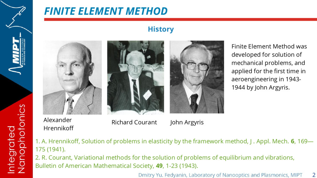
2. 2 FINITE ELEMENT METHOD History 1. A. Hrennikoff, Solution of problems in elasticity by the framework method, J . Appl. Mech. 6, 169— 175 (1941). 2. R. Courant, Variational methods for the solution of problems of equilibrium and vibrations, Bulletin of American Mathematical Society, 49, 1-23 (1943). Alexander Hrennikoff Richard Courant John Argyris Finite Element Method was developed for solution of mechanical problems, and applied for the first time in aeroengineering in 1943- 1944 by John Argyris.
3. 3 FINITE ELEMENT METHOD Basics • FEM is used for solution of boundary value problems for partial differential equations • Supports meshes with different density • Arbitrary forms
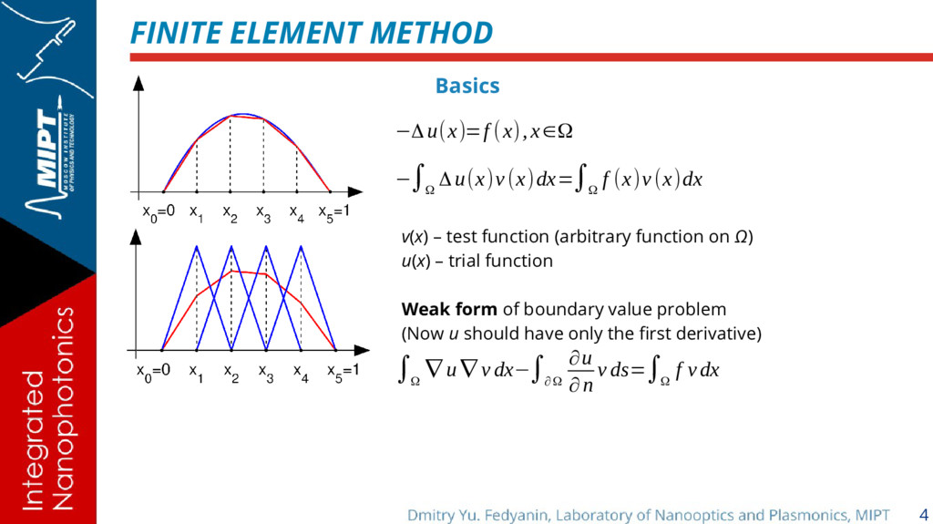
4. 4 FINITE ELEMENT METHOD Basics −Δu(x)=f (x), x∈Ω −∫ Ω Δu(x)v(x)dx=∫ Ω f (x)v(x)dx v(x) – test function (arbitrary function on Ω) u(x) – trial function Weak form of boundary value problem (Now u should have only the first derivative) ∫ Ω ∇ u ∇ v dx−∫ ∂ Ω ∂u ∂n v ds=∫ Ω f vdx
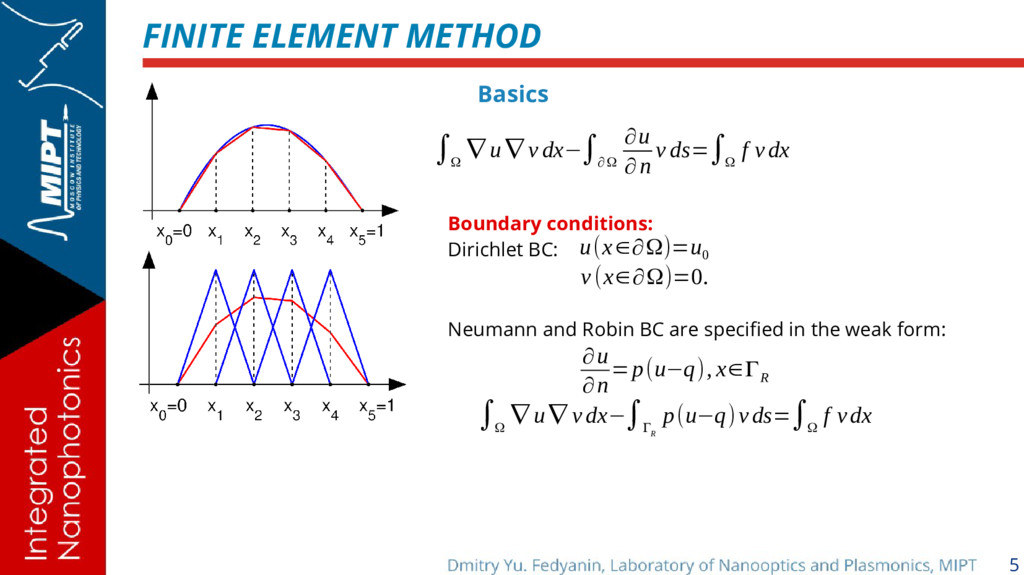
5. 5 FINITE ELEMENT METHOD Basics ∫ Ω ∇ u ∇ v dx−∫ ∂ Ω ∂u ∂n v ds=∫ Ω f vdx Boundary conditions: Dirichlet BC: Neumann and Robin BC are specified in the weak form: u(x∈∂Ω)=u 0 v(x∈∂Ω)=0. ∫ Ω ∇ u ∇ v dx−∫ Γ R p(u−q)vds=∫ Ω f vdx ∂u ∂n =p(u−q), x∈Γ R
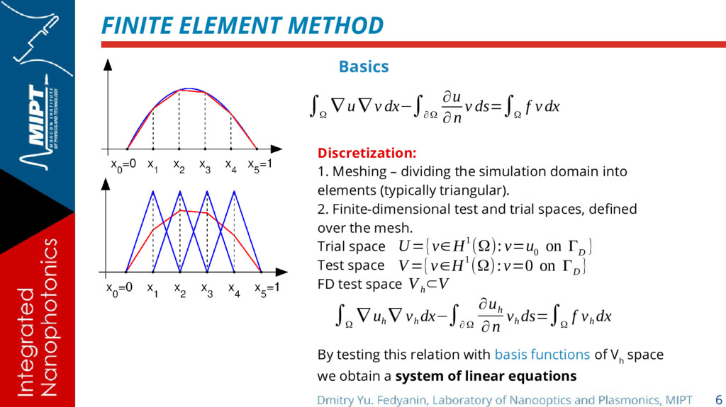
6. 6 FINITE ELEMENT METHOD Basics ∫ Ω ∇ u ∇ v dx−∫ ∂ Ω ∂u ∂n v ds=∫ Ω f vdx Discretization: 1. Meshing – dividing the simulation domain into elements (typically triangular). 2. Finite-dimensional test and trial spaces, defined over the mesh. Trial space Test space FD test space U={v∈H1(Ω):v=u 0 on Γ D } V={v∈H1(Ω):v=0 on Γ D } V h ⊂V ∫ Ω ∇ u h ∇ v h dx−∫ ∂ Ω ∂u h ∂n v h ds=∫ Ω f v h dx By testing this relation with basis functions of V h space we obtain a system of linear equations
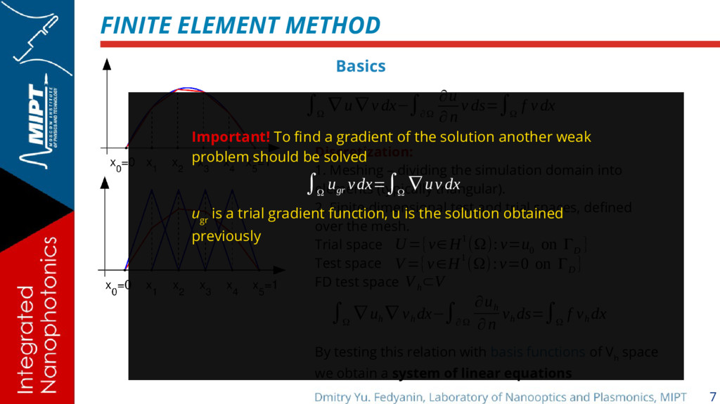
7. 7 FINITE ELEMENT METHOD Basics ∫ Ω ∇ u ∇ v dx−∫ ∂ Ω ∂u ∂n v ds=∫ Ω f vdx Discretization: 1. Meshing – dividing the simulation domain into elements (typically triangular). 2. Finite-dimensional test and trial spaces, defined over the mesh. Trial space Test space FD test space U={v∈H1(Ω):v=u 0 on Γ D } V={v∈H1(Ω):v=0 on Γ D } V h ⊂V ∫ Ω ∇ u h ∇ v h dx−∫ ∂ Ω ∂u h ∂n v h ds=∫ Ω f v h dx By testing this relation with basis functions of V h space we obtain a system of linear equations Important! To find a gradient of the solution another weak problem should be solved u gr is a trial gradient function, u is the solution obtained previously ∫ Ω u gr vdx=∫ Ω ∇ uv dx
8. 8 FINITE ELEMENT METHOD Case study Δu=−1, u(0)=1,u'(1)=−1
9. 9 FINITE ELEMENT METHOD Case study Δu=−1, u(0)=1,u'(1)=−1 u=−x2/2+C 1 x+C 2 u=−x2/2+1
10. 10 FINITE ELEMENT METHOD Case study Δu=−1, u(0)=1,u'(1)=−1 ∫ 0 1 u' v' dx=∫ 0 1 vdx−v(1), v(0)=0 u=−x2/2+C 1 x+C 2 u=−x2/2+1 ∫ 0 1 u' ' vdx=−∫ 0 1 vdx , v(0)=0
11. 11 FINITE ELEMENT METHOD Case study Δu=−1, u(0)=1,u'(1)=−1 ∫ 0 1 u' v' dx=∫ 0 1 vdx−v(1), v(0)=0 u=−x2/2+C 1 x+C 2 u=−x2/2+1 ∫ 0 1 u' ' vdx=−∫ 0 1 vdx , v(0)=0 X = 0, 1/3, 2/3, 1 u 0 , u 1 , u 2 , u 3 v 1 (0)=0 v 1 (1/3)=1 v 1 (2/3)=0
12. 12 FINITE ELEMENT METHOD Case study Δu=−1, u(0)=1,u'(1)=−1 ∫ 0 1 u' v' dx=∫ 0 1 vdx−v(1), v(0)=0 u=−x2/2+C 1 x+C 2 u=−x2/2+1 ∫ 0 1 u' ' vdx=−∫ 0 1 vdx , v(0)=0 X = 0, 1/3, 2/3, 1 u 0 , u 1 , u 2 , u 3 v 1 (0)=0 v 1 (1/3)=1 v 1 (2/3)=0 {v 0 : u 0 =1, Dirichlet BC v 1 : 3(u 1 −u 0 )∗3∗1/3−3(u 2 −u 1 )∗3∗1/3=1/3, v 2 : 3(u 2 −u 1 )∗3∗1/3−3(u 3 −u 2 )∗3∗1/3=1/3, v 3 : 3(u 3 −u 2 )∗3∗1/3=1/6−1 u' v' dx
13. 13 FINITE ELEMENT METHOD Case study Δu=−1, u(0)=1,u'(1)=−1 ∫ 0 1 u' v' dx=∫ 0 1 vdx−v(1), v(0)=0 u=−x2/2+C 1 x+C 2 u=−x2/2+1 ∫ 0 1 u' ' vdx=−∫ 0 1 vdx , v(0)=0 X = 0, 1/3, 2/3, 1 u 0 , u 1 , u 2 , u 3 v 1 (0)=0 v 1 (1/3)=1 v 1 (2/3)=0 {v 0 : u 0 =1, Dirichlet BC v 1 : 3(u 1 −u 0 )∗3∗1/3−3(u 2 −u 1 )∗3∗1/3=1/3, v 2 : 3(u 2 −u 1 )∗3∗1/3−3(u 3 −u 2 )∗3∗1/3=1/3, v 3 : 3(u 3 −u 2 )∗3∗1/3=1/6−1 {u 0 =1, (u 1 −u 0 )−(u 2 −u 1 )=1/9, (u 2 −u 1 )−(u 3 −u 2 )=1/9, u 3 −u 2 =−5/18 u 2 −u 1 =−3/18 u 1 −u 0 =−1/18 {u 0 =1, u 1 =17/18, u 2 =14/18=7/9, u 3 =9/18=1/2 Matches the exact solution !
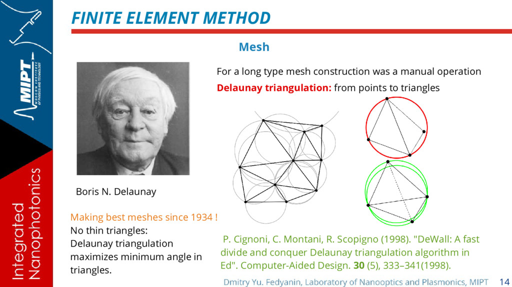
14. 14 FINITE ELEMENT METHOD Mesh Boris N. Delaunay Delaunay triangulation: from points to triangles For a long type mesh construction was a manual operation Making best meshes since 1934 ! No thin triangles: Delaunay triangulation maximizes minimum angle in triangles. P. Cignoni, C. Montani, R. Scopigno (1998). "DeWall: A fast divide and conquer Delaunay triangulation algorithm in Ed". Computer-Aided Design. 30 (5), 333–341(1998).
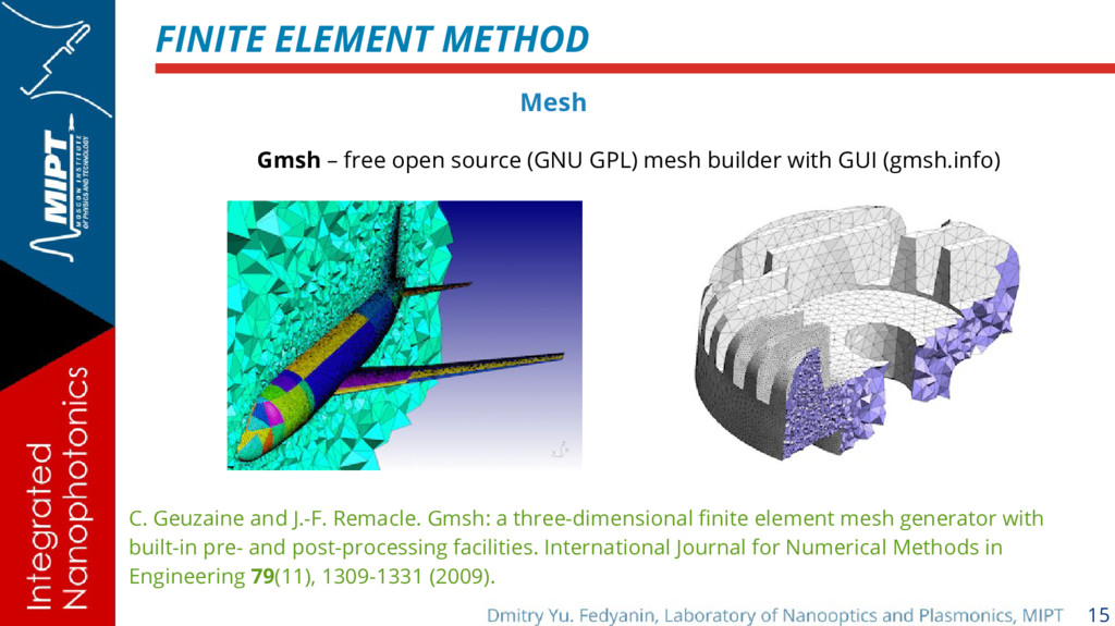
15. 15 FINITE ELEMENT METHOD Mesh Gmsh – free open source (GNU GPL) mesh builder with GUI (gmsh.info) C. Geuzaine and J.-F. Remacle. Gmsh: a three-dimensional finite element mesh generator with built-in pre- and post-processing facilities. International Journal for Numerical Methods in Engineering 79(11), 1309-1331 (2009).
16. 16 FINITE ELEMENT METHOD Packages COMSOL Multiphysics (RF module) FeniCS SimScale FreeFEM++, FEATFLOW CFD, FreeCAD, etc. Nice pictures for your results:
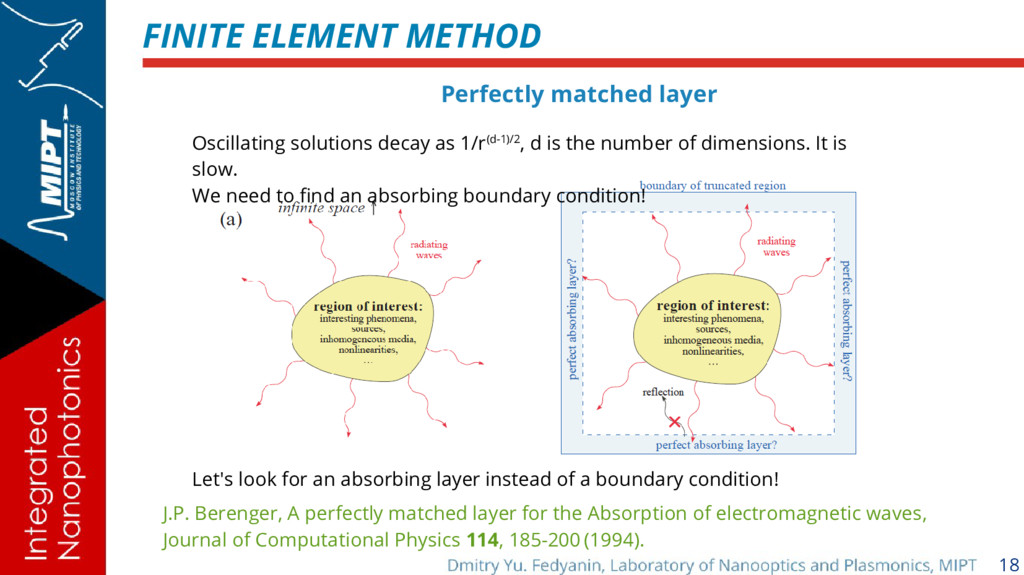
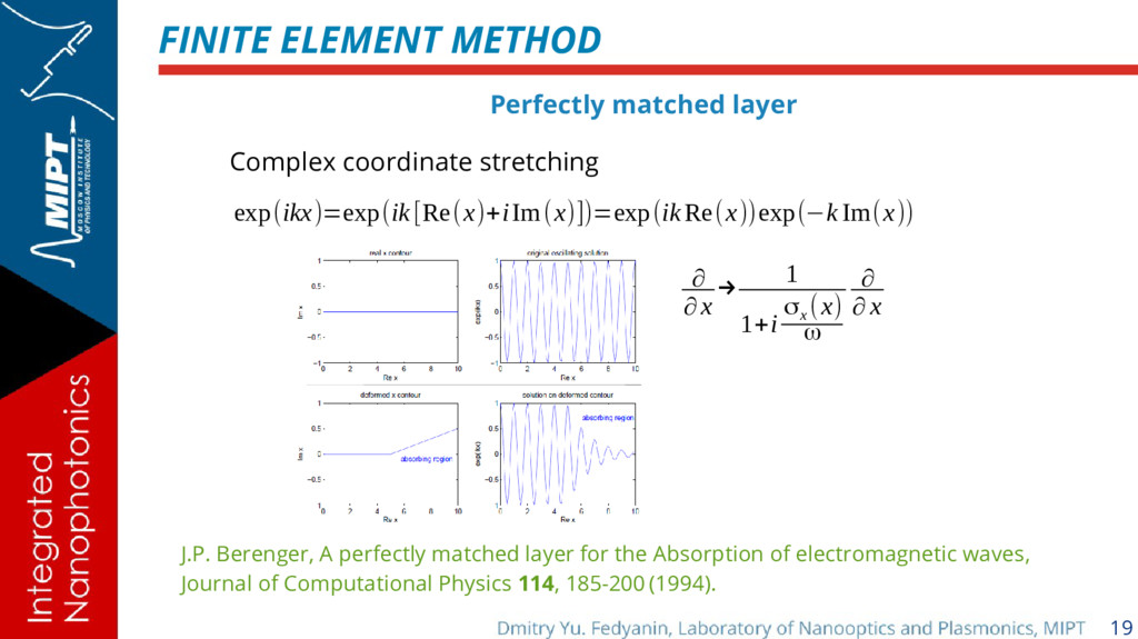
17. 18 FINITE ELEMENT METHOD Perfectly matched layer J.P. Berenger, A perfectly matched layer for the Absorption of electromagnetic waves, Journal of Computational Physics 114, 185-200 (1994). Oscillating solutions decay as 1/r(d-1)/2, d is the number of dimensions. It is slow. We need to find an absorbing boundary condition! Let's look for an absorbing layer instead of a boundary condition!
18. 19 FINITE ELEMENT METHOD Perfectly matched layer J.P. Berenger, A perfectly matched layer for the Absorption of electromagnetic waves, Journal of Computational Physics 114, 185-200 (1994). Complex coordinate stretching exp(ikx)=exp(ik [Re(x)+iIm(x)])=exp(ik Re(x))exp(−k Im(x)) ∂ ∂ x → 1 1+i σx (x) ω ∂ ∂ x
19. 20 FINITE ELEMENT METHOD Perfectly matched layer What are the material properties of PML? σ x is the conductivity (both electric and “magnetic”, because we do not need to restrict ourselves to real materials in simulations) σ y = 0 which means than our material is an anisotropic absorber (uniaxial). PML does not influence evanescent waves exp(-γx). We can increase decay if let σ x be a complex value. ∂ ∂ x → 1 1+i σx (x) ω ∂ ∂ x
20. 21 FINITE ELEMENT METHOD Perfectly matched layer Where PML fails? • Photonic crystals • Metals (negative dielectric permittivity) • Systems with backward waves (phase and group velocities have opposite directions)
21. 22 FINITE ELEMENT METHOD Literature A. Logg, K.-A. Mardal, G. N. Wells et al., Automated Solution of Differential Equations by the Finite Element Method, Springer, (2012) aka The FeniCS book NASA Technical Paper 3485, C. J. Reddy et al., Finite element method for eigenvalue problems in electromagnetics (1994) http://www.eecs.wsu.edu/~schneidj/ufdtd/chap11.pdf