Lecture course "Integrated Nanophotonics" by Dmitry Fedyanin

Lecture 5: Guiding Light (Part 2)

Transcript

1. Integrated Nanophotonics Dmitry Yu. Fedyanin Laboratory of Nanooptics and Plasmonics, MIPT Lecture 5: Guiding Light (Part 2)
2. 2 WHERE DID WE STOP? TM wave TE wave e−4 κ 1 a= κ 1 +κ 2 κ 1 −κ 2 κ 1 +κ 3 κ 1 −κ 3 e−4 κ1 a= κ 1 ε 2 +κ 2 ε 1 κ 1 ε 2 −κ 2 ε 1 κ 1 ε 3 +κ 3 ε 1 κ 1 ε 3 −κ 3 ε 1 κ1 = √β2−(ω c )2 ε1 κ2 = √β2−(ω c )2 ε2 κ 3 = √β2−(ω c )2 ε 3
3. 3 DISPERSION RELATION TE wave ε 2 =ε 3 Symmetric structure tanh(κ 1 a)=− κ 2 ε 1 κ 1 ε 2 tanh(κ 1 a)=− κ 1 ε 2 κ 2 ε 1 tanh(κ 1 a)=− κ 2 κ 1 tanh(κ 1 a)=− κ 1 κ 2 e−4 κ 1 a= κ 1 +κ 2 κ 1 −κ 2 κ 1 +κ 3 κ 1 −κ 3 TM wave e−4 κ1 a= κ 1 ε 2 +κ 2 ε 1 κ 1 ε 2 −κ 2 ε 1 κ 1 ε 3 +κ 3 ε 1 κ 1 ε 3 −κ 3 ε 1
4. 4 DISPERSION RELATION Different approach wikipedia β=k n 1 sinθ, sin θ >sin θ TIR ≥ n 2 n 1 , n 3 n 1
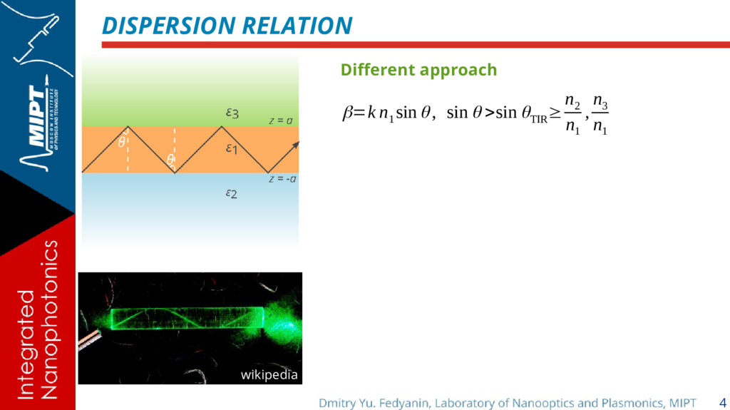
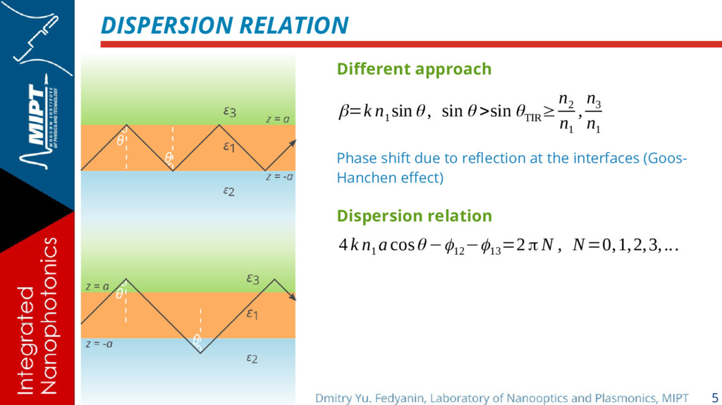
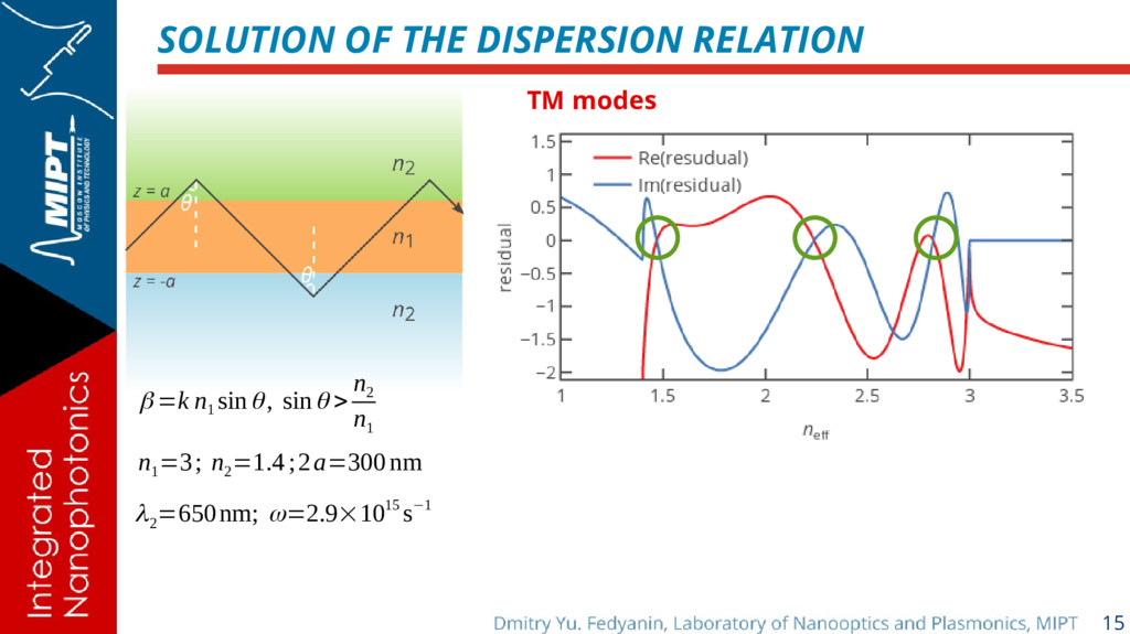
5. 5 DISPERSION RELATION Different approach β=k n 1 sinθ, sin θ >sin θ TIR ≥ n 2 n 1 , n 3 n 1 Phase shift due to reflection at the interfaces (Goos- Hanchen effect) Dispersion relation 4 k n 1 a cosθ −ϕ 12 −ϕ 13 =2 π N , N=0,1,2,3,...
6. 6 RADIATION MODES if β < ω c n 2 (θ<θTIR ), then κ2 2=β2−(ω c )2 n 2 2 < 0
7. 7 RADIATION MODES if β < ω c n 2 (θ<θTIR ), then κ2 2=β2−(ω c )2 n 2 2 < 0 Important: all modes, both guided and radiation, are orthogonal to each other.
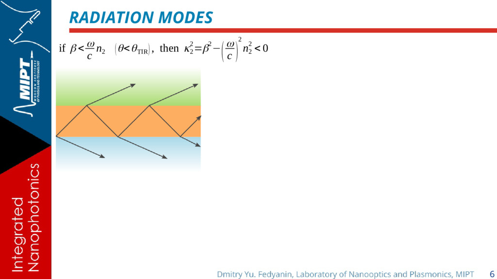
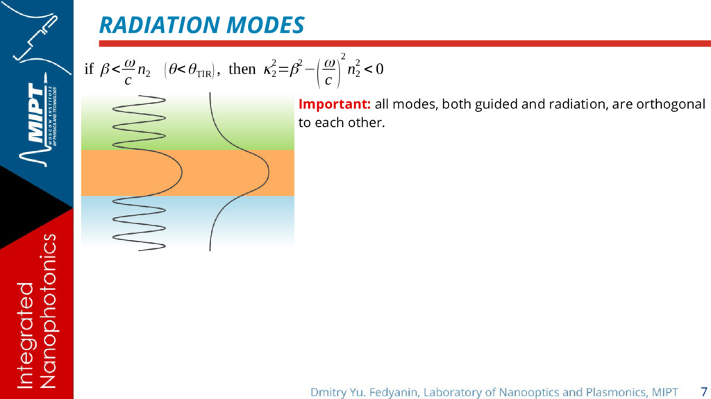
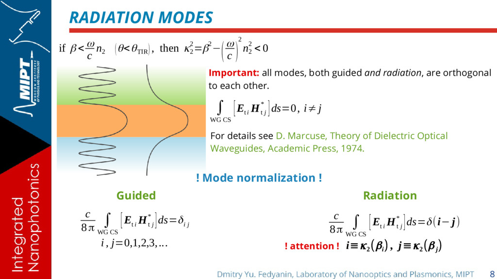
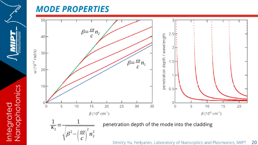
8. 8 RADIATION MODES if β < ω c n 2 (θ<θTIR ), then κ2 2=β2−(ω c )2 n 2 2 < 0 Important: all modes, both guided and radiation, are orthogonal to each other. For details see D. Marcuse, Theory of Dielectric Optical Waveguides, Academic Press, 1974. ∫ WG CS [E t i H t j * ]ds=0, i≠ j ! Mode normalization ! Guided Radiation c 8π ∫ WG CS [E t i H t j * ]ds=δ i j i , j=0,1,2,3,... c 8π ∫ WG CS [E ti H t j * ]ds=δ(i− j) i≡κ2 (βi ) , j≡κ2 (β j ) ! attention !
9. 9 SOLUTION OF THE DISPERSION RELATION TM modes residual=e−4 κ1 a− κ 1 ε 2 +κ 2 ε 1 κ 1 ε 2 −κ 2 ε 1 κ 1 ε 3 +κ 3 ε 1 κ 1 ε 3 −κ 3 ε 1 β =k n 1 sinθ, sinθ > n 2 n 1 n 1 =3; n 2 =1.4 ;2a=300 nm λ 1 =1550 nm; ω=1.216×1015s−1
10. 10 SOLUTION OF THE DISPERSION RELATION β =k n 1 sin θ, sinθ > n 2 n 1 n 1 =3; n 2 =1.4 ;2a=300 nm TM modes residual=e−4 κ1 a− κ 1 ε 2 +κ 2 ε 1 κ 1 ε 2 −κ 2 ε 1 κ 1 ε 3 +κ 3 ε 1 κ 1 ε 3 −κ 3 ε 1 λ 1 =1550 nm; ω=1.216×1015 s−1
11. 11 SOLUTION OF THE DISPERSION RELATION TM modes residual=e−4 κ1 a− κ 1 ε 2 +κ 2 ε 1 κ 1 ε 2 −κ 2 ε 1 κ 1 ε 3 +κ 3 ε 1 κ 1 ε 3 −κ 3 ε 1 β =k n 1 sinθ, sinθ > n 2 n 1 n 1 =3; n 2 =1.4 ;2a=300 nm λ 1 =1550 nm; ω=1.216×1015s−1
12. 12 SOLUTION OF THE DISPERSION RELATION TM modes residual=e−4 κ1 a− κ 1 ε 2 +κ 2 ε 1 κ 1 ε 2 −κ 2 ε 1 κ 1 ε 3 +κ 3 ε 1 κ 1 ε 3 −κ 3 ε 1 β =k n 1 sinθ, sinθ > n 2 n 1 n 1 =3; n 2 =1.4 ;2a=300 nm λ 1 =1550 nm; ω=1.216×1015s−1
13. 13 SOLUTION OF THE DISPERSION RELATION β =k n 1 sinθ, sinθ > n 2 n 1 n 1 =3; n 2 =1.4 ;2a=300 nm λ 1 =1550 nm; ω=1.216×1015s−1
14. 14 SOLUTION OF THE DISPERSION RELATION λ 2 =650nm; ω=2.9×1015 s−1 TM modes β =k n 1 sinθ, sinθ > n 2 n 1 n 1 =3; n 2 =1.4 ;2a=300 nm
15. 15 SOLUTION OF THE DISPERSION RELATION TM modes λ 2 =650nm; ω=2.9×1015 s−1 β =k n 1 sinθ, sinθ > n 2 n 1 n 1 =3; n 2 =1.4 ;2a=300 nm
16. 16 SOLUTION OF THE DISPERSION RELATION β =k n 1 sin θ, sinθ > n 2 n 1 n 1 =3; n 2 =1.4 ; 2a=300 nm TM modes β=ω c n 2 β=ω c n 1
17. 17 SOLUTION OF THE DISPERSION RELATION TE modes β=ω c n 2 β=ω c n 1 β =k n 1 sinθ, sinθ > n 2 n 1 n 1 =3; n 2 =1.4 ; 2a=300 nm
18. 18 SOLUTION OF THE DISPERSION RELATION β=ω c n 2 β=ω c n 1 TE and TM modes β =k n 1 sinθ, sinθ > n 2 n 1 n 1 =3; n 2 =1.4 ; 2a=300 nm
19. 19 MODE PROPERTIES TM modes β=ω c n 2 β=ω c n 1 cutoff frequencies β =k n 1 sinθ, sinθ > n 2 n 1 n 1 =3; n 2 =1.4 ; 2a=300 nm
20. 20 MODE PROPERTIES β=ω c n 2 β=ω c n 1 1 κ 2 = 1 √β2−(ω c )2 n 2 2 penetration depth of the mode into the cladding
21. 21 MODE PROPERTIES M S = 1 2 κ2 +2a+ 1 2κ2 =2a+ 1 √β 2−(ω c )2 n 2 2 We can introduce an effective mode size
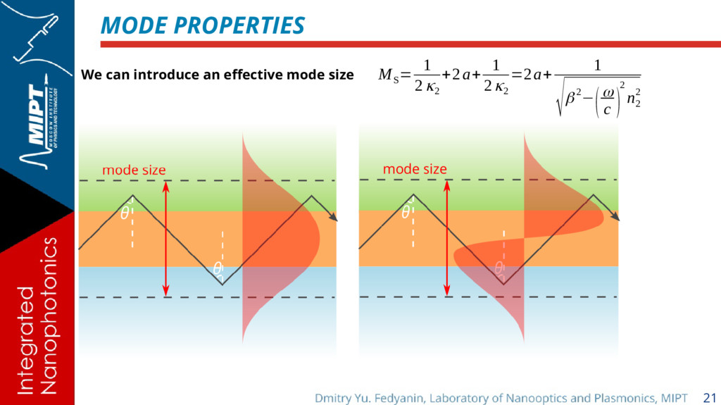
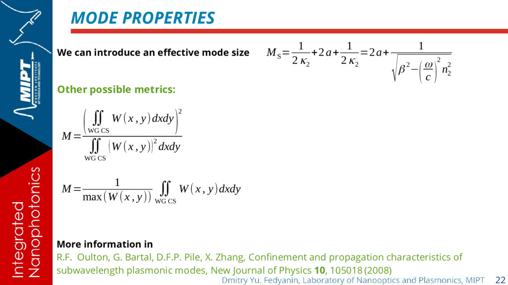
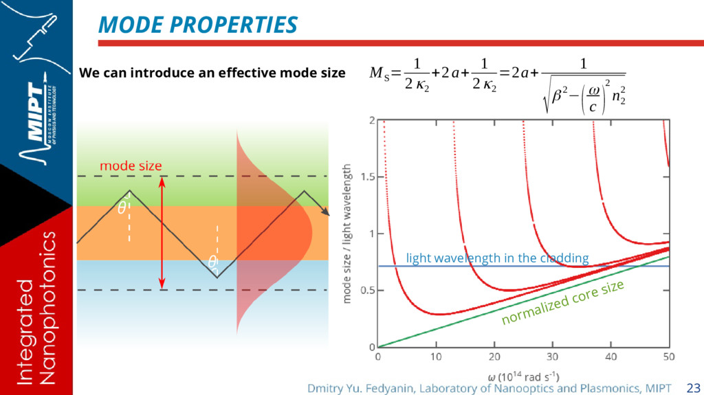
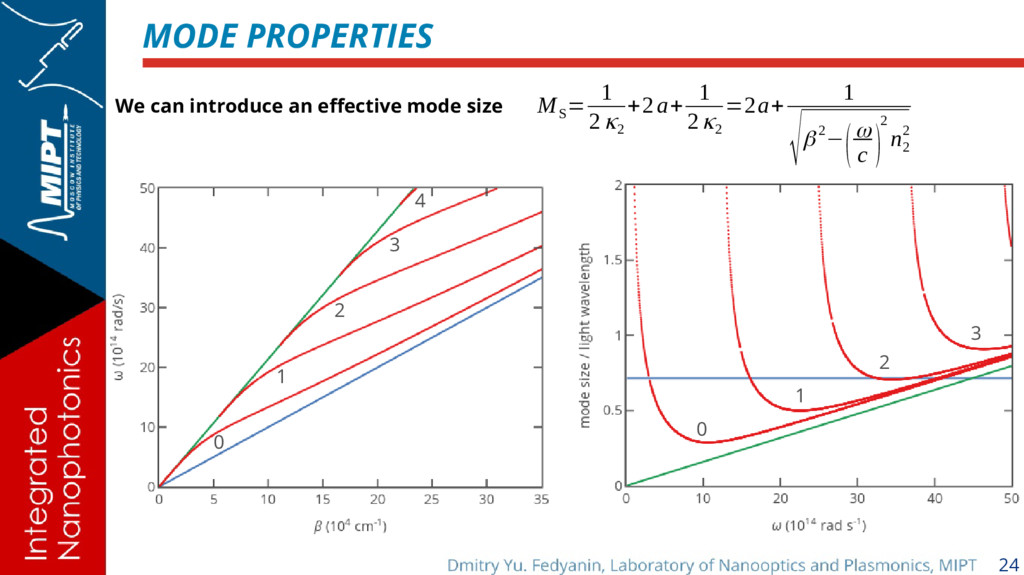
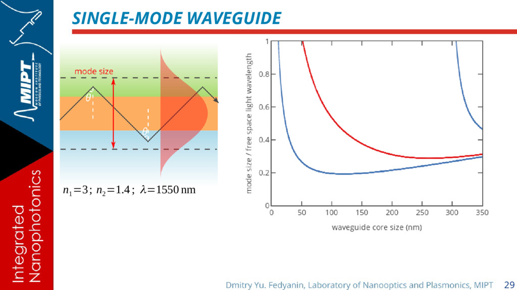
22. 22 MODE PROPERTIES M S = 1 2 κ2 +2a+ 1 2κ2 =2a+ 1 √β 2−(ω c )2 n 2 2 We can introduce an effective mode size Other possible metrics: M= ( ∬ WG CS W (x , y)dxdy)2 ∬ WG CS (W (x , y))2 dxdy M= 1 max(W (x , y)) ∬ WG CS W (x , y)dxdy More information in R.F. Oulton, G. Bartal, D.F.P. Pile, X. Zhang, Confinement and propagation characteristics of subwavelength plasmonic modes, New Journal of Physics 10, 105018 (2008)
23. 23 MODE PROPERTIES light wavelength in the cladding normalized core size M S = 1 2 κ2 +2a+ 1 2κ2 =2a+ 1 √β 2−(ω c )2 n 2 2 We can introduce an effective mode size
24. 24 MODE PROPERTIES 0 1 2 3 4 0 1 2 3 M S = 1 2 κ2 +2a+ 1 2κ2 =2a+ 1 √β 2−(ω c )2 n 2 2 We can introduce an effective mode size
25. 25 MODE PROPERTIES Which mode provides better confinement, TE or TM?
26. 26 MODE PROPERTIES Which mode provides better confinement, TE or TM?
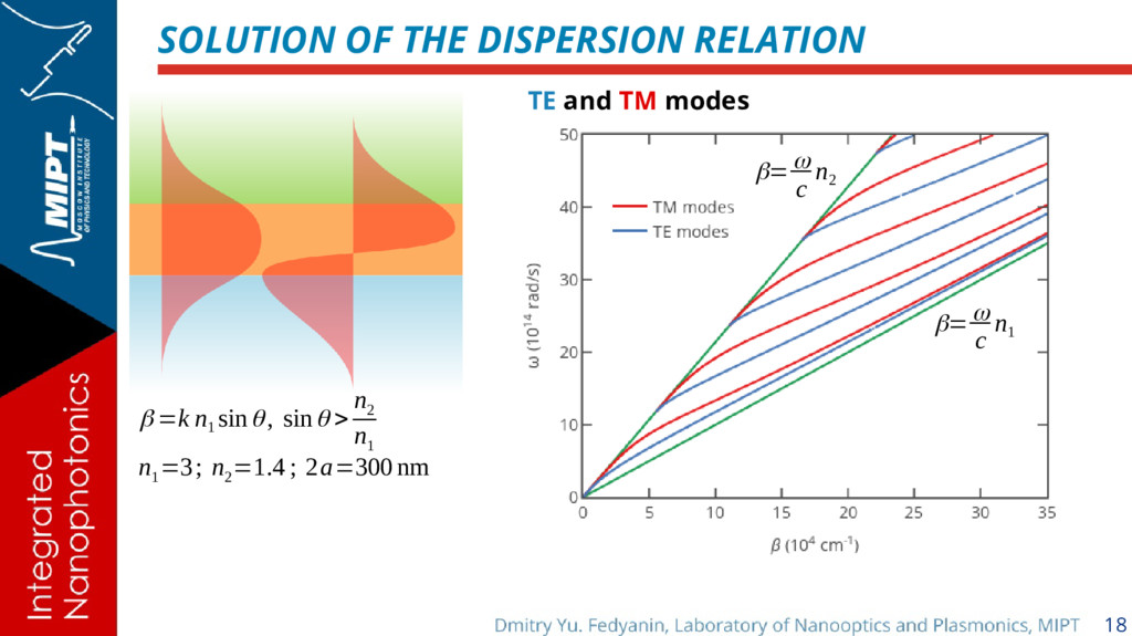
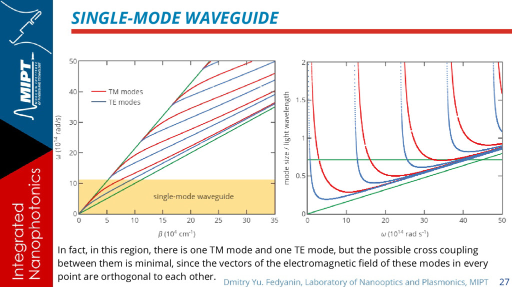
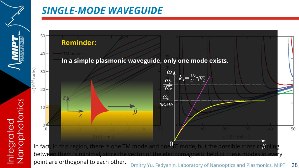
27. 27 SINGLE-MODE WAVEGUIDE In fact, in this region, there is one TM mode and one TE mode, but the possible cross coupling between them is minimal, since the vectors of the electromagnetic field of these modes in every point are orthogonal to each other.
28. 28 SINGLE-MODE WAVEGUIDE In fact, in this region, there is one TM mode and one TE mode, but the possible cross coupling between them is minimal, since the vector of the electromagnetic field of these modes in every point are orthogonal to each other. Reminder: In a simple plasmonic waveguide, only one mode exists.
29. 29 SINGLE-MODE WAVEGUIDE n 1 =3; n 2 =1.4 ; λ=1550 nm
30. 30 3D WAVEGUIDE
31. 31 3D WAVEGUIDE Effective index method
32. 32 3D WAVEGUIDE EIM-1 EIM-2 T. Holmgaard, S.I. Bozhevolnyi Phys.Rev. B 75, 245405 (2007).
33. 33 3D WAVEGUIDE EIM-1 EIM-2 T. Holmgaard, S.I. Bozhevolnyi Phys.Rev. B 75, 245405 (2007).
34. 37 NEXT CLASS Resonators, filters and modulators. Homework: Т. Тамир, Интегральная оптика. — М.: Мир, 1978. T. Tamir, Integrated Optics, Springer, 1975. Chapter 2: Sections 2.1 – 2.5