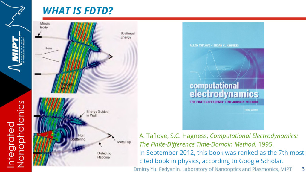
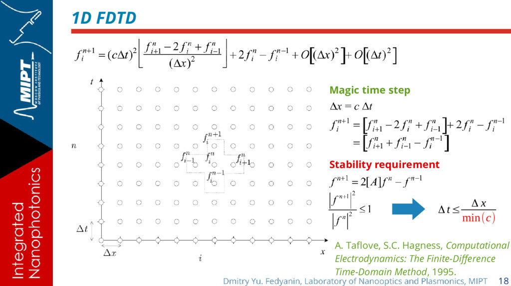
The Finite-Difference Time-Domain Method, 1995. In September 2012, this book was ranked as the 7th most- cited book in physics, according to Google Scholar.
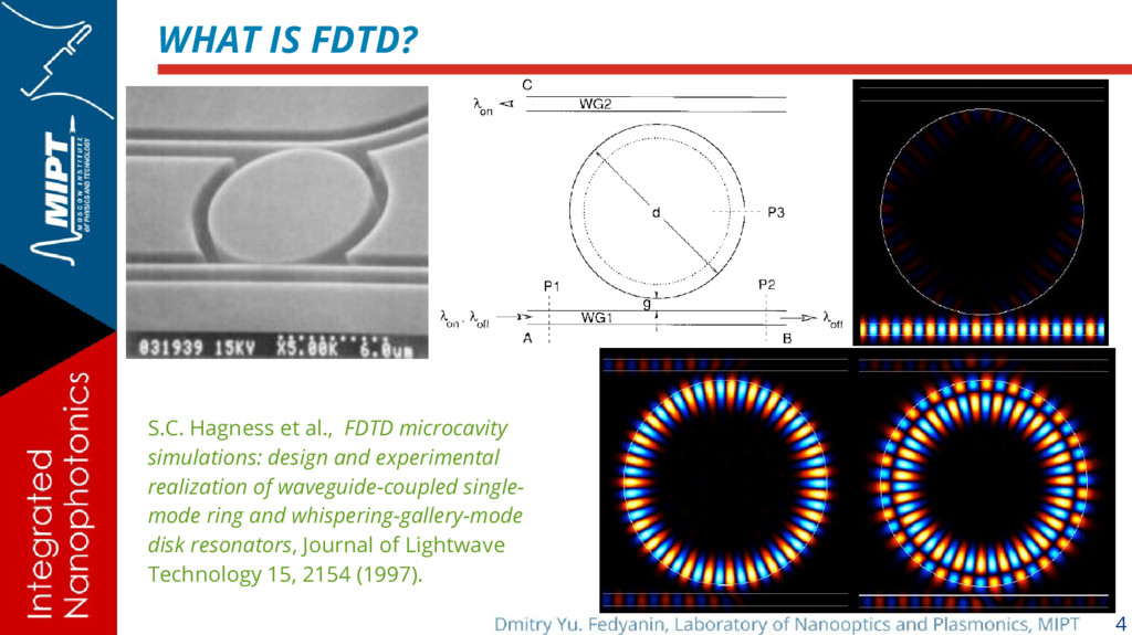
simulations: design and experimental realization of waveguide-coupled single- mode ring and whispering-gallery-mode disk resonators, Journal of Lightwave Technology 15, 2154 (1997).
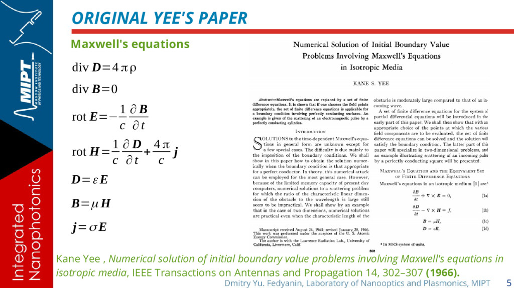
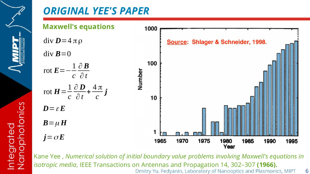
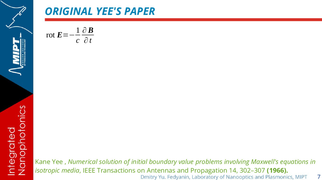
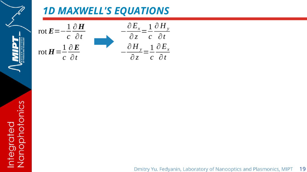
E=− 1 c ∂ B ∂t Maxwell's equations rot H= 1 c ∂ D ∂t + 4 π c j D=ε E B=μ H j=σ E Kane Yee , Numerical solution of initial boundary value problems involving Maxwell's equations in isotropic media, IEEE Transactions on Antennas and Propagation 14, 302–307 (1966).
E=− 1 c ∂ B ∂t Maxwell's equations rot H= 1 c ∂ D ∂t + 4 π c j D=ε E B=μ H j=σ E Kane Yee , Numerical solution of initial boundary value problems involving Maxwell's equations in isotropic media, IEEE Transactions on Antennas and Propagation 14, 302–307 (1966).
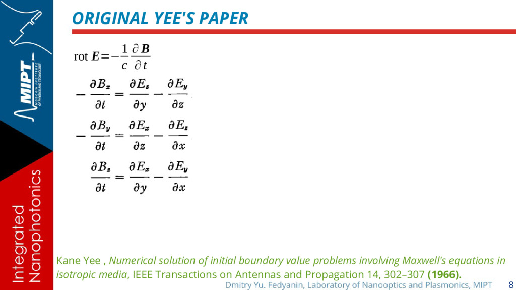
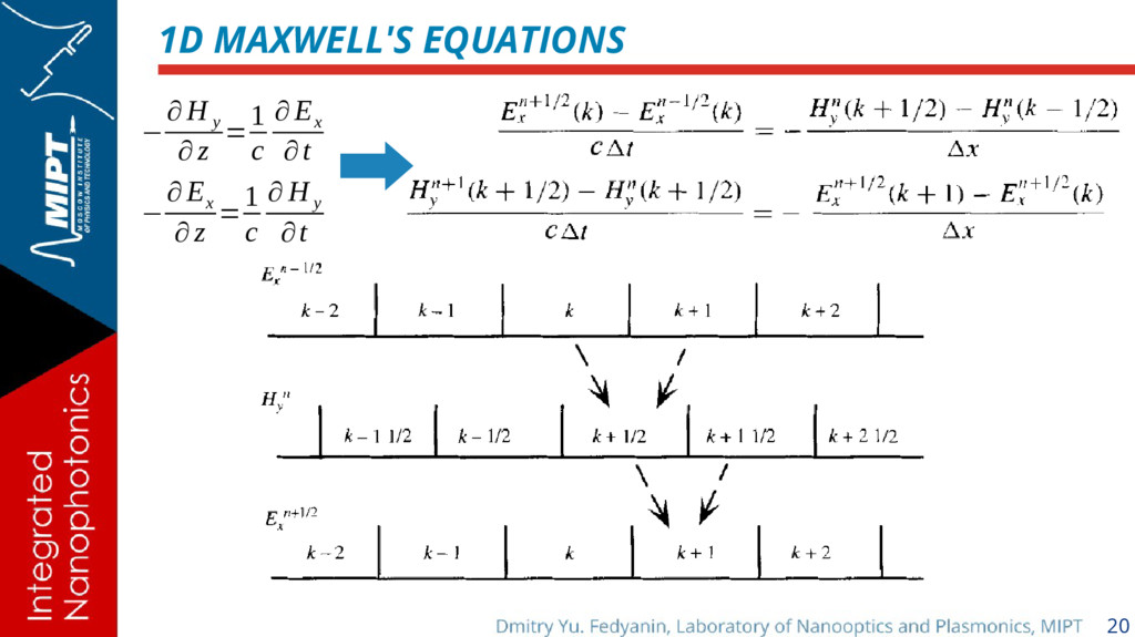
∂t Kane Yee , Numerical solution of initial boundary value problems involving Maxwell's equations in isotropic media, IEEE Transactions on Antennas and Propagation 14, 302–307 (1966).
∂t Kane Yee , Numerical solution of initial boundary value problems involving Maxwell's equations in isotropic media, IEEE Transactions on Antennas and Propagation 14, 302–307 (1966).
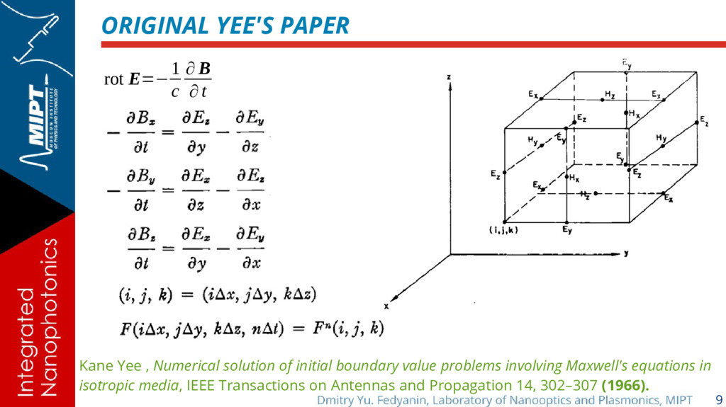
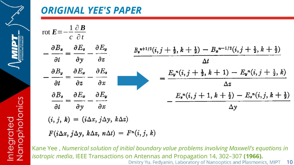
∂t Kane Yee , Numerical solution of initial boundary value problems involving Maxwell's equations in isotropic media, IEEE Transactions on Antennas and Propagation 14, 302–307 (1966).
∂t Kane Yee , Numerical solution of initial boundary value problems involving Maxwell's equations in isotropic media, IEEE Transactions on Antennas and Propagation 14, 302–307 (1966).
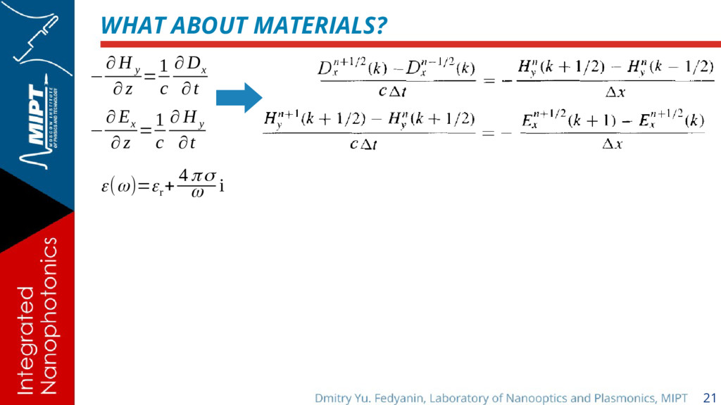
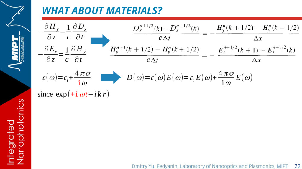
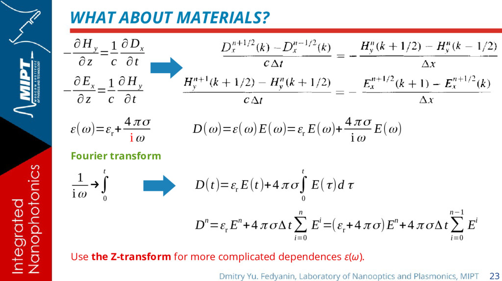
= 1 c ∂ H y ∂t − ∂ H y ∂ z = 1 c ∂ D x ∂t ε(ω)=ε r + 4 πσ i ω D(ω)=ε(ω)E(ω)=ε r E(ω)+ 4 πσ i ω E(ω) Fourier transform 1 iω →∫ 0 t D(t)=ε r E(t)+4 π σ∫ 0 t E(τ)d τ Dn=ε r En+4 πσ Δ t∑ i=0 n Ei=(ε r +4 πσ)En+4 πσ Δ t ∑ i=0 n−1 Ei Use the Z-transform for more complicated dependences ε(ω).
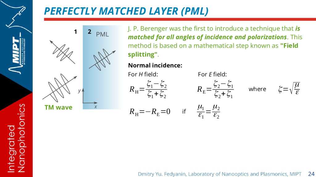
first to introduce a technique that is matched for all angles of incidence and polarizations. This method is based on a mathematical step known as "Field splitting". R H = ζ 1 −ζ 2 ζ 1 +ζ 2 Normal incidence: ζ=√μ ε 1 2 TM wave For H field: R E = ζ 2 −ζ 1 ζ 2 +ζ 1 For E field: where R H =−R E =0 if μ 1 ε 1 = μ 2 ε 2
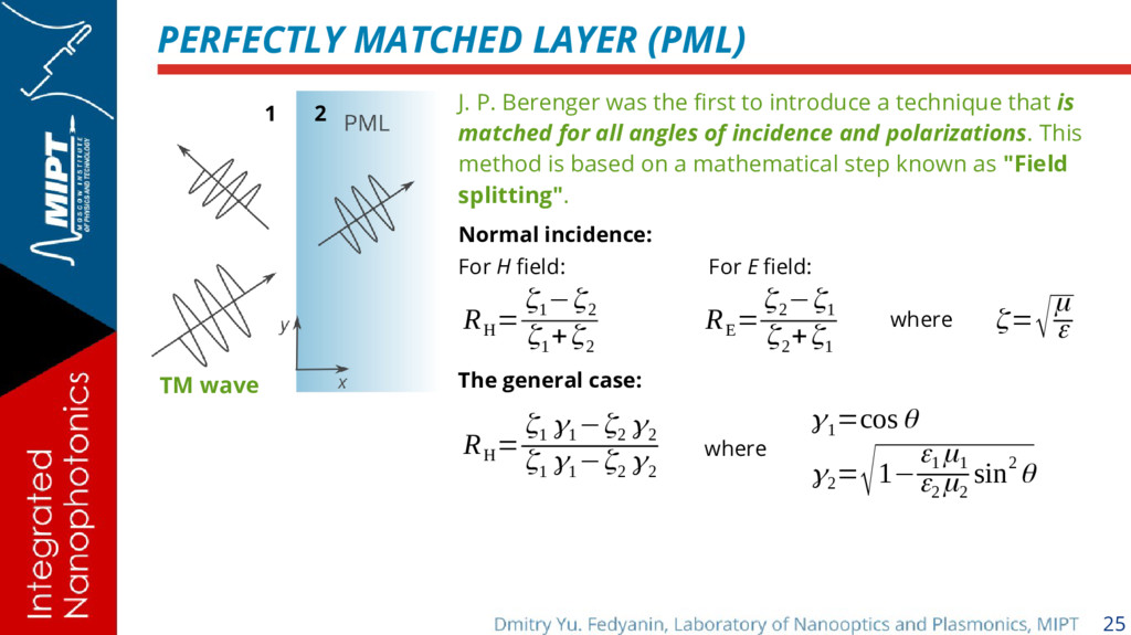
first to introduce a technique that is matched for all angles of incidence and polarizations. This method is based on a mathematical step known as "Field splitting". R H = ζ 1 −ζ 2 ζ 1 +ζ 2 Normal incidence: ζ=√μ ε R H = ζ 1 γ 1 −ζ 2 γ 2 ζ 1 γ 1 −ζ 2 γ 2 1 2 TM wave For H field: R E = ζ 2 −ζ 1 ζ 2 +ζ 1 For E field: The general case: where where γ 1 =cosθ γ 2 = √1− ε 1 μ 1 ε 2 μ 2 sin2θ
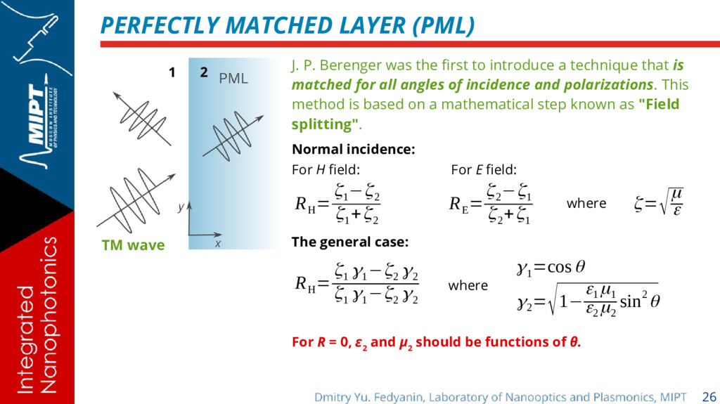
first to introduce a technique that is matched for all angles of incidence and polarizations. This method is based on a mathematical step known as "Field splitting". R H = ζ 1 −ζ 2 ζ 1 +ζ 2 Normal incidence: ζ=√μ ε R H = ζ 1 γ 1 −ζ 2 γ 2 ζ 1 γ 1 −ζ 2 γ 2 1 2 TM wave For H field: R E = ζ 2 −ζ 1 ζ 2 +ζ 1 For E field: The general case: where where γ 1 =cosθ γ 2 = √1− ε 1 μ 1 ε 2 μ 2 sin2θ For R = 0, ε 2 and μ 2 should be functions of θ.
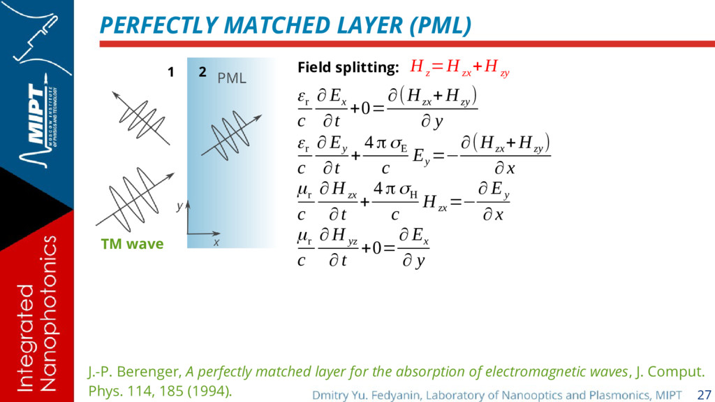
zy Field splitting: 1 2 TM wave J.-P. Berenger, A perfectly matched layer for the absorption of electromagnetic waves, J. Comput. Phys. 114, 185 (1994). ε r c ∂ E x ∂t +0= ∂(H zx +H zy ) ∂ y ε r c ∂ E y ∂t + 4 πσ E c E y =− ∂(H zx +H zy ) ∂ x μ r c ∂ H zx ∂t + 4 πσ H c H zx =− ∂ E y ∂ x μr c ∂ H yz ∂ t +0= ∂ E x ∂ y
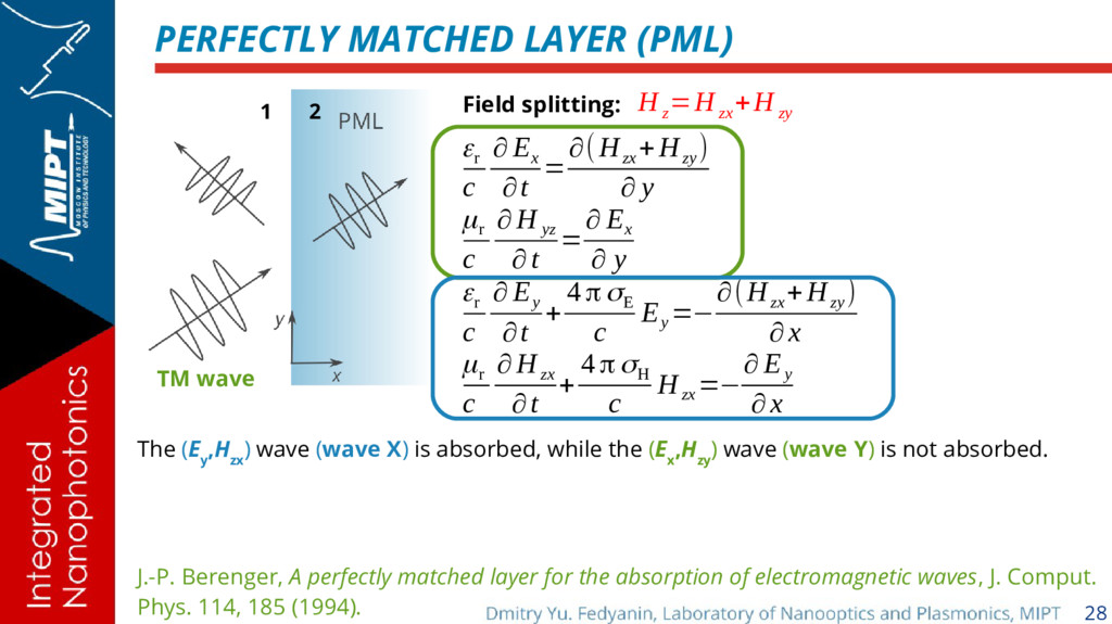
zy ε r c ∂ E x ∂t = ∂(H zx +H zy ) ∂ y μ r c ∂ H yz ∂ t = ∂ E x ∂ y ε r c ∂ E y ∂t + 4 πσ E c E y =− ∂(H zx +H zy ) ∂ x μr c ∂ H zx ∂t + 4 πσH c H zx =− ∂ E y ∂ x Field splitting: 1 2 TM wave J.-P. Berenger, A perfectly matched layer for the absorption of electromagnetic waves, J. Comput. Phys. 114, 185 (1994). The (E y ,H zx ) wave (wave X) is absorbed, while the (E x ,H zy ) wave (wave Y) is not absorbed.
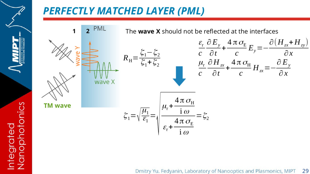
wave X should not be reflected at the interfaces ε r c ∂ E y ∂t + 4 πσ E c E y =− ∂(H zx +H zy ) ∂ x μ r c ∂ H zx ∂t + 4 πσ H c H zx =− ∂ E y ∂ x R H = ζ 1 −ζ 2 ζ 1 +ζ 2 ζ 1 = √μ 1 ε 1 = √μ r + 4πσ H i ω ε r + 4πσ E i ω =ζ 2
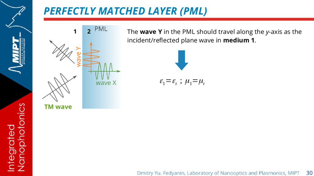
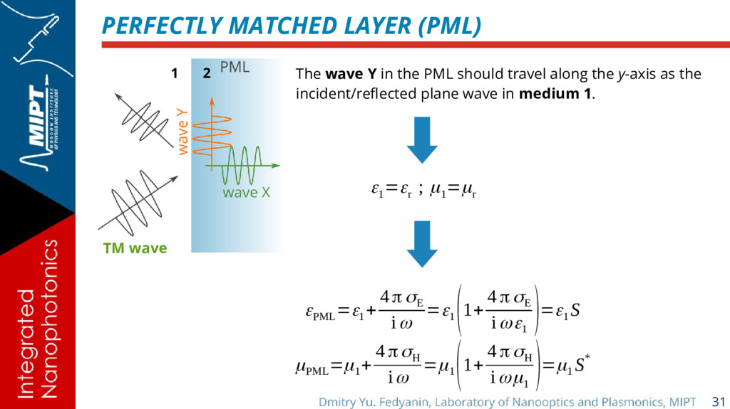
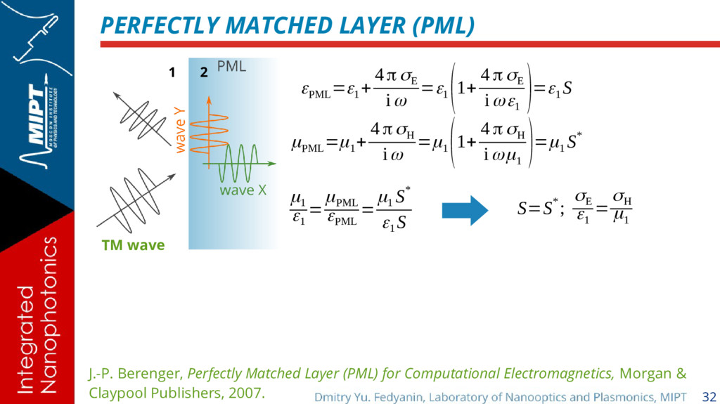
wave Y in the PML should travel along the y-axis as the incident/reflected plane wave in medium 1. ε 1 =ε r ; μ 1 =μ r ε PML =ε 1 + 4πσ E iω =ε 1 (1+ 4 πσ E iωε 1 )=ε 1 S μ PML =μ 1 + 4πσH iω =μ 1 (1+ 4 πσH iωμ 1 )=μ 1 S*
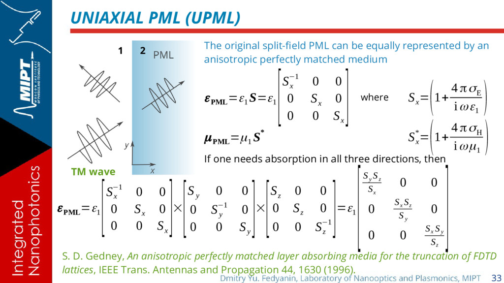
matched layer absorbing media for the truncation of FDTD lattices, IEEE Trans. Antennas and Propagation 44, 1630 (1996). 1 2 TM wave The original split-field PML can be equally represented by an anisotropic perfectly matched medium εPML =ε1 S=ε1 [S x −1 0 0 0 S x 0 0 0 S x ] μPML =μ1 S* If one needs absorption in all three directions, then ε PML =ε 1 [S x −1 0 0 0 S x 0 0 0 S x ]× [S y 0 0 0 S y −1 0 0 0 S y ]× [S z 0 0 0 S z 0 0 0 S z −1 ]=ε 1 [S y S z S x 0 0 0 S x S z S y 0 0 0 S x S y S z ] S x = (1+ 4 πσ E iωε1 ) where S x *= (1+ 4 πσ H iωμ1 )