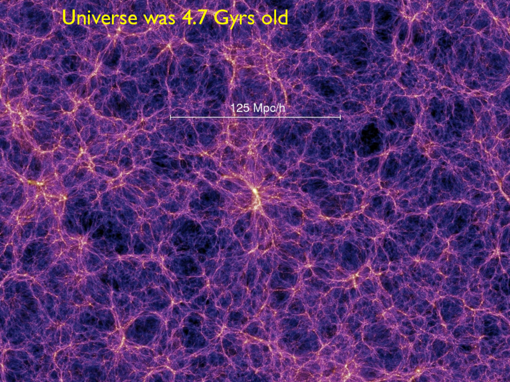
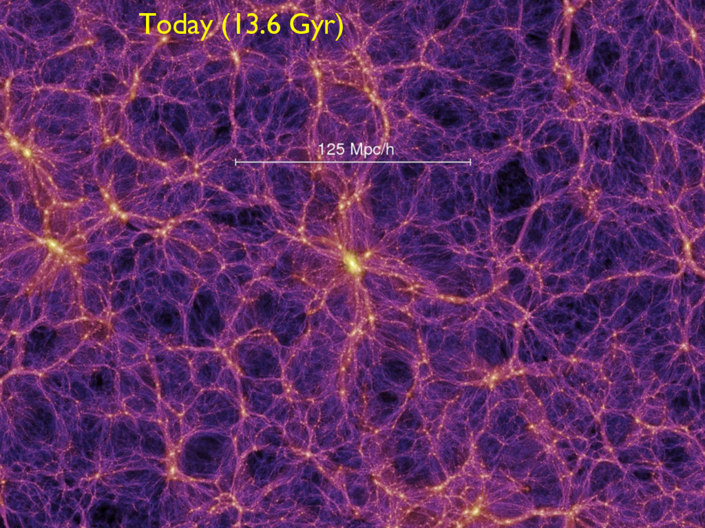
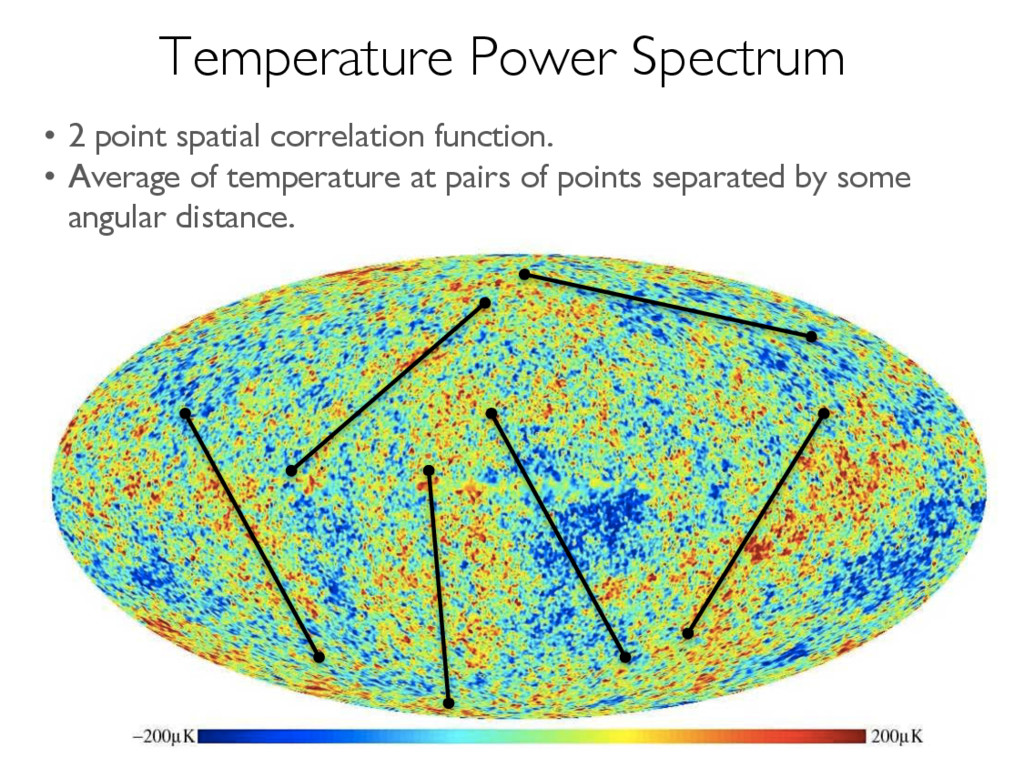
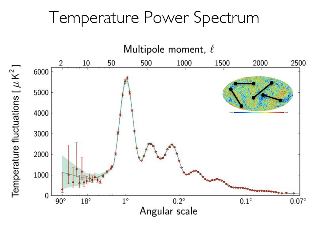
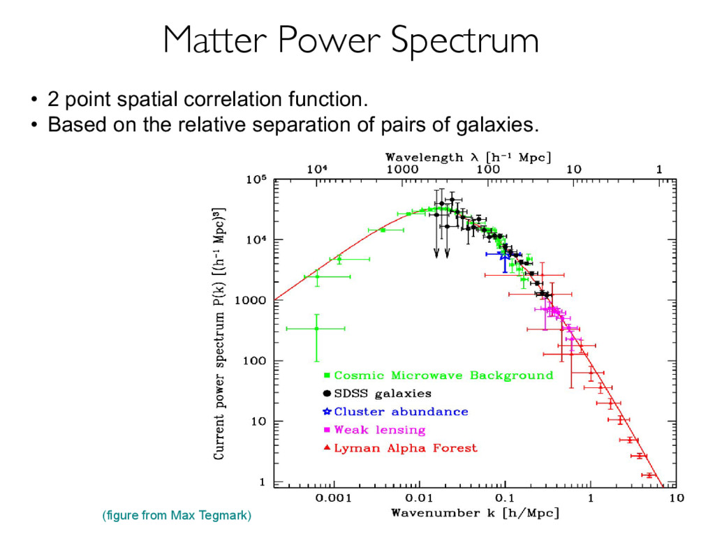
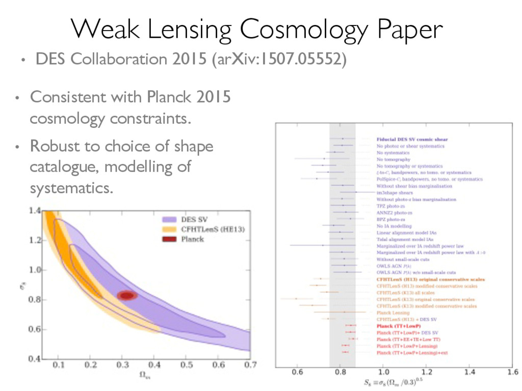
Gaussian random field, we only need to know the power spectrum and the cosmological parameters to describe the ICs DIFFERENT PROBES OF THE MASS POWER SPECTRUM • 2 point spatial correlation function. • Based on the relative separation of pairs of galaxies. Matter Power Spectrum
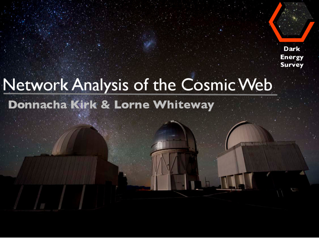
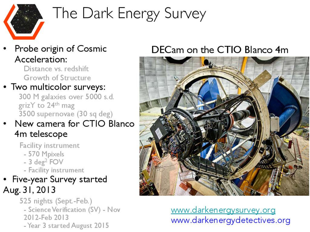
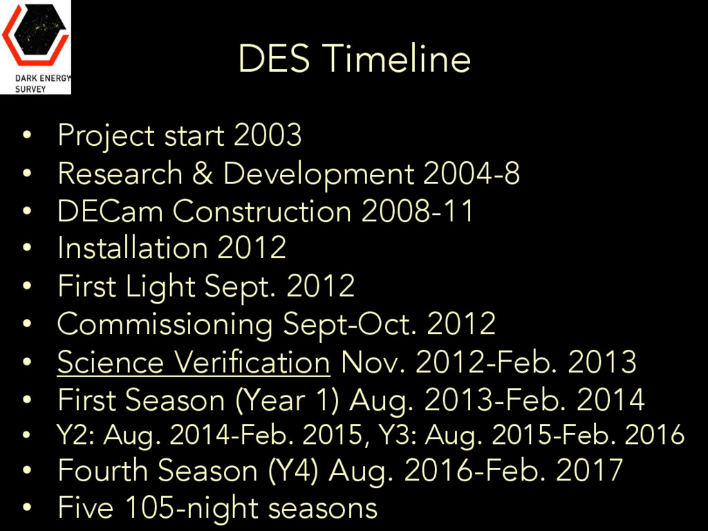
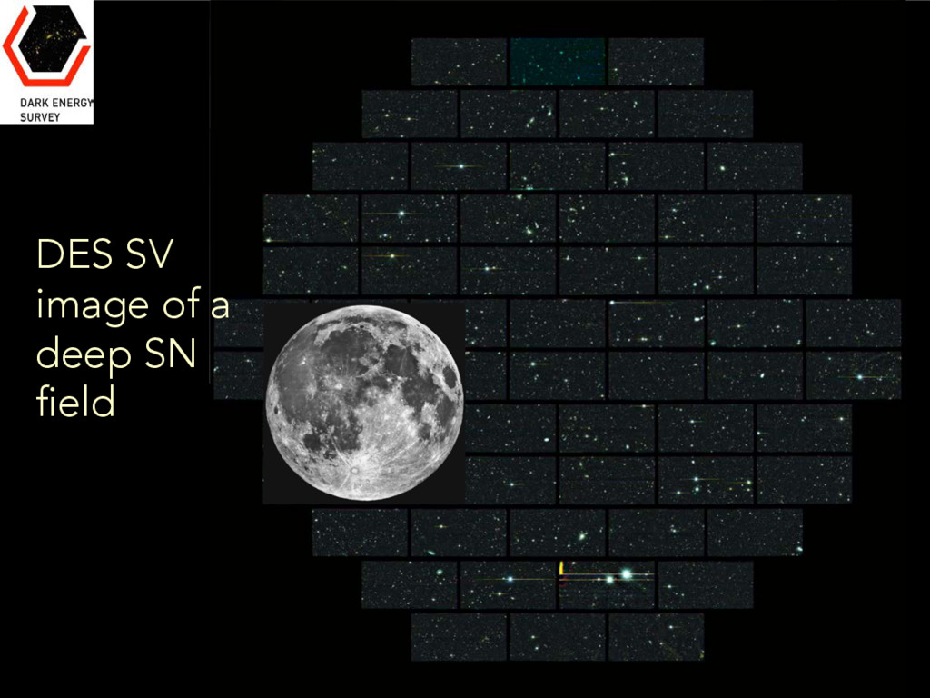
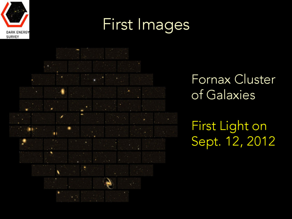
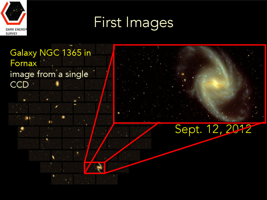
Survey (SPT) DARK ENERGY SURVEY • Probe origin of Cosmic Acceleration: Distance vs. redshift Growth of Structure • Two multicolor surveys: 300 M galaxies over 5000 s.d. grizY to 24th mag 3500 supernovae (30 sq deg) • New camera for CTIO Blanco 4m telescope Facility instrument - 570 Mpixels - 3 deg2 FOV - Facility instrument • Five-year Survey started Aug. 31, 2013 525 nights (Sept.-Feb.) - Science Verification (SV) - Nov 2012-Feb 2013 -Year 3 started August 2015 DECam on the CTIO Blanco 4m www.darkenergysurvey.org www.darkenergydetectives.org
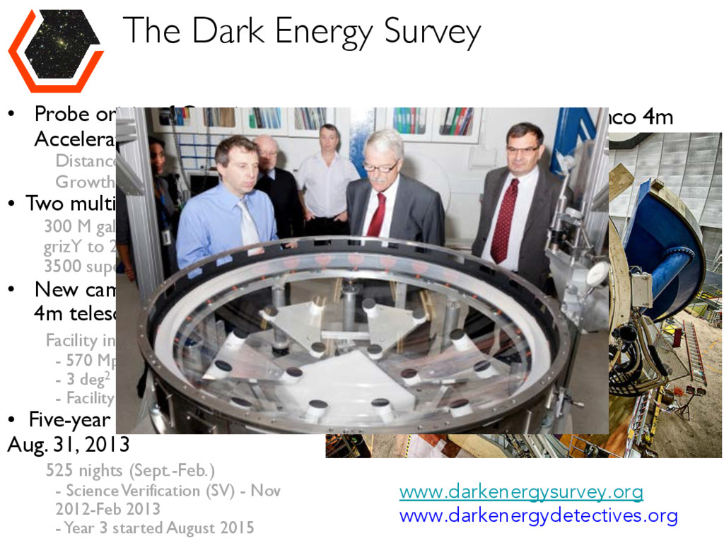
Survey (SPT) DARK ENERGY SURVEY • Probe origin of Cosmic Acceleration: Distance vs. redshift Growth of Structure • Two multicolor surveys: 300 M galaxies over 5000 s.d. grizY to 24th mag 3500 supernovae (30 sq deg) • New camera for CTIO Blanco 4m telescope Facility instrument - 570 Mpixels - 3 deg2 FOV - Facility instrument • Five-year Survey started Aug. 31, 2013 525 nights (Sept.-Feb.) - Science Verification (SV) - Nov 2012-Feb 2013 -Year 3 started August 2015 DECam on the CTIO Blanco 4m www.darkenergysurvey.org www.darkenergydetectives.org
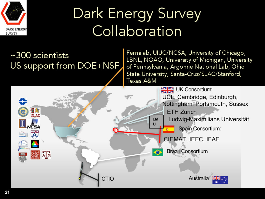
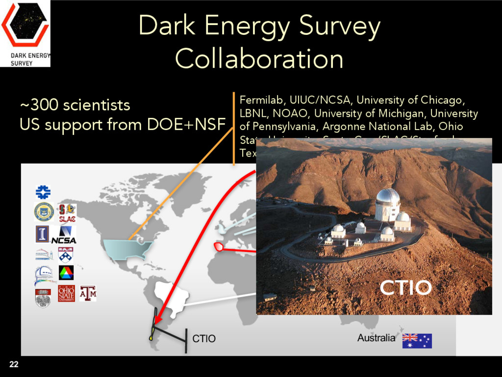
LBNL, NOAO, University of Michigan, University of Pennsylvania, Argonne National Lab, Ohio State University, Santa-Cruz/SLAC/Stanford, Texas A&M Brazil Consortium UK Consortium: UCL, Cambridge, Edinburgh, Nottingham, Portsmouth, Sussex Spain Consortium: CIEMAT, IEEC, IFAE CTIO Ludwig-Maximilians Universität LM U ETH Zurich ~300 scientists US support from DOE+NSF Australia
LBNL, NOAO, University of Michigan, University of Pennsylvania, Argonne National Lab, Ohio State University, Santa-Cruz/SLAC/Stanford, Texas A&M Brazil Consortium UK Consortium: UCL, Cambridge, Edinburgh, Nottingham, Portsmouth, Sussex Spain Consortium: CIEMAT, IEEC, IFAE CTIO Ludwig-Maximilians Universität LM U ETH Zurich ~300 scientists US support from DOE+NSF Australia CTIO
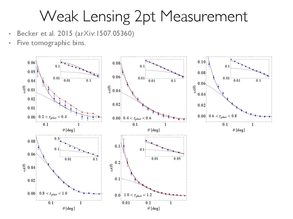
Galaxy clustering, photo-z and systematics in DES-SV 13 Ê Ê Ê Ê Ê Ê Ê Ê Ê Ê Ê Ê Ê ‡ ‡ ‡ ‡ ‡ ‡ ‡ ‡ ‡ ‡ ‡ ‡ ‡ 0.1 1 0.00 0.01 0.02 0.03 0.04 0.05 0.06 q @degD wHqL Ê Ê Ê Ê Ê Ê Ê Ê Ê Ê Ê Ê Ê Ê 0.01 0.1 0.01 0.1 0.2 < zphot < 0.4 Ê Ê Ê Ê Ê Ê Ê Ê Ê Ê Ê Ê Ê Ê ‡ ‡ ‡ ‡ ‡ ‡ ‡ ‡ ‡ ‡ ‡ ‡ ‡ ‡ 0.1 1 0.00 0.02 0.04 0.06 0.08 q @degD wHqL Ê Ê Ê Ê Ê Ê Ê Ê Ê Ê Ê Ê Ê Ê 0.01 0.1 0.01 0.1 0.4 < zphot < 0.6 Ê Ê Ê Ê Ê Ê Ê Ê Ê Ê Ê Ê Ê Ê 0.1 1 0.00 0.02 0.04 0.06 0.08 0.10 q @degD wHqL Ê Ê Ê Ê Ê Ê Ê Ê Ê Ê Ê Ê Ê Ê 0.01 0.1 0.01 0.1 0.6 < zphot < 0.8 Ê Ê Ê Ê Ê Ê Ê Ê Ê Ê Ê Ê Ê Ê 0.1 1 0.00 0.02 0.04 0.06 0.08 q @degD wHqL Ê Ê Ê Ê Ê Ê Ê Ê Ê Ê Ê Ê 0.01 0.1 0.1 0.5 0.8 < zphot < 1.0 Ê Ê Ê Ê Ê Ê Ê Ê Ê Ê Ê Ê Ê Ê Ê Ê Ê ‡ ‡ ‡ ‡ ‡ ‡ ‡ ‡ ‡ ‡ ‡ ‡ ‡ ‡ ‡ ‡ ‡ 0.01 0.1 1 0.0 0.1 0.2 0.3 q @degD wHqL Ê Ê Ê Ê Ê Ê Ê Ê Ê Ê 0.01 0.05 0.1 1.0 < zphot < 1.2 Weak Lensing 2pt Measurement
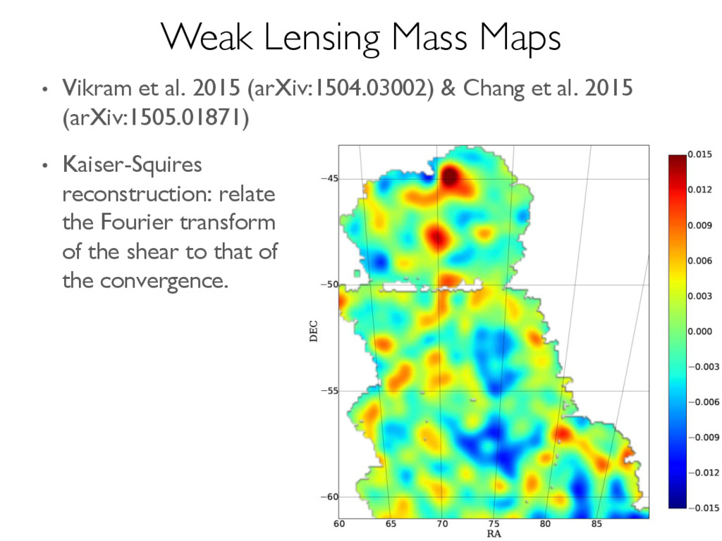
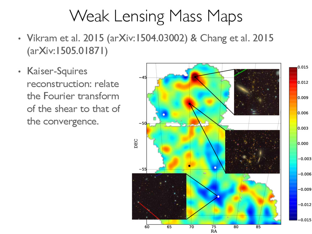
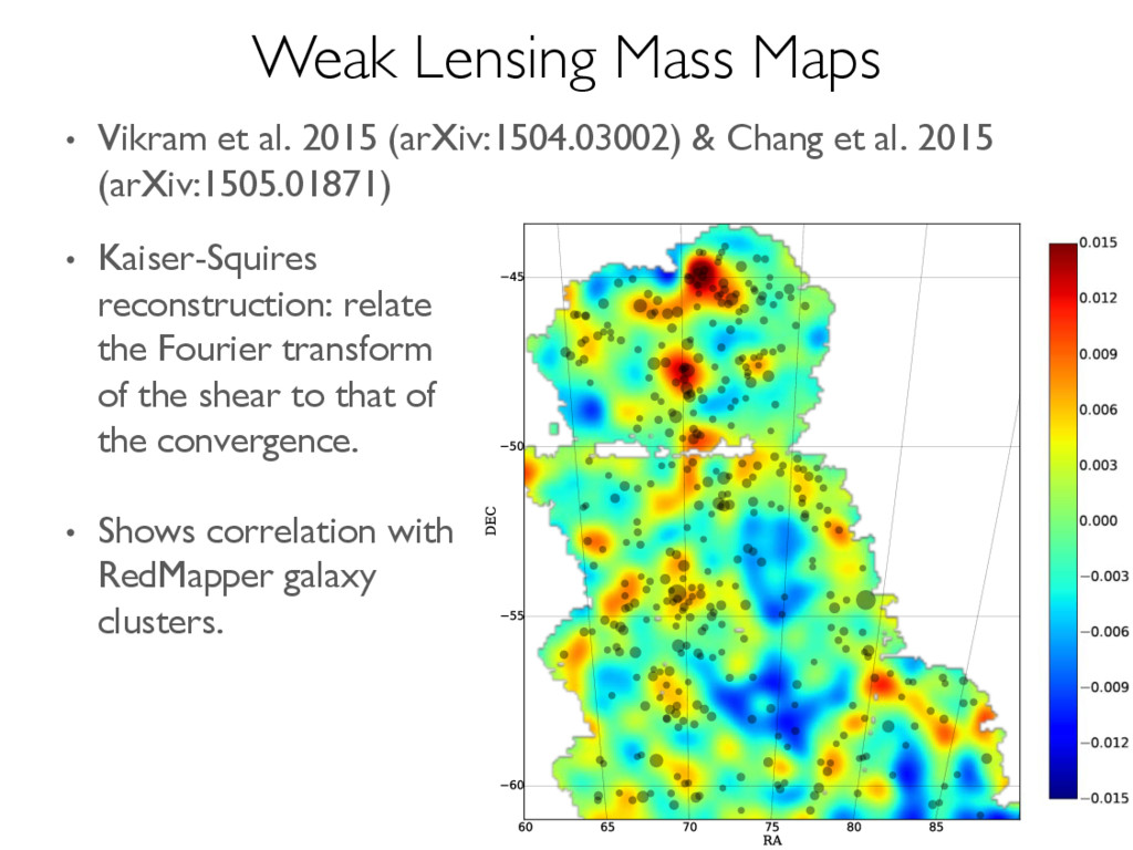
2015 (arXiv:1505.01871) • Kaiser-Squires reconstruction: relate the Fourier transform of the shear to that of the convergence. • Shows correlation with RedMapper galaxy clusters. Weak Lensing Mass Maps
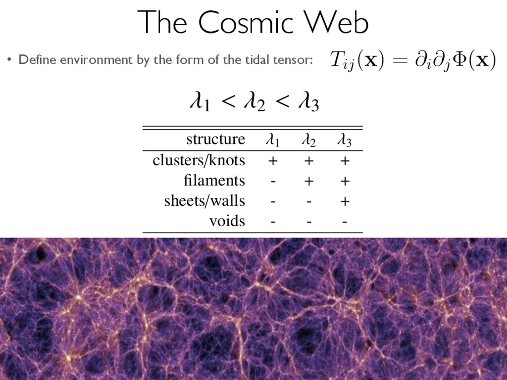
the tidal tensor: structure 1 2 3 clusters/knots + + + filaments - + + sheets/walls - - + voids - - - structure categories defined by the gravitational tidal field tensor, using the ei ns correspond to positive (negative) eigenvalues. e was employed to characterise the alignment of satellites in terms of the c s and projected shapes, with both quantities being accessible also observat in the gravitational field generated by the matter d motion of the test particles; see Equation (12). The fo h directions gravitational forces contract (positive ei ts. For eigenvalues 1 < 2 < 3 , one can thus defin genvector corresponding to 1 specifies the directio also Figure 2). For sheet-like structures, the eigen of the sheet. Clusters, or knots of the cosmic web ons of the tidal tensors, and these ellipsoids tend t ical (see the argument in ? ). Figure 7 shows an exam cult to identify. Candidates for galaxy clusters c on and then be confirmed if redshift information is
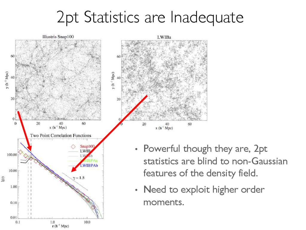
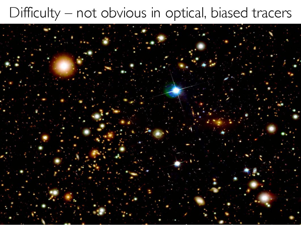
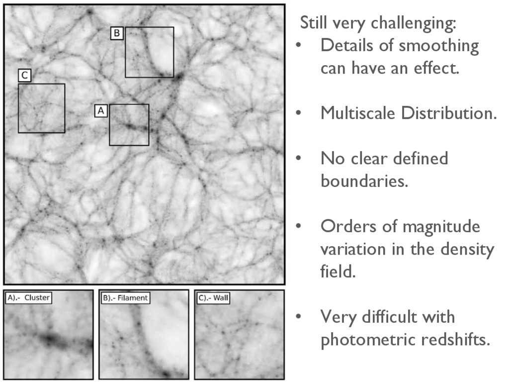
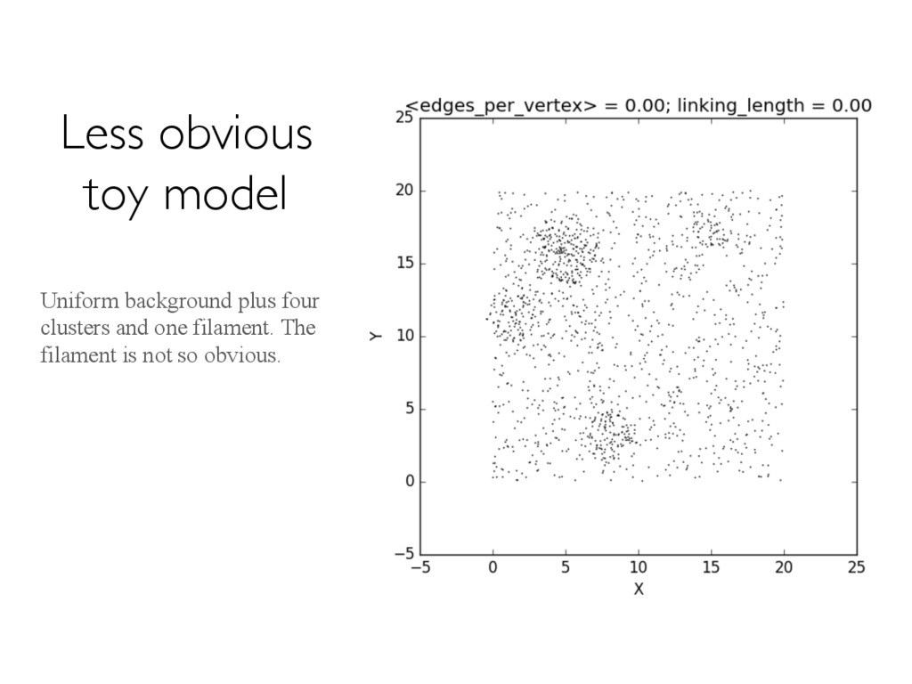
effect. • Multiscale Distribution. • No clear defined boundaries. • Orders of magnitude variation in the density field. • Very difficult with photometric redshifts.
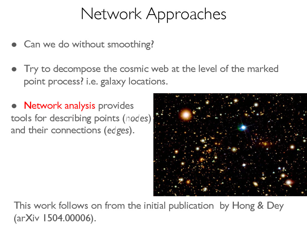
the cosmic web at the level of the marked point process? i.e. galaxy locations. • Network analysis provides tools for describing points (nodes) and their connections (edges). This work follows on from the initial publication by Hong & Dey (arXiv 1504.00006). Network Approaches
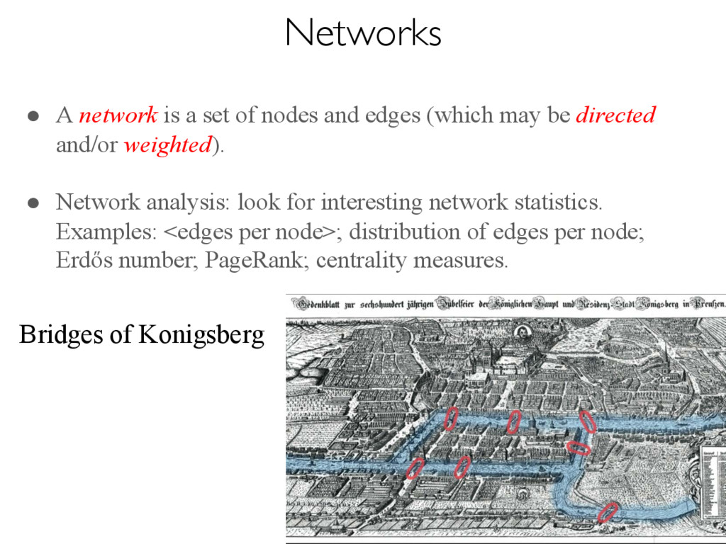
(which may be directed and/or weighted). • Network analysis: look for interesting network statistics. Examples: <edges per node>; distribution of edges per node; Erdős number; PageRank; centrality measures. Bridges of Konigsberg Networks
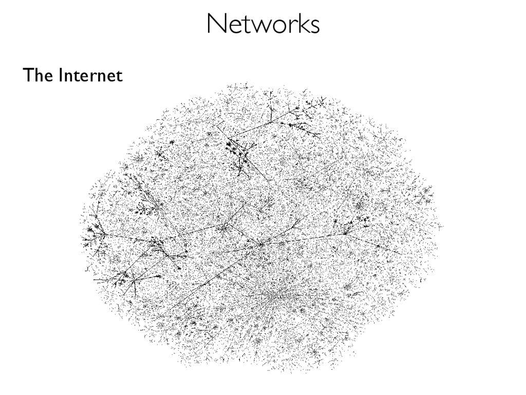
us sys- time of omains, A rout- r tables cture of process revious es. This ors at a f paths gives a nomous ms. As ver the routers dges as P-based n at the measure d from class C nets are tively a nternet, n recent Figure 2.3: The structure of the Internet at the level of autonomous systems. (See Plate III for color version.) The vertices in this netvvork representation of the Internet are autonomous systems and the edges show the routes taken by data traveling between them. This figure is different from Fig. 1.1, which shows the netvvork at the level of class C sub- nets. The picture was created by Hal Burch and Bill Cheswick. Patent(s) pending and Copyright Lumeta Corporation 2009. Reproduced with permission. The Internet Networks
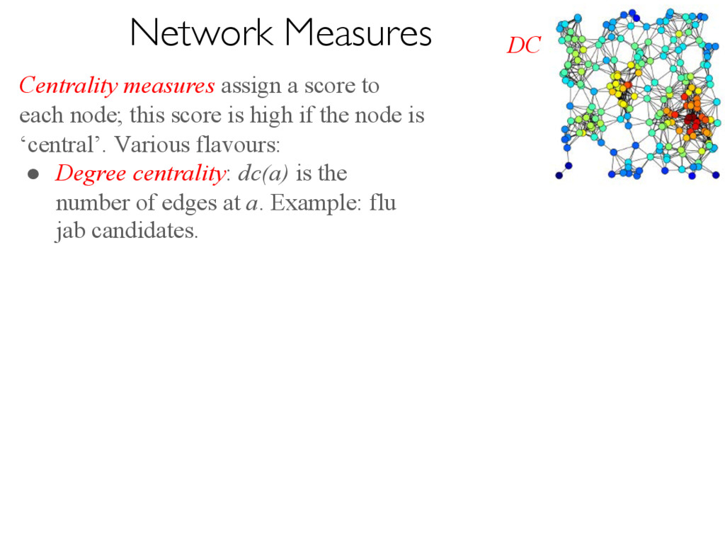
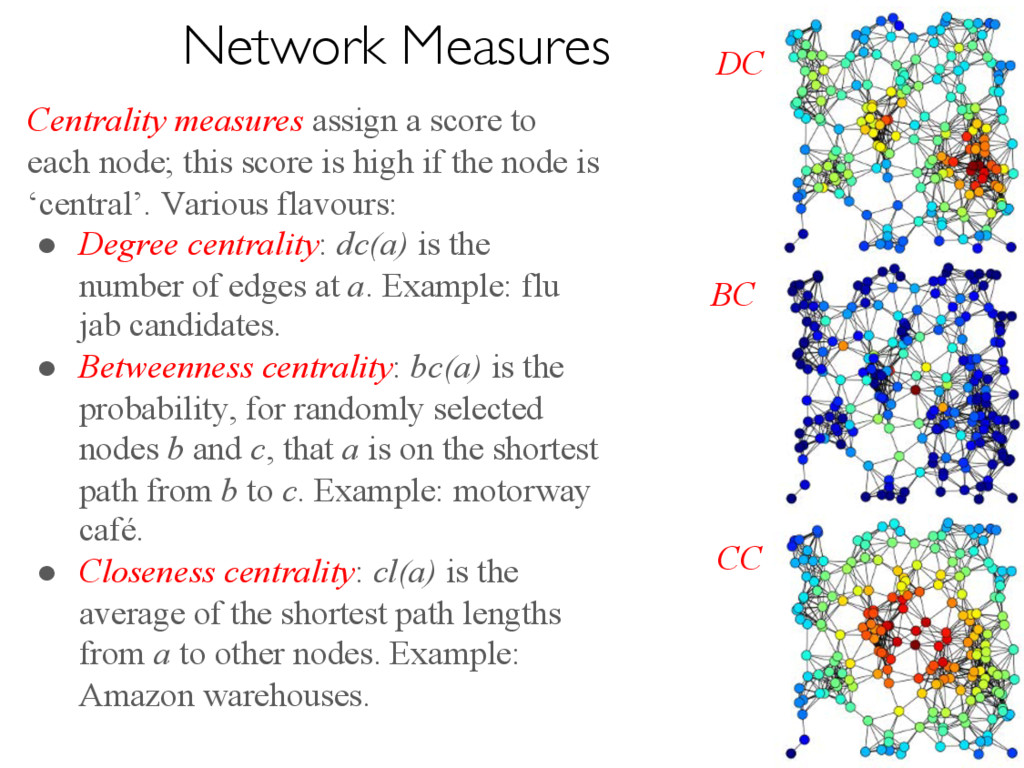
is high if the node is ‘central’. Various flavours: • Degree centrality: dc(a) is the number of edges at a. Example: flu jab candidates. DC Network Measures
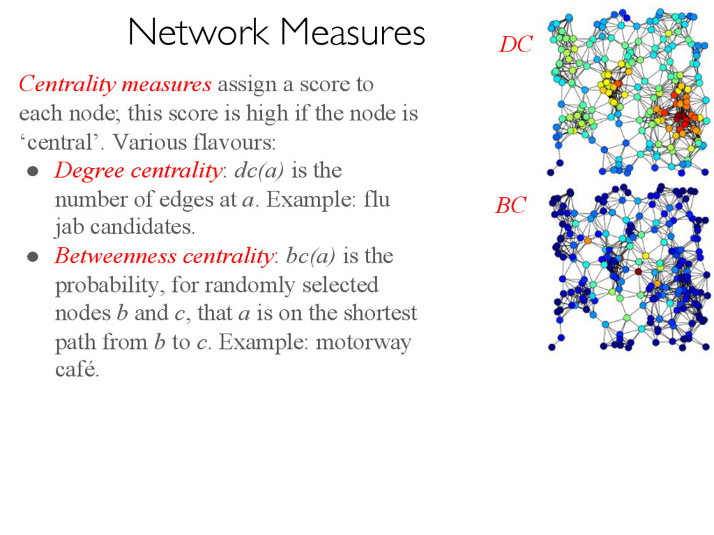
is high if the node is ‘central’. Various flavours: • Degree centrality: dc(a) is the number of edges at a. Example: flu jab candidates. • Betweenness centrality: bc(a) is the probability, for randomly selected nodes b and c, that a is on the shortest path from b to c. Example: motorway café. DC BC Network Measures
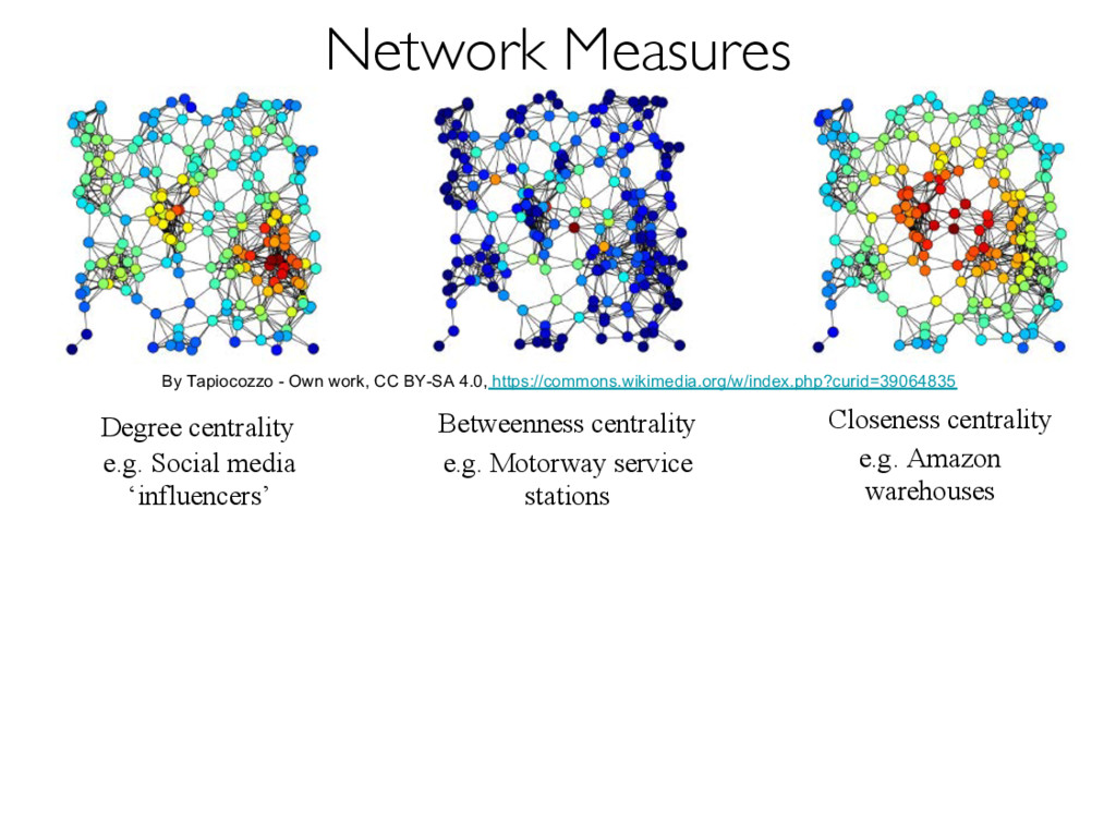
is high if the node is ‘central’. Various flavours: • Degree centrality: dc(a) is the number of edges at a. Example: flu jab candidates. • Betweenness centrality: bc(a) is the probability, for randomly selected nodes b and c, that a is on the shortest path from b to c. Example: motorway café. • Closeness centrality: cl(a) is the average of the shortest path lengths from a to other nodes. Example: Amazon warehouses. DC BC CC Network Measures
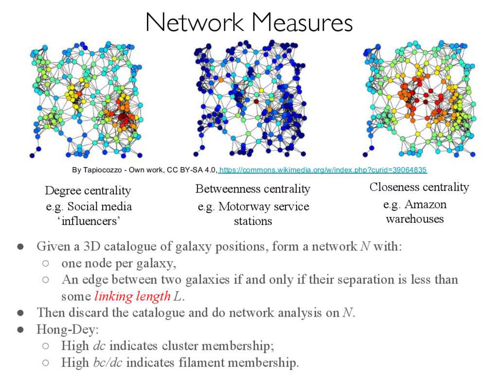
centrality Betweenness centrality Closeness centrality e.g. Social media ‘influencers’ e.g. Motorway service stations e.g. Amazon warehouses Network Measures
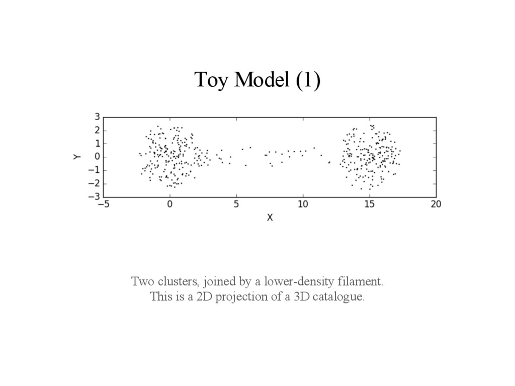
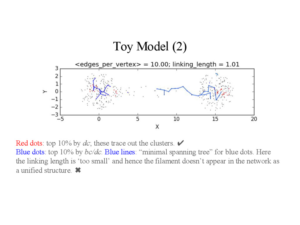
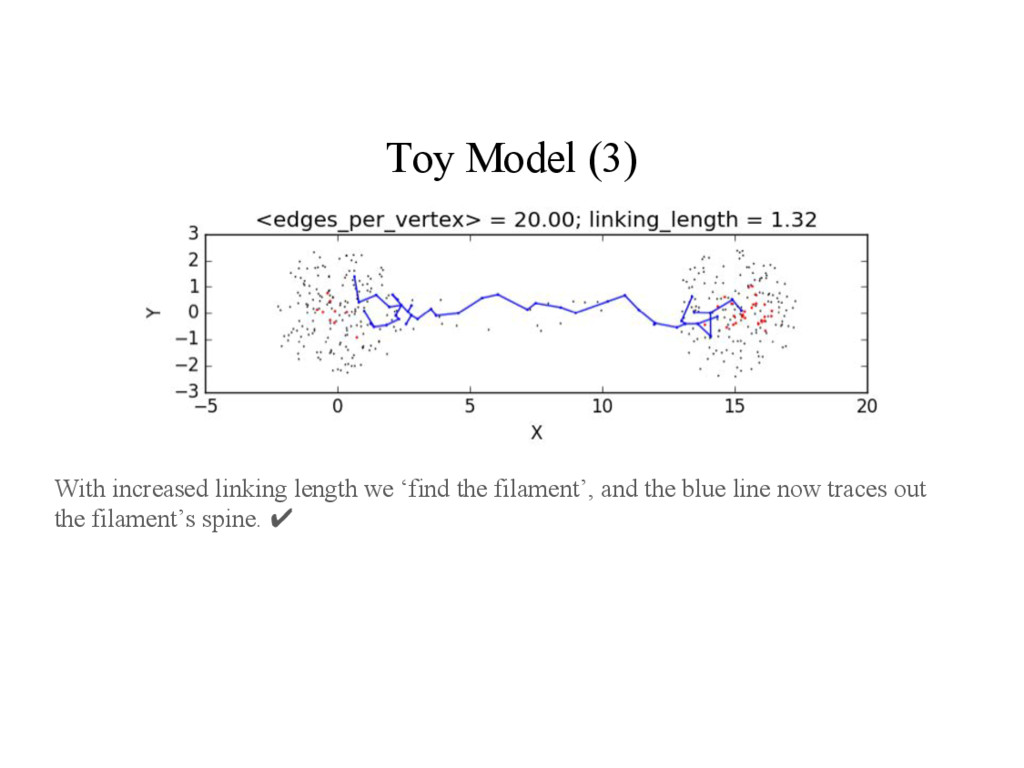
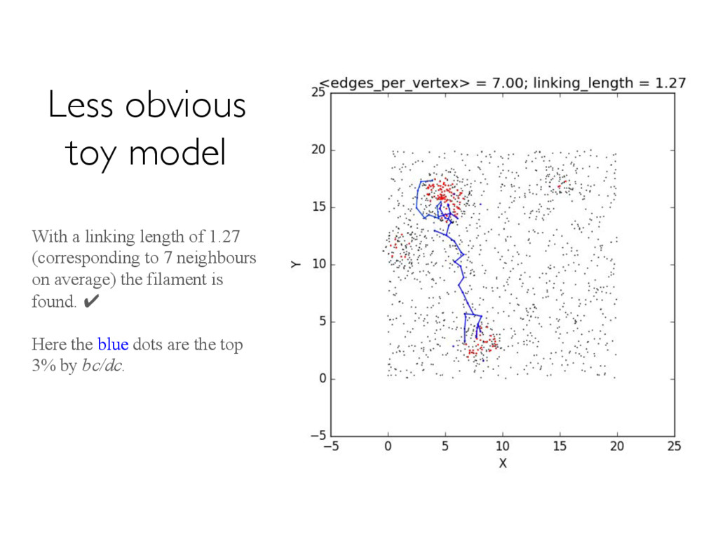
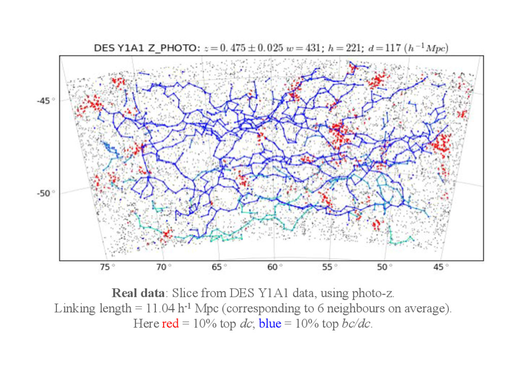
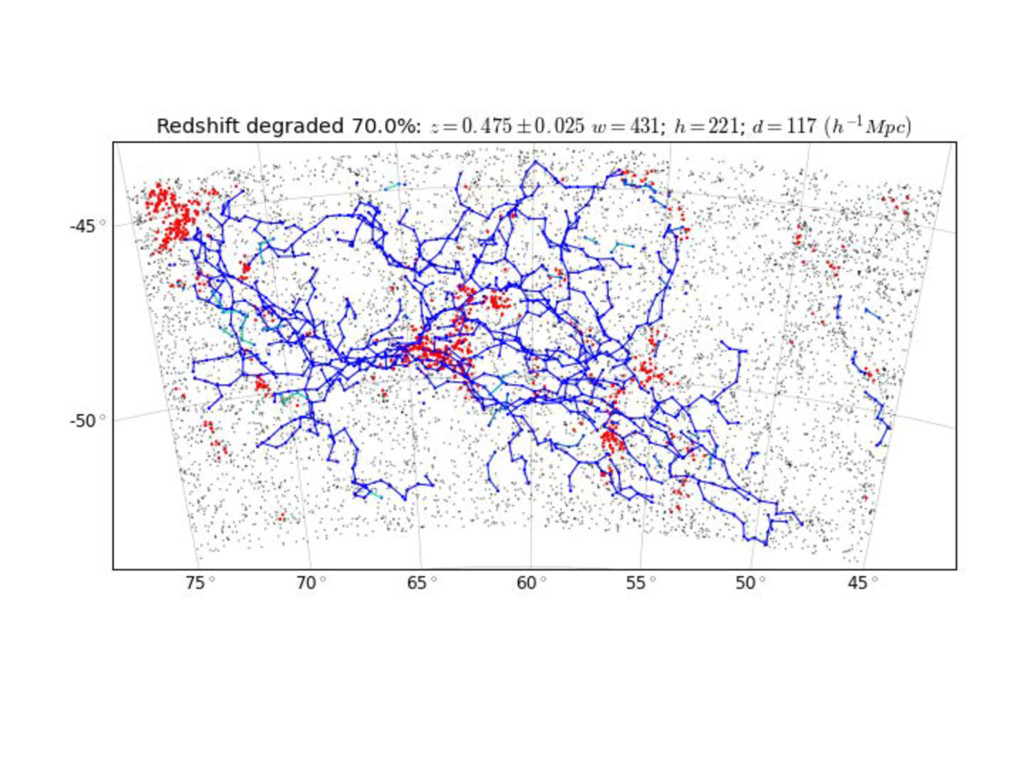
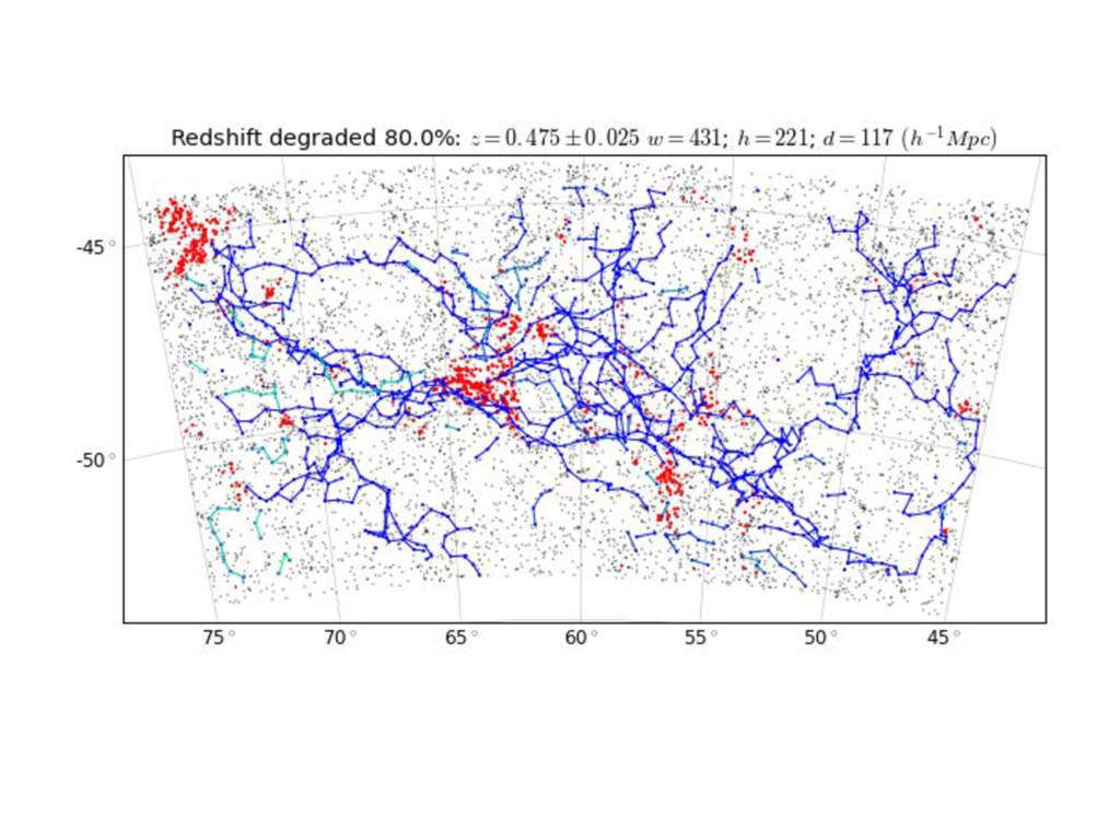
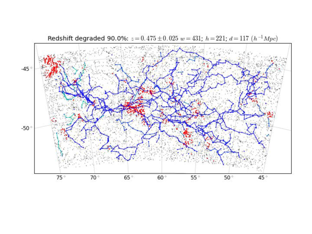
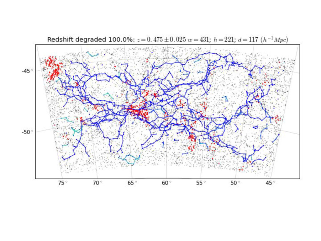
centrality Betweenness centrality Closeness centrality e.g. Social media ‘influencers’ e.g. Motorway service stations e.g. Amazon warehouses • Given a 3D catalogue of galaxy positions, form a network N with: ◦ one node per galaxy, ◦ An edge between two galaxies if and only if their separation is less than some linking length L. • Then discard the catalogue and do network analysis on N. • Hong-Dey: ◦ High dc indicates cluster membership; ◦ High bc/dc indicates filament membership. Network Measures
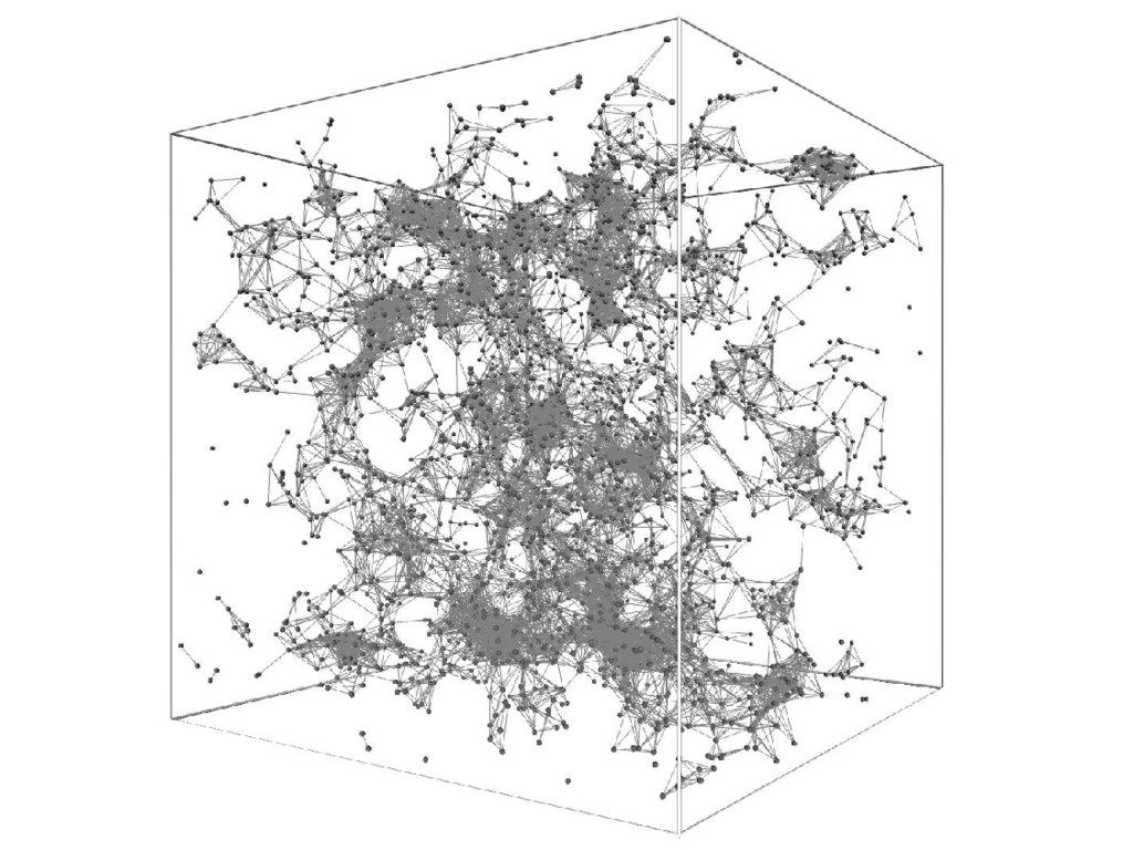
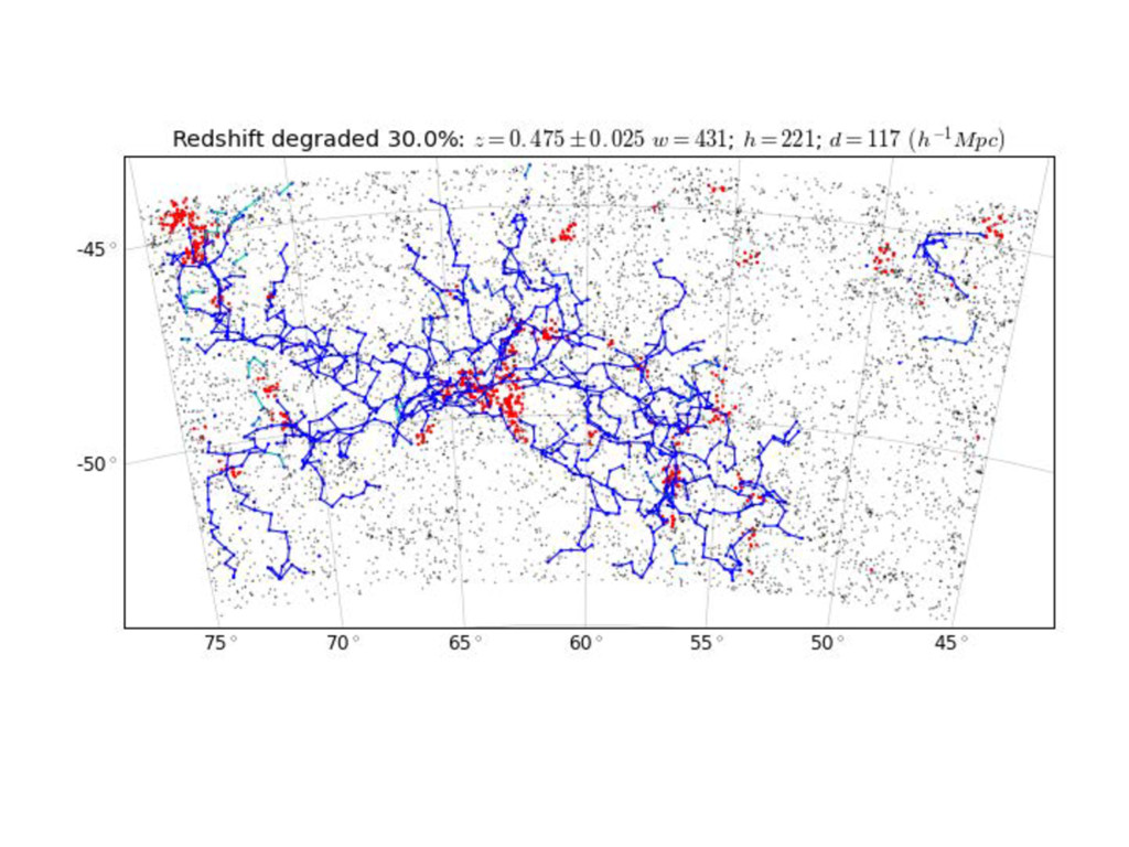
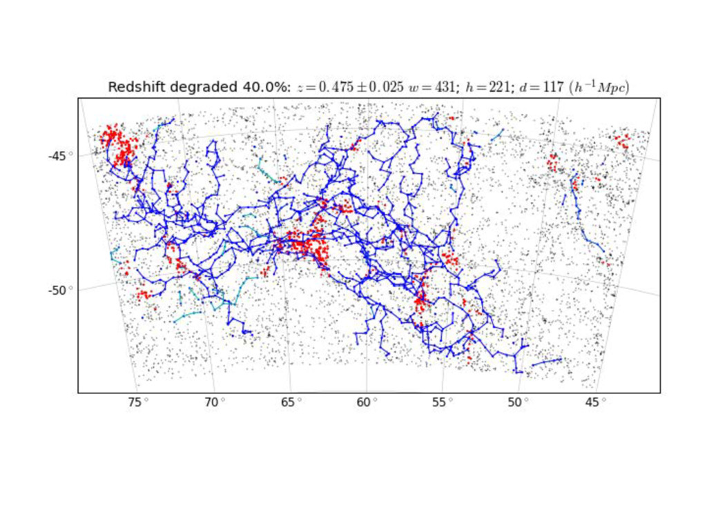
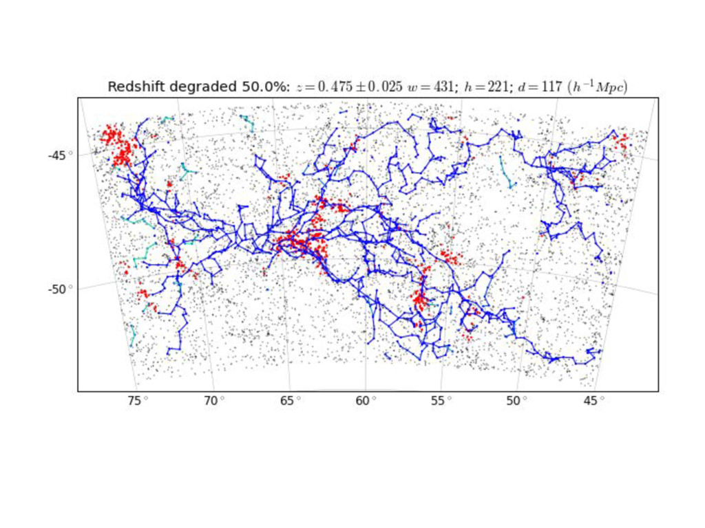
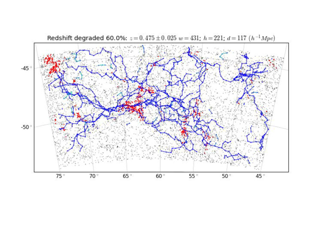
trace out the clusters. ✔ Blue dots: top 10% by bc/dc. Blue lines: “minimal spanning tree” for blue dots. Here the linking length is ‘too small’ and hence the filament doesn’t appear in the network as a unified structure. ✖
colour, morphology, velocity… • A more fundamentally probabilistic method would be nice. • Need to understand quantitively and qualitatively how the method deals with masks. • Most of all: how do we know our result is in any way meaningful?
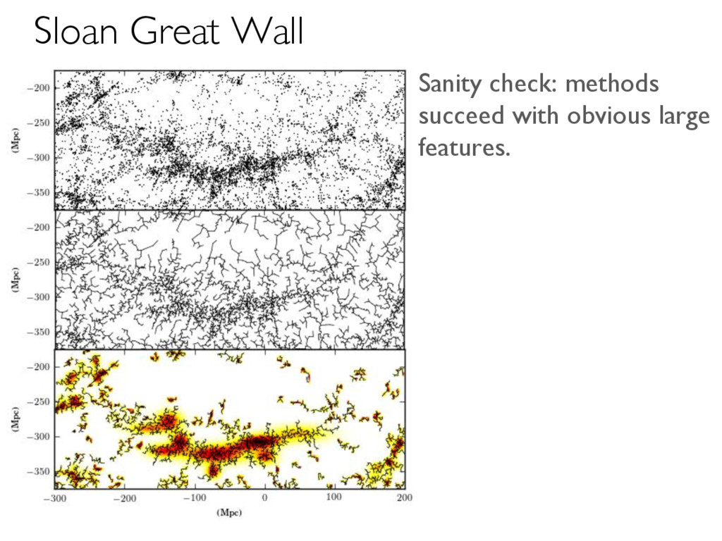
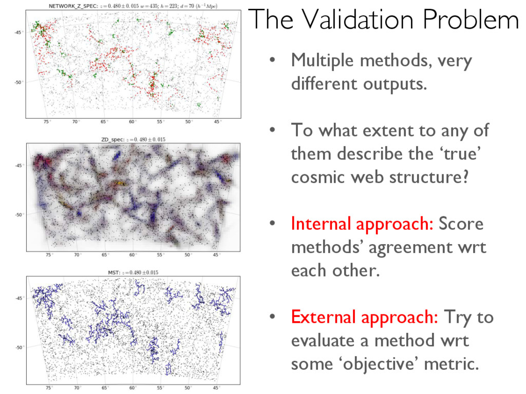
to any of them describe the ‘true’ cosmic web structure? • Internal approach: Score methods’ agreement wrt each other. • External approach: Try to evaluate a method wrt some ‘objective’ metric. The Validation Problem
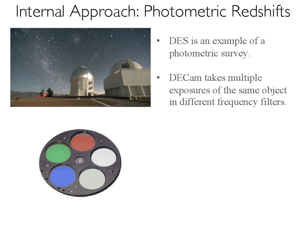
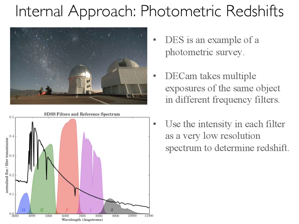
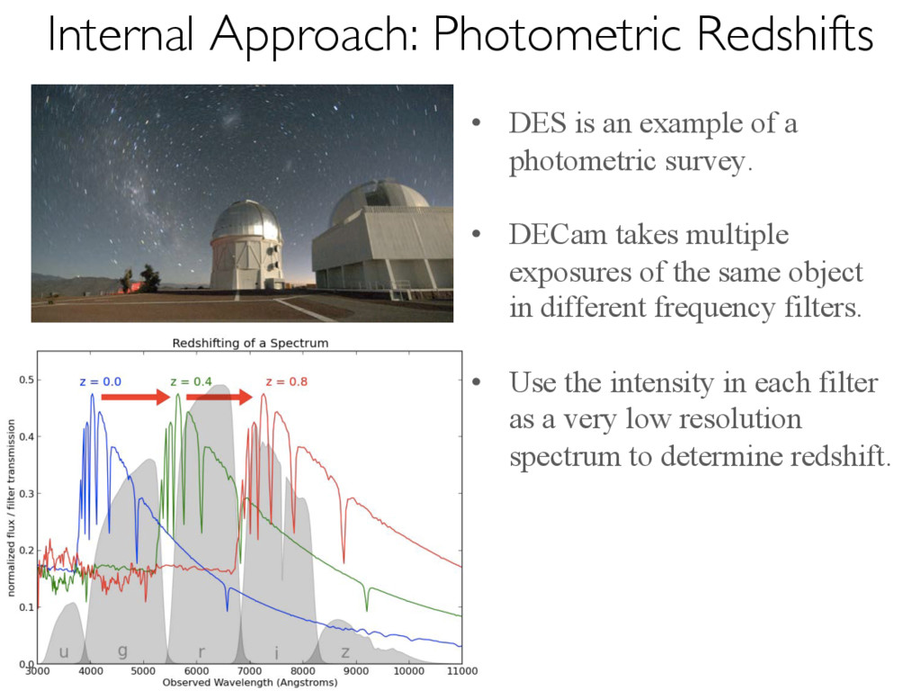
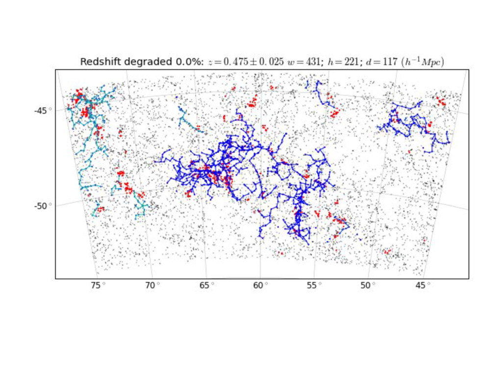
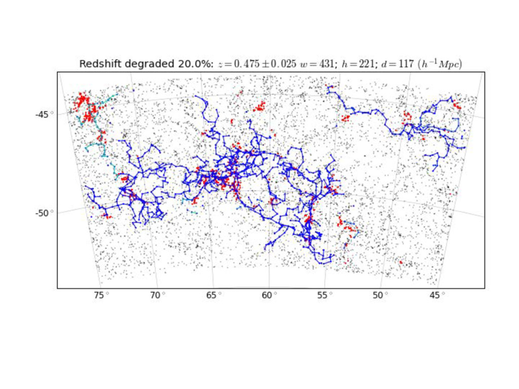
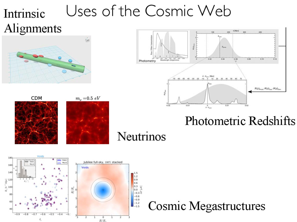
DECam takes multiple exposures of the same object in different frequency filters. • Use the intensity in each filter as a very low resolution spectrum to determine redshift. Internal Approach: Photometric Redshifts
DECam takes multiple exposures of the same object in different frequency filters. • Use the intensity in each filter as a very low resolution spectrum to determine redshift. Internal Approach: Photometric Redshifts
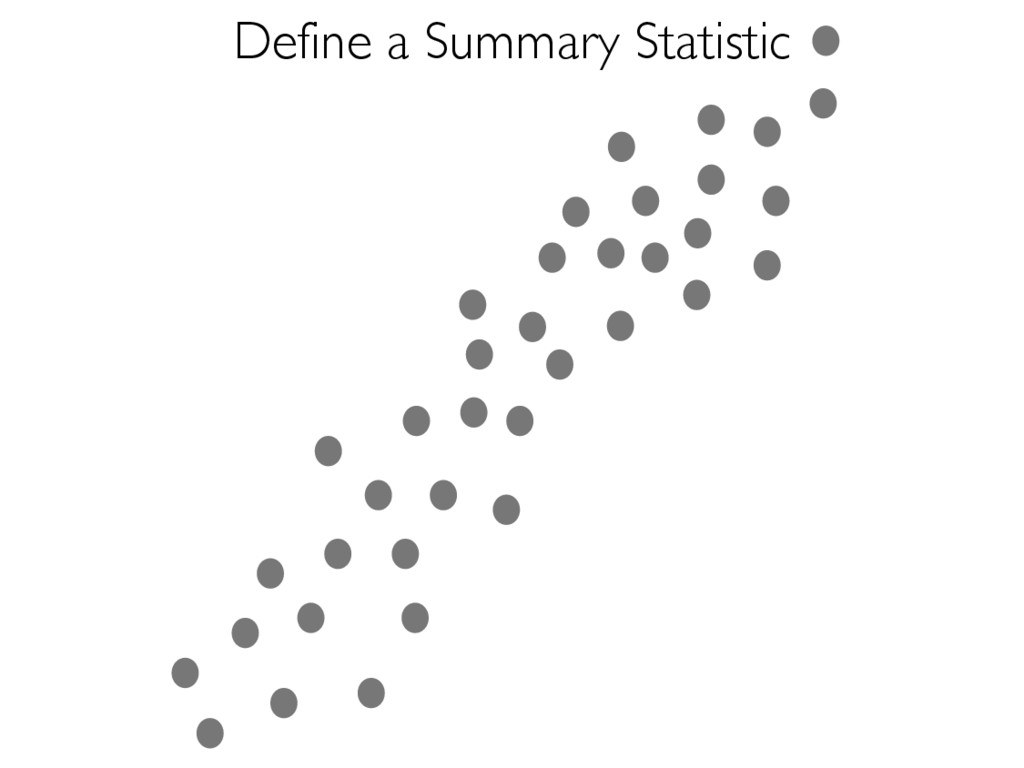
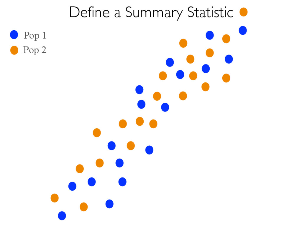
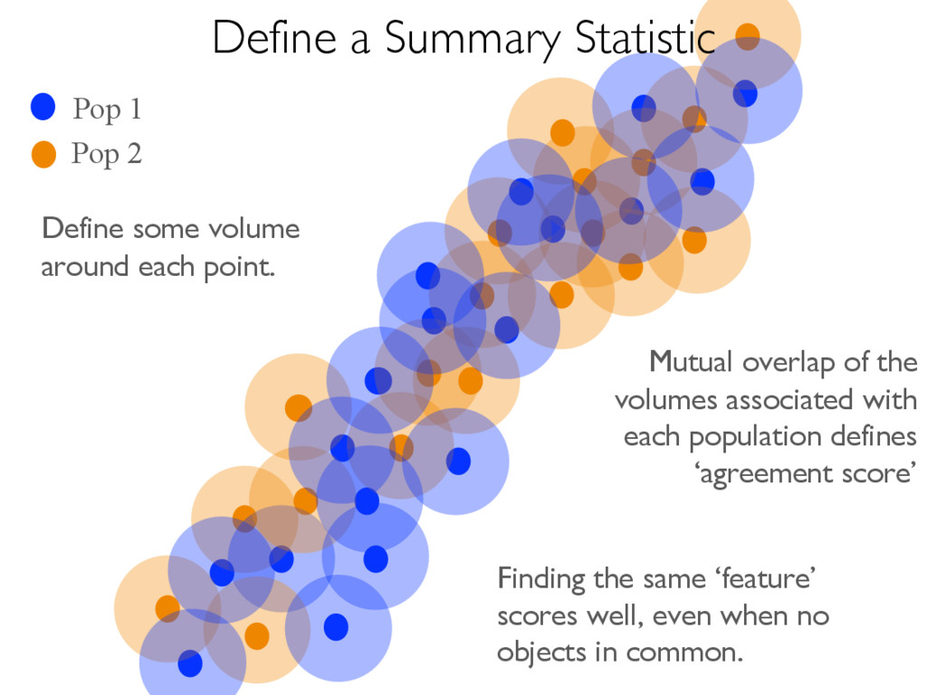
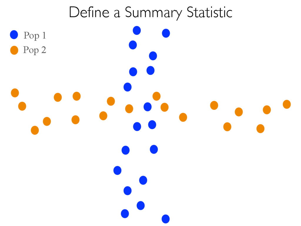
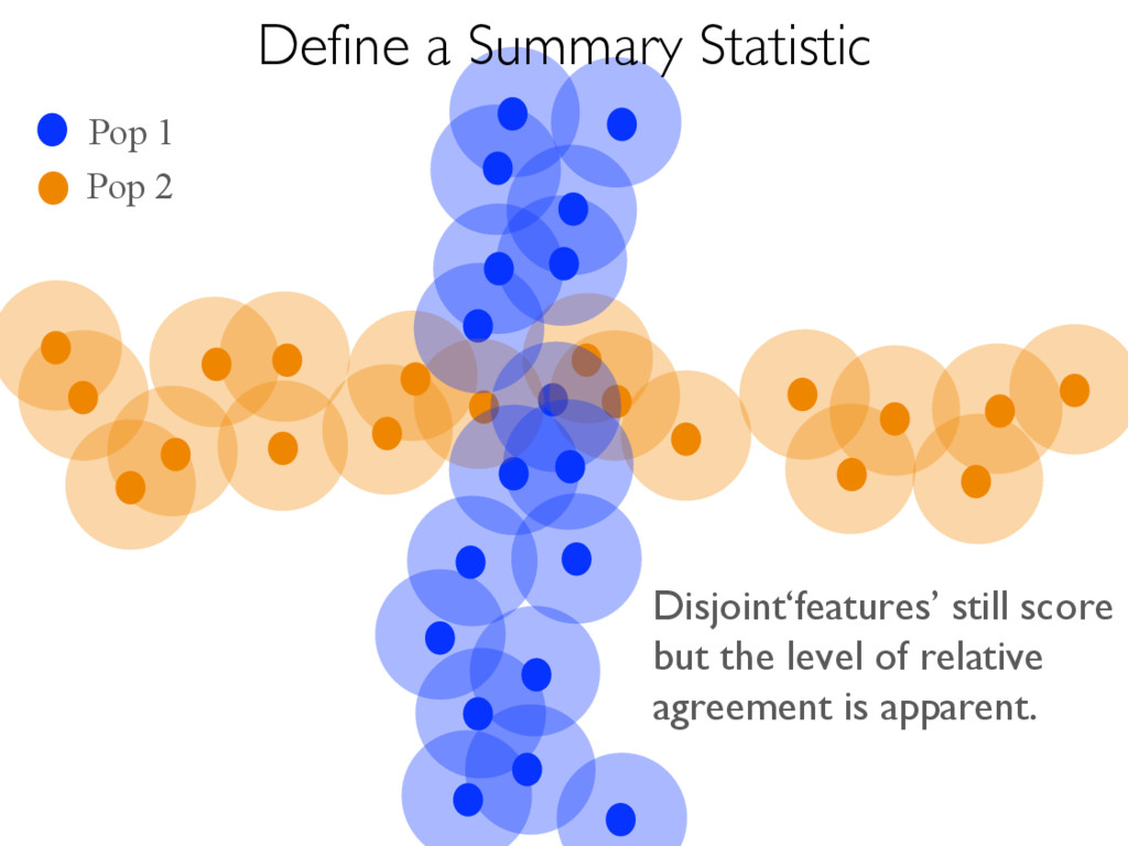
Mutual overlap of the volumes associated with each population defines ‘agreement score’ Finding the same ‘feature’ scores well, even when no objects in common. Define a Summary Statistic
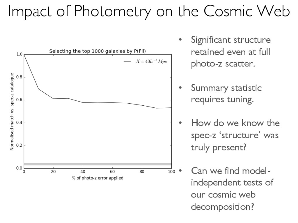
retained even at full photo-z scatter. • Summary statistic requires tuning. • How do we know the spec-z ‘structure’ was truly present? • Can we find model- independent tests of our cosmic web decomposition?