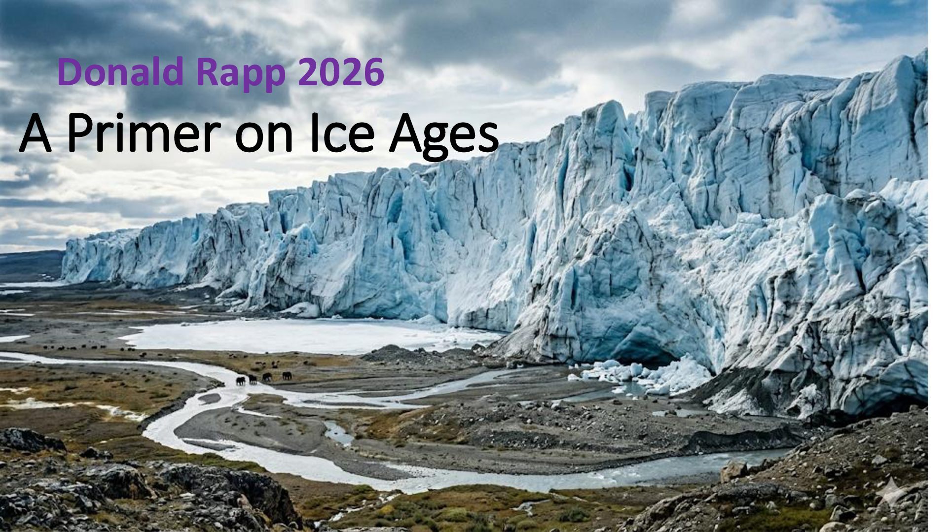
A 64-slide review of all aspects of Ice Ages including description, ice cores, ocean sediments, review and graphical summary of known results, models based on solar variations due to orbital variations.
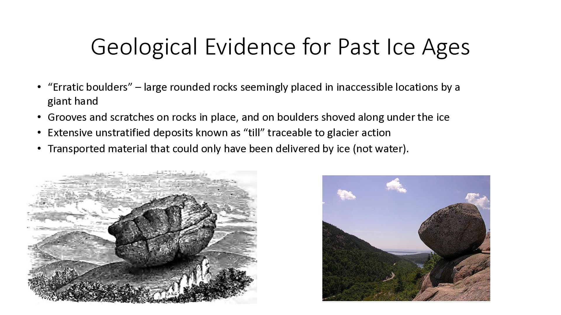
large rounded rocks seemingly placed in inaccessible locations by a giant hand • Grooves and scratches on rocks in place, and on boulders shoved along under the ice • Extensive unstratified deposits known as “till” traceable to glacier action • Transported material that could only have been delivered by ice (not water).
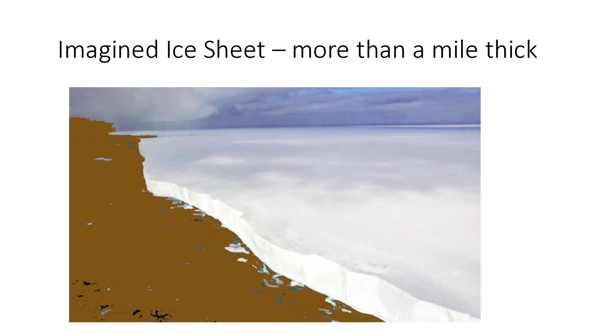
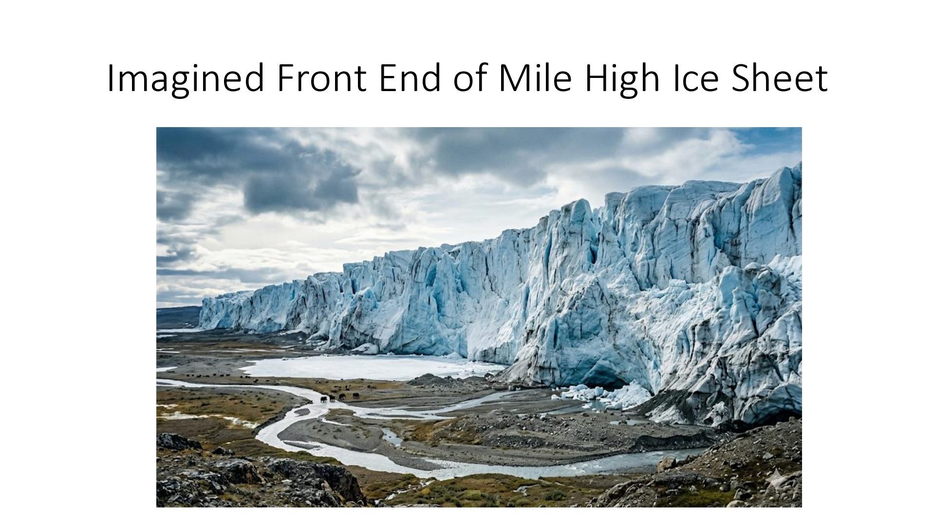
discovered that: • Over the past 3 million years, the Earth has undergone roughly 60 major ice age cycles • Spaced at 41,000 to 110,000 years, with interglacial periods separating ice accumulation periods • Each ice age involves transfer of several percent of the water in the oceans to gigantic ice sheets in the Northern Hemisphere • In an ice age, large portions of Canada, Siberia and Scandinavia remain under ice and snow year-round covered by ice sheets more than a mile thick • The most recent ice age peaked around a mere 20,000 years ago and terminated over the period from 18,000 years ago to about 8,000 years ago
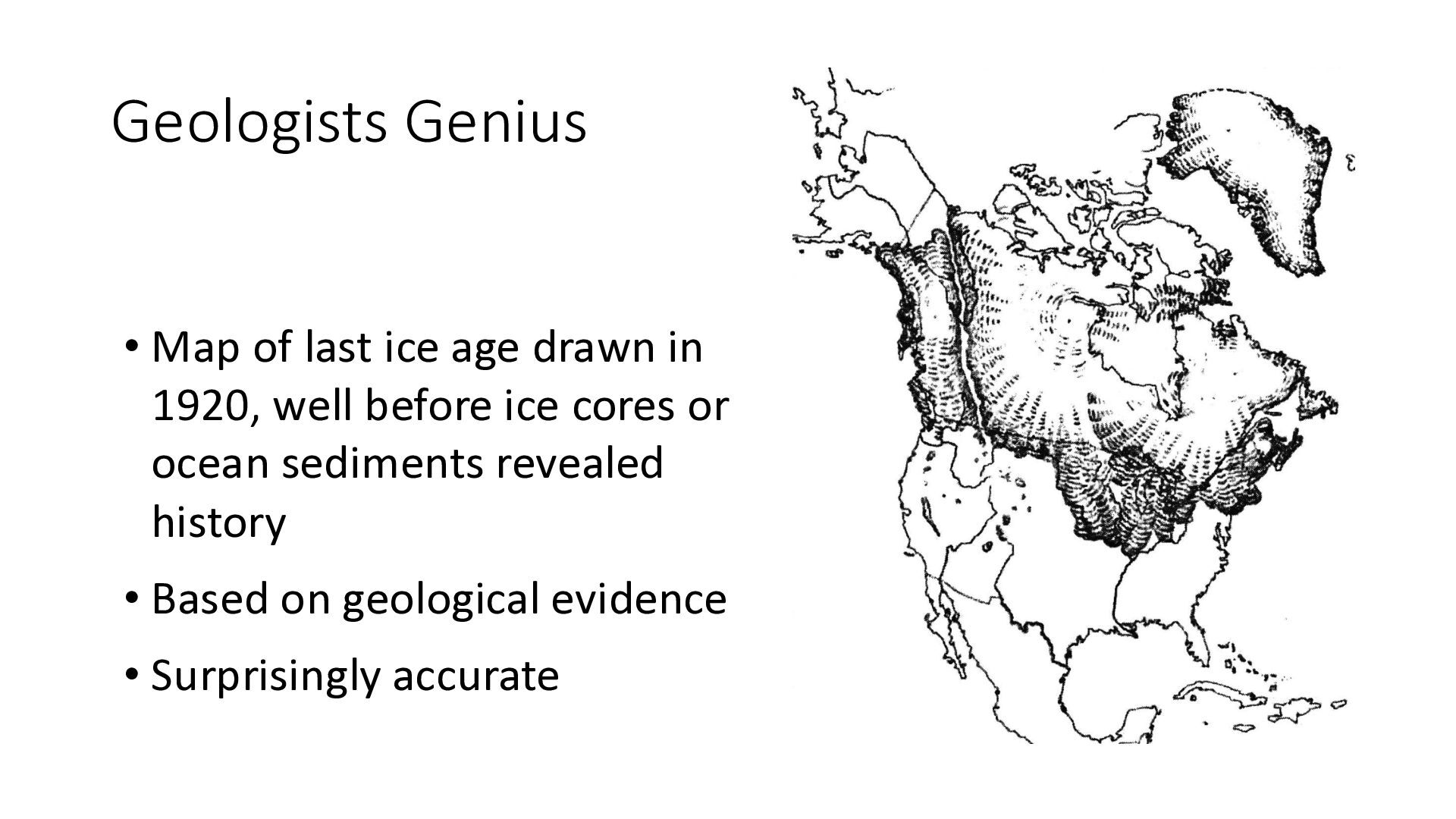
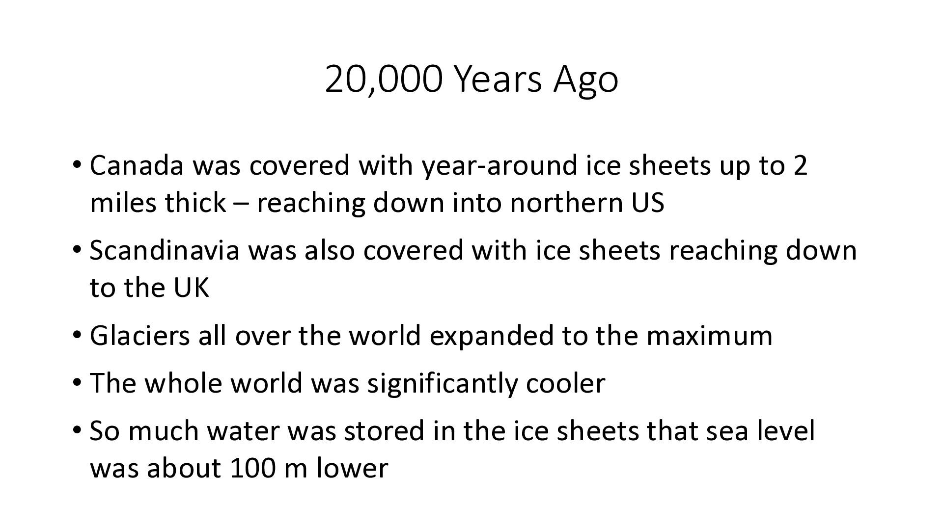
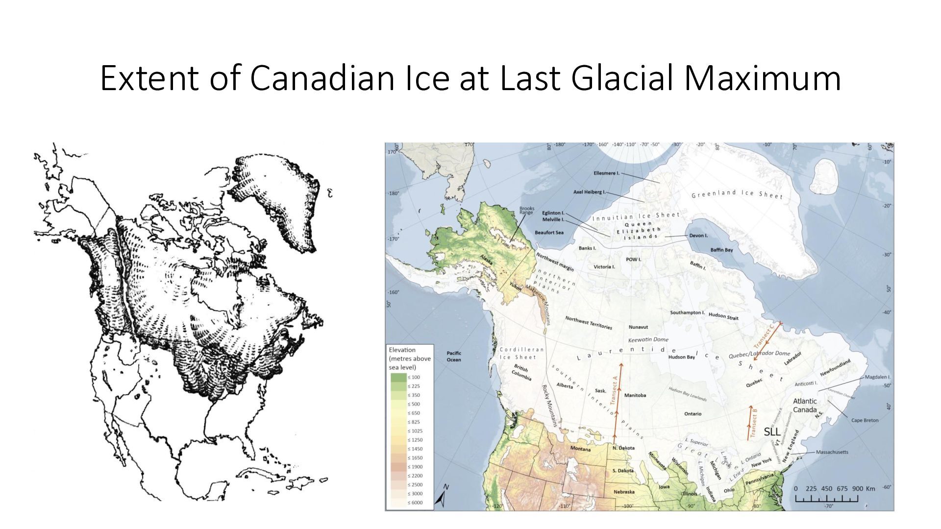
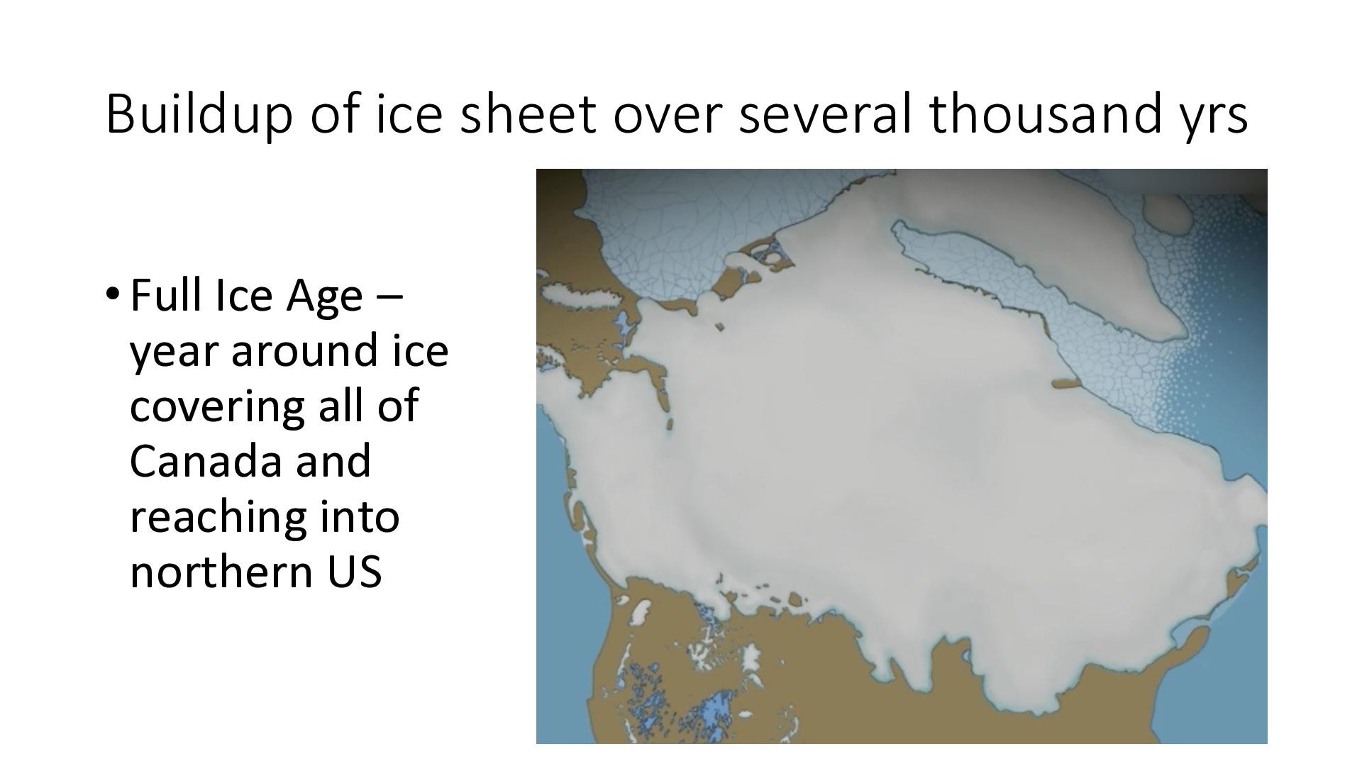
sheets up to 2 miles thick – reaching down into northern US • Scandinavia was also covered with ice sheets reaching down to the UK • Glaciers all over the world expanded to the maximum • The whole world was significantly cooler • So much water was stored in the ice sheets that sea level was about 100 m lower
in the broad swath of Canada, winter snow accumulates in winter • But across most of Canada, the snow melts annually in summer due to the solar input of energy • During an ice age, the solar input is unable to melt all the snow/ice in summer and the snowpack accumulates • As time passes, the snow turns to ice and an ice sheet forms • Evidently, to understand ice ages, we need to understand the variability of “solar input to high northern latitudes” (SIHNL)
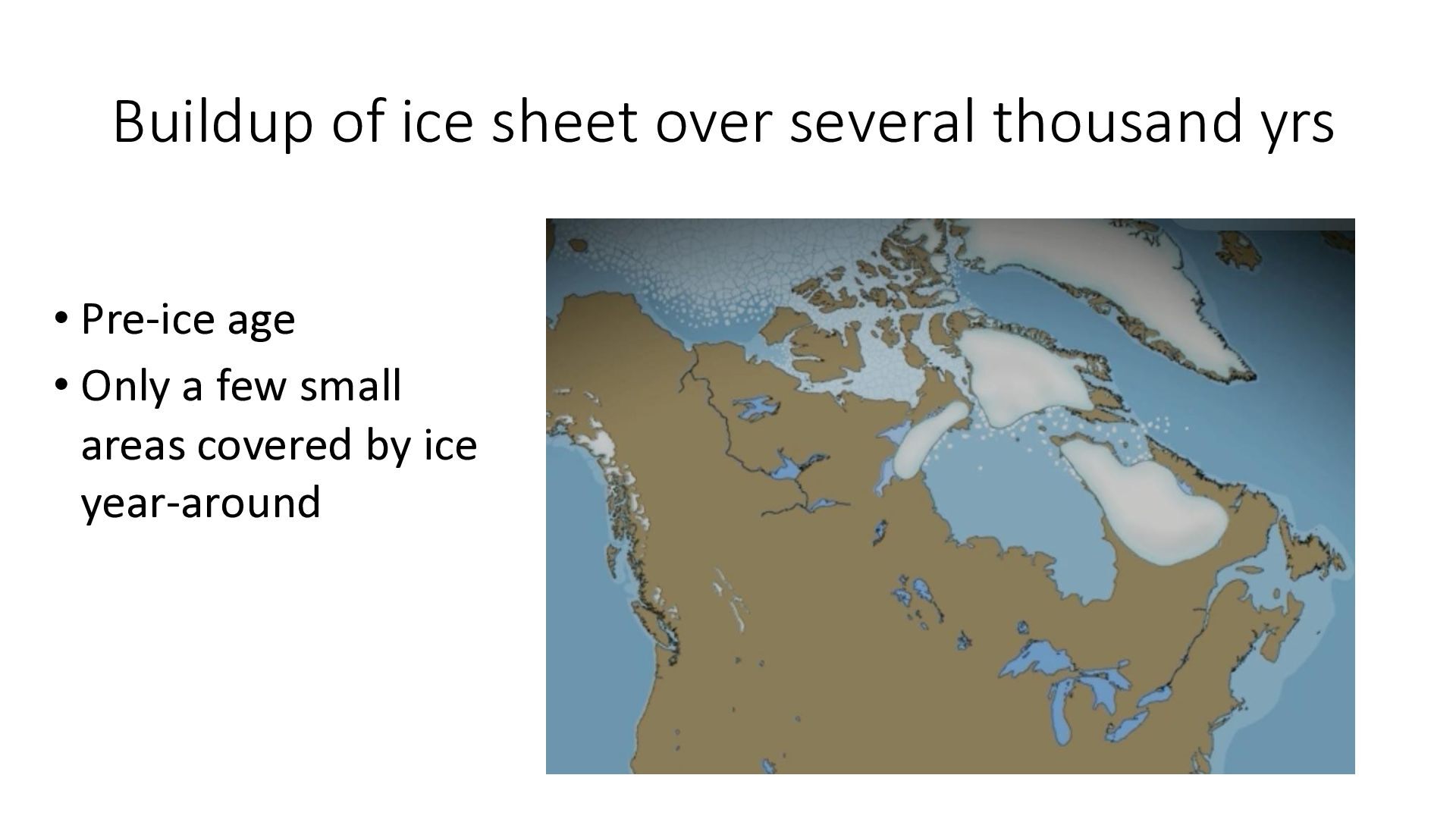
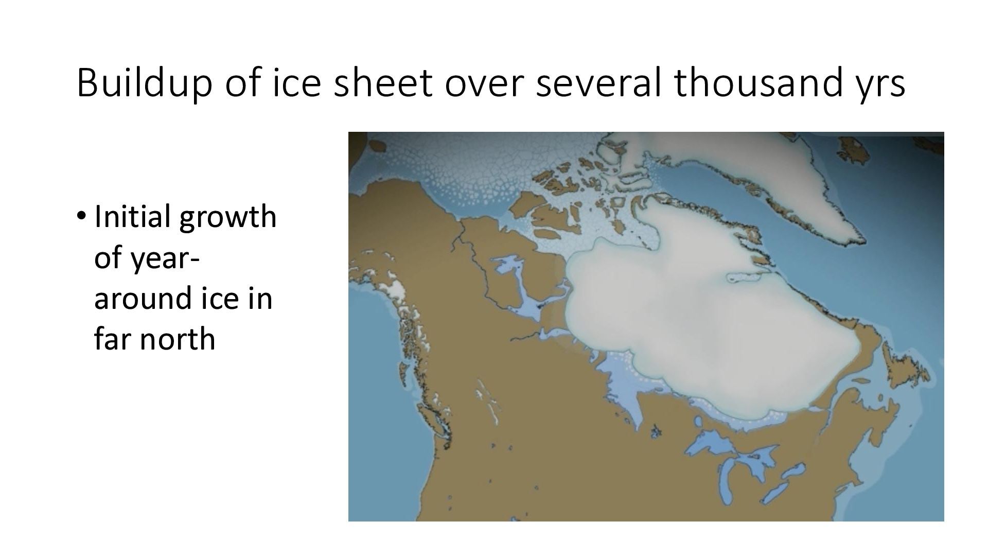
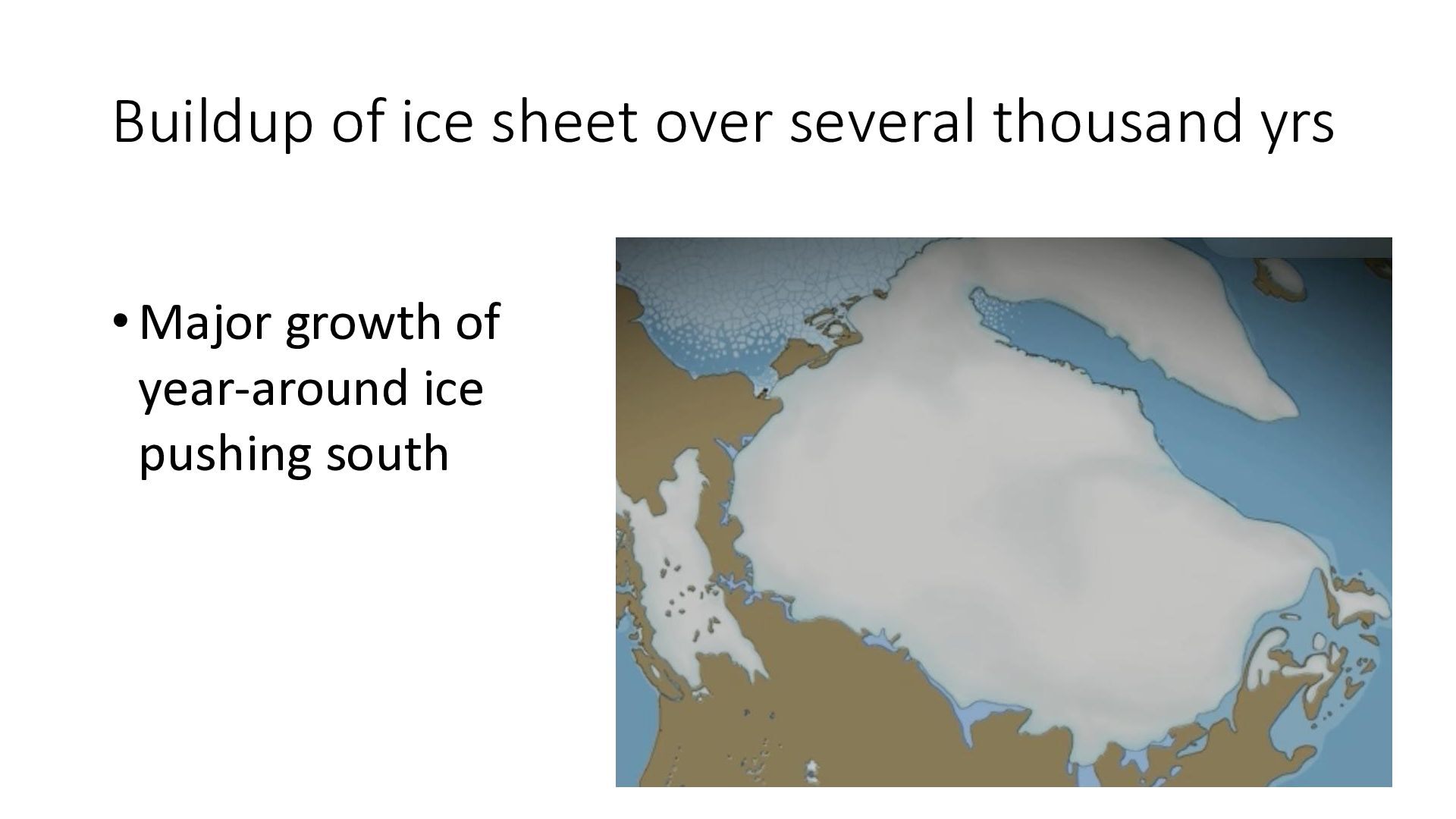
early stages of an ice age, small parts of northern Canada that used to be ice free in summer begin to ice over year-around • As hundreds of years pass, more and more area is covered by year-round ice, moving southward from the north • After 5,000 to 8,000 years, essentially all of Canada is covered by year-around ice • After that, the ice continues to thicken over many years • When termination begins, small pockets of ice melt during summer • As hundreds of years pass, more and more area has summer melt moving northward • After 5,000 to 8,000 years, winter ice melts in summer across Canada
(warm) period, • Moderate surface ice and snow covers most of Canada in winter • Surface ice and snow melts across most of Canada during summer • In a glacial period, • Thick surface ice and snow covers most of Canada in winter • Surface ice and snow remains mainly un-melted across most of Canada during summer • The difference between glacial and interglacial periods must be the heat input to the surface during summer – determines whether winter ice/snow survives the summer • The obvious source of a difference between heat input to surface ice/snow from year to year has to be changes in solar input from year to year
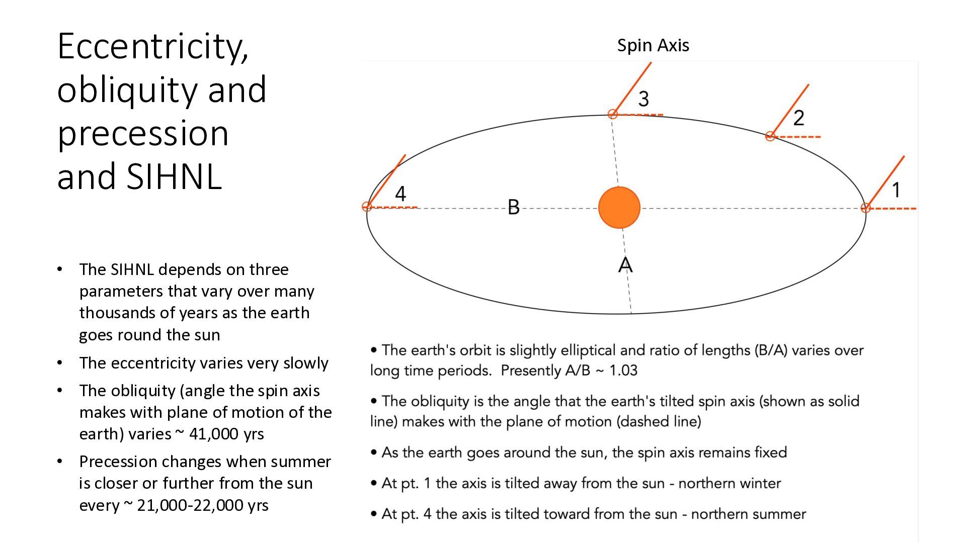
many thousands of years: • Changes in the slightly elliptical orbit of the earth around the sun • Changes in the tilt angle the earth’s axis makes with it plane of motion • Changes in the tilt angle itself • Produce quasi-periodic changes in SIHNL
on three parameters that vary over many thousands of years as the earth goes round the sun • The eccentricity varies very slowly • The obliquity (angle the spin axis makes with plane of motion of the earth) varies ~ 41,000 yrs • Precession changes when summer is closer or further from the sun every ~ 21,000-22,000 yrs Spin Axis
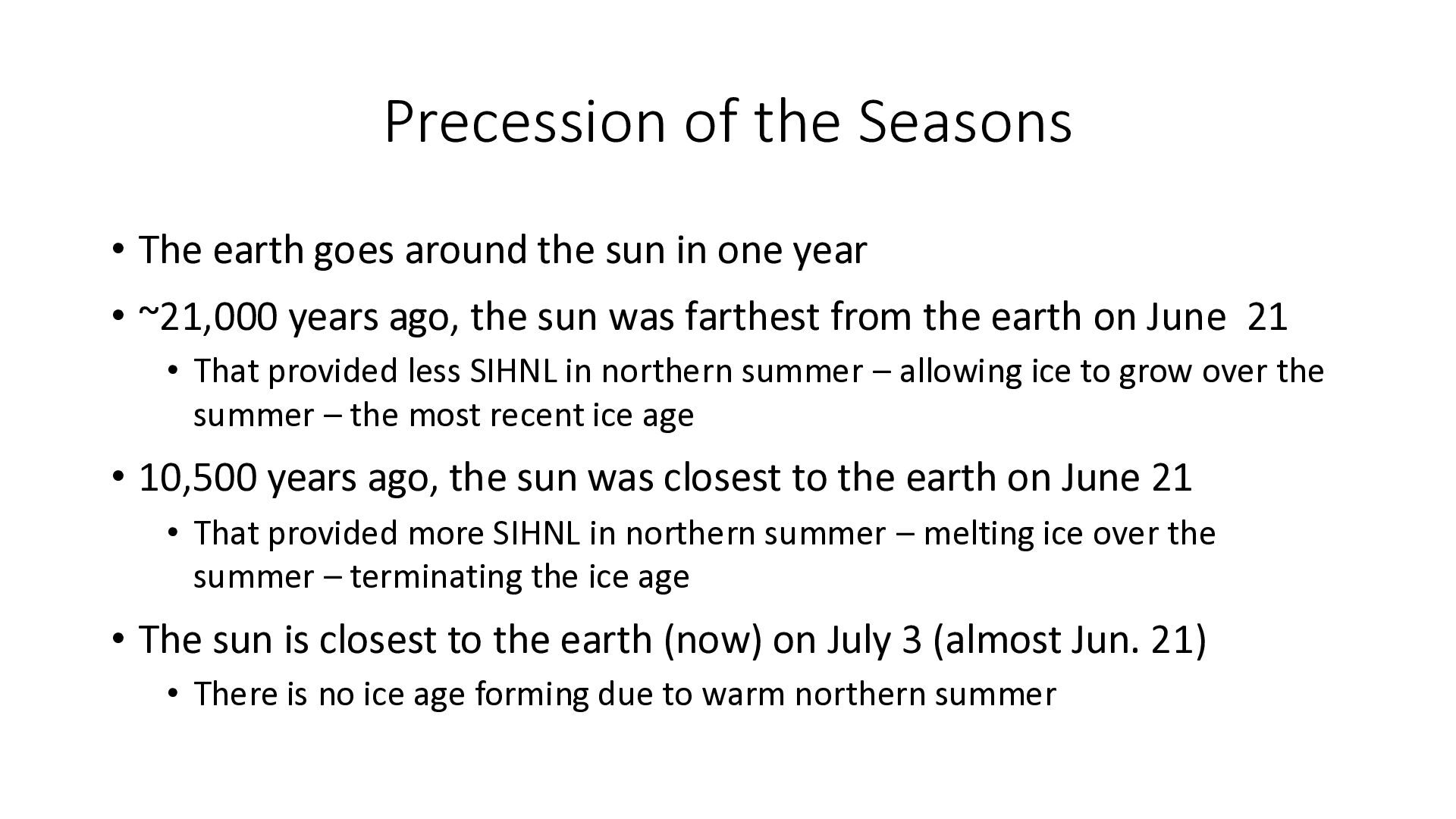
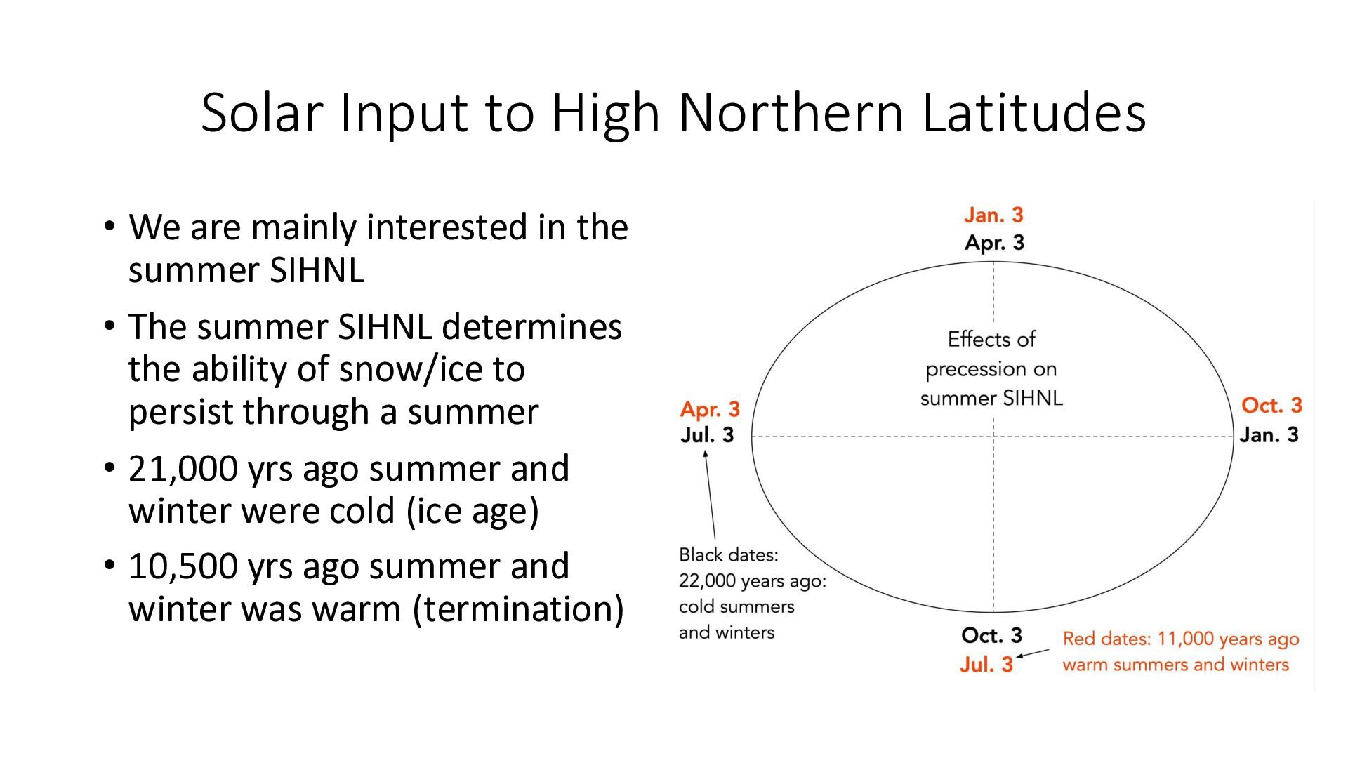
sun in one year • ~21,000 years ago, the sun was farthest from the earth on June 21 • That provided less SIHNL in northern summer – allowing ice to grow over the summer – the most recent ice age • 10,500 years ago, the sun was closest to the earth on June 21 • That provided more SIHNL in northern summer – melting ice over the summer – terminating the ice age • The sun is closest to the earth (now) on July 3 (almost Jun. 21) • There is no ice age forming due to warm northern summer
interested in the summer SIHNL • The summer SIHNL determines the ability of snow/ice to persist through a summer • 21,000 yrs ago summer and winter were cold (ice age) • 10,500 yrs ago summer and winter was warm (termination)
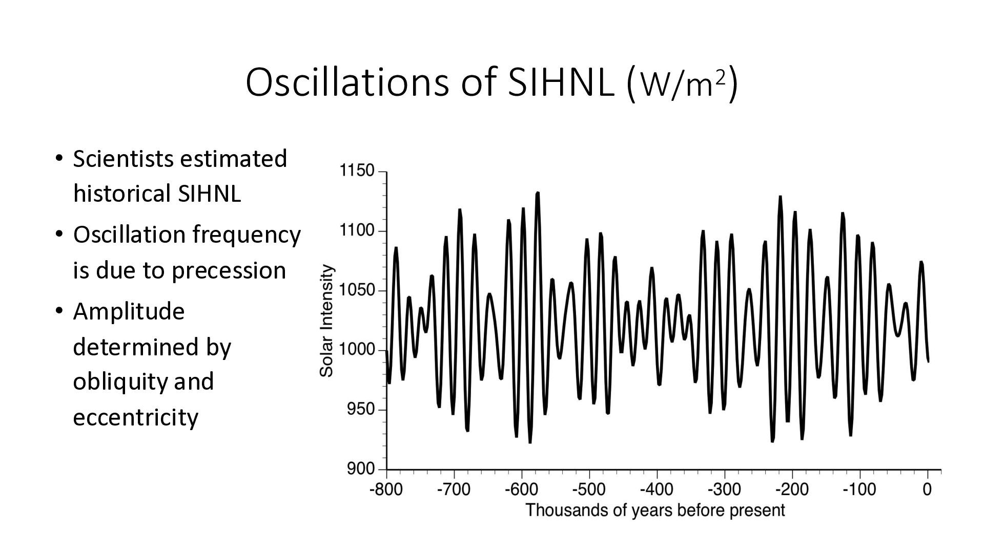
years • The earth moves in a plane in a slightly elliptical orbit • Three parameters vary with time: • The tilt of the earth (obliquity) relative to its plane of motion varies with a period of roughly 41,000 years • The eccentricity of the elliptical orbit varies with a period ranging near 100,000 years • The season when the earth is closest to the sun varies (“precession”) with a period of roughly 21,000 to 22,000 years • These changes in the earth’s orbit and tilt cause the SIHNL to vary over long time periods • The primary factor is precession, producing a 22,000-year oscillation in SIHNL, but eccentricity and obliquity affect the amplitude of the oscillation
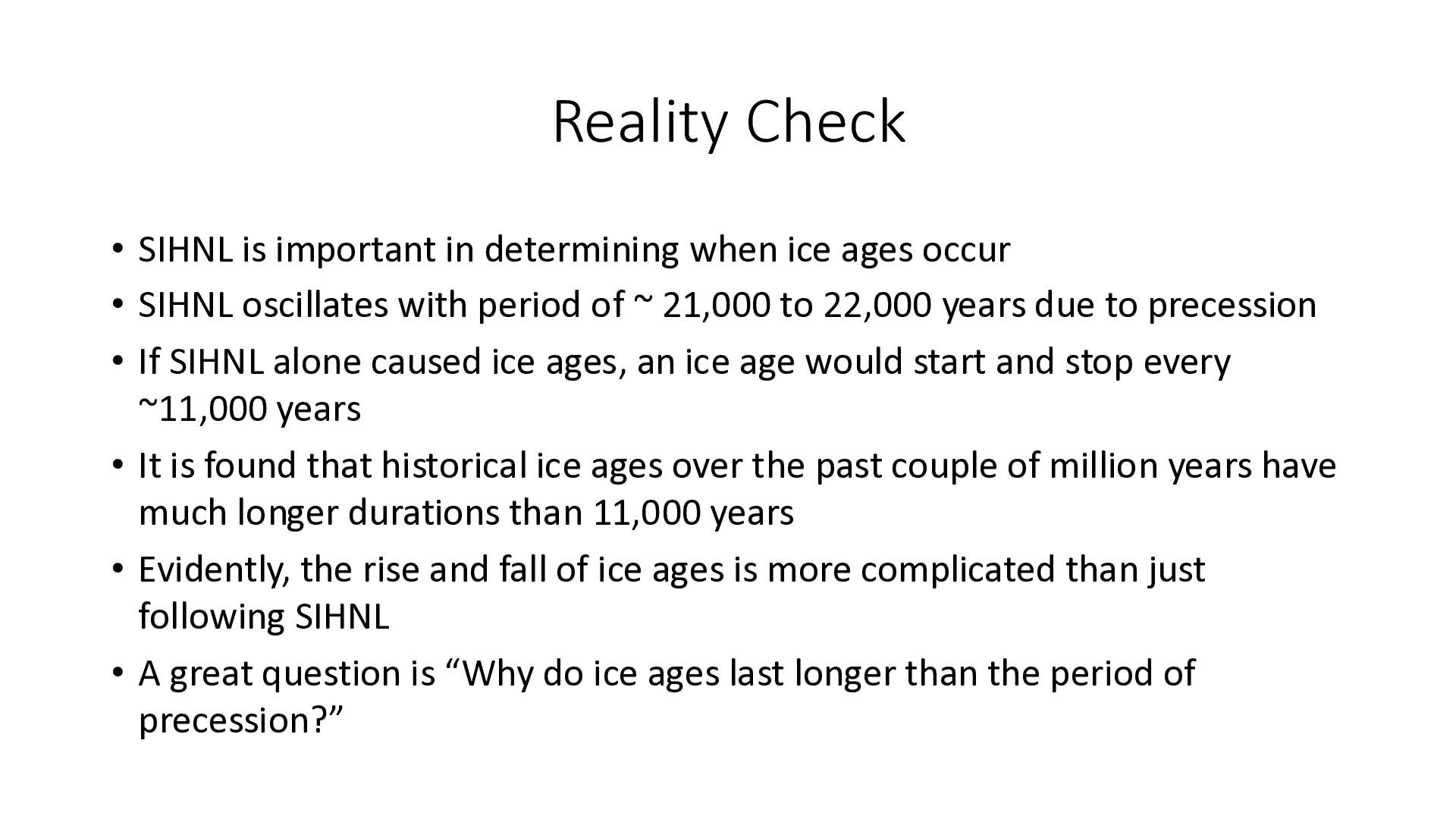
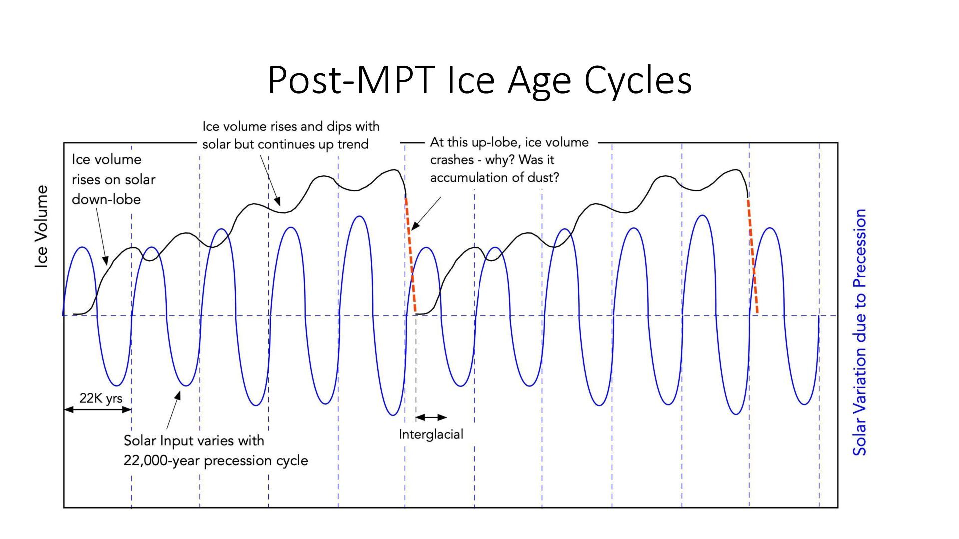
ages occur • SIHNL oscillates with period of ~ 21,000 to 22,000 years due to precession • If SIHNL alone caused ice ages, an ice age would start and stop every ~11,000 years • It is found that historical ice ages over the past couple of million years have much longer durations than 11,000 years • Evidently, the rise and fall of ice ages is more complicated than just following SIHNL • A great question is “Why do ice ages last longer than the period of precession?”
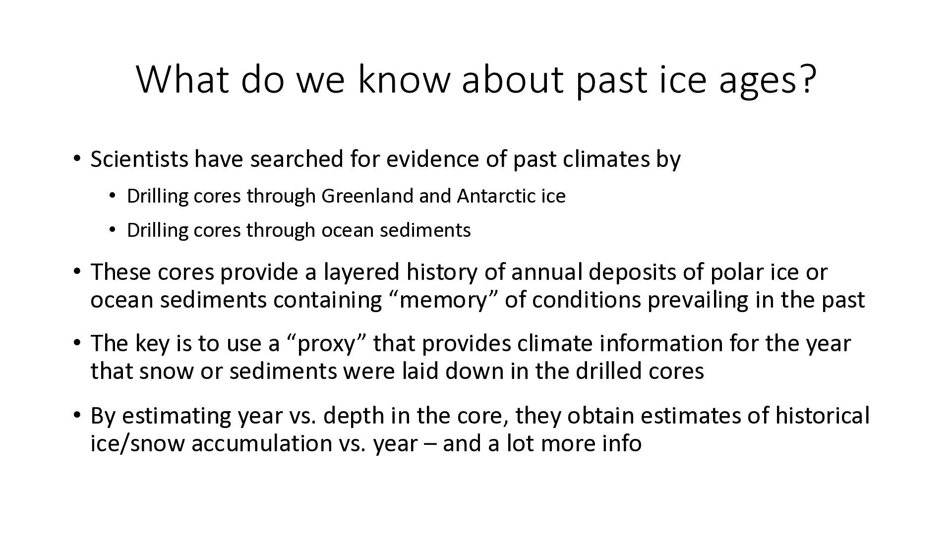
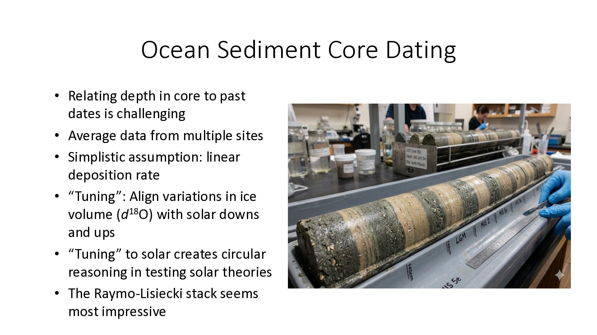
have searched for evidence of past climates by • Drilling cores through Greenland and Antarctic ice • Drilling cores through ocean sediments • These cores provide a layered history of annual deposits of polar ice or ocean sediments containing “memory” of conditions prevailing in the past • The key is to use a “proxy” that provides climate information for the year that snow or sediments were laid down in the drilled cores • By estimating year vs. depth in the core, they obtain estimates of historical ice/snow accumulation vs. year – and a lot more info
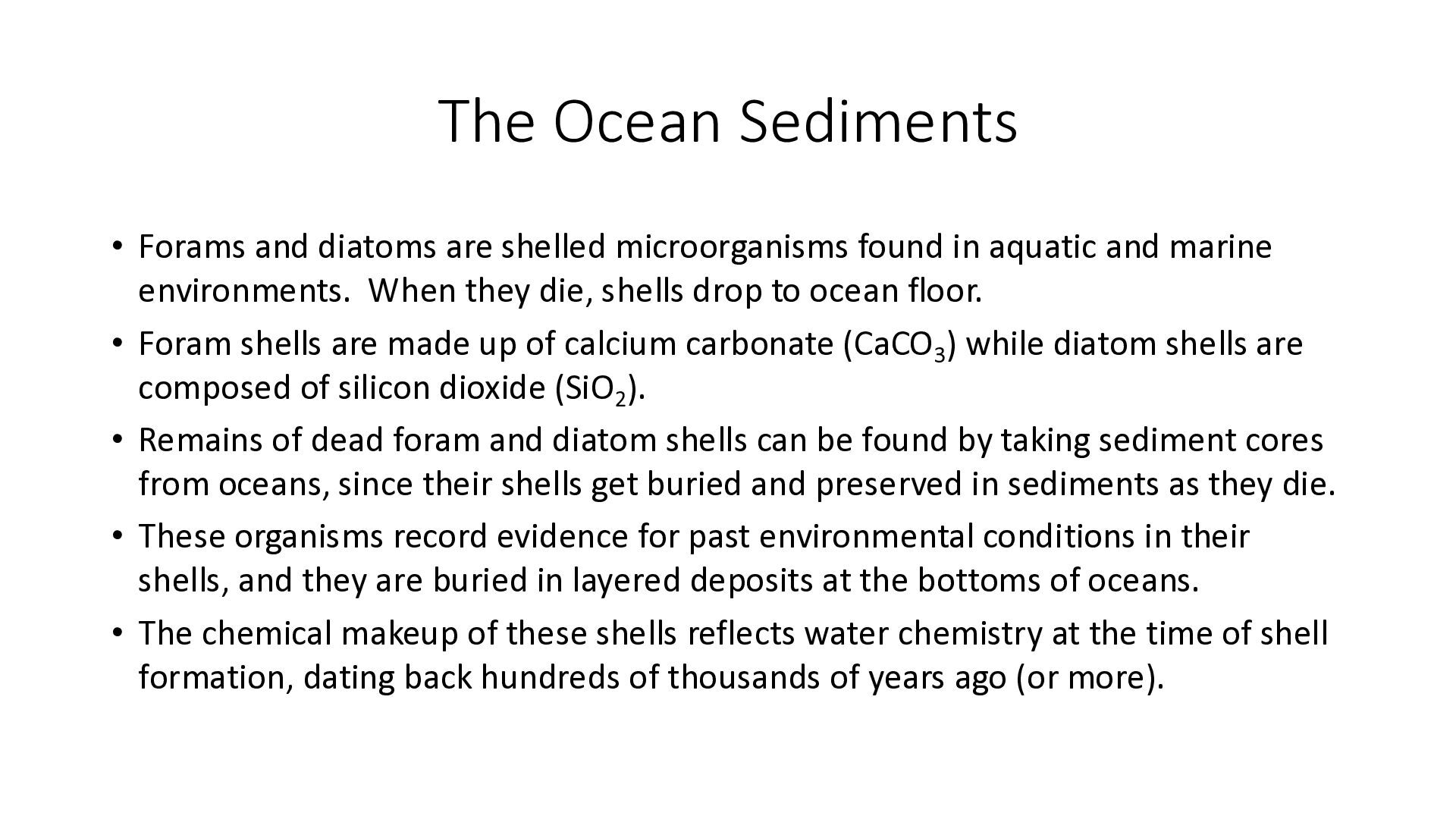
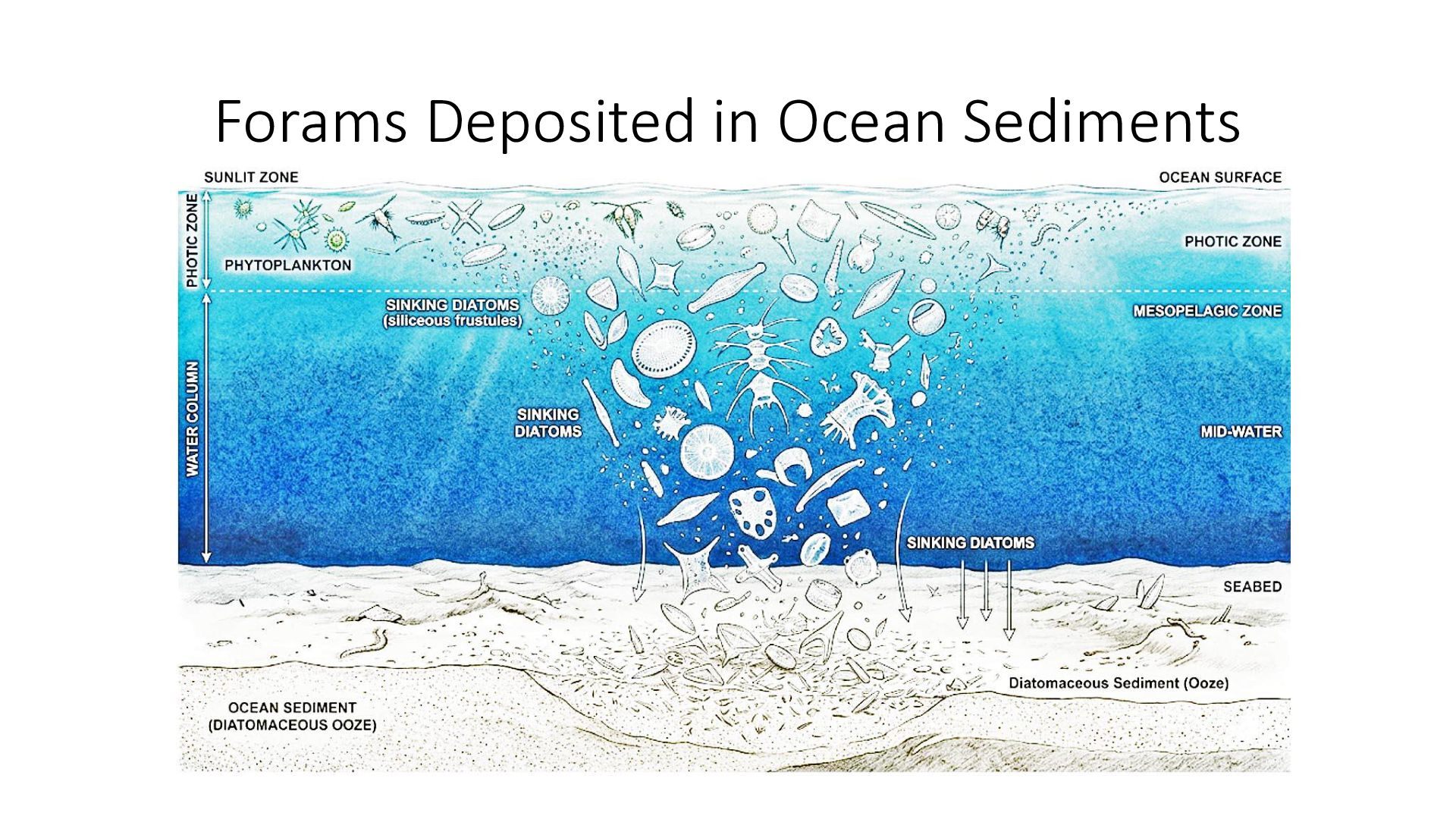
found in aquatic and marine environments. When they die, shells drop to ocean floor. • Foram shells are made up of calcium carbonate (CaCO3) while diatom shells are composed of silicon dioxide (SiO2). • Remains of dead foram and diatom shells can be found by taking sediment cores from oceans, since their shells get buried and preserved in sediments as they die. • These organisms record evidence for past environmental conditions in their shells, and they are buried in layered deposits at the bottoms of oceans. • The chemical makeup of these shells reflects water chemistry at the time of shell formation, dating back hundreds of thousands of years ago (or more).
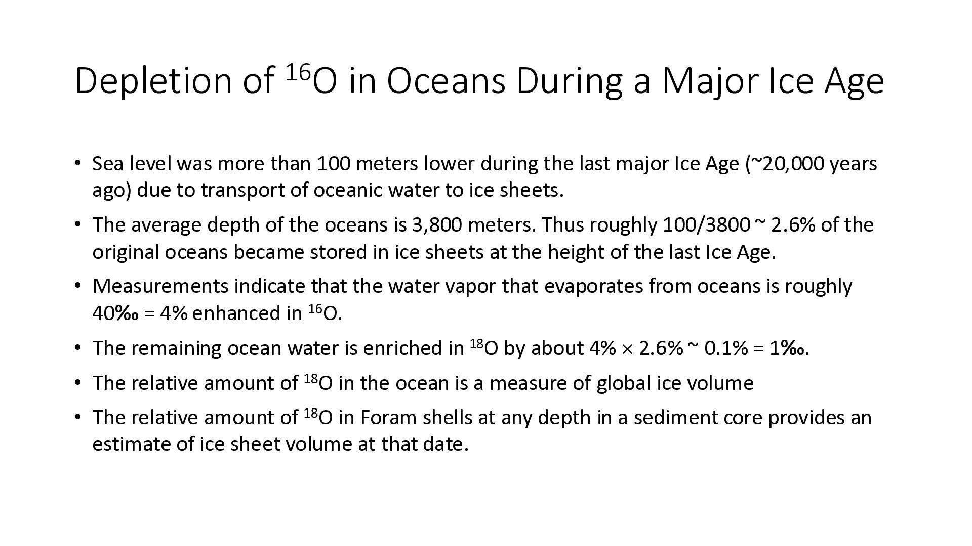
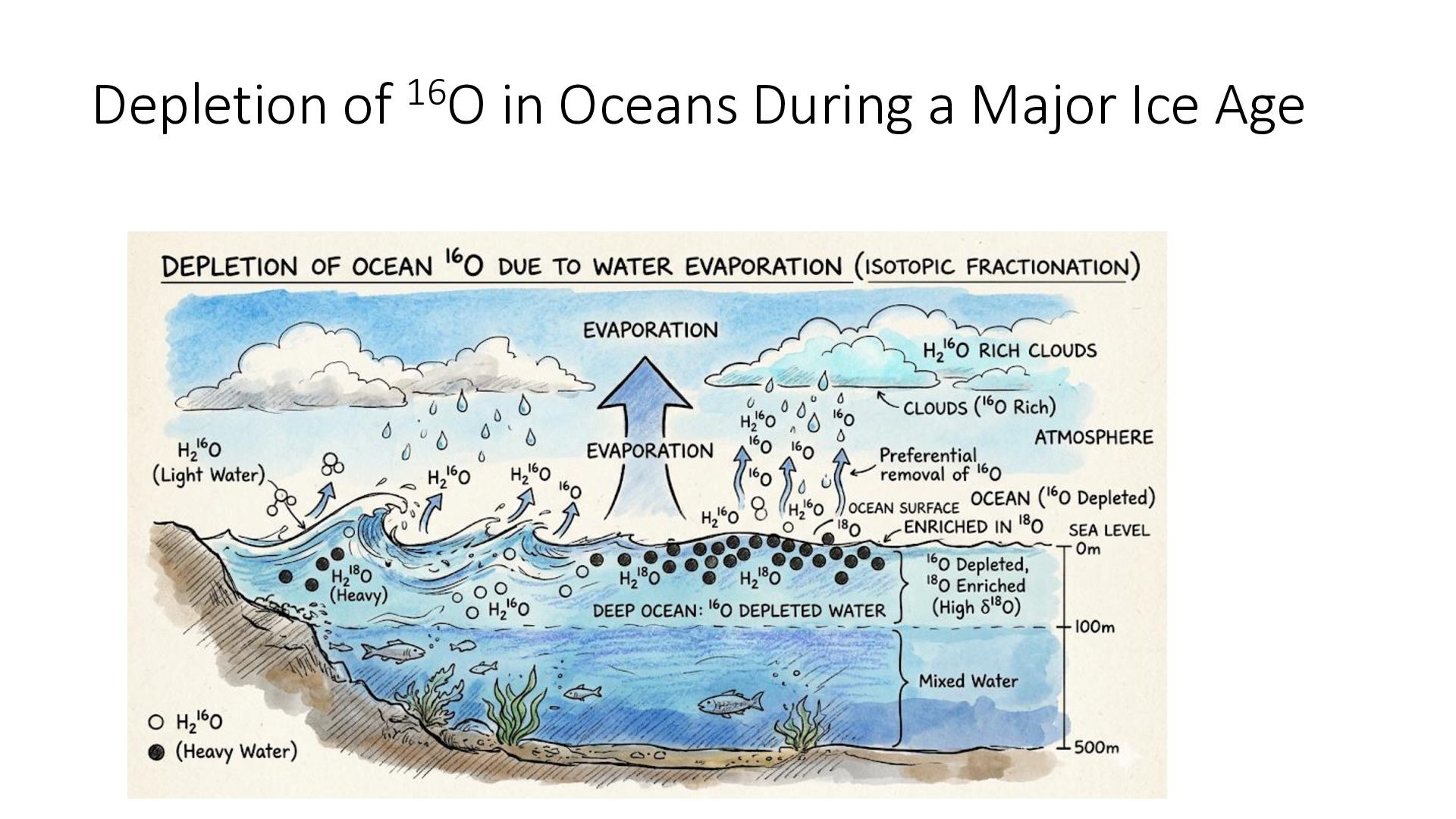
• Sea level was more than 100 meters lower during the last major Ice Age (~20,000 years ago) due to transport of oceanic water to ice sheets. • The average depth of the oceans is 3,800 meters. Thus roughly 100/3800 ~ 2.6% of the original oceans became stored in ice sheets at the height of the last Ice Age. • Measurements indicate that the water vapor that evaporates from oceans is roughly 40‰ = 4% enhanced in 16O. • The remaining ocean water is enriched in 18O by about 4% 2.6% ~ 0.1% = 1‰. • The relative amount of 18O in the ocean is a measure of global ice volume • The relative amount of 18O in Foram shells at any depth in a sediment core provides an estimate of ice sheet volume at that date.
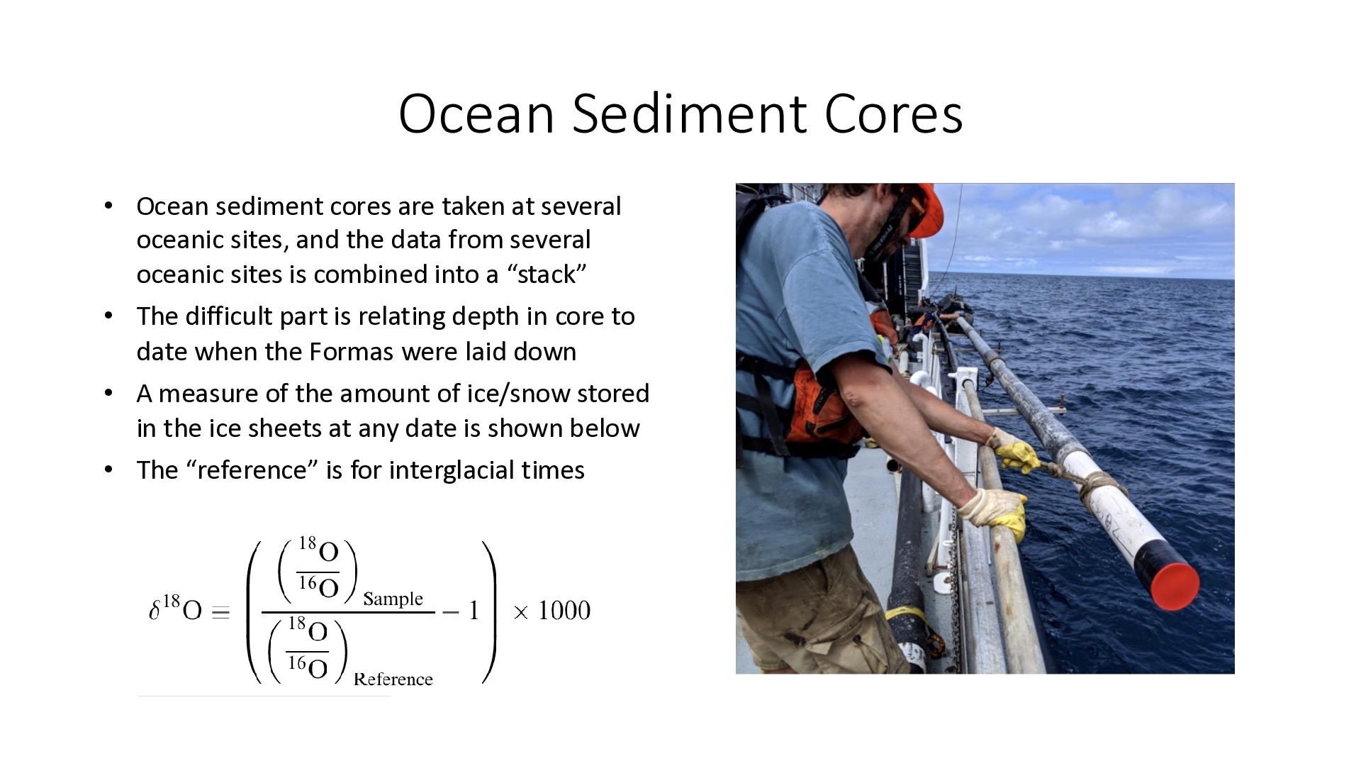
several oceanic sites, and the data from several oceanic sites is combined into a “stack” • The difficult part is relating depth in core to date when the Formas were laid down • A measure of the amount of ice/snow stored in the ice sheets at any date is shown below • The “reference” is for interglacial times
past dates is challenging • Average data from multiple sites • Simplistic assumption: linear deposition rate • “Tuning”: Align variations in ice volume (d18O) with solar downs and ups • “Tuning” to solar creates circular reasoning in testing solar theories • The Raymo-Lisiecki stack seems most impressive
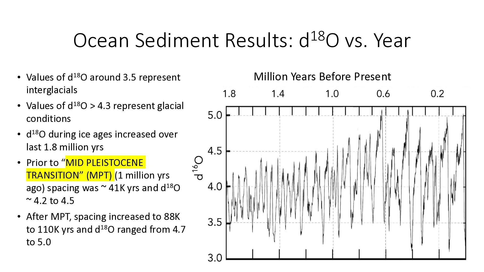
around 3.5 represent interglacials • Values of d18O > 4.3 represent glacial conditions • d18O during ice ages increased over last 1.8 million yrs • Prior to “MID PLEISTOCENE TRANSITION” (MPT) (1 million yrs ago) spacing was ~ 41K yrs and d18O ~ 4.2 to 4.5 • After MPT, spacing increased to 88K to 110K yrs and d18O ranged from 4.7 to 5.0 Million Years Before Present
1.8 million years, the ice/snow at northern sites went through quasi-regular oscillations between interglacial and glacial conditions • Prior to the MPT ( 1 million yrs ago) the cycles were ~ 41K yrs and the ice/snow buildup was limited – but slowly increasing • After the MPT, the cycles were much longer, and the ice/snow buildup was greater than pre-MPT • It is believed from other evidence that during that 1.8-million-year period, the earth was cooling off – aside from periodic ice ages
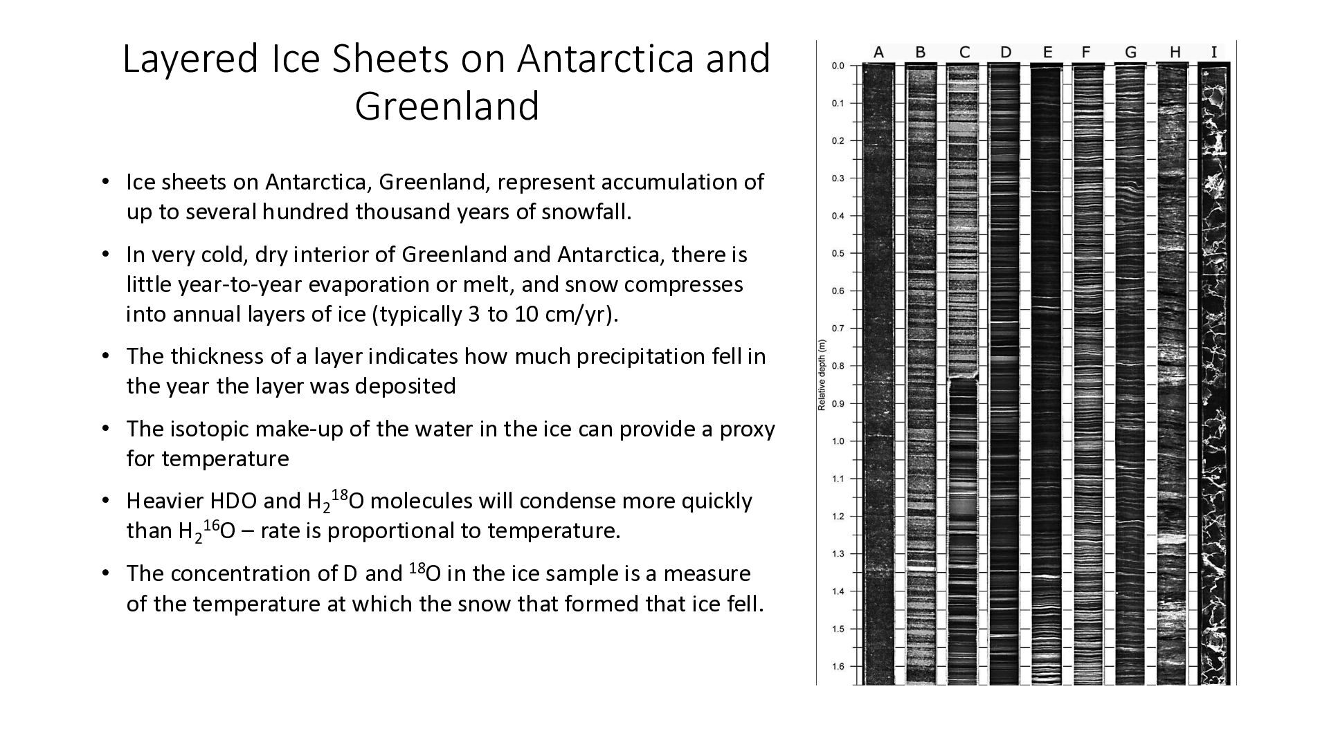
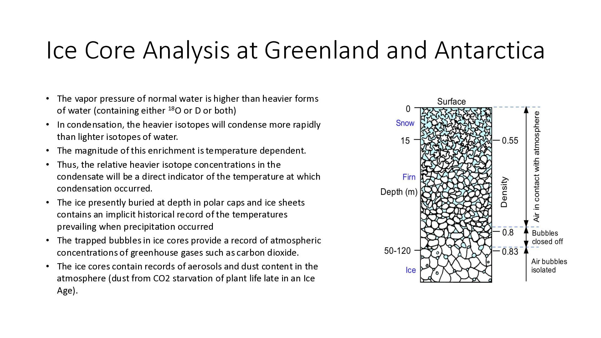
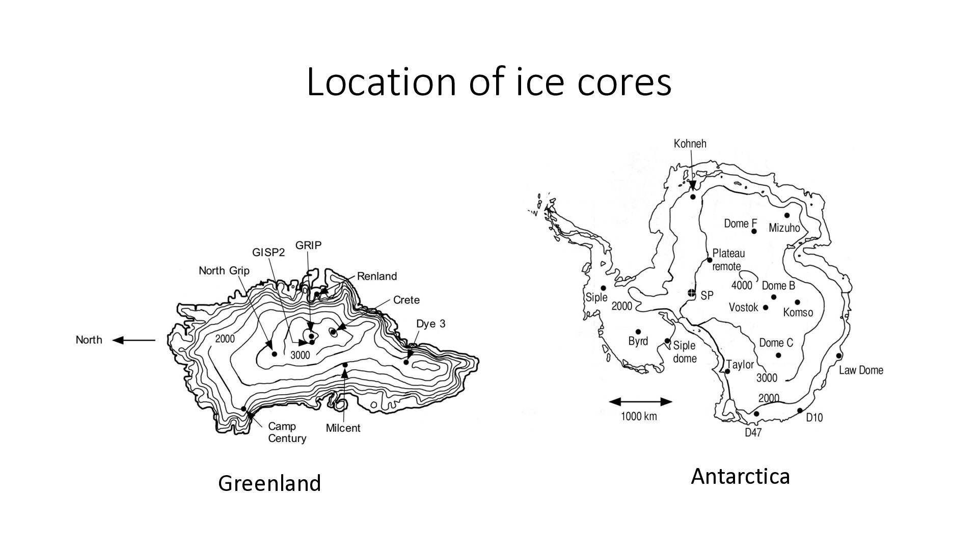
on Antarctica, Greenland, represent accumulation of up to several hundred thousand years of snowfall. • In very cold, dry interior of Greenland and Antarctica, there is little year-to-year evaporation or melt, and snow compresses into annual layers of ice (typically 3 to 10 cm/yr). • The thickness of a layer indicates how much precipitation fell in the year the layer was deposited • The isotopic make-up of the water in the ice can provide a proxy for temperature • Heavier HDO and H218O molecules will condense more quickly than H216O – rate is proportional to temperature. • The concentration of D and 18O in the ice sample is a measure of the temperature at which the snow that formed that ice fell.
pressure of normal water is higher than heavier forms of water (containing either 18O or D or both) • In condensation, the heavier isotopes will condense more rapidly than lighter isotopes of water. • The magnitude of this enrichment is temperature dependent. • Thus, the relative heavier isotope concentrations in the condensate will be a direct indicator of the temperature at which condensation occurred. • The ice presently buried at depth in polar caps and ice sheets contains an implicit historical record of the temperatures prevailing when precipitation occurred • The trapped bubbles in ice cores provide a record of atmospheric concentrations of greenhouse gases such as carbon dioxide. • The ice cores contain records of aerosols and dust content in the atmosphere (dust from CO2 starvation of plant life late in an Ice Age).
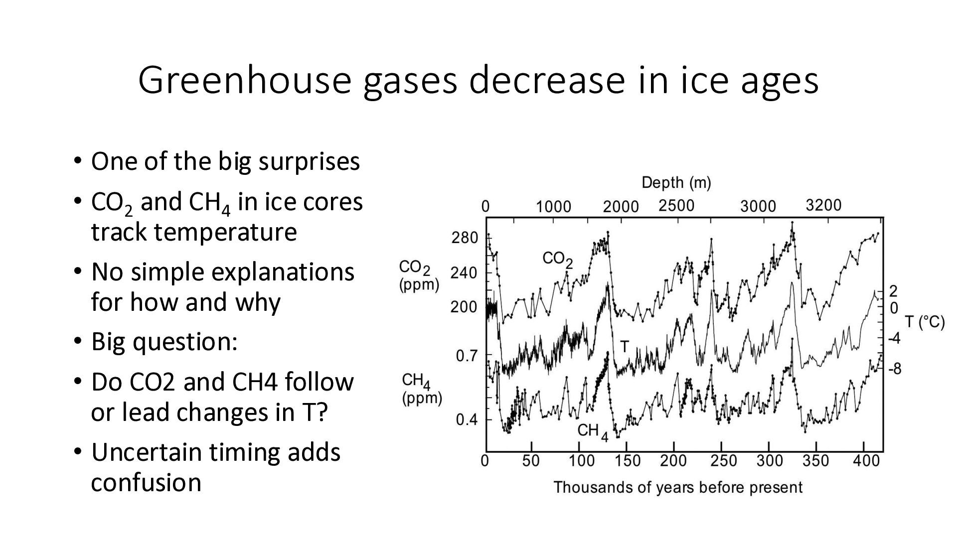
big surprises • CO2 and CH4 in ice cores track temperature • No simple explanations for how and why • Big question: • Do CO2 and CH4 follow or lead changes in T? • Uncertain timing adds confusion
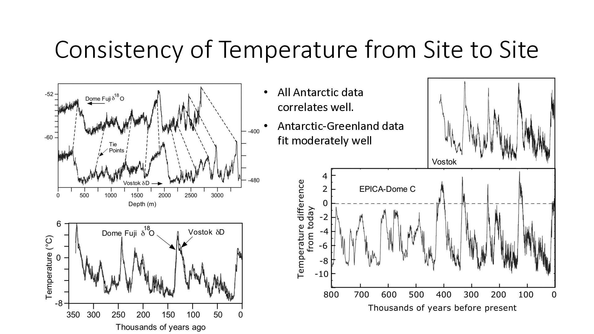
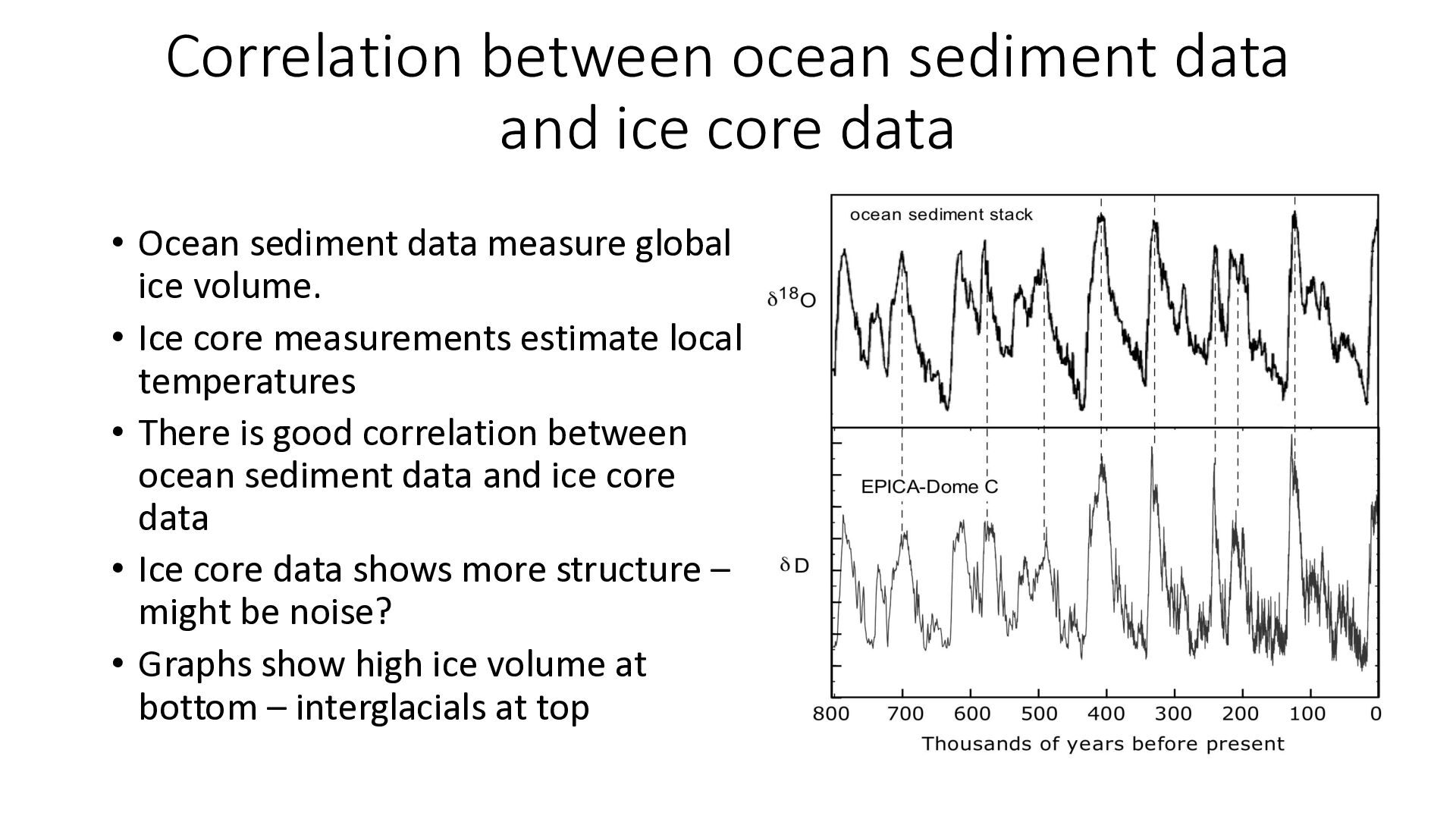
Ocean sediment data measure global ice volume. • Ice core measurements estimate local temperatures • There is good correlation between ocean sediment data and ice core data • Ice core data shows more structure – might be noise? • Graphs show high ice volume at bottom – interglacials at top
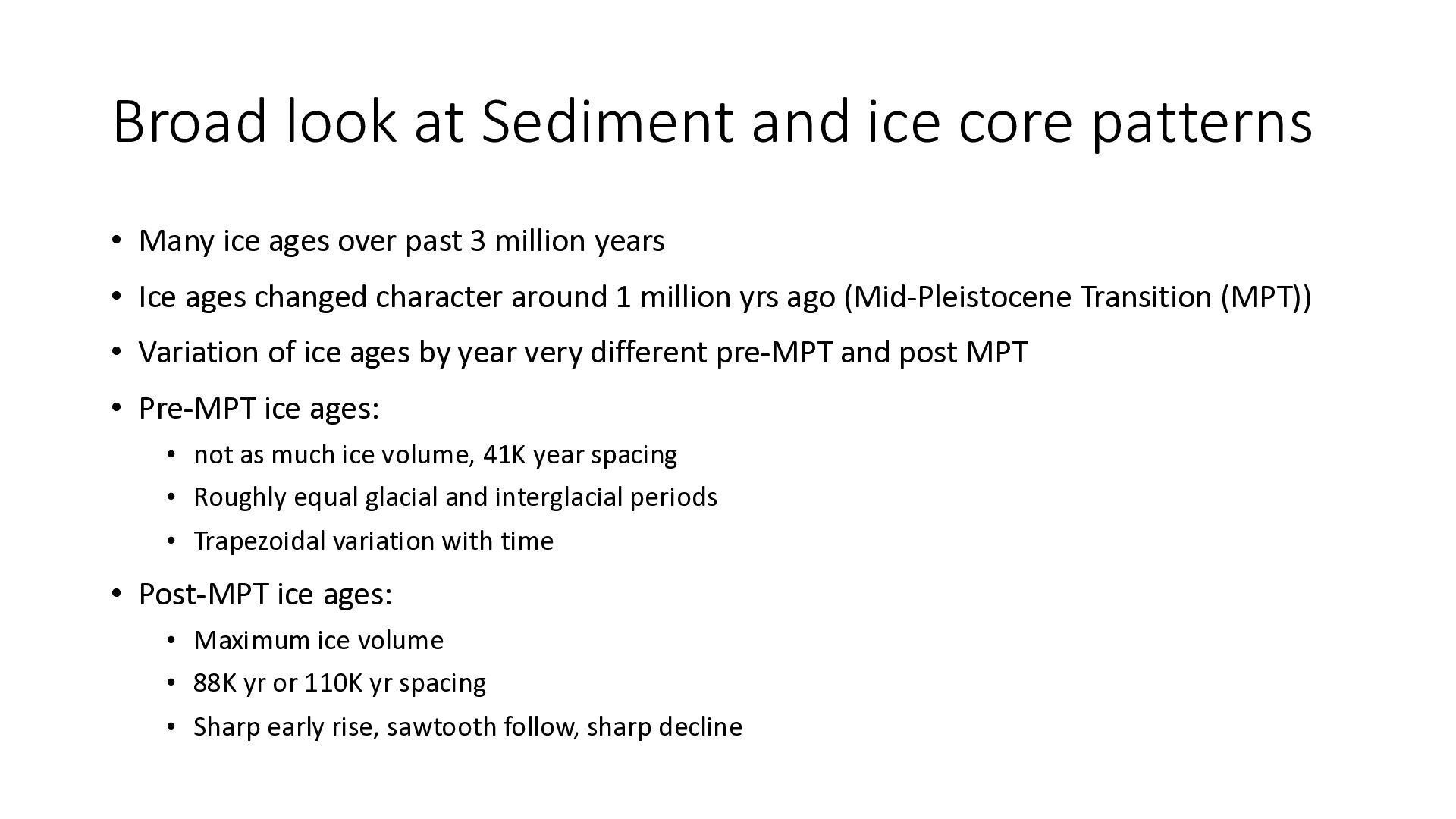
ice ages over past 3 million years • Ice ages changed character around 1 million yrs ago (Mid-Pleistocene Transition (MPT)) • Variation of ice ages by year very different pre-MPT and post MPT • Pre-MPT ice ages: • not as much ice volume, 41K year spacing • Roughly equal glacial and interglacial periods • Trapezoidal variation with time • Post-MPT ice ages: • Maximum ice volume • 88K yr or 110K yr spacing • Sharp early rise, sawtooth follow, sharp decline
utilizing many different inputs • Difficult to comprehend except by a few specialists • To the great extent that dating depends on alignment with variations in SIHNL, called “tuning”, this makes it problematic for testing the solar theories – circular reasoning • The ocean sediment stack derived by Raymo and Lisiecki is probably the best dataset
cases, experts do not seem to have observed the data patterns properly • In the pre-MPT, nobody seems to have noticed the form of time dependence being trapezoidal with roughly equal glacial and interglacial periods – they did emphasize 41K year period • In the post-MPT, they did not notice that the spacing was a multiple of 22K yrs (88K or 110K) and most simply claimed it was about 100K. (Maureen Raymo was a single exception.) • In the post-MPT, they did not take note of the very rapid initial increase in ice volume, but only seemed to see the later, slower “sawtooth” increase.
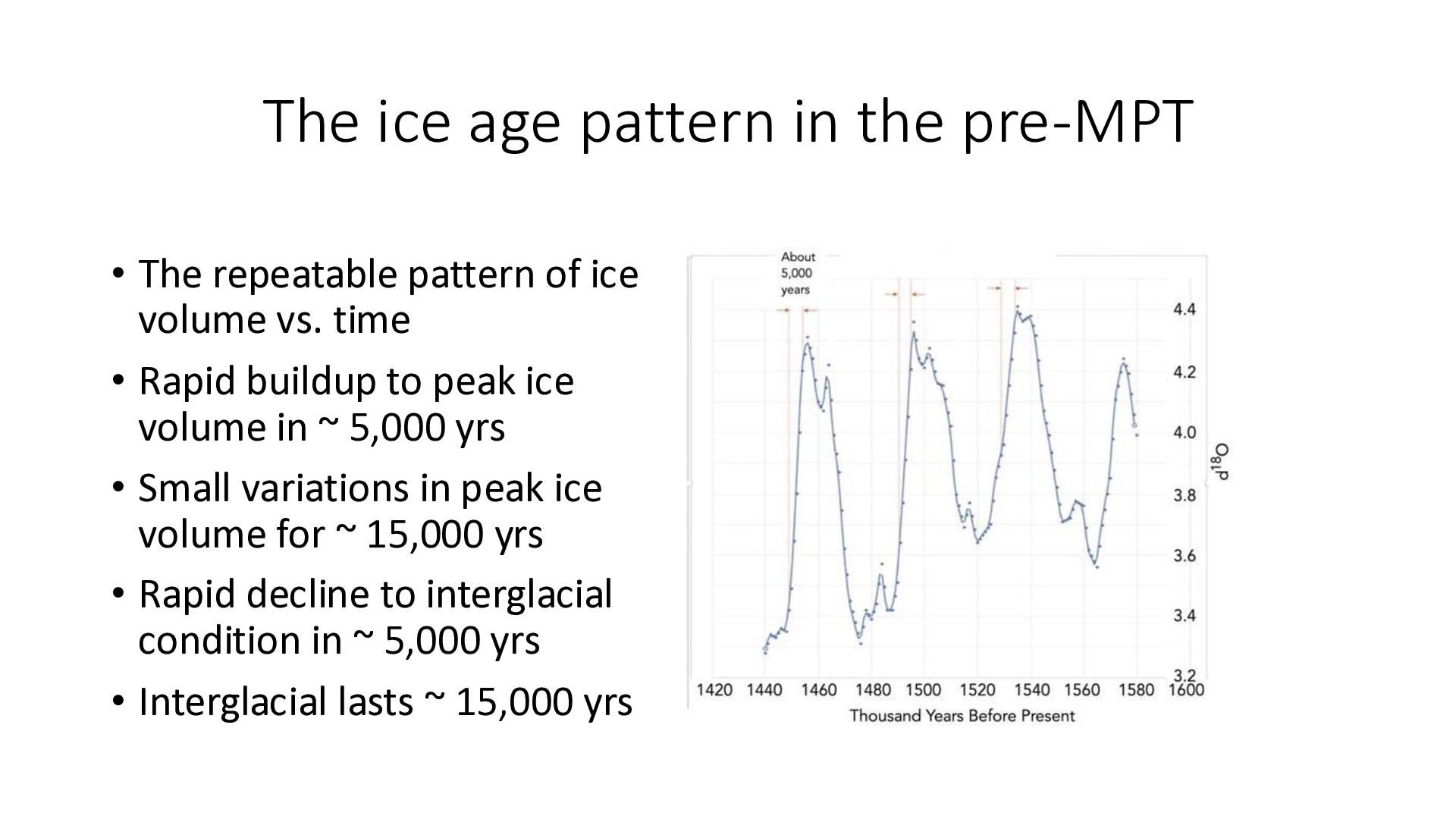
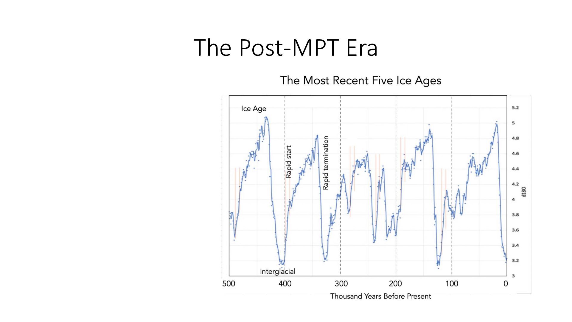
pattern of ice volume vs. time • Rapid buildup to peak ice volume in ~ 5,000 yrs • Small variations in peak ice volume for ~ 15,000 yrs • Rapid decline to interglacial condition in ~ 5,000 yrs • Interglacial lasts ~ 15,000 yrs
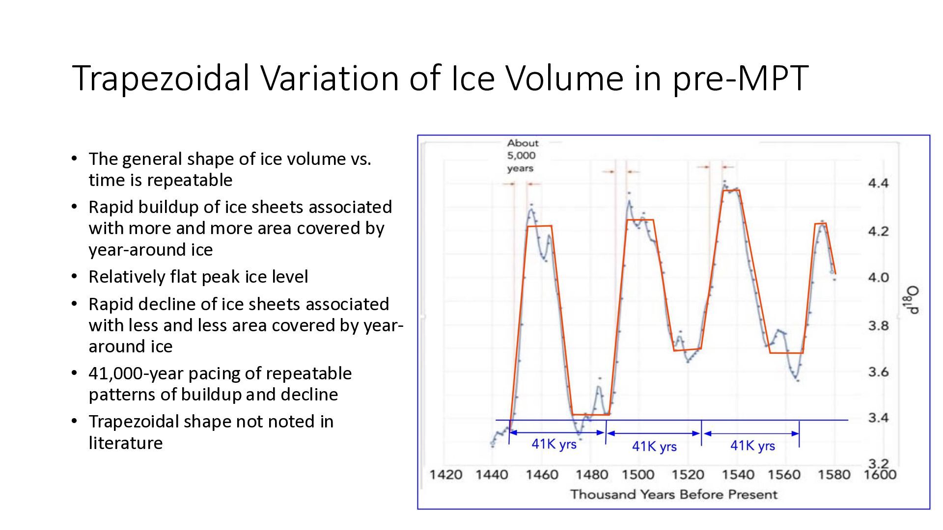
shape of ice volume vs. time is repeatable • Rapid buildup of ice sheets associated with more and more area covered by year-around ice • Relatively flat peak ice level • Rapid decline of ice sheets associated with less and less area covered by yeararound ice • 41,000-year pacing of repeatable patterns of buildup and decline • Trapezoidal shape not noted in literature
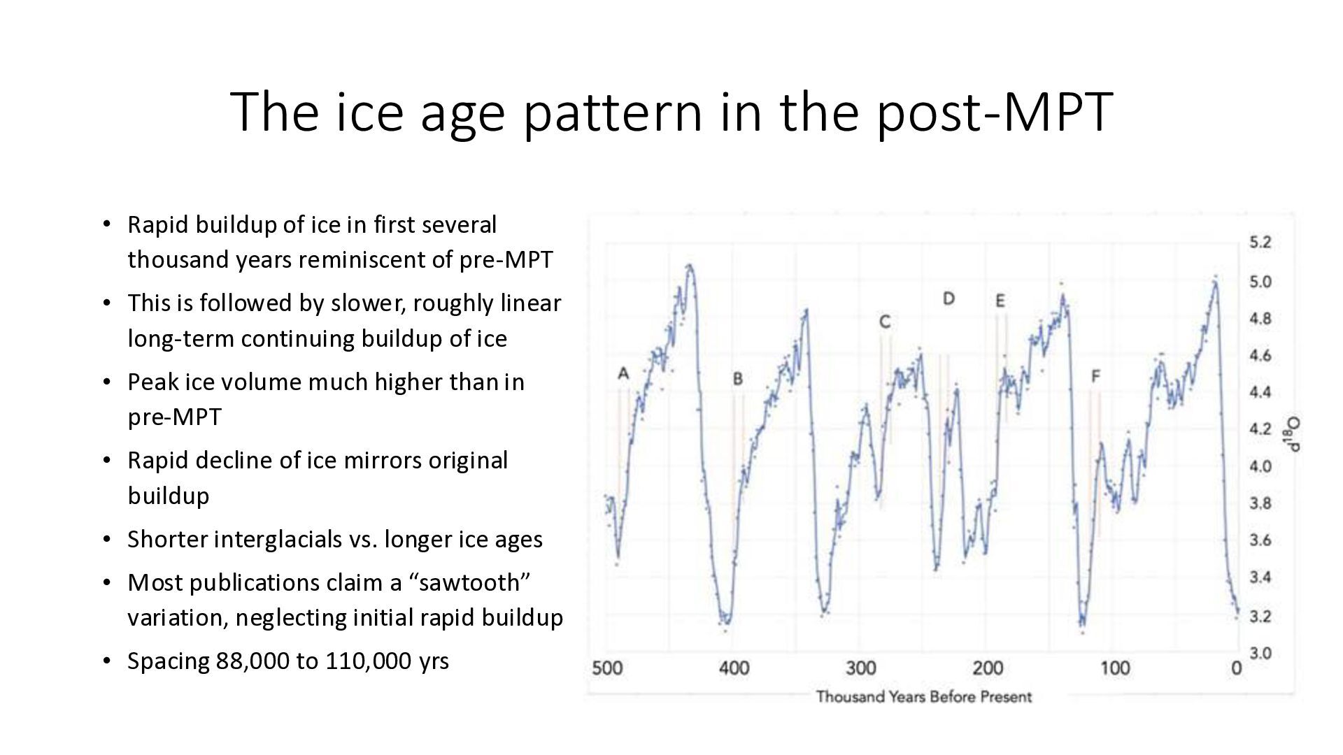
of ice in first several thousand years reminiscent of pre-MPT • This is followed by slower, roughly linear long-term continuing buildup of ice • Peak ice volume much higher than in pre-MPT • Rapid decline of ice mirrors original buildup • Shorter interglacials vs. longer ice ages • Most publications claim a “sawtooth” variation, neglecting initial rapid buildup • Spacing 88,000 to 110,000 yrs
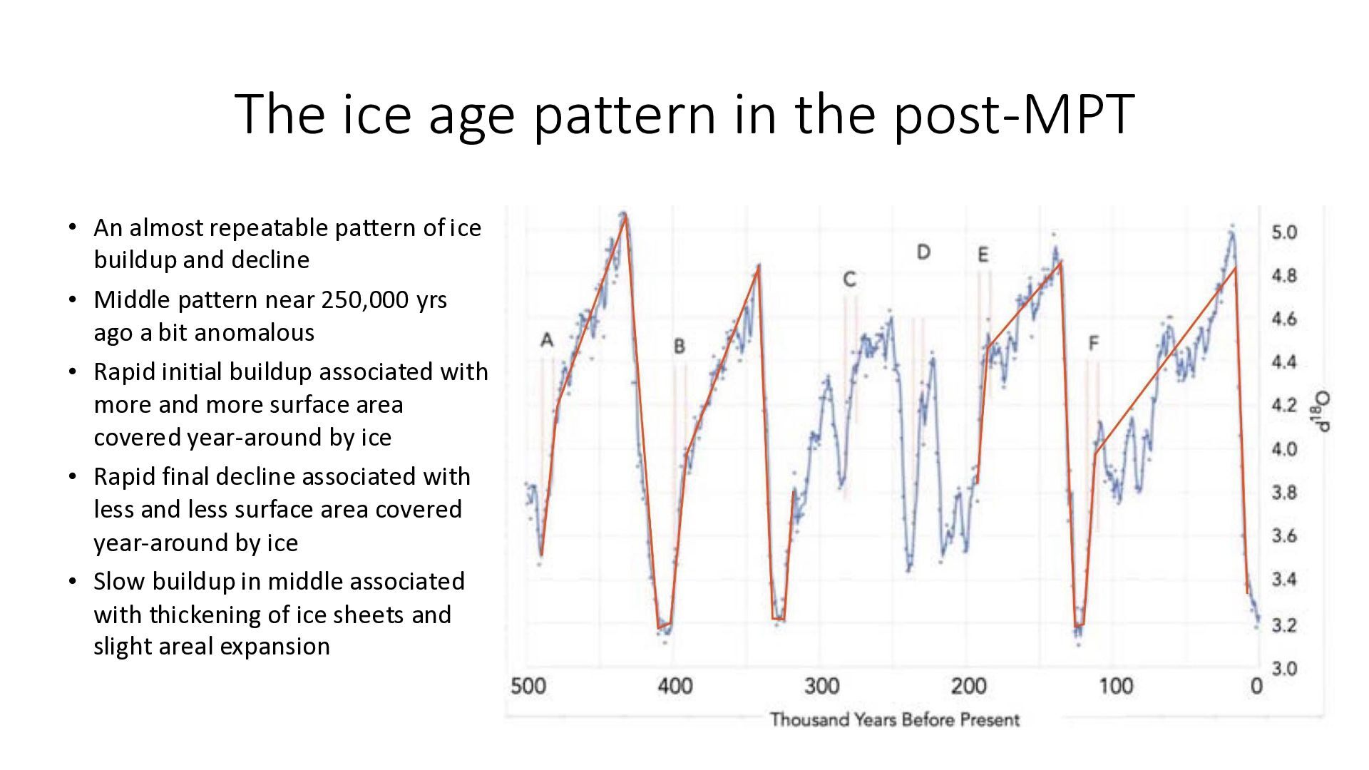
repeatable pattern of ice buildup and decline • Middle pattern near 250,000 yrs ago a bit anomalous • Rapid initial buildup associated with more and more surface area covered year-around by ice • Rapid final decline associated with less and less surface area covered year-around by ice • Slow buildup in middle associated with thickening of ice sheets and slight areal expansion
Ice age analysts can’t see straight? It pays to look at the data? • The accepted common narrative is expressed by AI (and it is wrong): • “Climate records of ice ages show a distinct ‘sawtooth’ pattern, where global temperatures decrease gradually over tens of thousands of years, followed by an abrupt, rapid warming that ends the ice age. This asymmetry shows slow ice sheet growth and rapid melting.” • The actual pattern consists of three phases: • Phase 1: Very rapid initial rate of accumulation of ice in ice sheets • Phase 2: Long-term gradual slowing of rate of accumulation of ice in ice sheets • Phase 3: Mirror image of Phase 1 with rapid decline of ice extent
both pre-MPT and post-MPT, initial buildup and decline of ice ages is similar with rapid change to and from glacial conditions in 4,000 to 8,000 years • Initial buildup and termination are like mirror images of one another • Such rapid buildup and decline is associated with increased or decreased surface area that is covered with snow/ice year-around • Maximum ice volume in post-MPT is significantly greater than in pre-MPT era • Repeatable patterns occur in both eras, but they are different • The period of repeatability in the pre-MPT is ~ 41,000 yrs and in the post-MPT it is about 88,000 to 110,000 yrs • The form of the ice volume vs time in the pre-MPT is trapezoidal, while in the post-MPT it is rapid buildup, followed by long slow accumulation
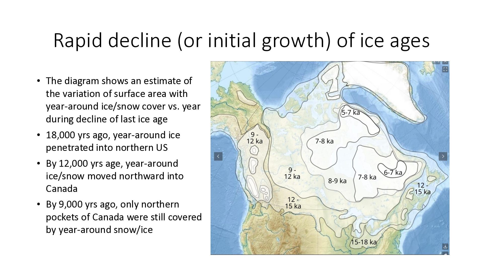
diagram shows an estimate of the variation of surface area with year-around ice/snow cover vs. year during decline of last ice age • 18,000 yrs ago, year-around ice penetrated into northern US • By 12,000 yrs age, year-around ice/snow moved northward into Canada • By 9,000 yrs ago, only northern pockets of Canada were still covered by year-around snow/ice
they do • The SIHNL is believed to be a factor in ice age cycles • The SIHNL oscillates with precession at ~ 22,000 years • Yet ice age cycles have much longer periods • The cycles change from before to after the MPT • It is known that the earth in general cooled over the last few thousand years • Any model or explanation for cycles must treat pre-MPT and post-MPT separately • Some models estimate dV/dt (rate of change of ice volume) and integrate this over time. They don’t work well.
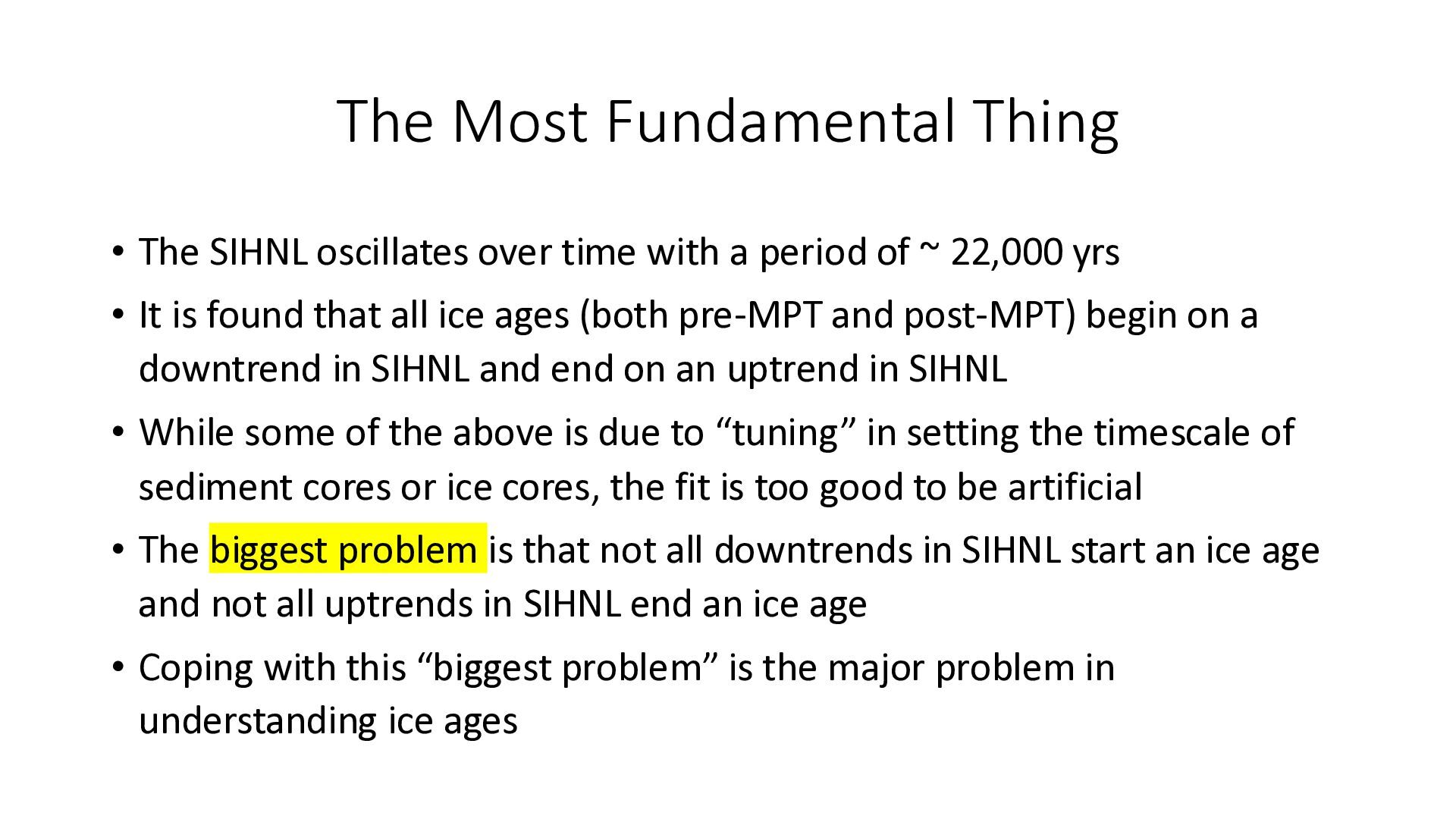
with a period of ~ 22,000 yrs • It is found that all ice ages (both pre-MPT and post-MPT) begin on a downtrend in SIHNL and end on an uptrend in SIHNL • While some of the above is due to “tuning” in setting the timescale of sediment cores or ice cores, the fit is too good to be artificial • The biggest problem is that not all downtrends in SIHNL start an ice age and not all uptrends in SIHNL end an ice age • Coping with this “biggest problem” is the major problem in understanding ice ages
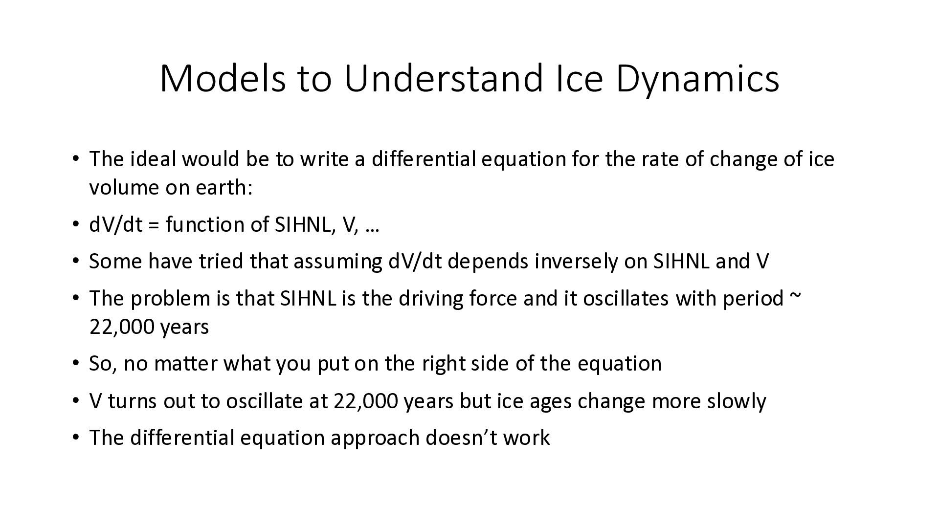
to write a differential equation for the rate of change of ice volume on earth: • dV/dt = function of SIHNL, V, … • Some have tried that assuming dV/dt depends inversely on SIHNL and V • The problem is that SIHNL is the driving force and it oscillates with period ~ 22,000 years • So, no matter what you put on the right side of the equation • V turns out to oscillate at 22,000 years but ice ages change more slowly • The differential equation approach doesn’t work
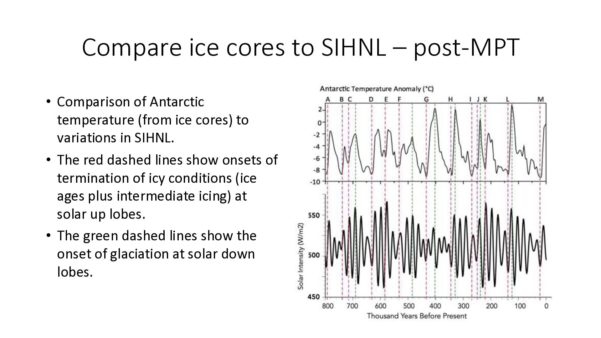
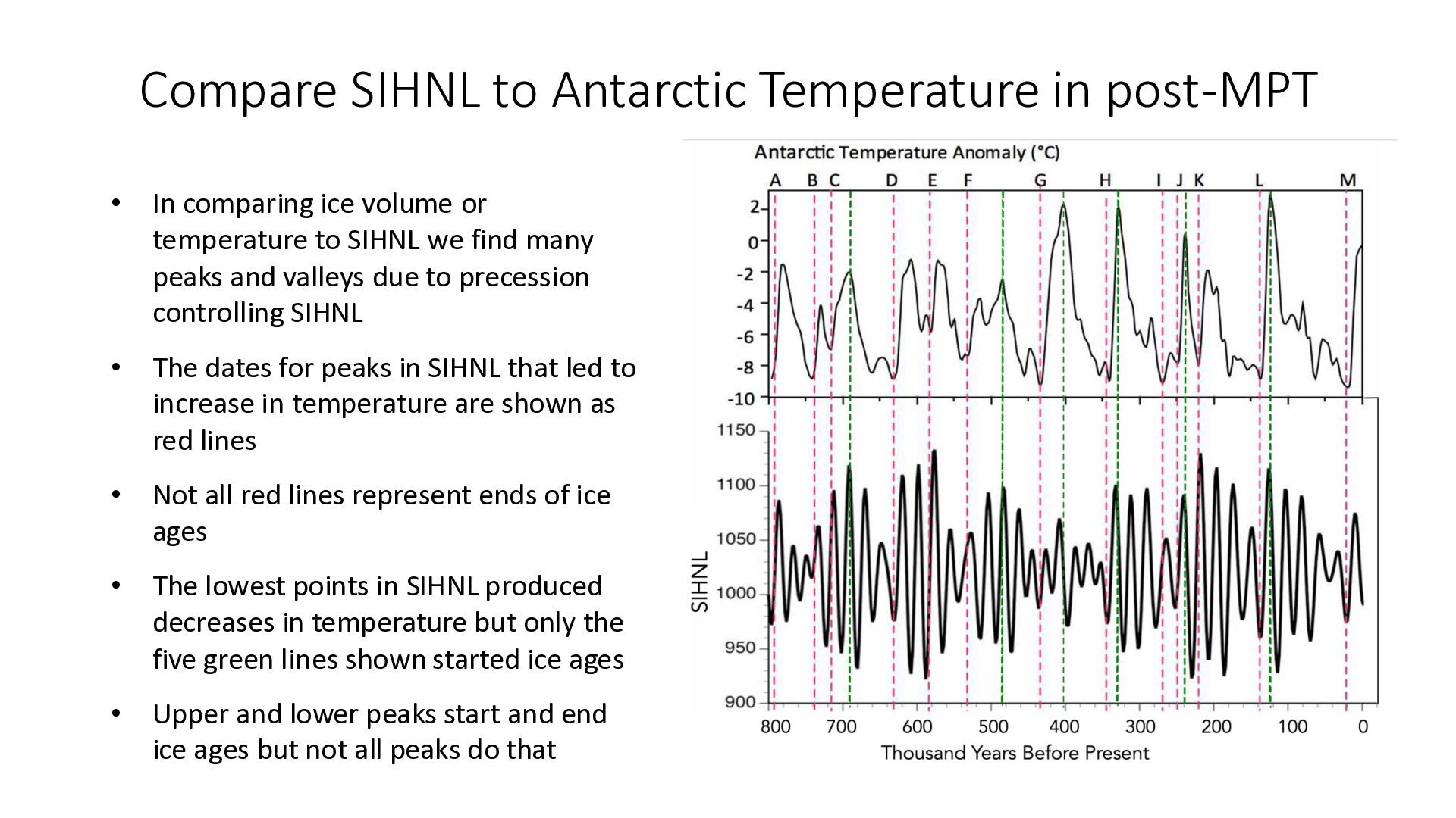
Antarctic temperature (from ice cores) to variations in SIHNL. • The red dashed lines show onsets of termination of icy conditions (ice ages plus intermediate icing) at solar up lobes. • The green dashed lines show the onset of glaciation at solar down lobes.
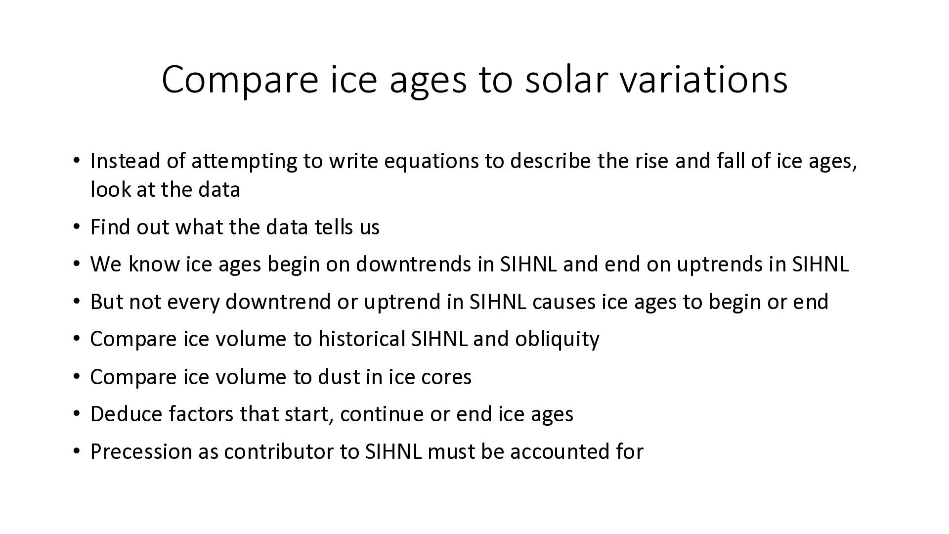
to write equations to describe the rise and fall of ice ages, look at the data • Find out what the data tells us • We know ice ages begin on downtrends in SIHNL and end on uptrends in SIHNL • But not every downtrend or uptrend in SIHNL causes ice ages to begin or end • Compare ice volume to historical SIHNL and obliquity • Compare ice volume to dust in ice cores • Deduce factors that start, continue or end ice ages • Precession as contributor to SIHNL must be accounted for
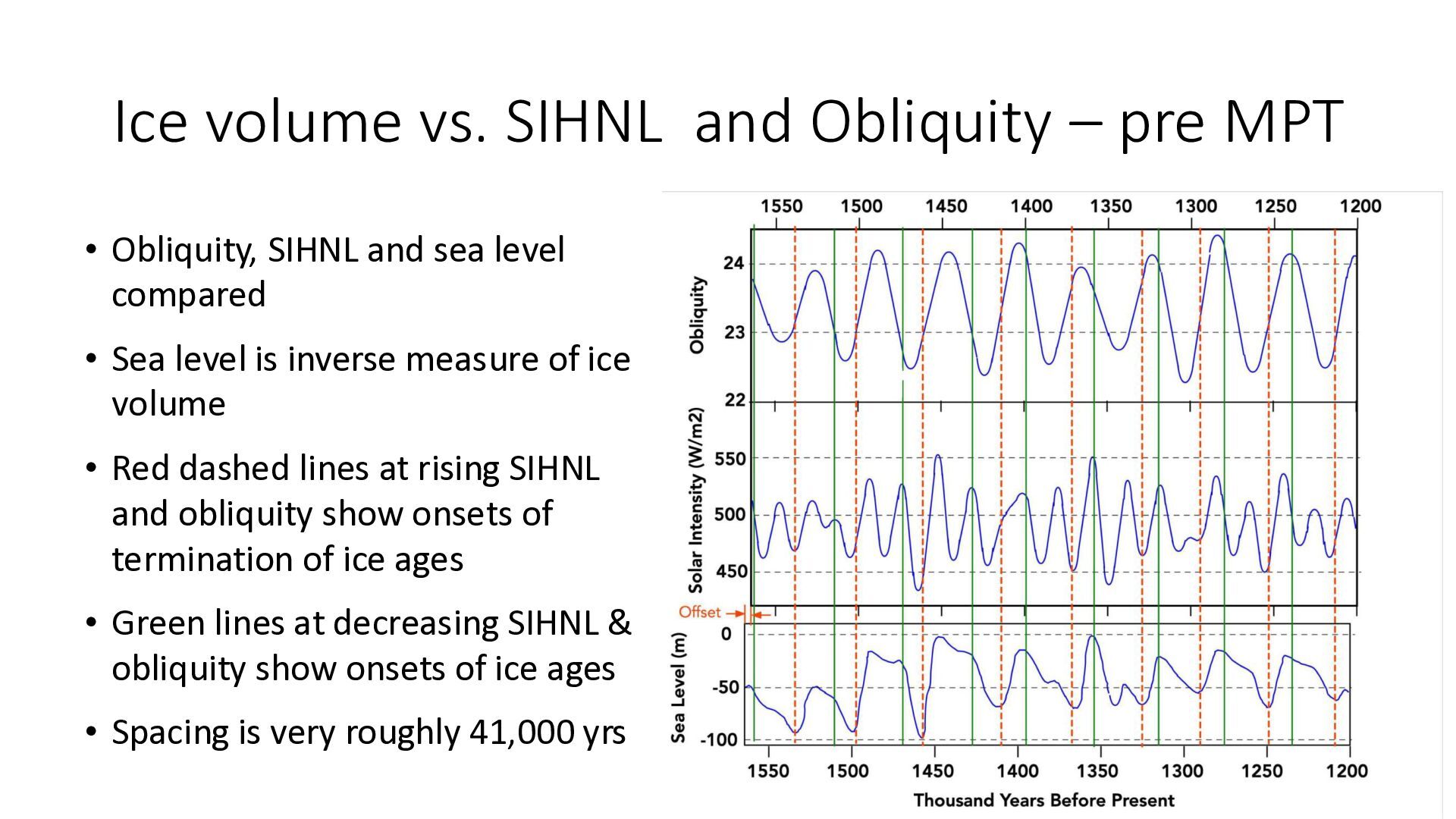
Obliquity, SIHNL and sea level compared • Sea level is inverse measure of ice volume • Red dashed lines at rising SIHNL and obliquity show onsets of termination of ice ages • Green lines at decreasing SIHNL & obliquity show onsets of ice ages • Spacing is very roughly 41,000 yrs
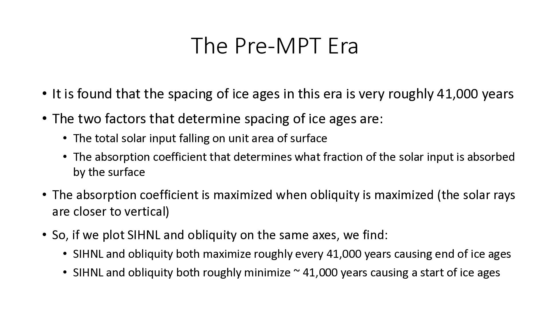
of ice ages in this era is very roughly 41,000 years • The two factors that determine spacing of ice ages are: • The total solar input falling on unit area of surface • The absorption coefficient that determines what fraction of the solar input is absorbed by the surface • The absorption coefficient is maximized when obliquity is maximized (the solar rays are closer to vertical) • So, if we plot SIHNL and obliquity on the same axes, we find: • SIHNL and obliquity both maximize roughly every 41,000 years causing end of ice ages • SIHNL and obliquity both roughly minimize ~ 41,000 years causing a start of ice ages
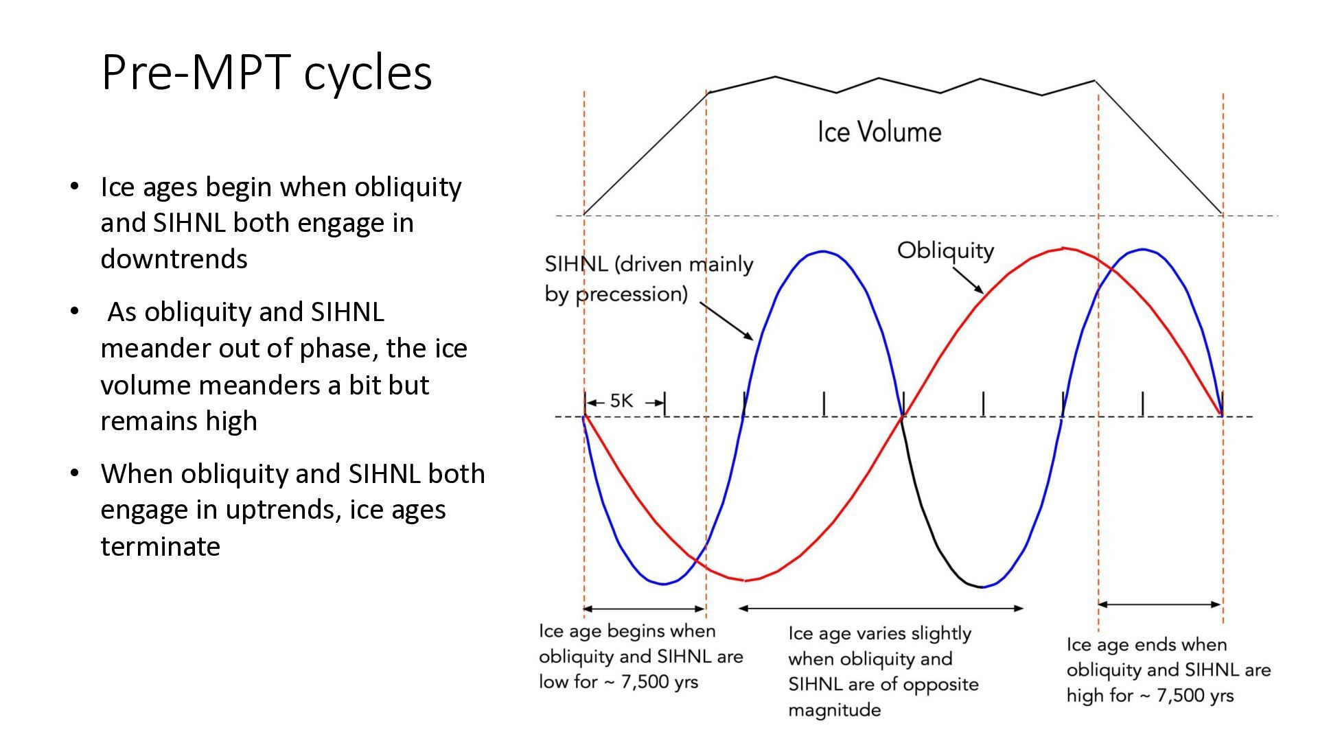
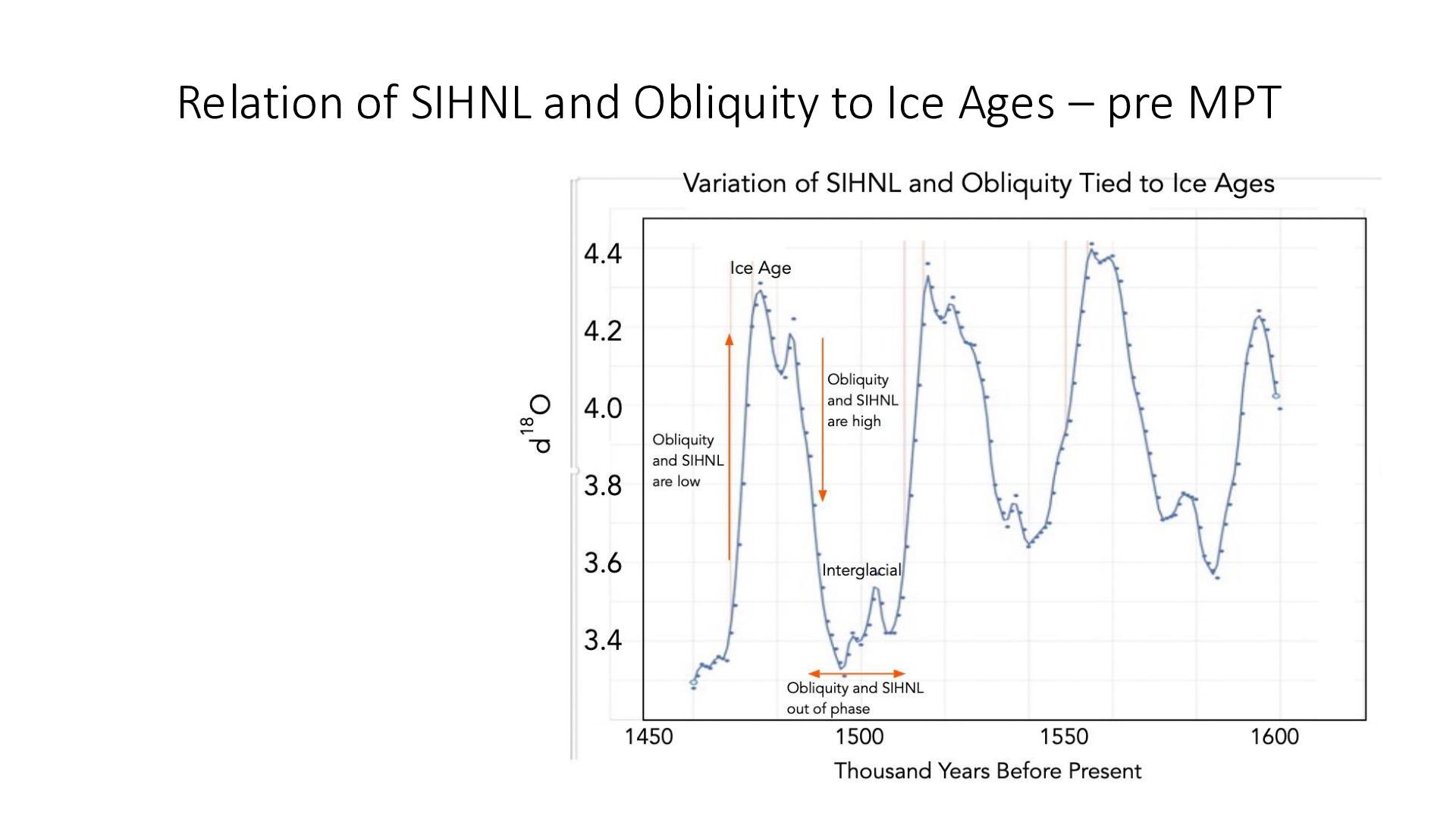
both engage in downtrends • As obliquity and SIHNL meander out of phase, the ice volume meanders a bit but remains high • When obliquity and SIHNL both engage in uptrends, ice ages terminate
cooled over the past two million years • Over the past two million years, the earth was in an ice age more than 50% of the time • The cooling was enhanced by repeated occurrence of ice ages that increased reflectivity and drew down CO2 and GHG • In the pre-MPT, ice volume was constrained by occurrence of high SIHNL and obliquity in the same time era causing termination after about 41,000 years • In the post-MPT, it was cold enough that enough that ice built up rapidly in the early years to survive occurrence of high SIHNL and obliquity in the same time era, and ice continued to build up beyond 41,000 years
ice volume or temperature to SIHNL we find many peaks and valleys due to precession controlling SIHNL • The dates for peaks in SIHNL that led to increase in temperature are shown as red lines • Not all red lines represent ends of ice ages • The lowest points in SIHNL produced decreases in temperature but only the five green lines shown started ice ages • Upper and lower peaks start and end ice ages but not all peaks do that
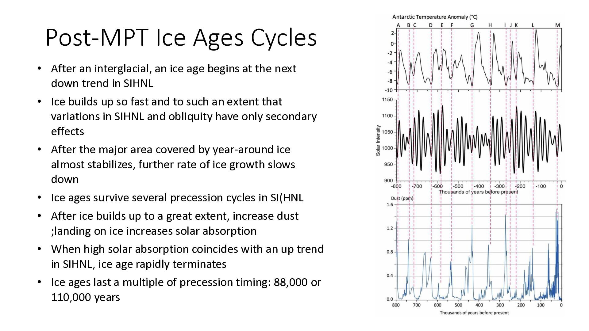
age begins at the next down trend in SIHNL • Ice builds up so fast and to such an extent that variations in SIHNL and obliquity have only secondary effects • After the major area covered by year-around ice almost stabilizes, further rate of ice growth slows down • Ice ages survive several precession cycles in SI(HNL • After ice builds up to a great extent, increase dust ;landing on ice increases solar absorption • When high solar absorption coincides with an up trend in SIHNL, ice age rapidly terminates • Ice ages last a multiple of precession timing: 88,000 or 110,000 years
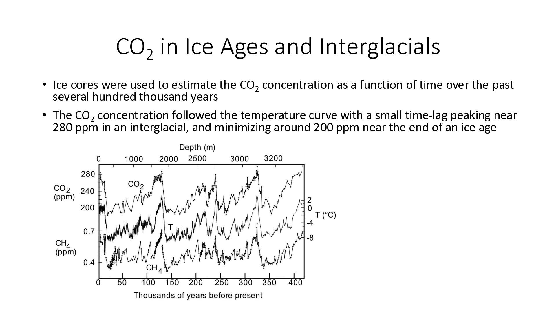
used to estimate the CO2 concentration as a function of time over the past several hundred thousand years • The CO2 concentration followed the temperature curve with a small time-lag peaking near 280 ppm in an interglacial, and minimizing around 200 ppm near the end of an ice age
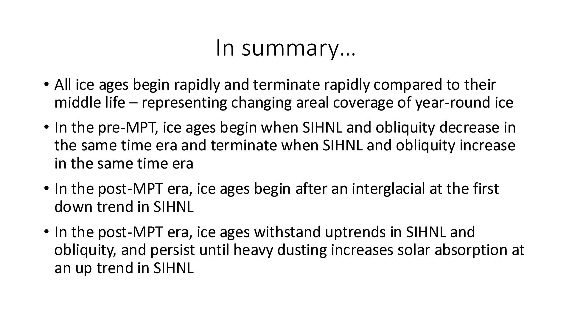
rapidly compared to their middle life – representing changing areal coverage of year-round ice • In the pre-MPT, ice ages begin when SIHNL and obliquity decrease in the same time era and terminate when SIHNL and obliquity increase in the same time era • In the post-MPT era, ice ages begin after an interglacial at the first down trend in SIHNL • In the post-MPT era, ice ages withstand uptrends in SIHNL and obliquity, and persist until heavy dusting increases solar absorption at an up trend in SIHNL
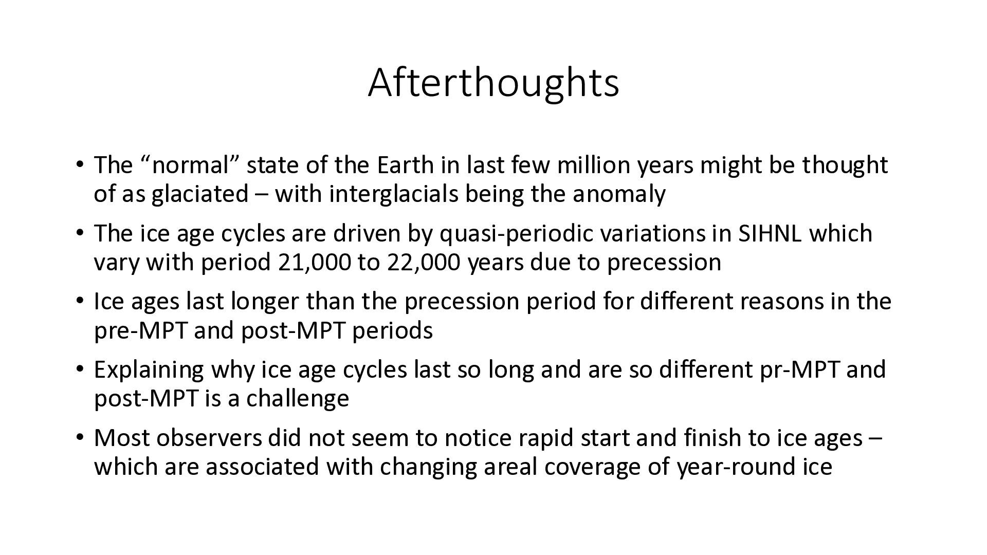
few million years might be thought of as glaciated – with interglacials being the anomaly • The ice age cycles are driven by quasi-periodic variations in SIHNL which vary with period 21,000 to 22,000 years due to precession • Ice ages last longer than the precession period for different reasons in the pre-MPT and post-MPT periods • Explaining why ice age cycles last so long and are so different pr-MPT and post-MPT is a challenge • Most observers did not seem to notice rapid start and finish to ice ages – which are associated with changing areal coverage of year-round ice


 rmaruy
 takusamar
 akasan
 michielstock
 tagtag
 tsoh
 xleitix
 institutdelelevage
 trycycle
 sshimizu2006
 bonotake
 coloredviolet
 reverentgeek
 addyosmani
 inesmontani
 chrislema
 codingconduct
 nmsamuel
 portentint
 lauravandoore
 marcduiker
 twada
 tammyeverts