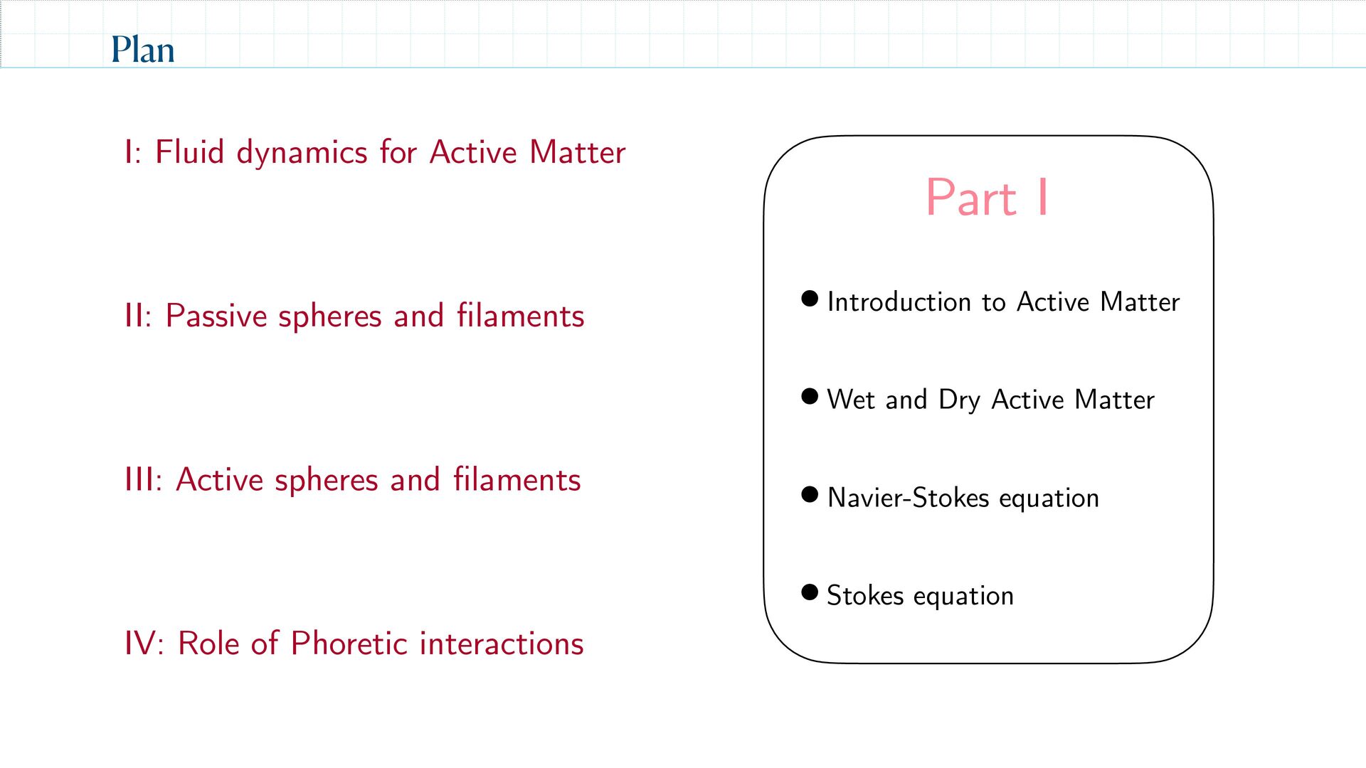
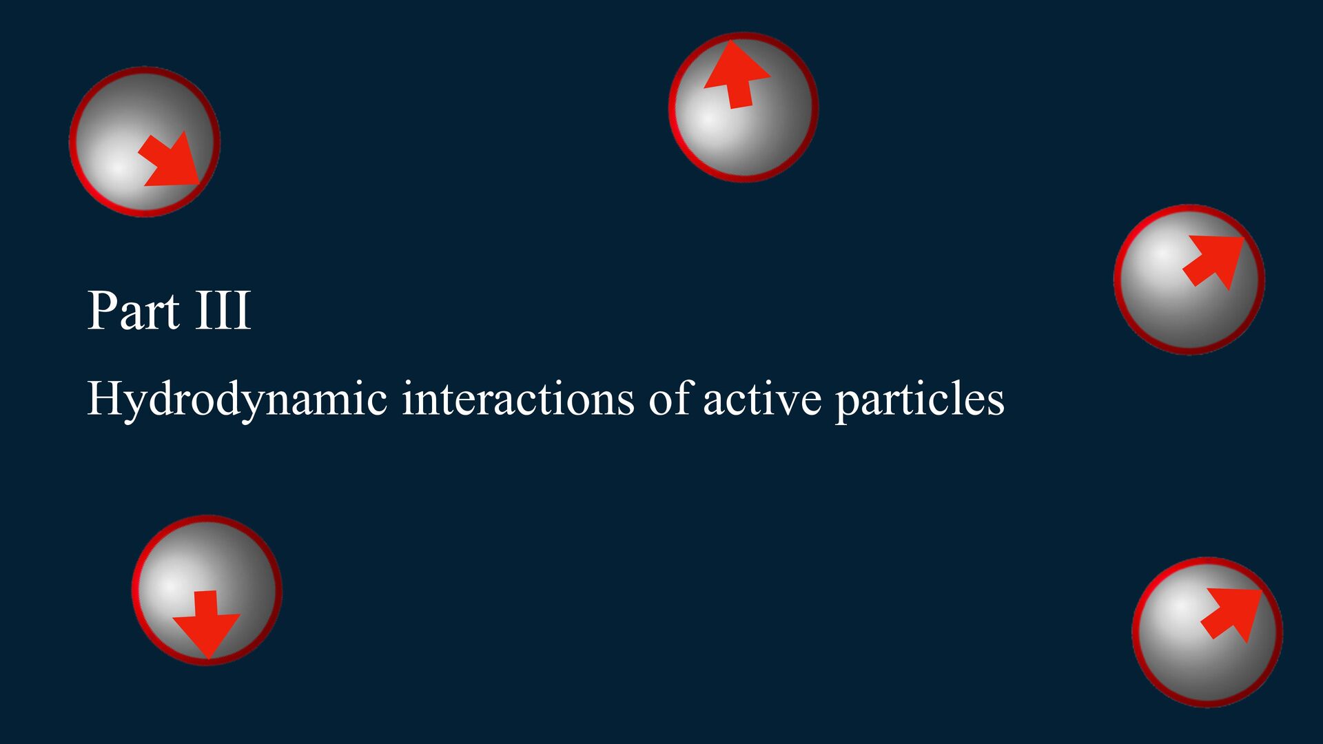
Dry Active Matter • Navier-Stokes equation • Stokes equation Part I I: Fluid dynamics for Active Matter II: Passive spheres and filaments IV: Role of Phoretic interactions III: Active spheres and filaments
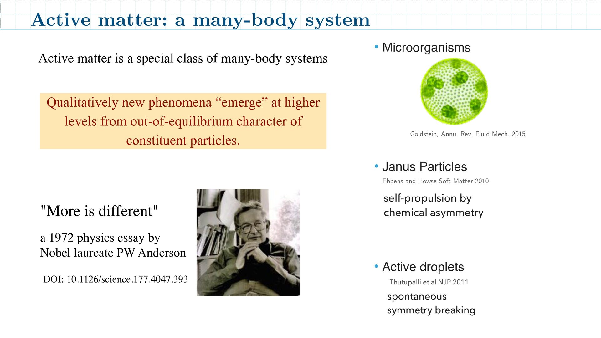
class of many-body systems DOI: 10.1126/science.177.4047.393 "More is different" a 1972 physics essay by Nobel laureate PW Anderson Qualitatively new phenomena “emerge” at higher levels from out-of-equilibrium character of constituent particles. • Microorganisms Goldstein, Annu. Rev. Fluid Mech. 2015 spontaneous symmetry breaking • Active droplets Thutupalli et al NJP 2011 self-propulsion by chemical asymmetry • Janus Particles Ebbens and Howse Soft Matter 2010
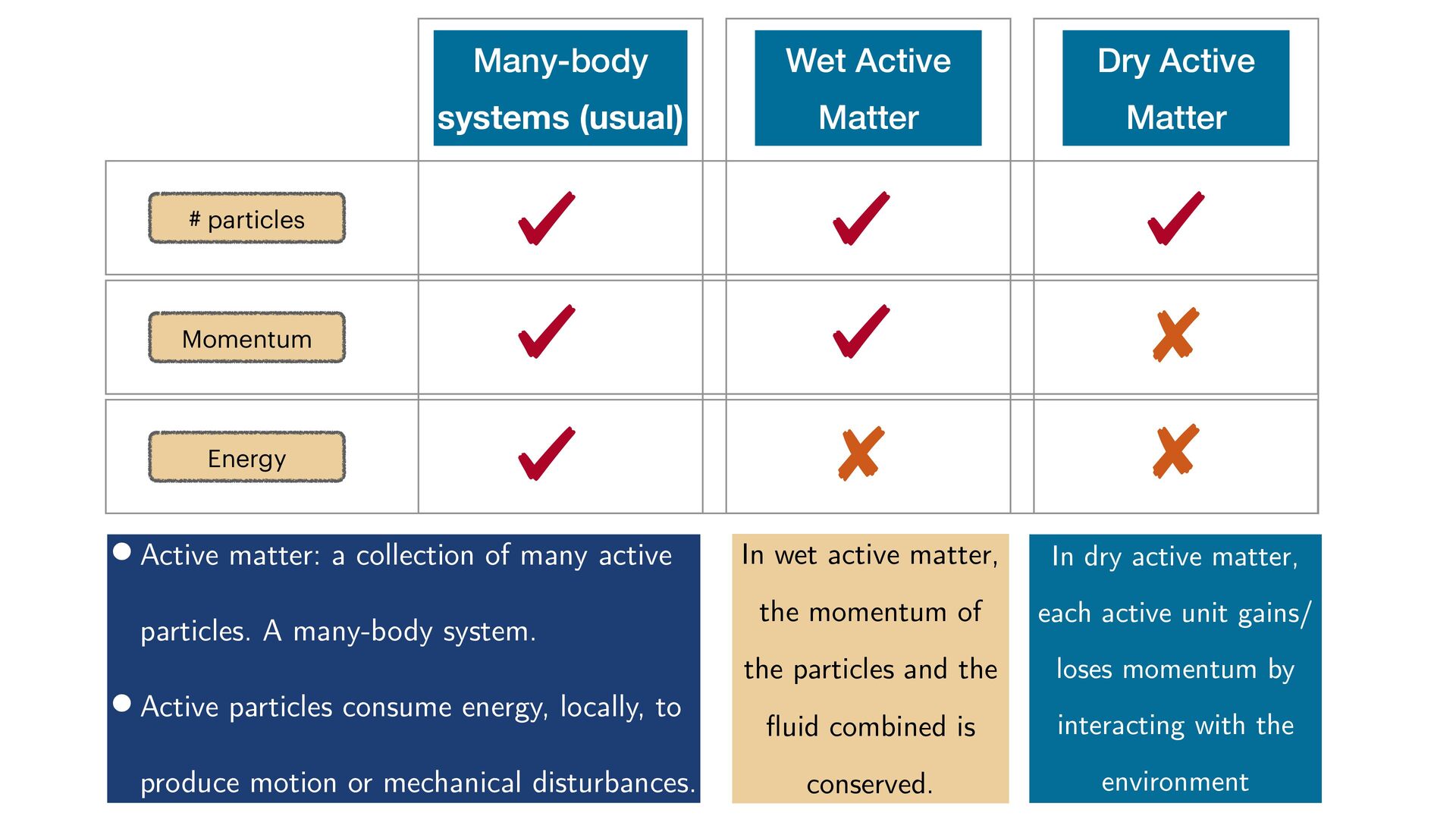
Wet Active Matter In dry active matter, each active unit gains/ loses momentum by interacting with the environment In wet active matter, the momentum of the particles and the fluid combined is conserved. • Active matter: a collection of many active particles. A many-body system. • Active particles consume energy, locally, to produce motion or mechanical disturbances.
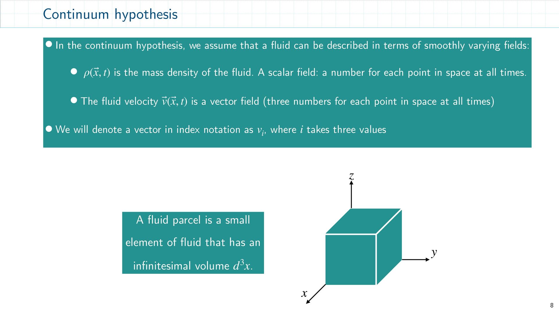
can be described in terms of smoothly varying fields: • is the mass density of the fluid. A scalar field: a number for each point in space at all times. • The fluid velocity is a vector field (three numbers for each point in space at all times) • We will denote a vector in index notation as , where takes three values ρ( ⃗ x, t) ⃗ v( ⃗ x, t) v i i 8 Continuum hypothesis z x y A fluid parcel is a small element of fluid that has an infinitesimal volume . d3x
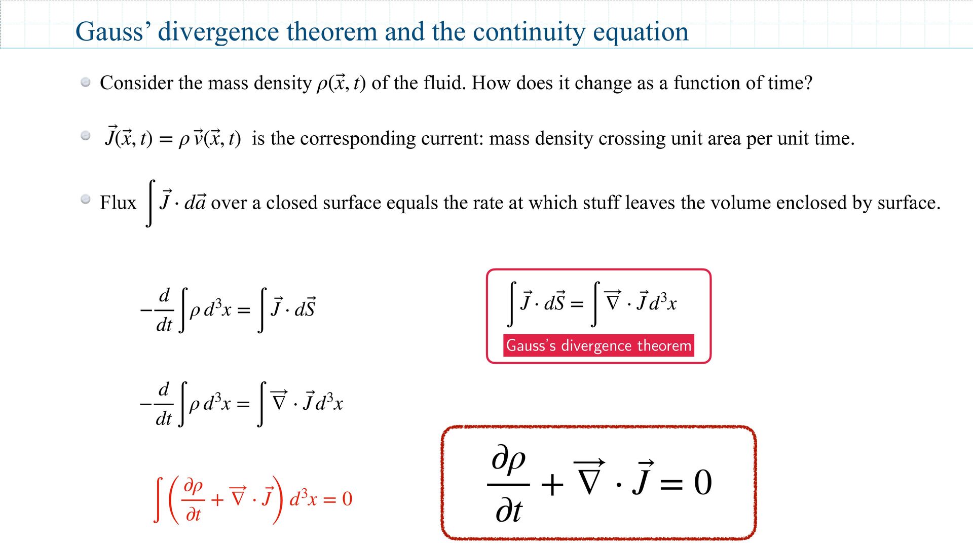
⋅ d ⃗ S − d dt ∫ ρ d3x = ∫ ⃗ ∇ ⋅ ⃗ J d3x ∫ ( ∂ρ ∂t + ⃗ ∇ ⋅ ⃗ J ) d3x = 0 Gauss’ divergence theorem and the continuity equation Consider the mass density of the fluid. How does it change as a function of time? is the corresponding current: mass density crossing unit area per unit time. Flux over a closed surface equals the rate at which stuff leaves the volume enclosed by surface. ρ( ⃗ x, t) ⃗ J( ⃗ x, t) = ρ ⃗ v( ⃗ x, t) ∫ ⃗ J ⋅ d ⃗ a ∂ρ ∂t + ⃗ ∇ ⋅ ⃗ J = 0 ∫ ⃗ J ⋅ d ⃗ S = ∫ ⃗ ∇ ⋅ ⃗ J d3x Gauss’s divergence theorem
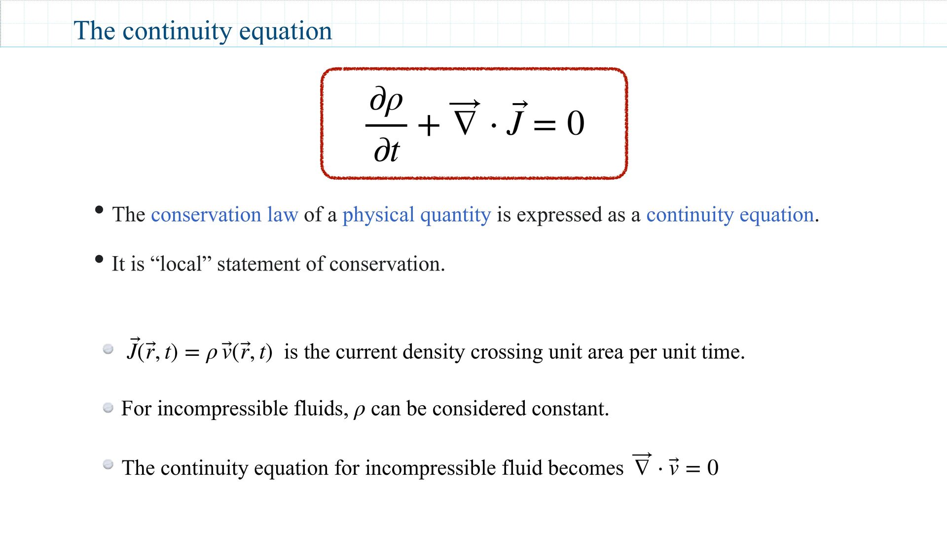
• The conservation law of a physical quantity is expressed as a continuity equation. • It is “local” statement of conservation. The continuity equation is the current density crossing unit area per unit time. For incompressible fluids, can be considered constant. The continuity equation for incompressible fluid becomes ⃗ J( ⃗ r, t) = ρ ⃗ v( ⃗ r, t) ρ ⃗ ∇ ⋅ ⃗ v = 0
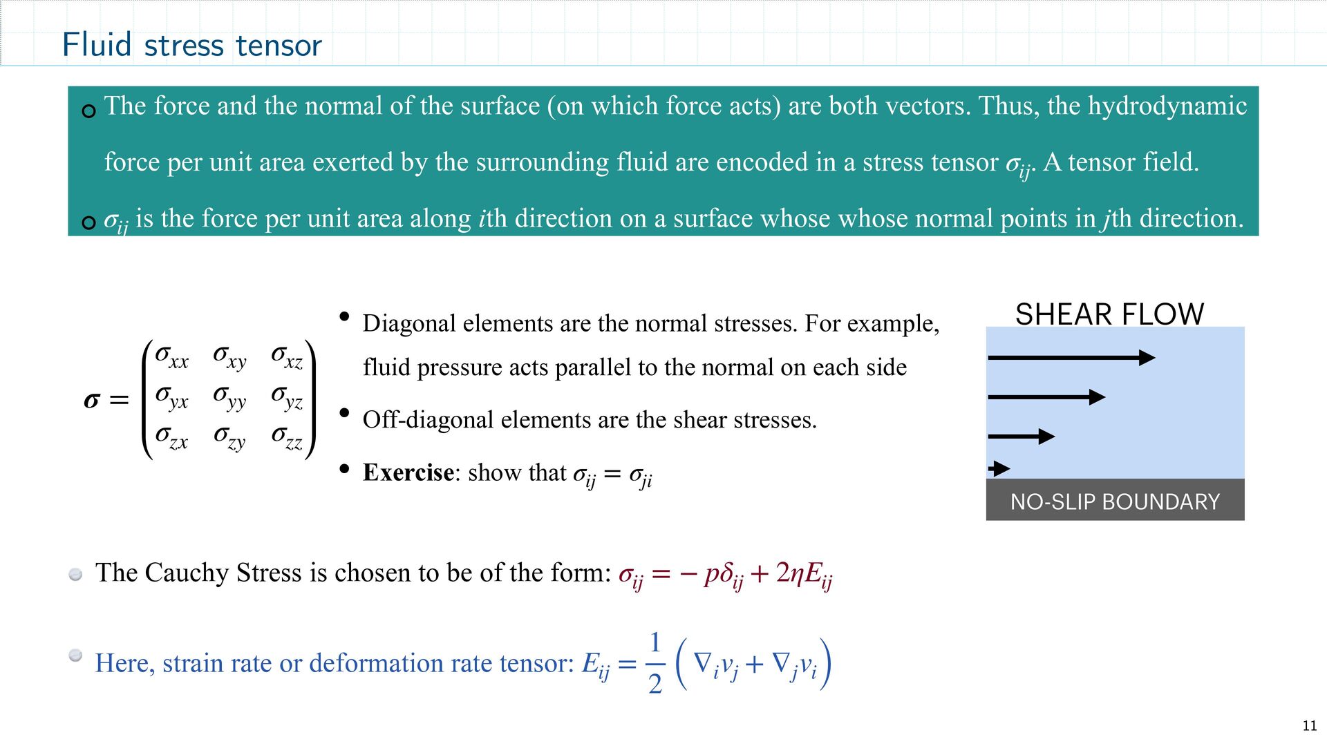
which force acts) are both vectors. Thus, the hydrodynamic force per unit area exerted by the surrounding fluid are encoded in a stress tensor . A tensor field. is the force per unit area along ith direction on a surface whose whose normal points in jth direction. σ ij σ ij Fluid stress tensor The Cauchy Stress is chosen to be of the form: Here, strain rate or deformation rate tensor: σ ij = − pδ ij + 2ηE ij E ij = 1 2 ( ∇ i v j + ∇ j v i) σ = σ xx σ xy σ xz σ yx σ yy σ yz σ zx σ zy σ zz • Diagonal elements are the normal stresses. For example, fluid pressure acts parallel to the normal on each side • Off-diagonal elements are the shear stresses. • Exercise: show that σ ij = σ ji NO-SLIP BOUNDARY SHEAR FLOW
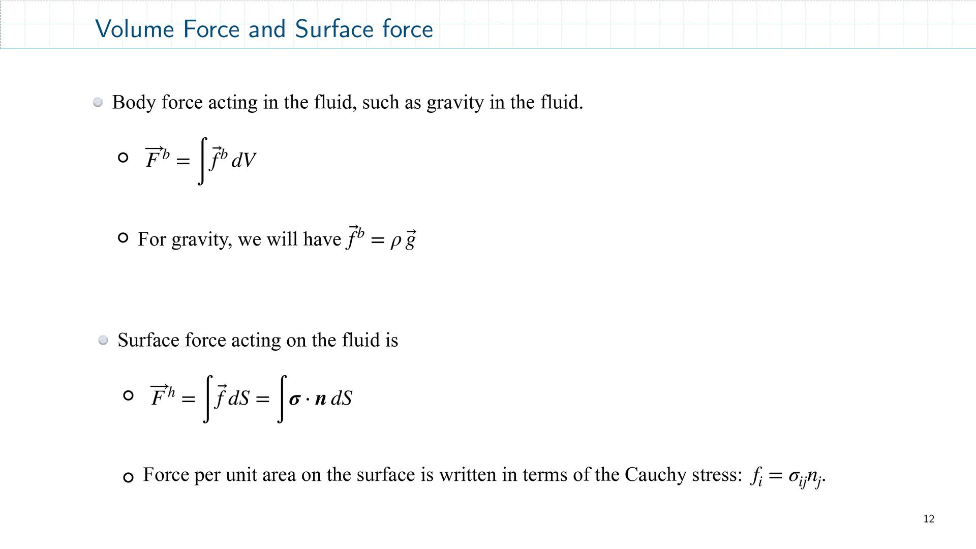
the fluid, such as gravity in the fluid. For gravity, we will have ⃗ F b = ∫ ⃗ fb dV ⃗ fb = ρ ⃗ g Surface force acting on the fluid is Force per unit area on the surface is written in terms of the Cauchy stress: . ⃗ F h = ∫ ⃗ f dS = ∫ σ ⋅ n dS f i = σ ij n j
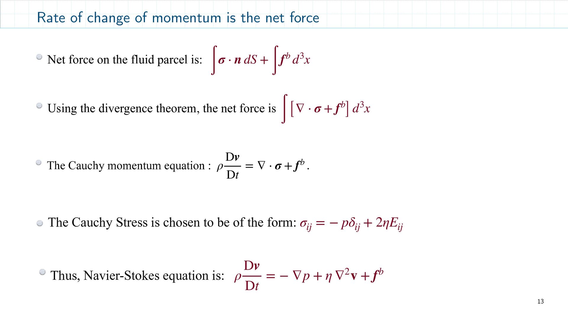
divergence theorem, the net force is ∫ σ ⋅ n dS + ∫ fb d3x ∫ [∇ ⋅ σ + fb ] d3x Rate of change of momentum is the net force The Cauchy momentum equation : ρ Dv Dt = ∇ ⋅ σ + fb . The Cauchy Stress is chosen to be of the form: σ ij = − pδ ij + 2ηE ij Thus, Navier-Stokes equation is: ρ Dv Dt = − ∇p + η ∇2v + fb
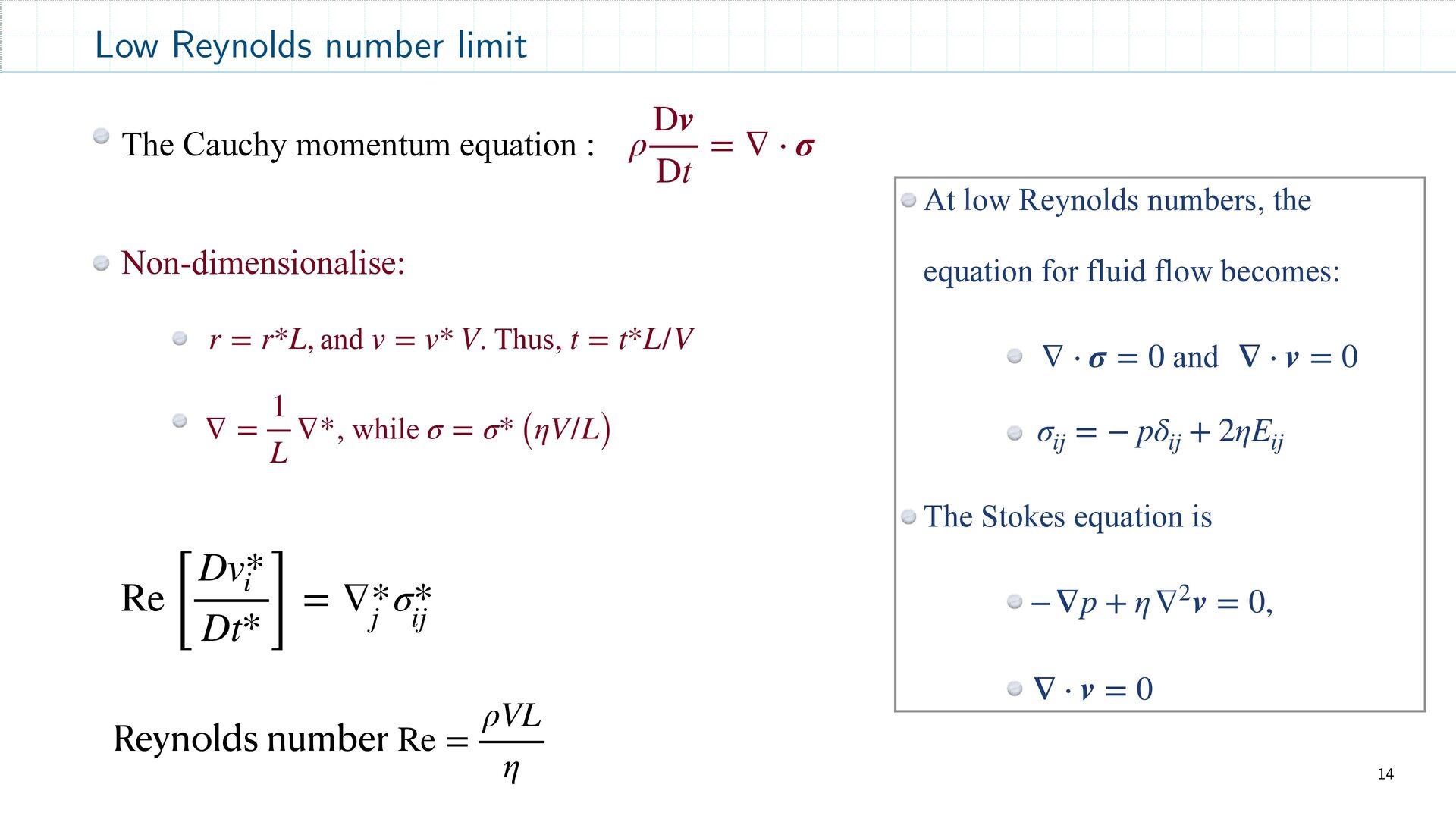
Non-dimensionalise: and . Thus, , while ρ Dv Dt = ∇ ⋅ σ r = r*L, v = v* V t = t*L/V ∇ = 1 L ∇* σ = σ* (ηV/L) Re [ Dv* i Dt* ] = ∇* j σ* ij Reynolds number Re = ρVL η At low Reynolds numbers, the equation for fluid flow becomes: and The Stokes equation is ∇ ⋅ σ = 0 ∇ ⋅ v = 0 σ ij = − pδ ij + 2ηE ij −∇p + η∇2v = 0, ∇ ⋅ v = 0
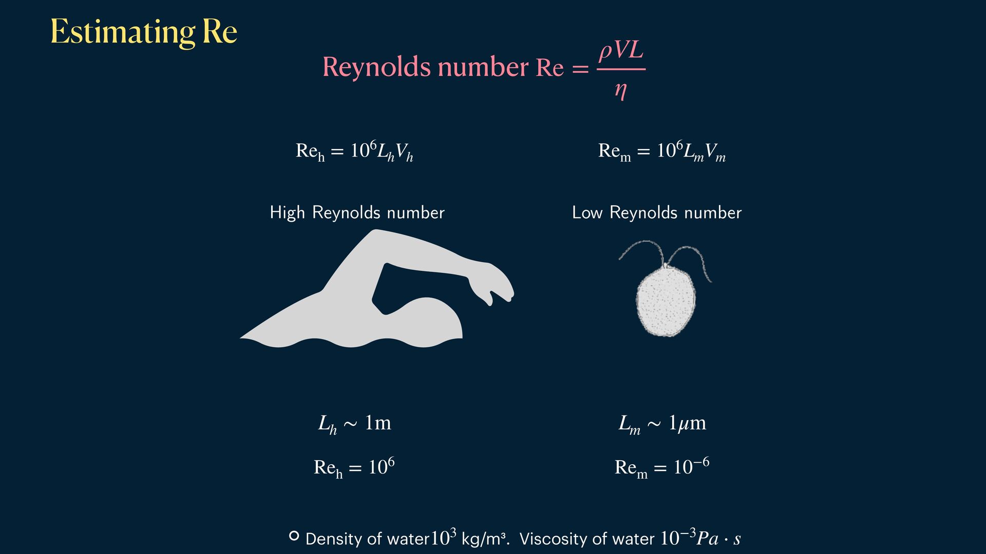
number Low Reynolds number L h ∼ 1m L m ∼ 1μm 15 Estimating Re Reynolds number Re = ρVL η Re h = 106L h V h Re m = 106L m V m Density of water kg/m³. Viscosity of water 103 10−3Pa ⋅ s
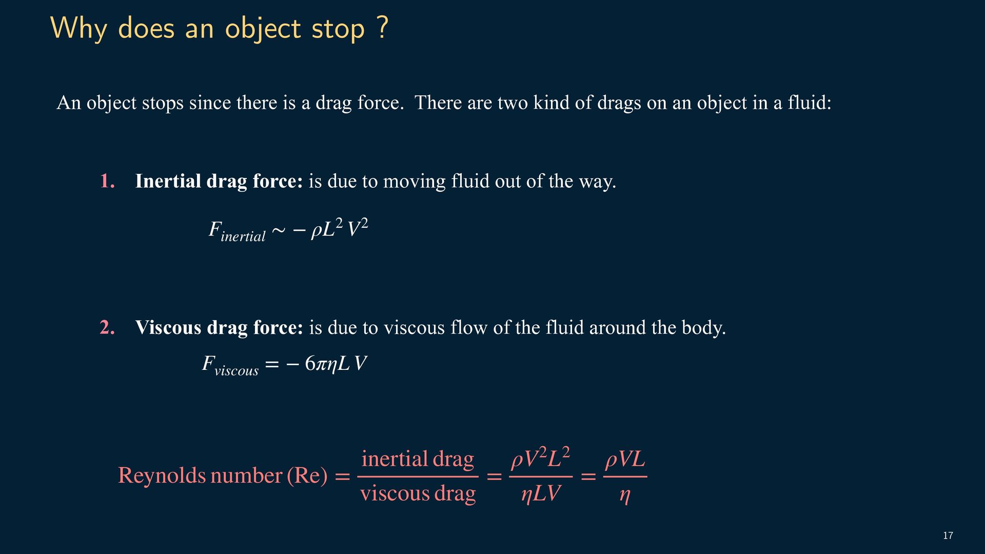
there is a drag force. There are two kind of drags on an object in a fluid: 17 1. Inertial drag force: is due to moving fluid out of the way. 2. Viscous drag force: is due to viscous flow of the fluid around the body. F inertial ∼ − ρL2 V2 F viscous = − 6πηL V Reynolds number (Re) = inertial drag viscous drag = ρV2L2 ηLV = ρVL η
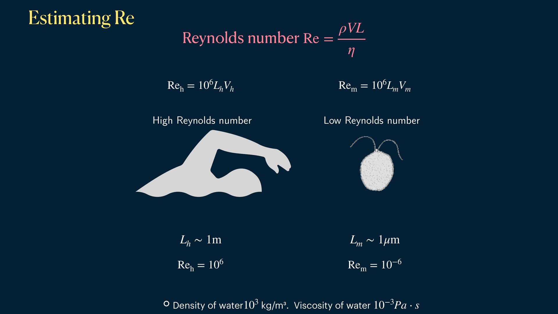
number Low Reynolds number L h ∼ 1m L m ∼ 1μm 18 Estimating Re Reynolds number Re = ρVL η Re h = 106L h V h Re m = 106L m V m Density of water kg/m³. Viscosity of water 103 10−3Pa ⋅ s
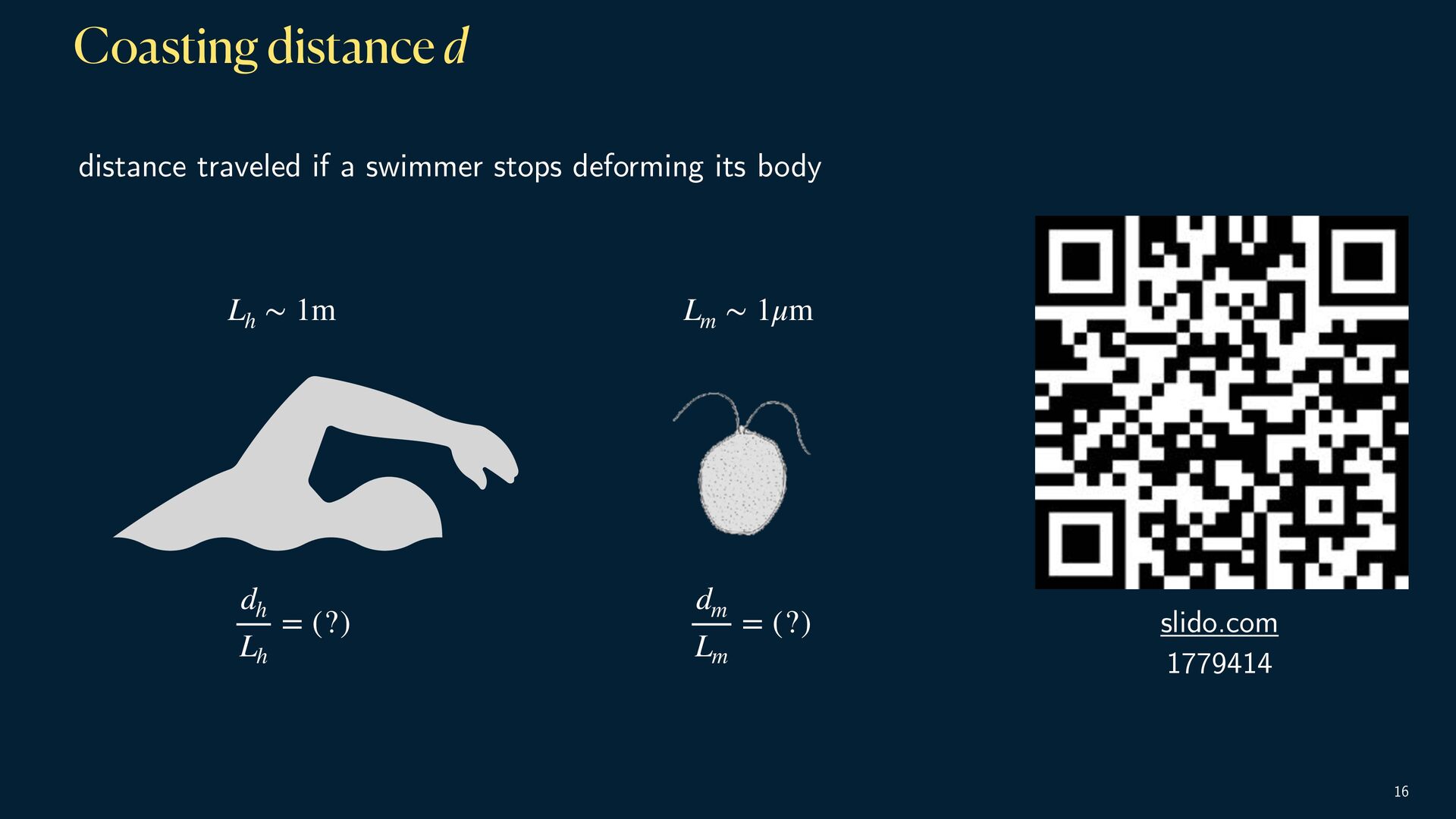
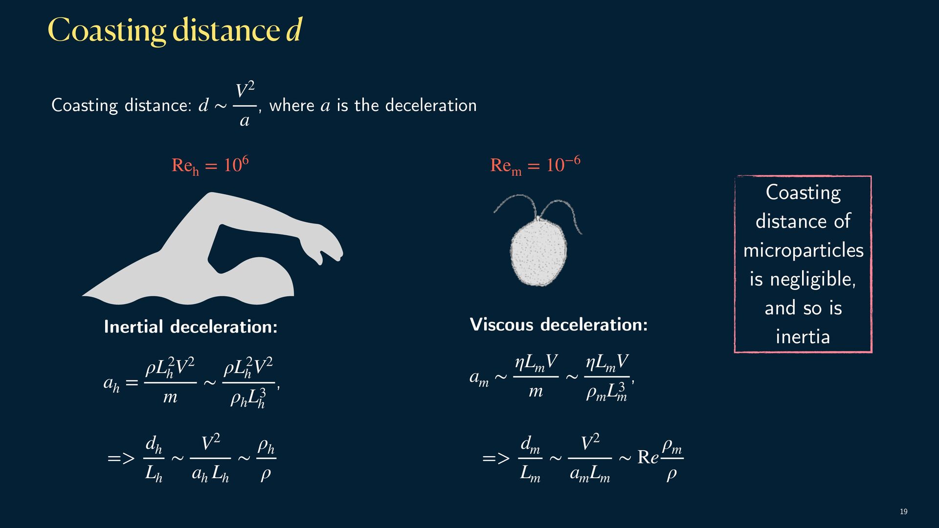
h V2 m ∼ ρL2 h V2 ρh L3 h Coasting distance: , where is the deceleration d ∼ V2 a a Viscous deceleration: , a m ∼ ηL m V m ∼ ηL m V ρm L3 m Coasting distance of microparticles is negligible, and so is inertia Re h = 106 Re m = 10−6 Coasting distance d => d h Lh ∼ V2 ah Lh ∼ ρ h ρ => d m Lm ∼ V2 am Lm ∼ Re ρ m ρ
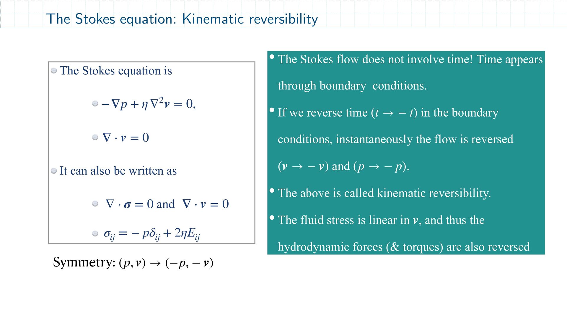
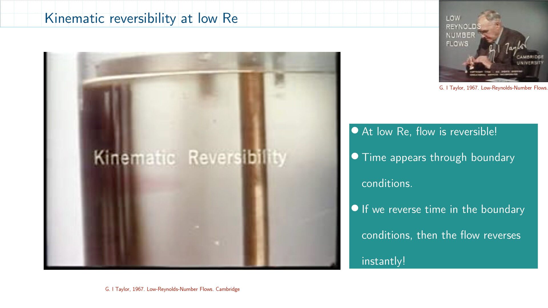
involve time! Time appears through boundary conditions. •If we reverse time in the boundary conditions, instantaneously the flow is reversed and . •The above is called kinematic reversibility. •The fluid stress is linear in , and thus the hydrodynamic forces (& torques) are also reversed (t → − t) (v → − v) (p → − p) v Symmetry: (p, v) → (−p, − v) The Stokes equation is It can also be written as and −∇p + η∇2v = 0, ∇ ⋅ v = 0 ∇ ⋅ σ = 0 ∇ ⋅ v = 0 σ ij = − pδ ij + 2ηE ij
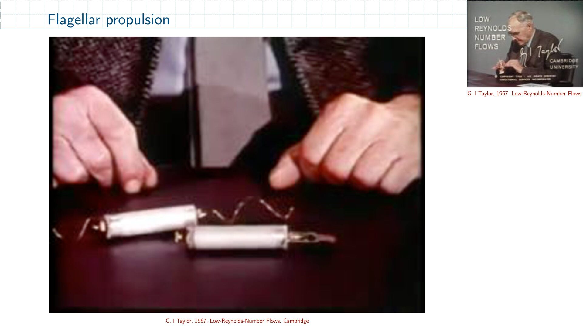
is reversible! • Time appears through boundary conditions. • If we reverse time in the boundary conditions, then the flow reverses instantly! G. I Taylor, 1967. Low-Reynolds-Number Flows. Cambridge G. I Taylor, 1967. Low-Reynolds-Number Flows.
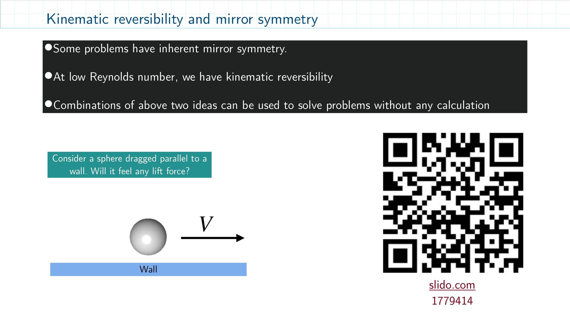
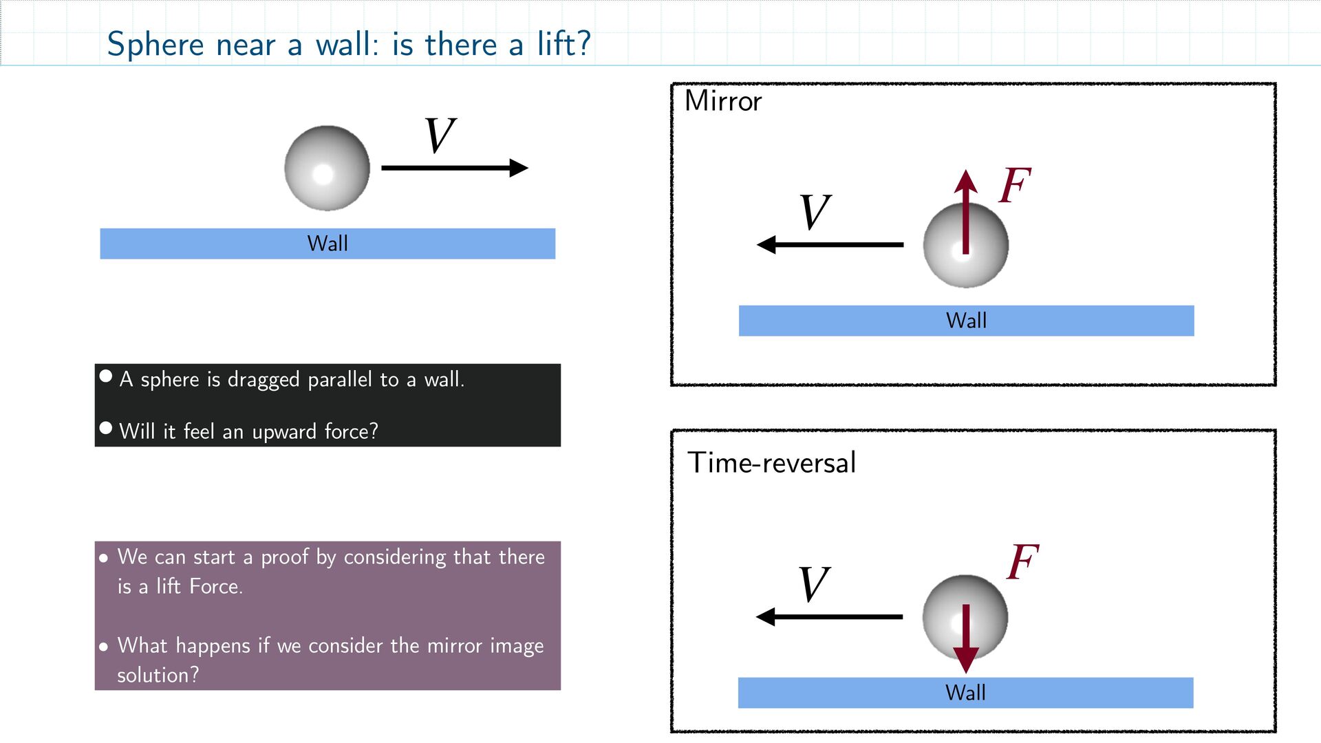
symmetry. •At low Reynolds number, we have kinematic reversibility •Combinations of above two ideas can be used to solve problems without any calculation Wall V slido.com 1779414 Consider a sphere dragged parallel to a wall. Will it feel any lift force?
• A sphere is dragged parallel to a wall. • Will it feel an upward force? Time-reversal Wall V F Mirror Wall V F • We can start a proof by considering that there is a lift Force. • What happens if we consider the mirror image solution?
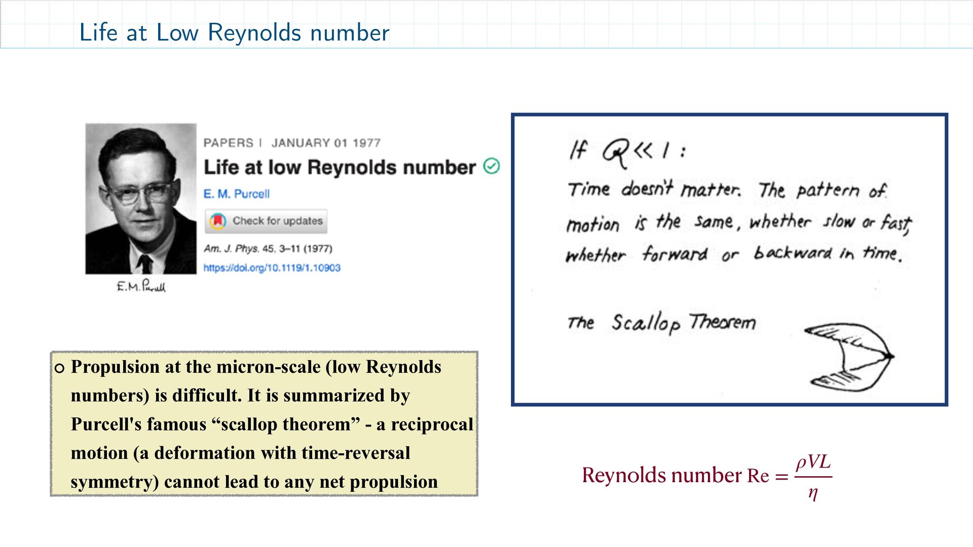
η Propulsion at the micron-scale (low Reynolds numbers) is difficult. It is summarized by Purcell's famous “scallop theorem” - a reciprocal motion (a deformation with time-reversal symmetry) cannot lead to any net propulsion
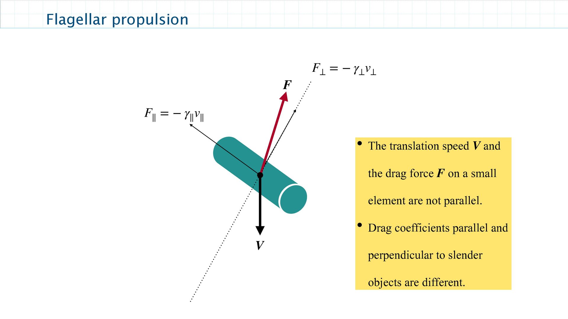
∥ F ⊥ = − γ ⊥ v ⊥ F • The translation speed and the drag force on a small element are not parallel. • Drag coefficients parallel and perpendicular to slender objects are different. V F
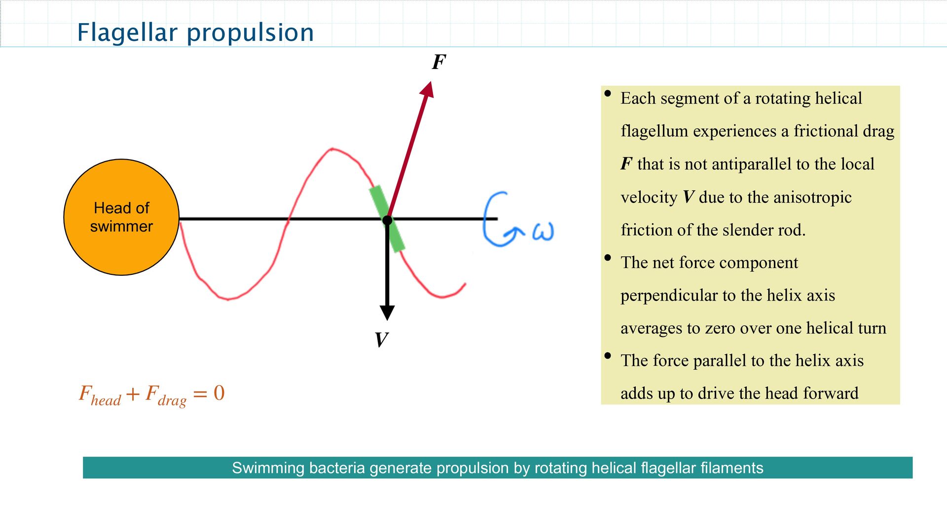
filaments • Each segment of a rotating helical flagellum experiences a frictional drag that is not antiparallel to the local velocity due to the anisotropic friction of the slender rod. • The net force component perpendicular to the helix axis averages to zero over one helical turn • The force parallel to the helix axis adds up to drive the head forward F V V F Head of swimmer F head + F drag = 0
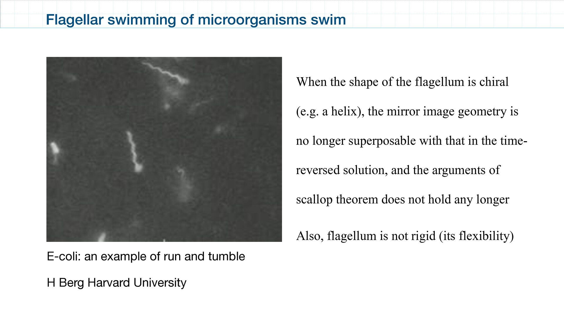
University When the shape of the flagellum is chiral (e.g. a helix), the mirror image geometry is no longer superposable with that in the time- reversed solution, and the arguments of scallop theorem does not hold any longer Also, flagellum is not rigid (its flexibility) Flagellar swimming of microorganisms swim
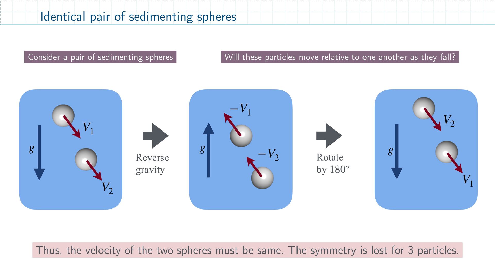
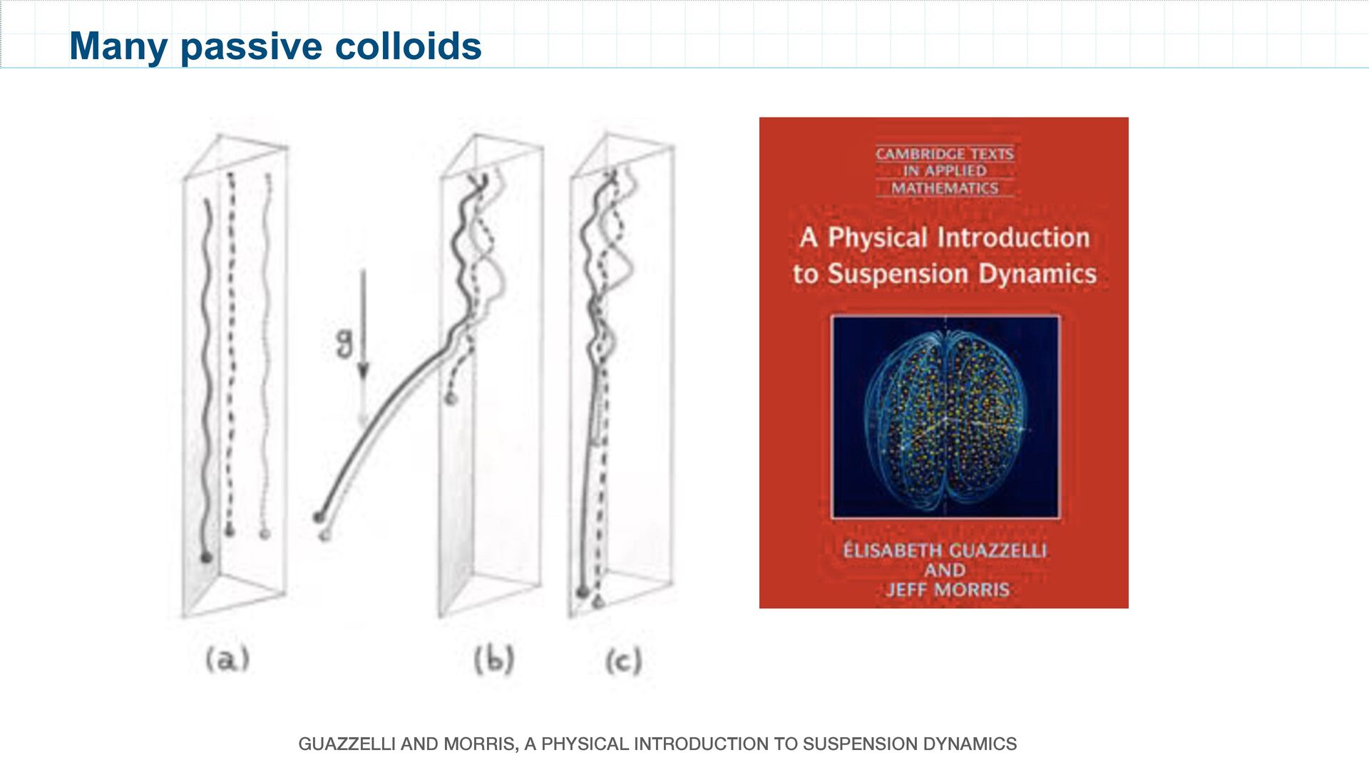
to one another as they fall? Thus, the velocity of the two spheres must be same. The symmetry is lost for 3 particles. Consider a pair of sedimenting spheres g V 1 V 2 g −V 1 −V 2 g V 2 V 1 Reverse gravity Rotate by 180o
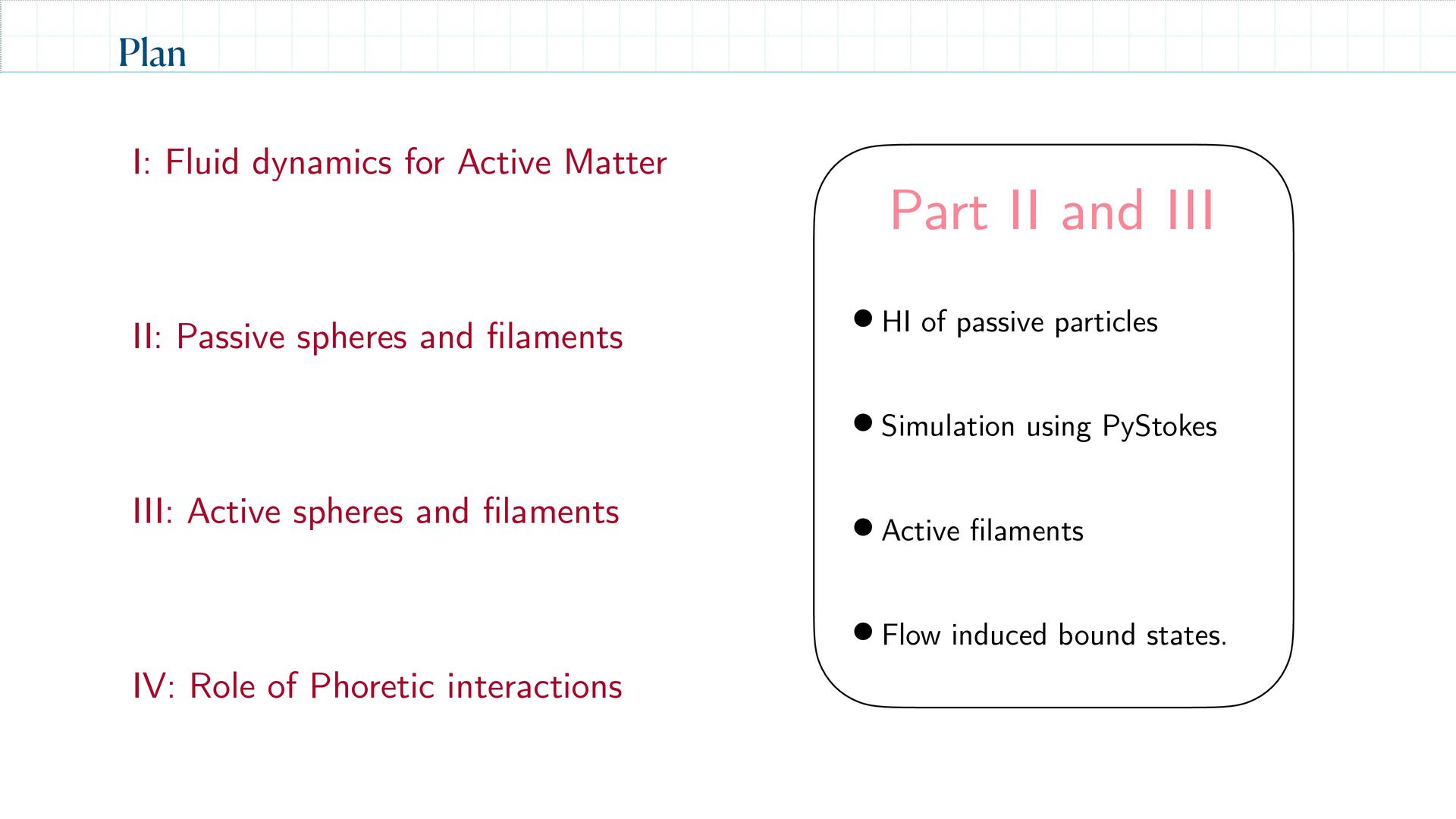
PyStokes • Active filaments • Flow induced bound states. Part II and III I: Fluid dynamics for Active Matter II: Passive spheres and filaments IV: Role of Phoretic interactions III: Active spheres and filaments
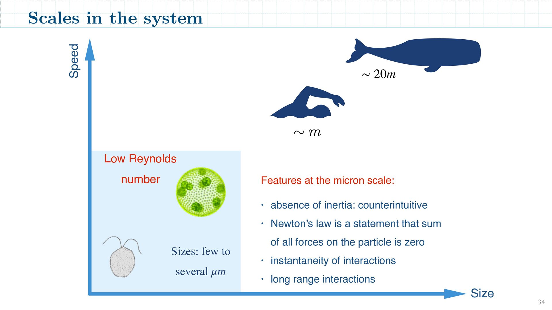
• absence of inertia: counterintuitive • Newton’s law is a statement that sum of all forces on the particle is zero • instantaneity of interactions • long range interactions Scales in the system ∼ 20m Low Reynolds number Sizes: few to several μm
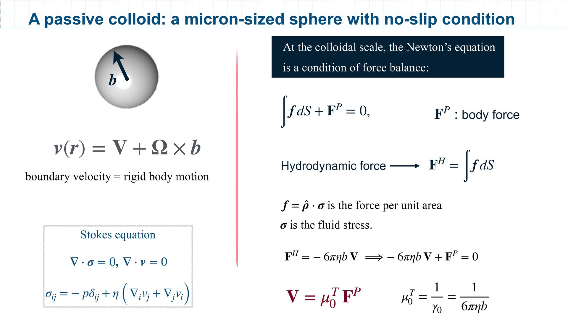
micron-sized sphere with no-slip condition v(r) = V + Ω × b Stokes equation , ∇ ⋅ σ = 0 ∇ ⋅ v = 0 σ ij = − pδ ij + η ( ∇ i v j + ∇ j v i) b body force FP : ∫ f dS + FP = 0, is the force per unit area is the fluid stress. f = ̂ ρ ⋅ σ σ FH = ∫ f dS Hydrodynamic force At the colloidal scale, the Newton’s equation is a condition of force balance: FH = − 6πηb V ⟹ − 6πηb V + FP = 0 V = μT 0 FP μT 0 = 1 γ0 = 1 6πηb
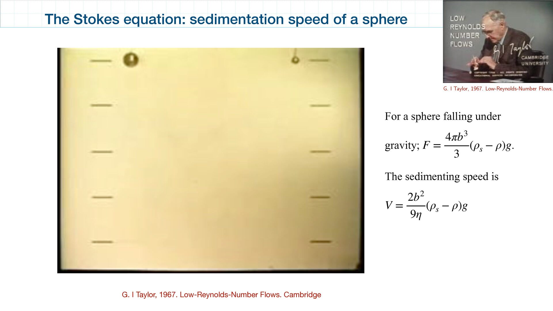
sedimentation speed of a sphere For a sphere falling under gravity; . The sedimenting speed is F = 4πb3 3 (ρ s − ρ)g V = 2b2 9η (ρ s − ρ)g G. I Taylor, 1967. Low-Reynolds-Number Flows.
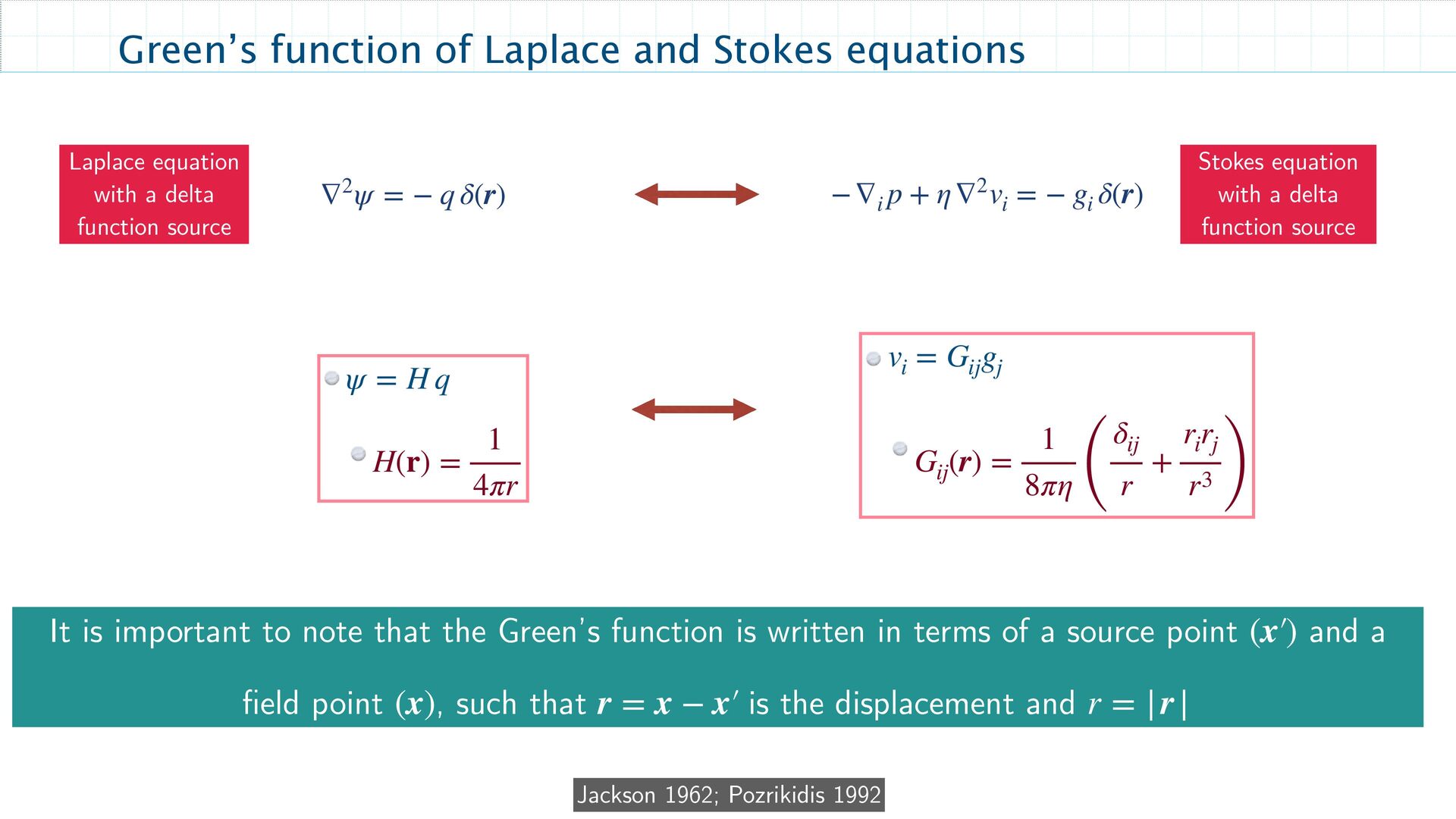
source Stokes equation with a delta function source −∇ i p + η∇2v i = − g i δ(r) ∇2ψ = − q δ(r) Green’s function of Laplace and Stokes equations v i = G ij g j G ij (r) = 1 8πη ( δ ij r + r i r j r3 ) ψ = H q H(r) = 1 4πr It is important to note that the Green’s function is written in terms of a source point and a field point , such that is the displacement and (x′ ) (x) r = x − x′ r = |r|
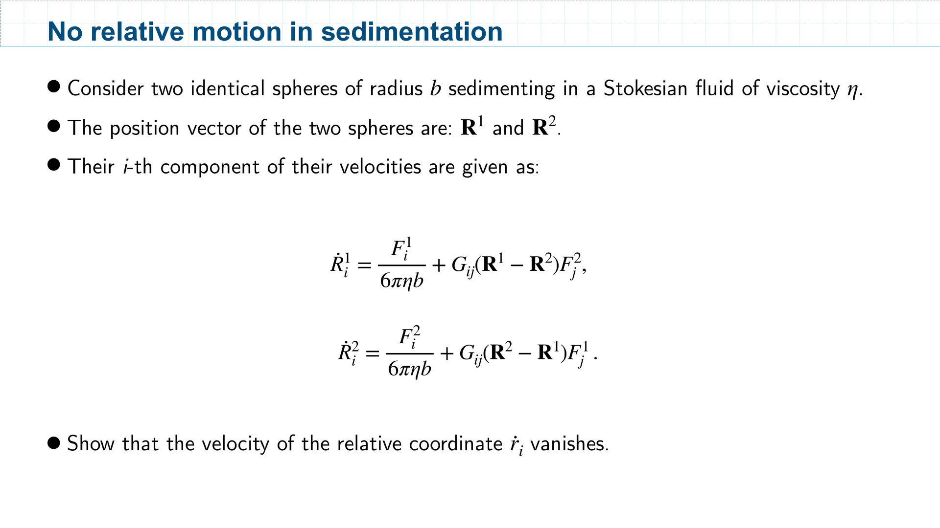
of radius sedimenting in a Stokesian fluid of viscosity . • The position vector of the two spheres are: and . • Their i-th component of their velocities are given as: b η R1 R2 · R1 i = F1 i 6πηb + G ij (R1 − R2)F2 j , · R2 i = F2 i 6πηb + G ij (R2 − R1)F1 j . • Show that the velocity of the relative coordinate vanishes. · r i
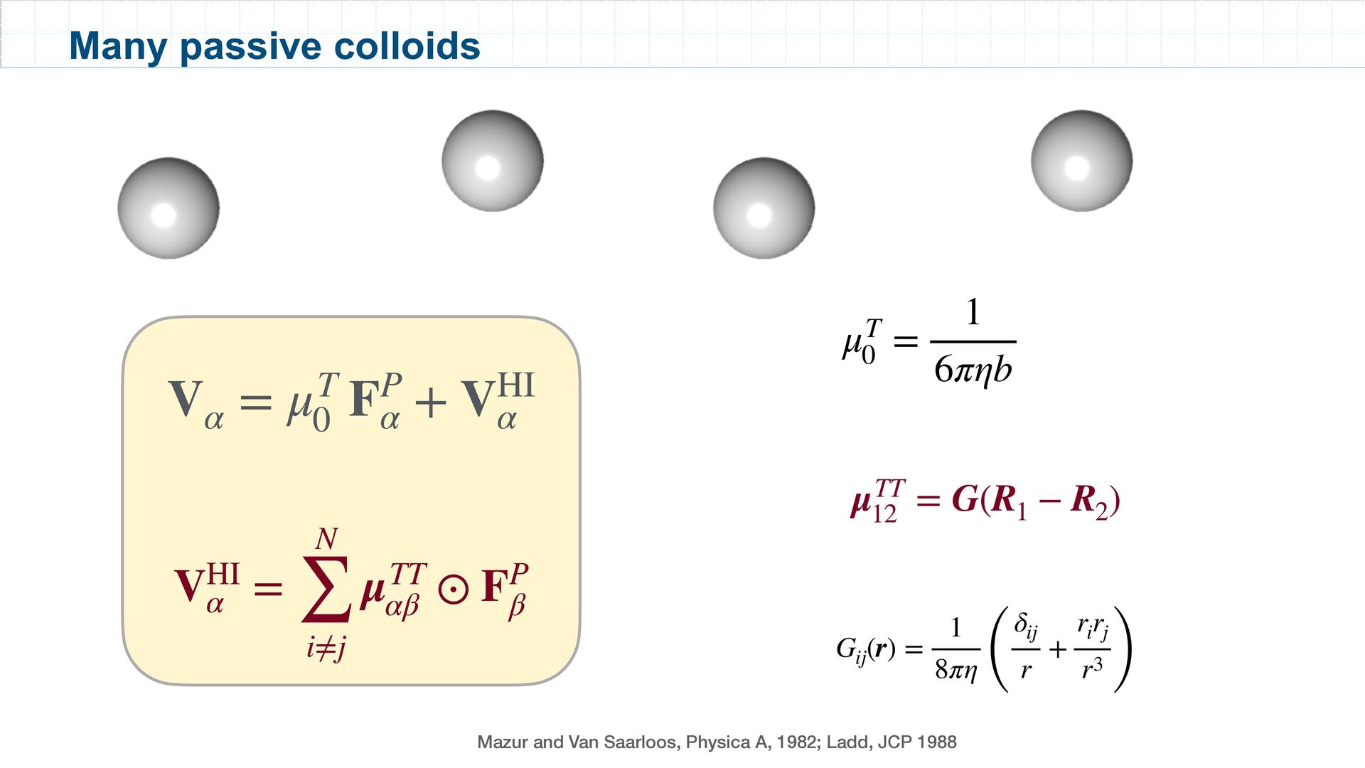
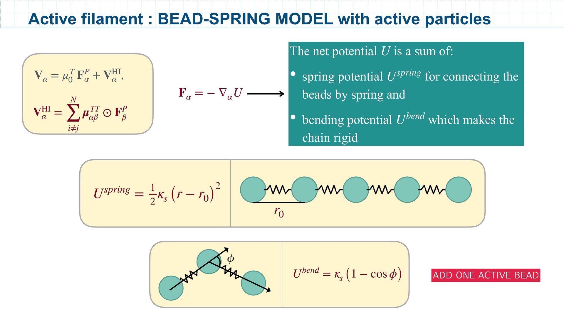
= G(R1 − R2 ) V α = μT 0 FP α + VHI α VHI α = N ∑ i≠j μTT αβ ⊙ FP β Mazur and Van Saarloos, Physica A, 1982; Ladd, JCP 1988 G ij (r) = 1 8πη ( δ ij r + r i r j r3 )
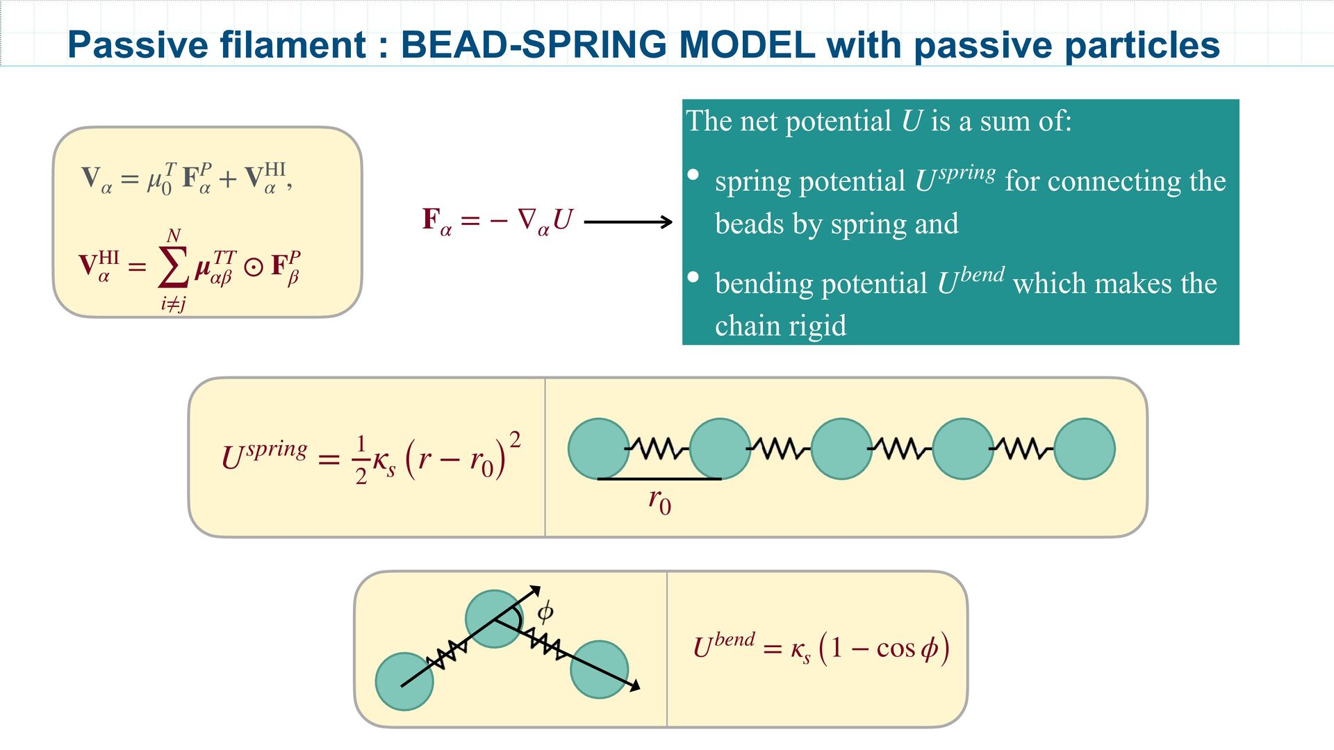
= μT 0 FP α + VHI α , VHI α = N ∑ i≠j μTT αβ ⊙ FP β F α = − ∇ α U The net potential is a sum of: • spring potential for connecting the beads by spring and • bending potential which makes the chain rigid U Uspring Ubend r 0 Uspring = 1 2 κ s (r − r 0) 2 Ubend = κ s (1 − cos ϕ)
Deformation and Orientation of a Microscopic Elastic Filament M. Cosentino Lagomarsino, I. Pagonabarraga, C. P. Lowe https://github.com/rajeshrinet/ismc Demo using PyStokes for simulating the dynamics See Example 03
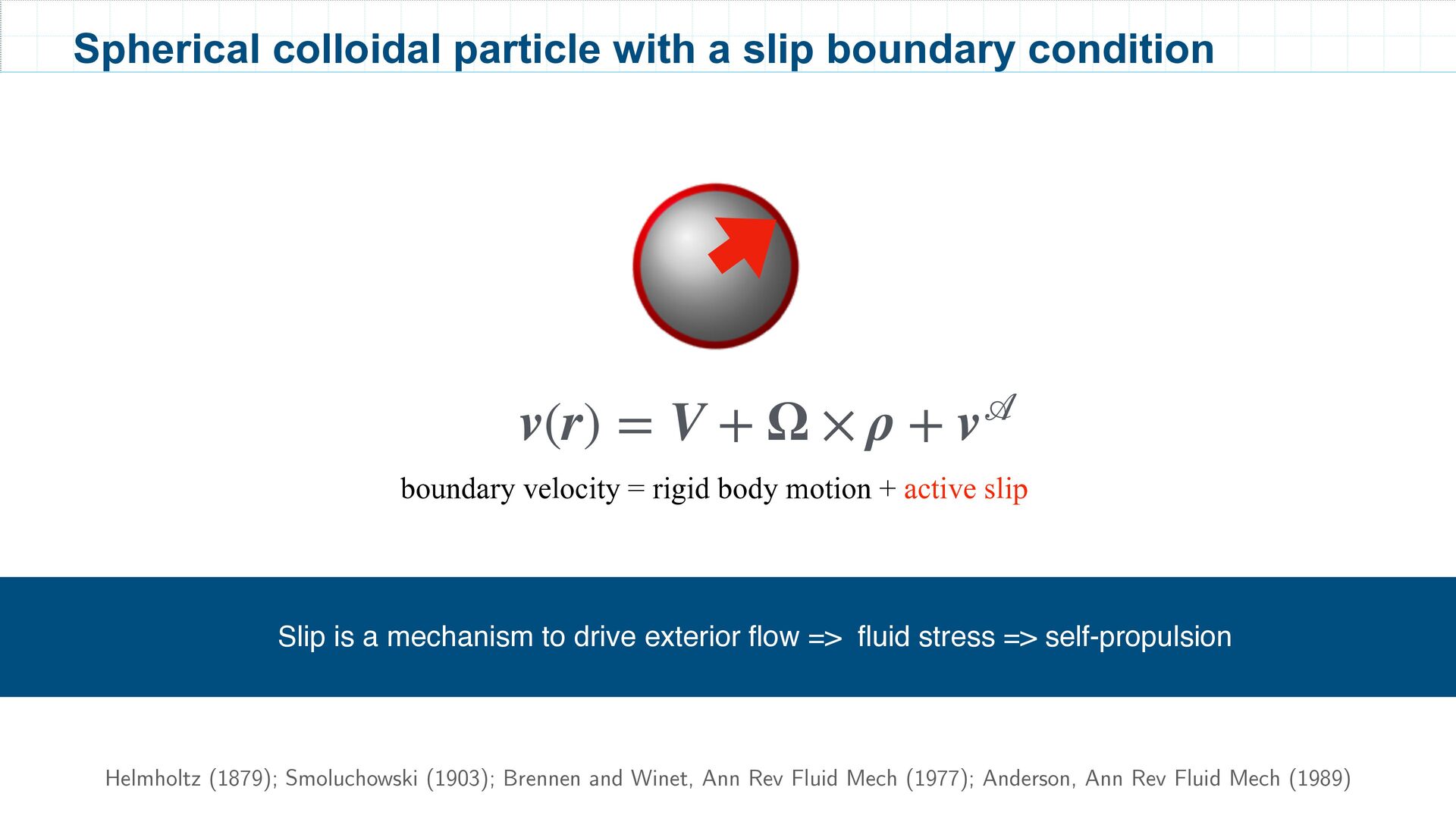
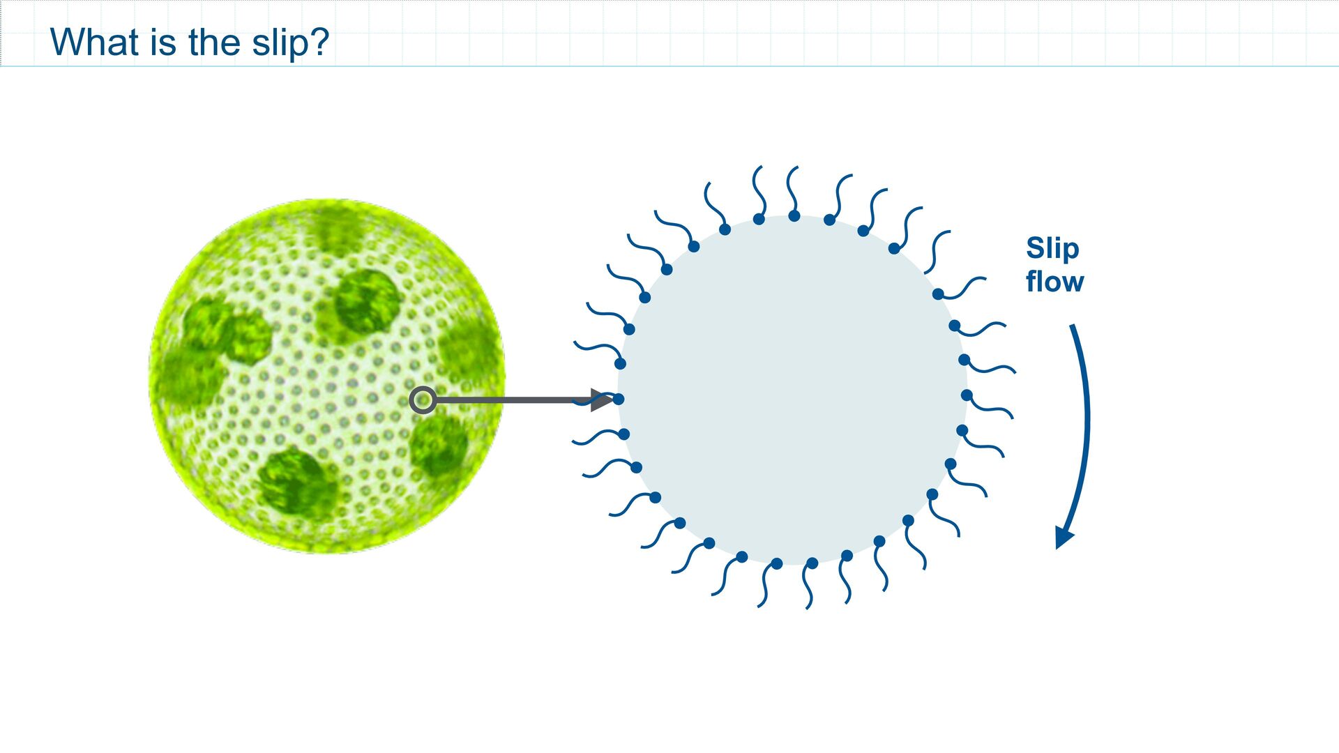
(1879); Smoluchowski (1903); Brennen and Winet, Ann Rev Fluid Mech (1977); Anderson, Ann Rev Fluid Mech (1989) Slip is a mechanism to drive exterior flow => fluid stress => self-propulsion Spherical colloidal particle with a slip boundary condition v(r) = V + Ω × ρ + v
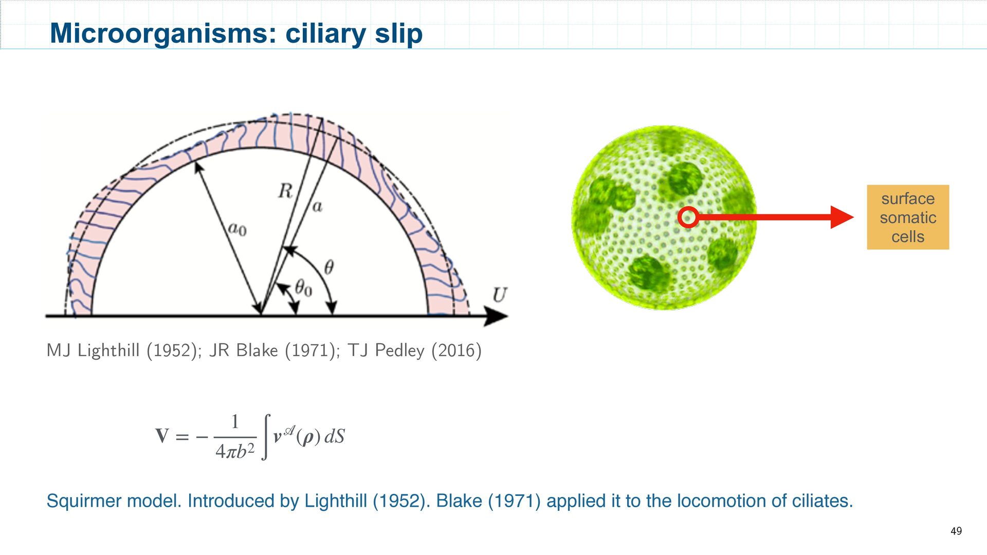
Squirmer model. Introduced by Lighthill (1952). Blake (1971) applied it to the locomotion of ciliates. Microorganisms: ciliary slip V = − 1 4πb2 ∫ v (ρ) dS Top-view of Volvox, a green alga surface somatic cells
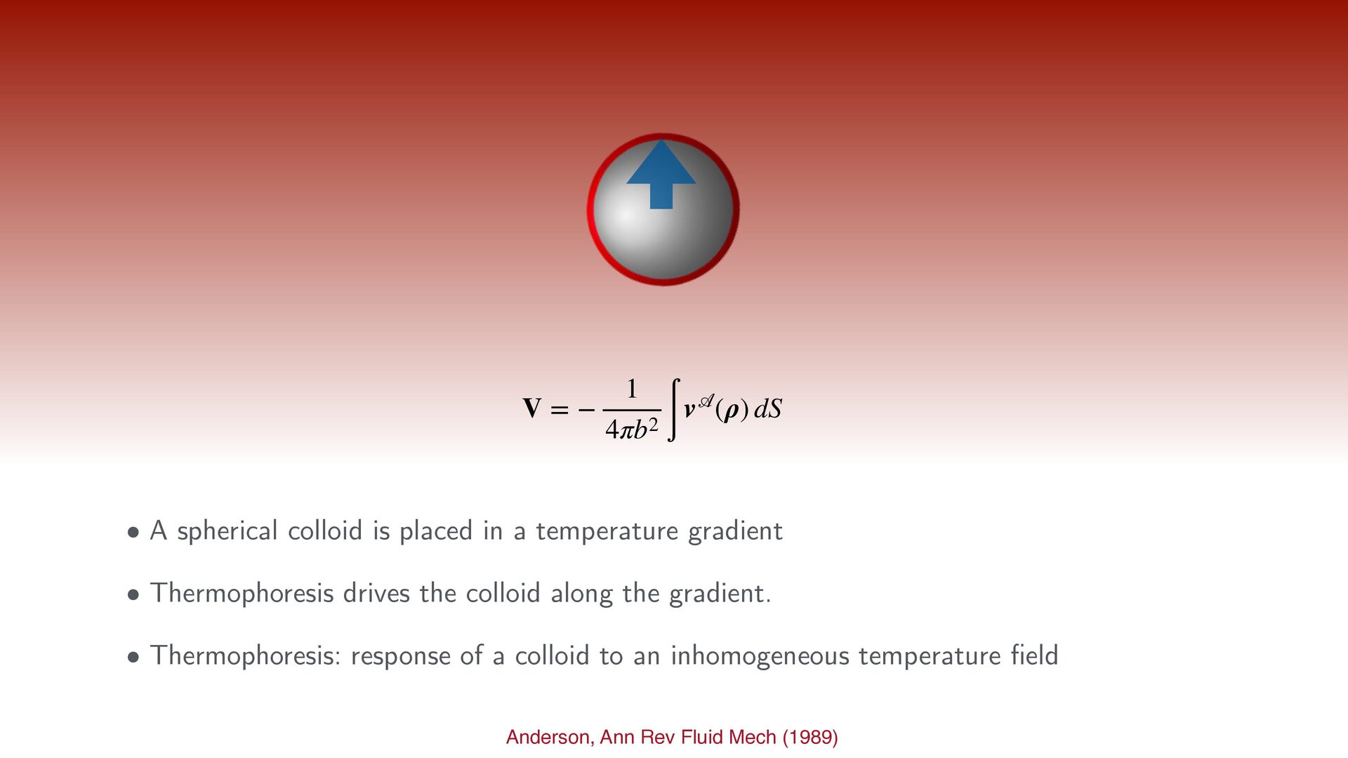
is placed in a temperature gradient • Thermophoresis drives the colloid along the gradient. • Thermophoresis: response of a colloid to an inhomogeneous temperature field V = − 1 4πb2 ∫ v (ρ) dS
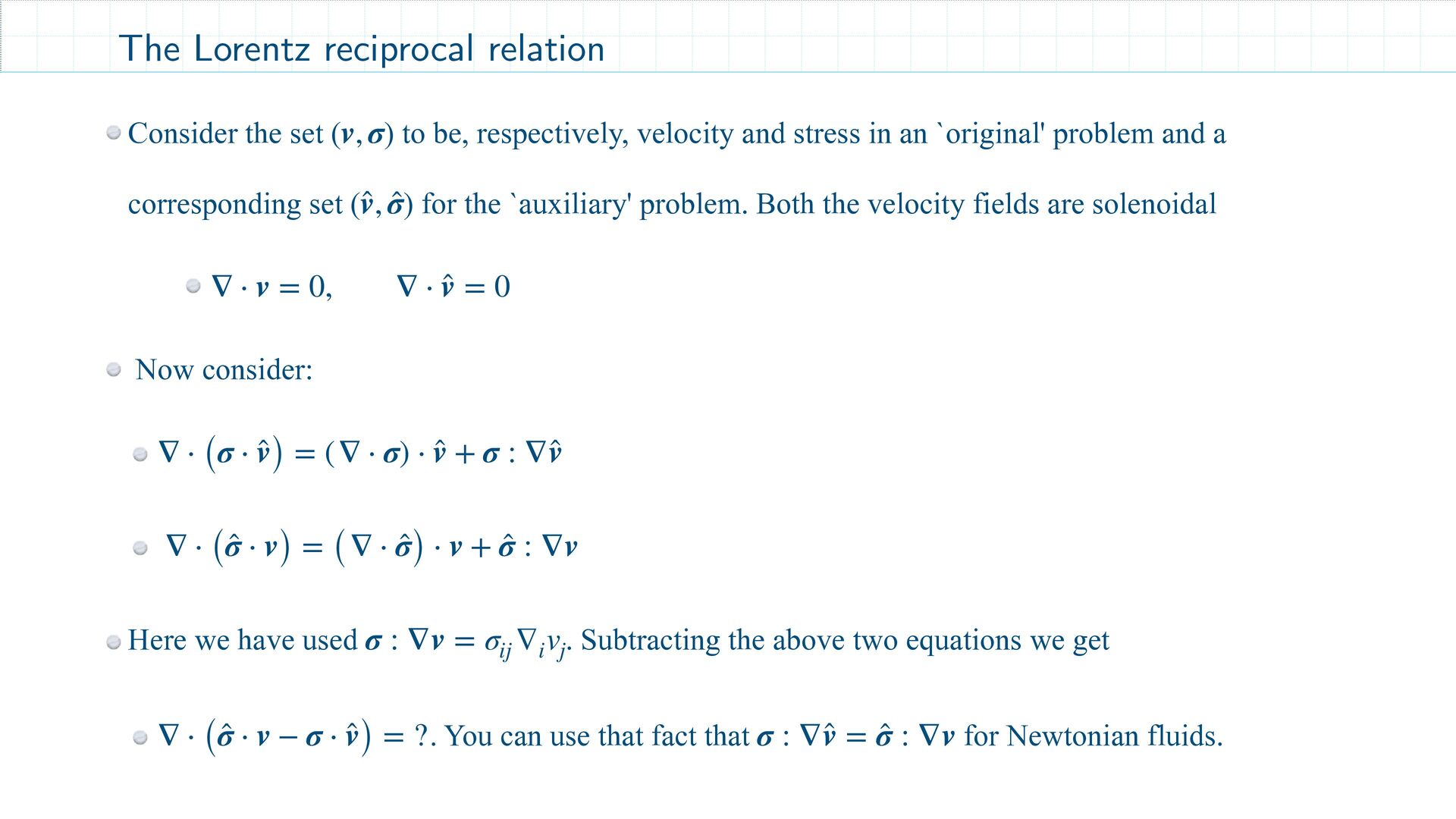
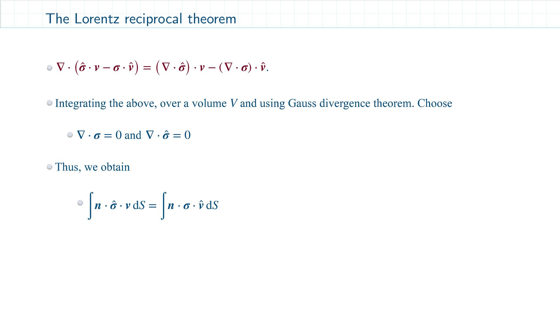
stress in an `original' problem and a corresponding set ( ) for the `auxiliary' problem. Both the velocity fields are solenoidal Now consider: Here we have used . Subtracting the above two equations we get . You can use that fact that for Newtonian fluids. v, σ ̂ v, ̂ σ ∇ ⋅ v = 0, ∇ ⋅ ̂ v = 0 ∇ ⋅ (σ ⋅ ̂ v) = (∇ ⋅ σ) ⋅ ̂ v + σ : ∇ ̂ v ∇ ⋅ ( ̂ σ ⋅ v) = (∇ ⋅ ̂ σ) ⋅ v + ̂ σ : ∇v σ : ∇v = σ ij ∇ i v j ∇ ⋅ ( ̂ σ ⋅ v − σ ⋅ ̂ v) = ? σ : ∇ ̂ v = ̂ σ : ∇v The Lorentz reciprocal relation
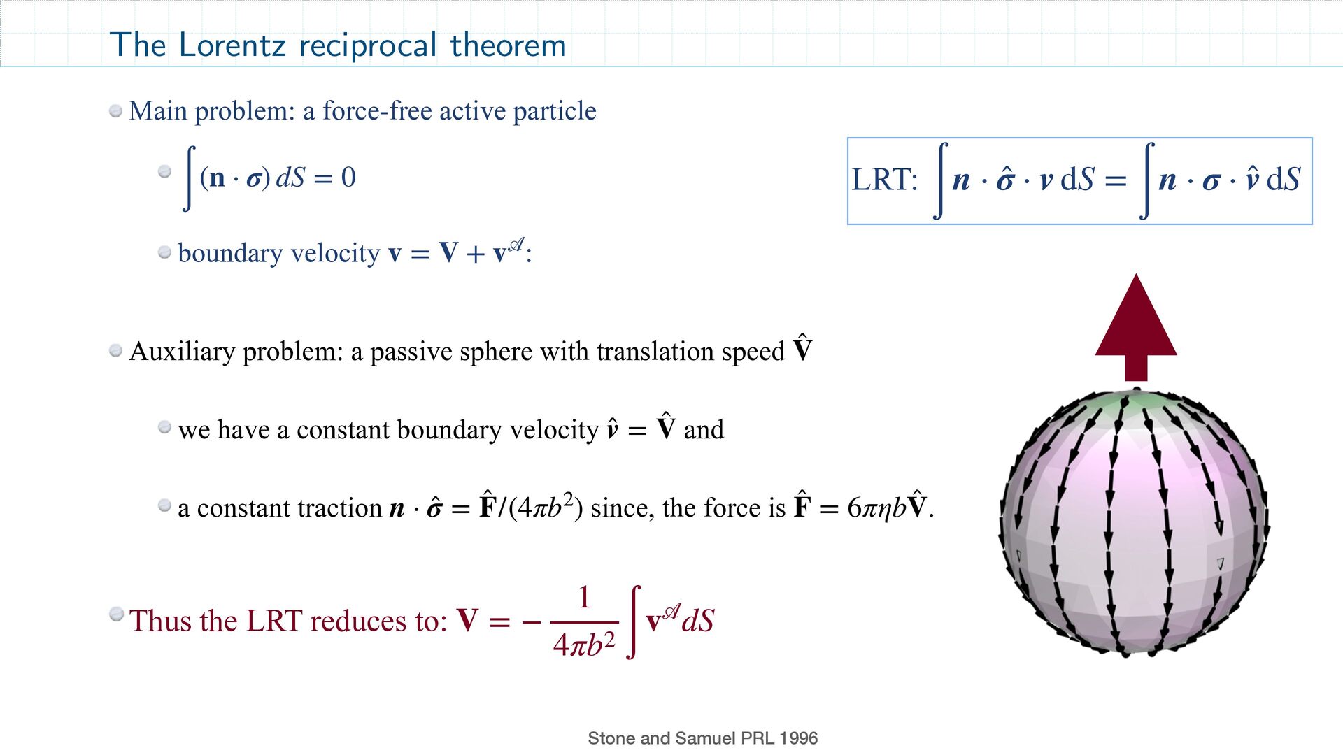
∫ n ⋅ σ ⋅ ̂ v dS The Lorentz reciprocal theorem Main problem: a force-free active particle boundary velocity : ∫ (n ⋅ σ) dS = 0 v = V + v Stone and Samuel PRL 1996 Auxiliary problem: a passive sphere with translation speed we have a constant boundary velocity and a constant traction since, the force is . ̂ V ̂ v = ̂ V n ⋅ ̂ σ = ̂ F/(4πb2) ̂ F = 6πηb ̂ V Thus the LRT reduces to: V = − 1 4πb2 ∫ v dS
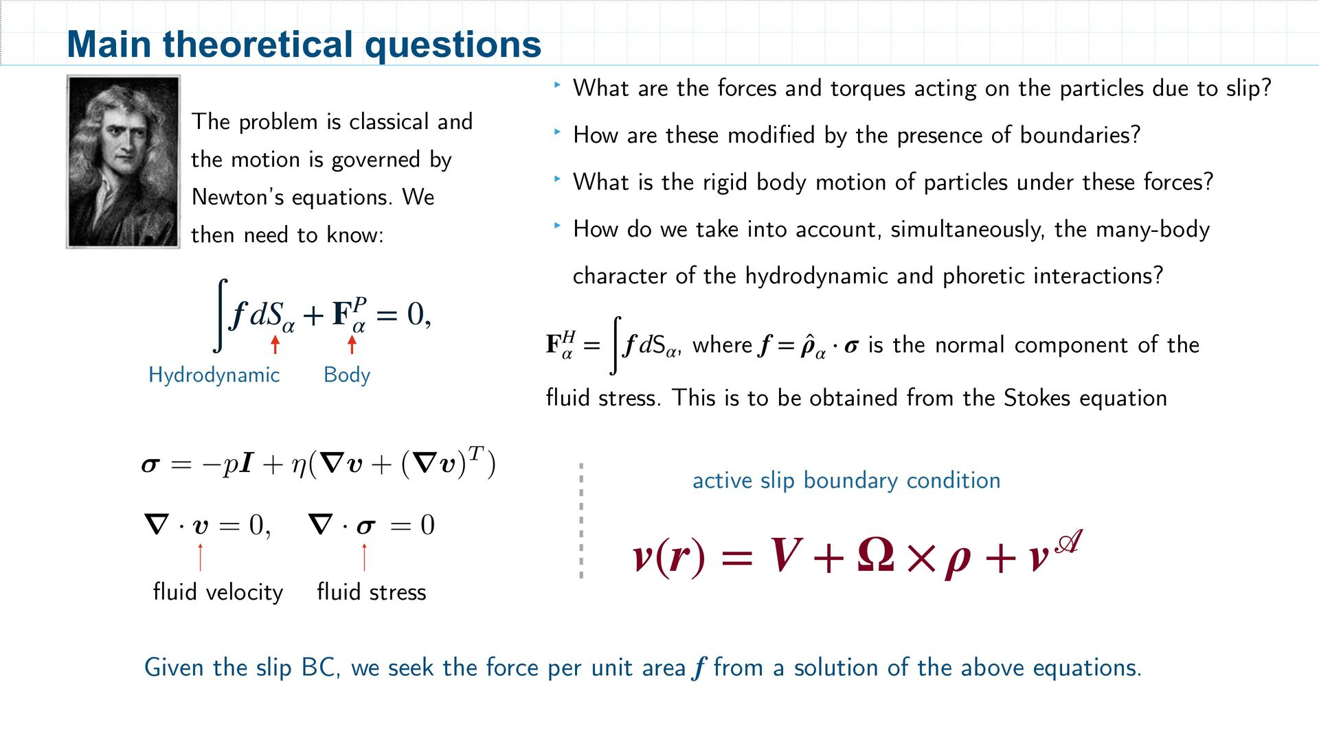
Newton’s equations. We then need to know: Given the slip BC, we seek the force per unit area from a solution of the above equations. f , where is the normal component of the fluid stress. This is to be obtained from the Stokes equation FH α = ∫ f dSα f = ̂ ρα ⋅ σ r · v = 0, r · + ⇠ = 0, fluid velocity = pI + ⌘(rv + (rv)T ) r · v = 0, r · + ⇠ = 0, fluid stress active slip boundary condition v(r) = V + Ω × ρ + v Body Hydrodynamic Main theoretical questions ∫ f dS α + FP α = 0, ‣ What are the forces and torques acting on the particles due to slip? ‣ How are these modified by the presence of boundaries? ‣ What is the rigid body motion of particles under these forces? ‣ How do we take into account, simultaneously, the many-body character of the hydrodynamic and phoretic interactions?
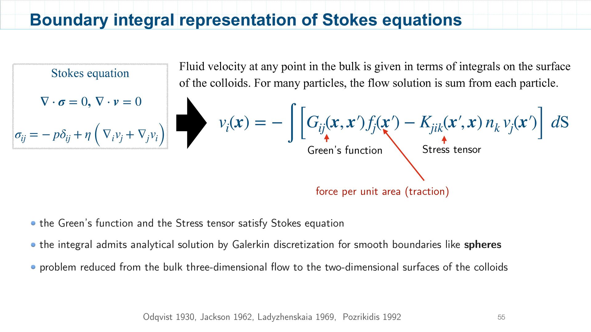
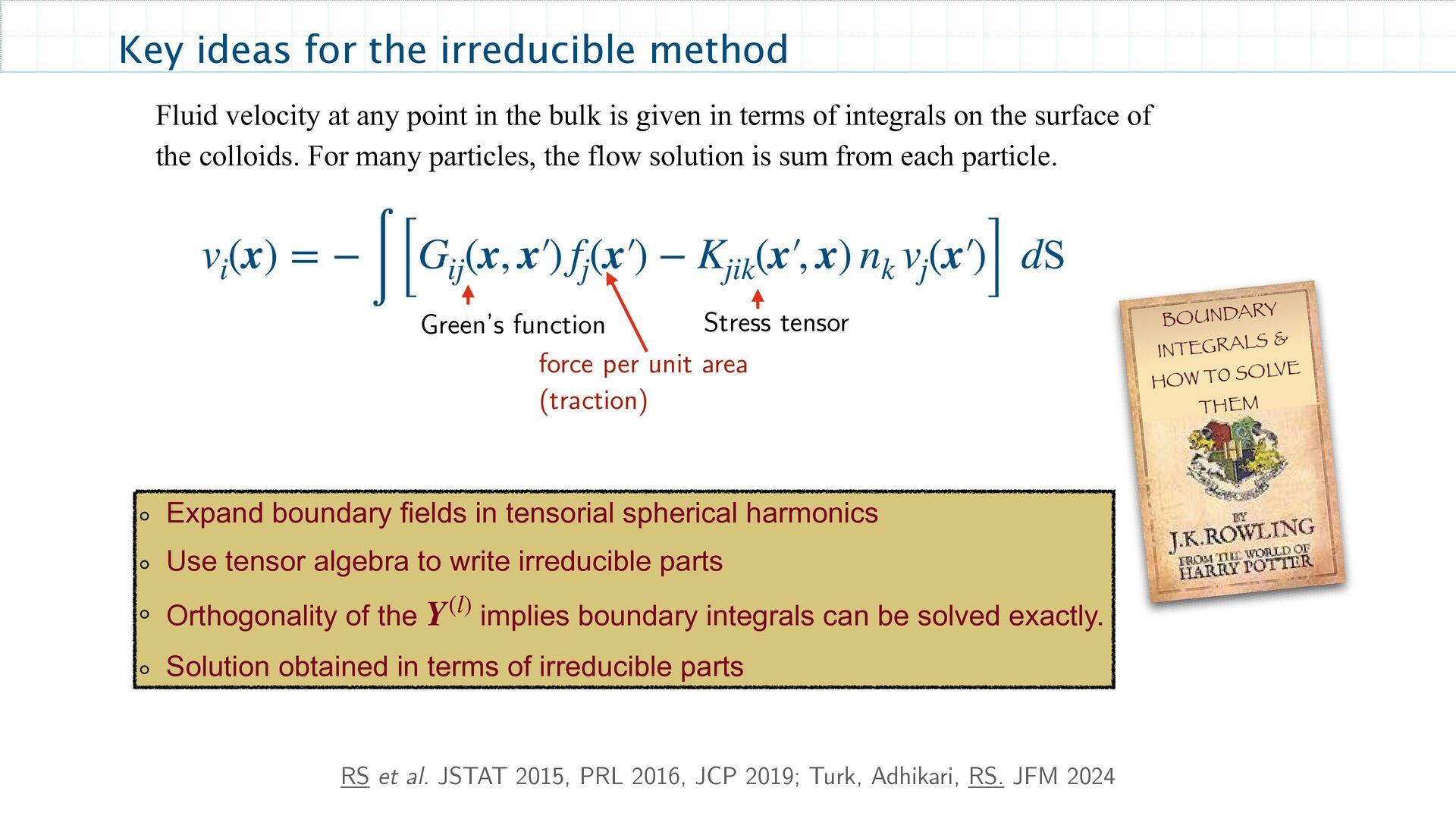
in terms of integrals on the surface of the colloids. For many particles, the flow solution is sum from each particle. Green’s function Stress tensor the Green’s function and the Stress tensor satisfy Stokes equation the integral admits analytical solution by Galerkin discretization for smooth boundaries like spheres problem reduced from the bulk three-dimensional flow to the two-dimensional surfaces of the colloids Odqvist 1930, Jackson 1962, Ladyzhenskaia 1969, Pozrikidis 1992 55 force per unit area (traction) Boundary integral representation of Stokes equations Stokes equation , ∇ ⋅ σ = 0 ∇ ⋅ v = 0 σ ij = − pδ ij + η ( ∇ i v j + ∇ j v i) v i (x) = − ∫ [ G ij (x, x′ ) f j (x′ ) − K jik (x′ , x) n k v j (x′ ) ] dS
2015, PRL 2016, JCP 2019; Turk, Adhikari, RS. JFM 2024 Expand boundary fields in tensorial spherical harmonics Use tensor algebra to write irreducible parts Orthogonality of the implies boundary integrals can be solved exactly. Solution obtained in terms of irreducible parts Y(l) BOUNDARY INTEGRALS & HOW T0 SOLVE THEM Fluid velocity at any point in the bulk is given in terms of integrals on the surface of the colloids. For many particles, the flow solution is sum from each particle. Green’s function Stress tensor force per unit area (traction) v i (x) = − ∫ [ G ij (x, x′ ) f j (x′ ) − K jik (x′ , x) n k v j (x′ ) ] dS
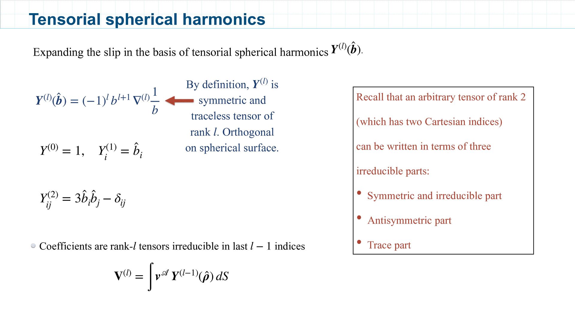
b i Y(l)( ̂ b) = (−1)l bl+1 ∇(l) 1 b By definition, is symmetric and traceless tensor of rank . Orthogonal on spherical surface. Y(l) l Recall that an arbitrary tensor of rank 2 (which has two Cartesian indices) can be written in terms of three irreducible parts: • Symmetric and irreducible part • Antisymmetric part • Trace part Coefficients are rank- tensors irreducible in last indices l l − 1 V(l) = ∫ v Y(l−1)( ̂ ρ) dS Y(2) ij = 3 ̂ b i ̂ b j − δ ij Expanding the slip in the basis of tensorial spherical harmonics . Y(l)( ̂ b)
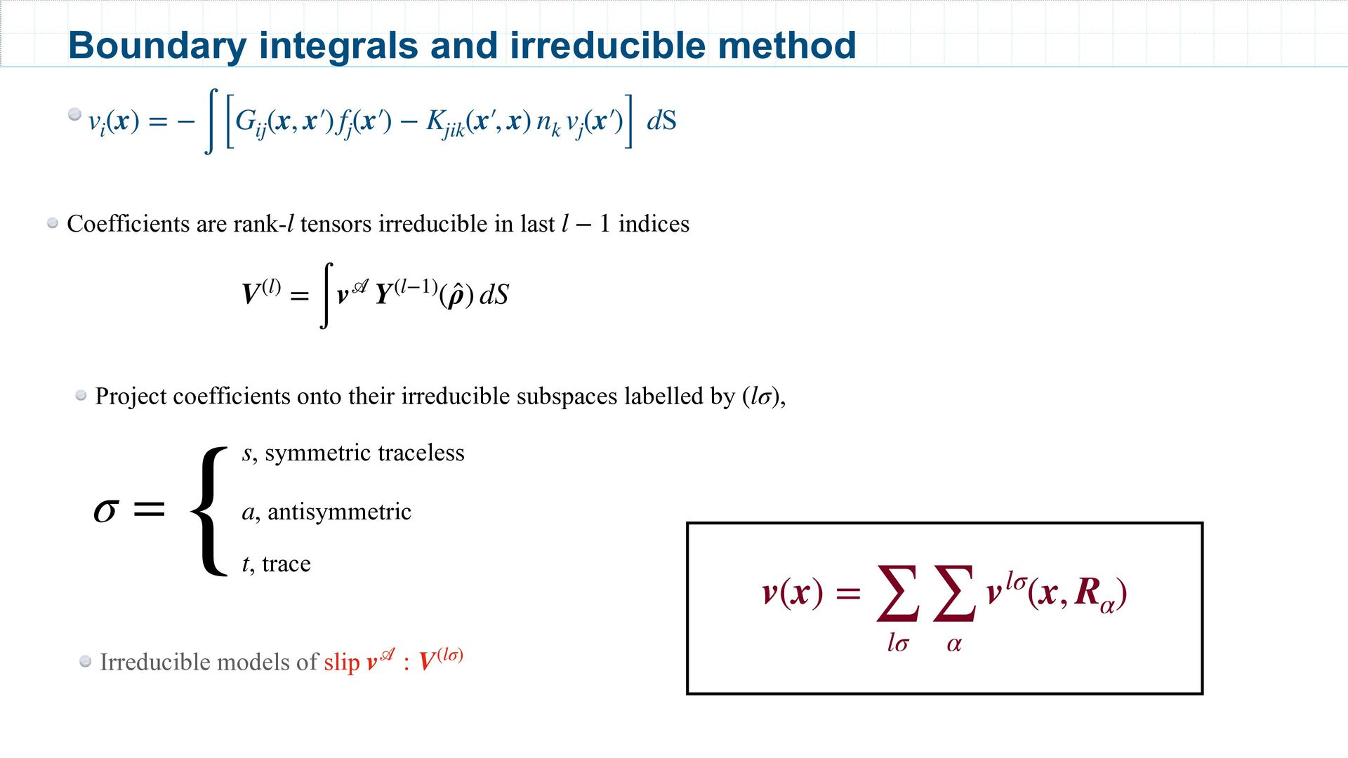
− 1 V(l) = ∫ v Y(l−1)( ̂ ρ) dS Project coefficients onto their irreducible subspaces labelled by , (lσ) σ = { , symmetric traceless s , antisymmetric a , trace t Boundary integrals and irreducible method Irreducible models of slip v : V(lσ) v i (x) = − ∫ [ G ij (x, x′ ) f j (x′ ) − K jik (x′ , x) n k v j (x′ ) ] dS v(x) = ∑ lσ ∑ α vlσ(x, Rα )
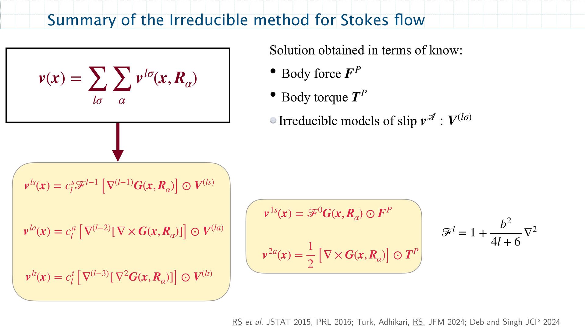
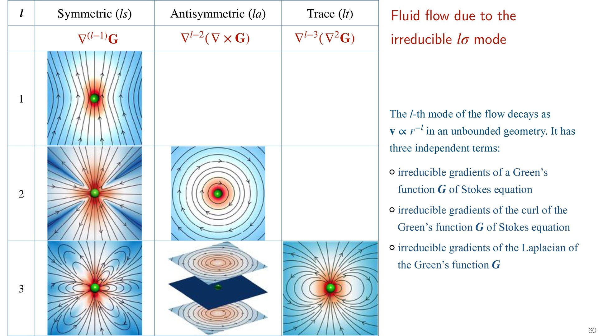
∇l−2(∇ × G) ∇(l−1)G ∇l−3(∇2G) Fluid flow due to the irreducible mode lσ 60 The l-th mode of the flow decays as in an unbounded geometry. It has three independent terms: irreducible gradients of a Green’s function of Stokes equation irreducible gradients of the curl of the Green’s function of Stokes equation irreducible gradients of the Laplacian of the Green’s function v ∝ r−l G G G
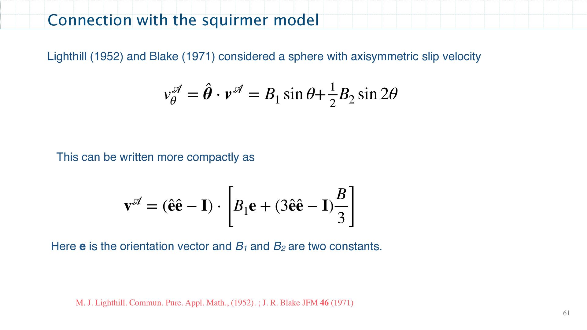
axisymmetric slip velocity Connection with the squirmer model This can be written more compactly as Here e is the orientation vector and B1 and B2 are two constants. v = ( ̂ e ̂ e − I) ⋅ [ B 1 e + (3 ̂ e ̂ e − I) B 3 ] v θ = ̂ θ ⋅ v = B 1 sin θ+ 1 2 B 2 sin 2θ M. J. Lighthill. Commun. Pure. Appl. Math., (1952). ; J. R. Blake JFM 46 (1971)
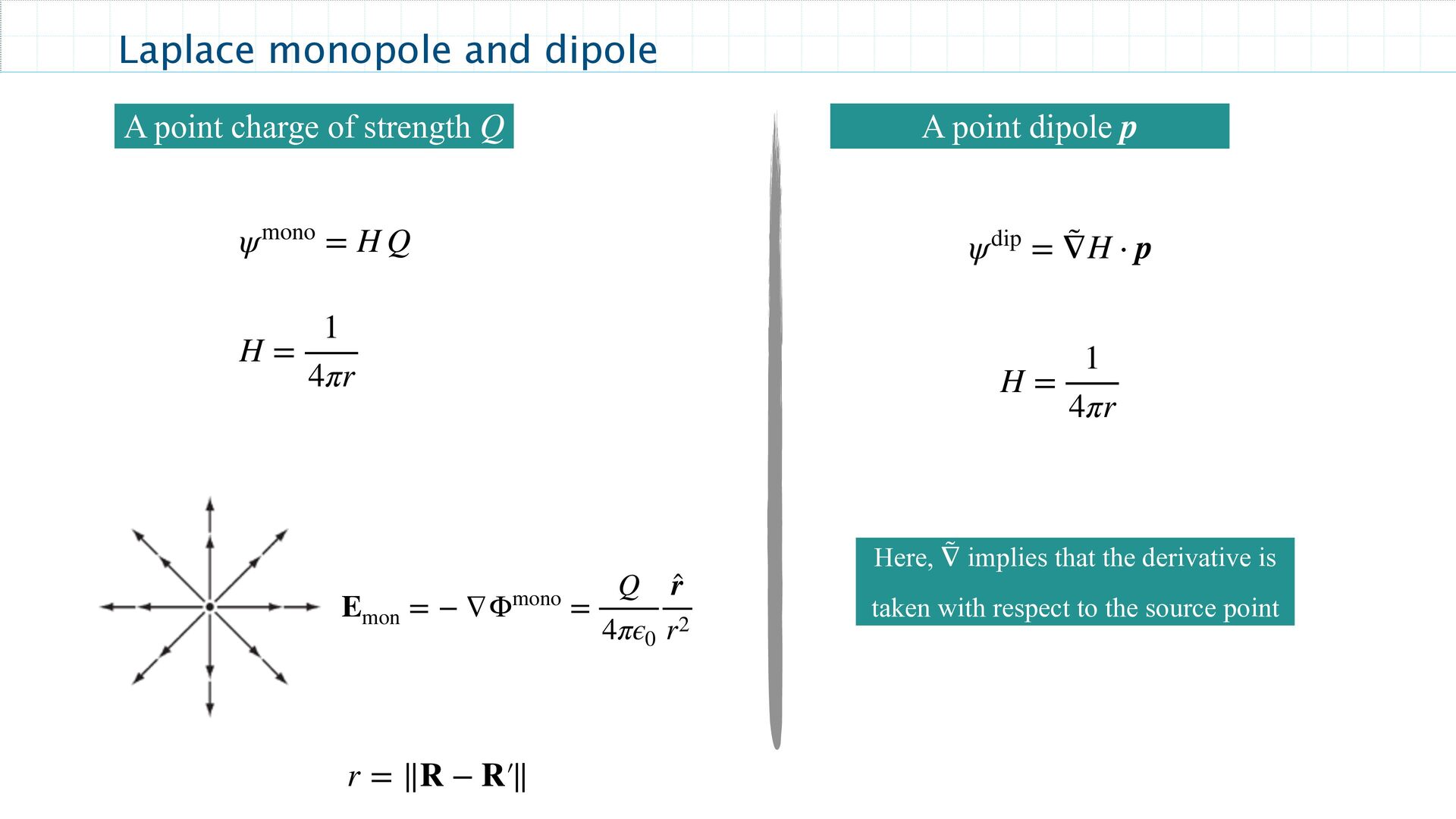
˜ ∇H ⋅ p H = 1 4πr Here, implies that the derivative is taken with respect to the source point ˜ ∇ H = 1 4πr ψmono = H Q A point charge of strength Q E mon = − ∇Φmono = Q 4πϵ0 ̂ r r2 r = ∥R − R′ ∥
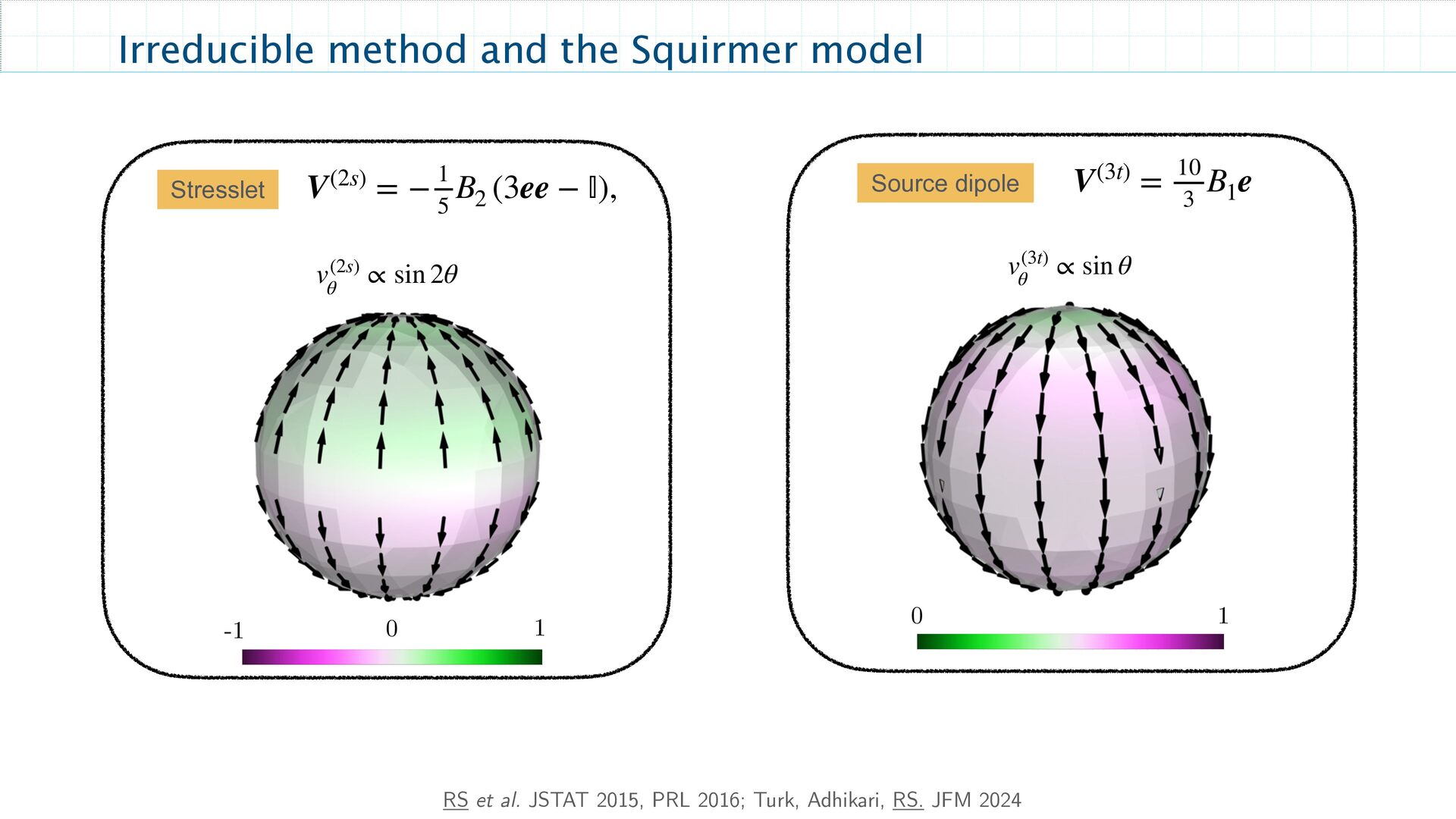
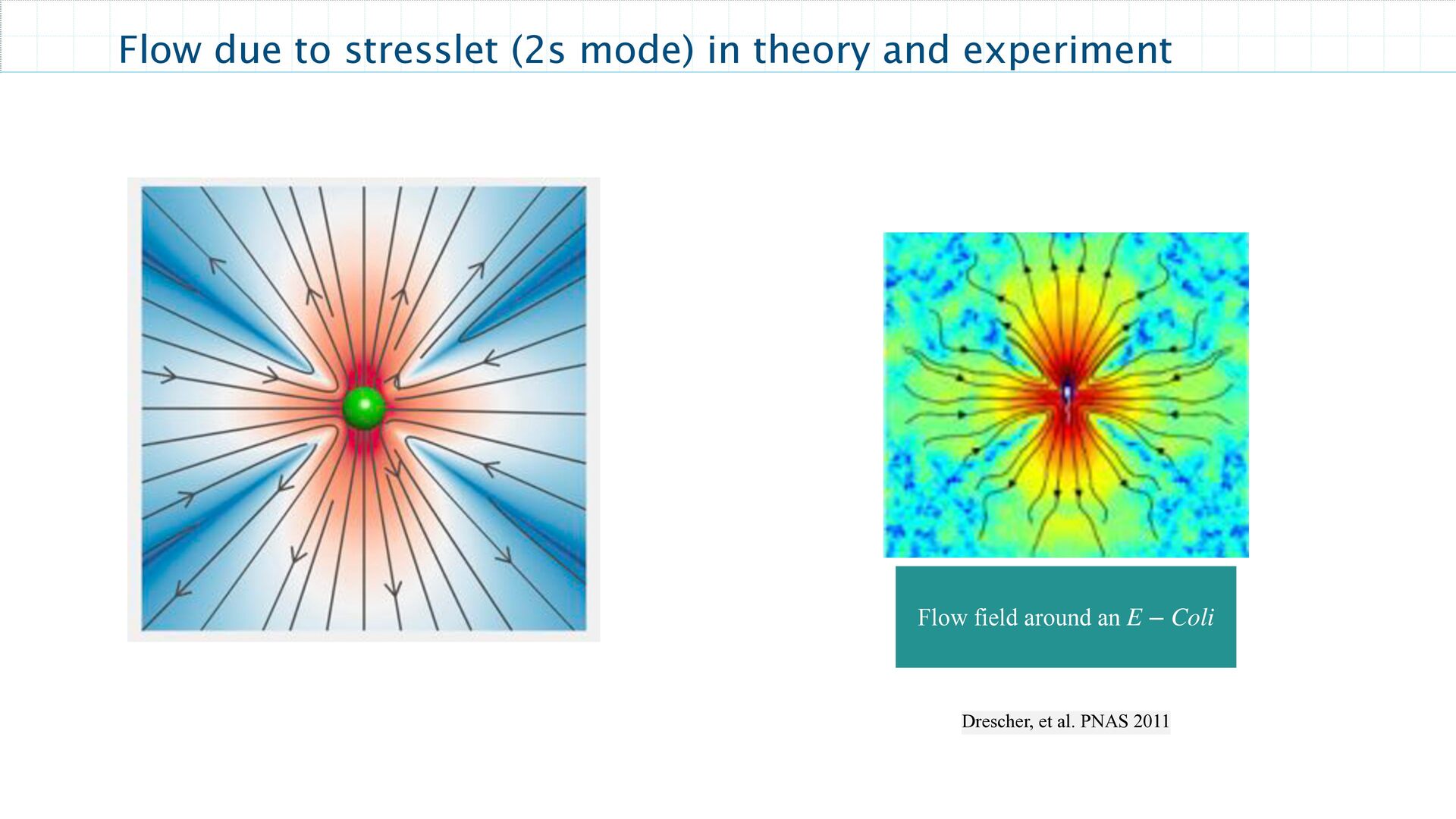
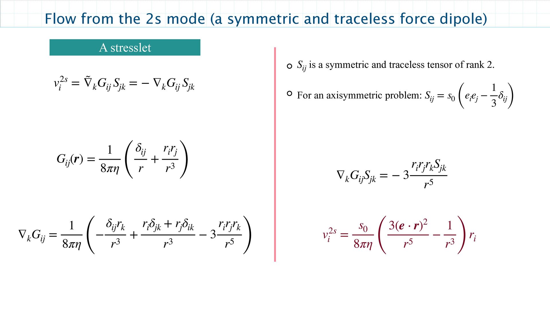
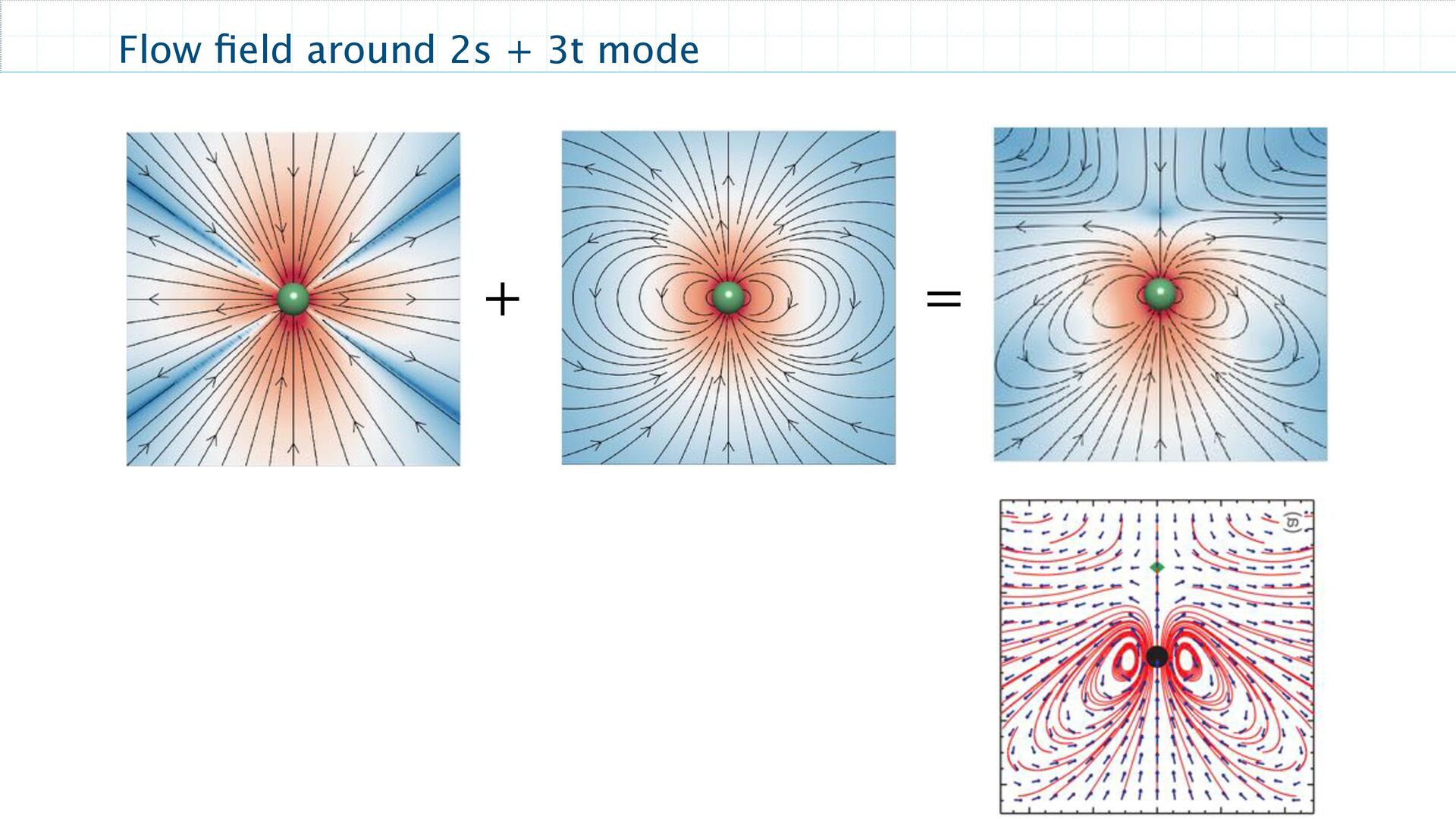
dipole) v2s i = ˜ ∇ k G ij S jk = − ∇ k G ij S jk G ij (r) = 1 8πη ( δ ij r + r i r j r3 ) A stresslet is a symmetric and traceless tensor of rank 2. For an axisymmetric problem: S ij S ij = s 0 ( e i e j − 1 3 δ ij) ∇ k G ij = 1 8πη ( − δ ij r k r3 + r i δ jk + r j δ ik r3 − 3 r i r j r k r5 ) ∇ k G ij S jk = − 3 r i r j r k S jk r5 v2s i = s 0 8πη ( 3(e ⋅ r)2 r5 − 1 r3 ) r i
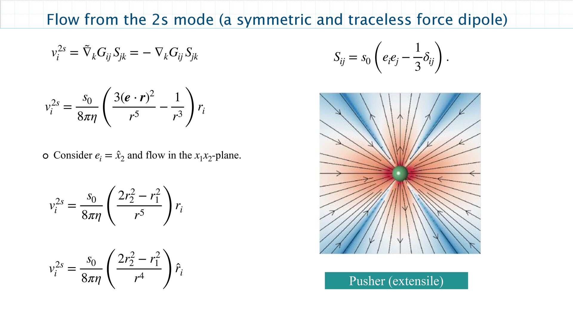
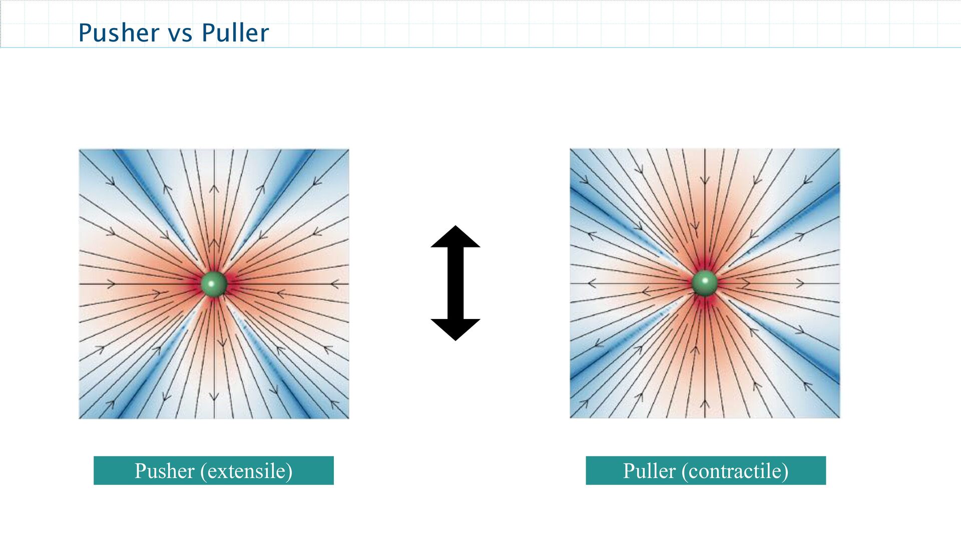
dipole) Consider and flow in the -plane. e i = ̂ x 2 x 1 x 2 v2s i = s 0 8πη ( 2r2 2 − r2 1 r5 ) r i v2s i = s 0 8πη ( 2r2 2 − r2 1 r4 ) ̂ r i v2s i = s 0 8πη ( 3(e ⋅ r)2 r5 − 1 r3 ) r i v2s i = ˜ ∇ k G ij S jk = − ∇ k G ij S jk Pusher (extensile) S ij = s 0 ( e i e j − 1 3 δ ij) .
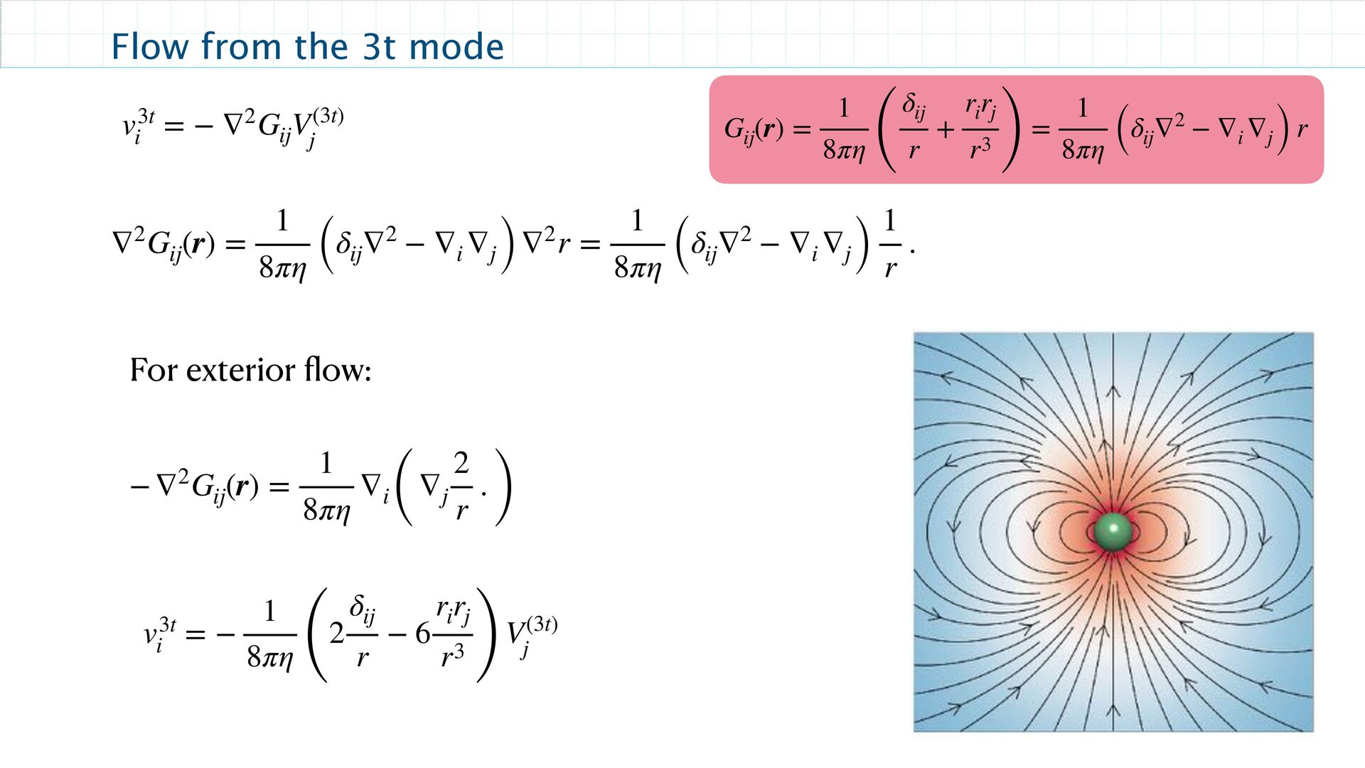
ij V(3t) j ∇2G ij (r) = 1 8πη ( δ ij ∇2 − ∇ i ∇ j) ∇2r = 1 8πη ( δ ij ∇2 − ∇ i ∇ j) 1 r . −∇2G ij (r) = 1 8πη ∇ i( ∇ j 2 r . ) For exterior ow: v3t i = − 1 8πη ( 2 δ ij r − 6 r i r j r3 ) V(3t) j G ij (r) = 1 8πη ( δ ij r + r i r j r3 ) = 1 8πη ( δ ij ∇2 − ∇ i ∇ j) r
= μT 0 FP α + VHI α , VHI α = N ∑ i≠j μTT αβ ⊙ FP β F α = − ∇ α U The net potential is a sum of: • spring potential for connecting the beads by spring and • bending potential which makes the chain rigid U Uspring Ubend r 0 Uspring = 1 2 κ s (r − r 0) 2 Ubend = κ s (1 − cos ϕ) ADD ONE ACTIVE BEAD
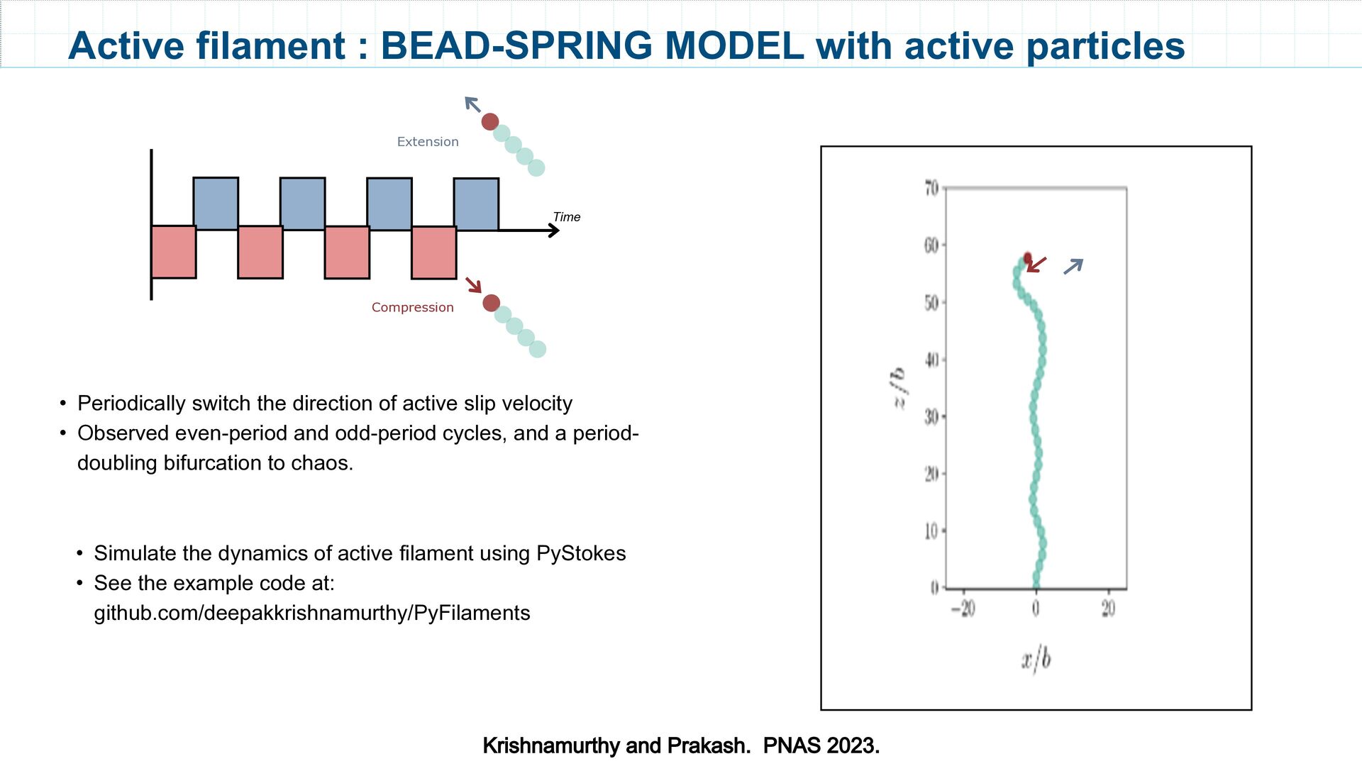
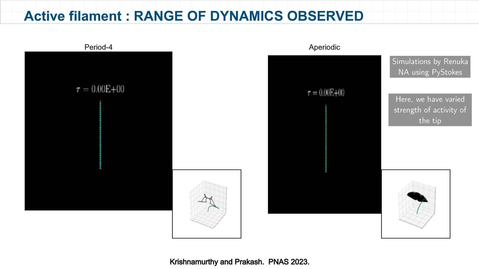
Compression • Periodically switch the direction of active slip velocity • Observed even-period and odd-period cycles, and a period- doubling bifurcation to chaos. • Simulate the dynamics of active filament using PyStokes • See the example code at: github.com/deepakkrishnamurthy/PyFilaments Krishnamurthy and Prakash. PNAS 2023.
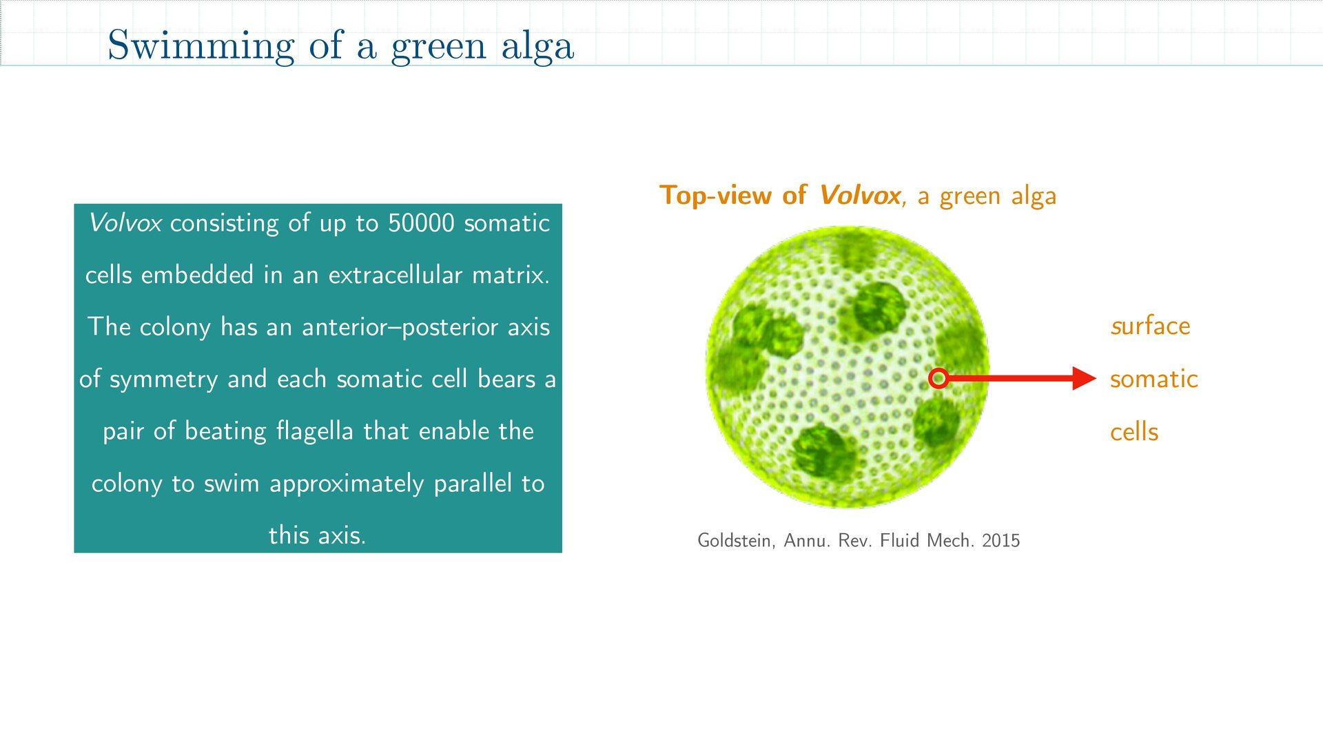
Mech. 2015 surface somatic cells Top-view of Volvox, a green alga Volvox consisting of up to 50000 somatic cells embedded in an extracellular matrix. The colony has an anterior–posterior axis of symmetry and each somatic cell bears a pair of beating flagella that enable the colony to swim approximately parallel to this axis.
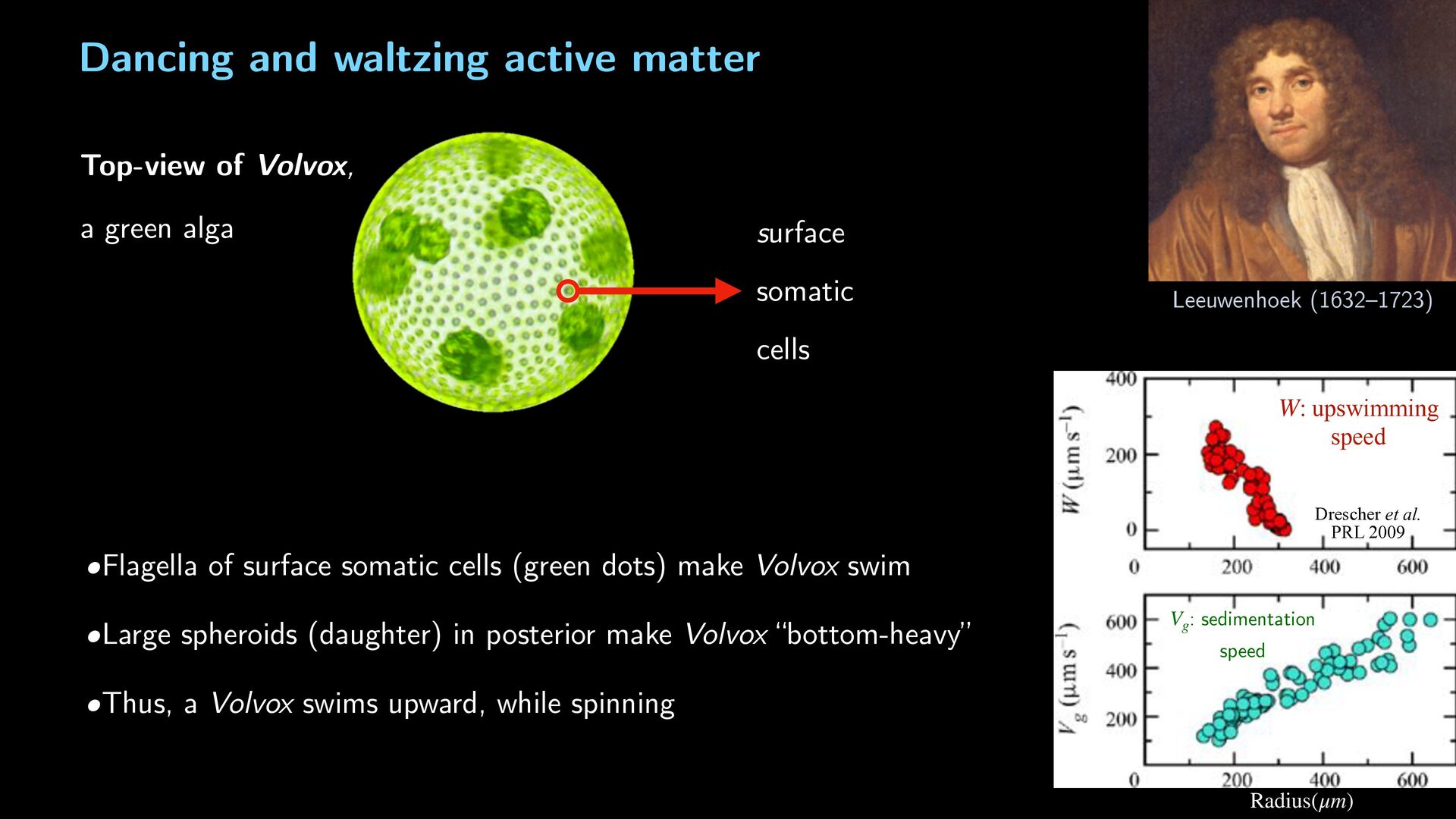
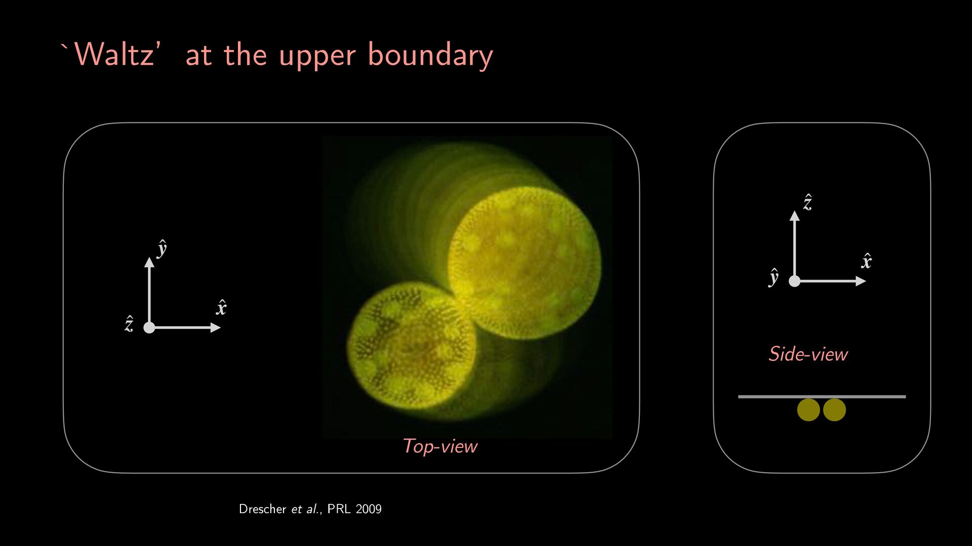
•Large spheroids (daughter) in posterior make Volvox “bottom-heavy” •Thus, a Volvox swims upward, while spinning Top-view of Volvox, a green alga surface somatic cells Dancing and waltzing active matter Leeuwenhoek (1632–1723) U = W + V g : upswimming speed W : sedimentation speed V g Radius(μm) Drescher et al. PRL 2009
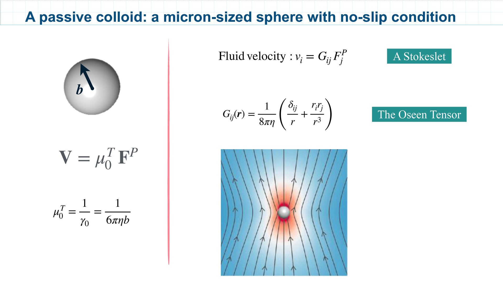
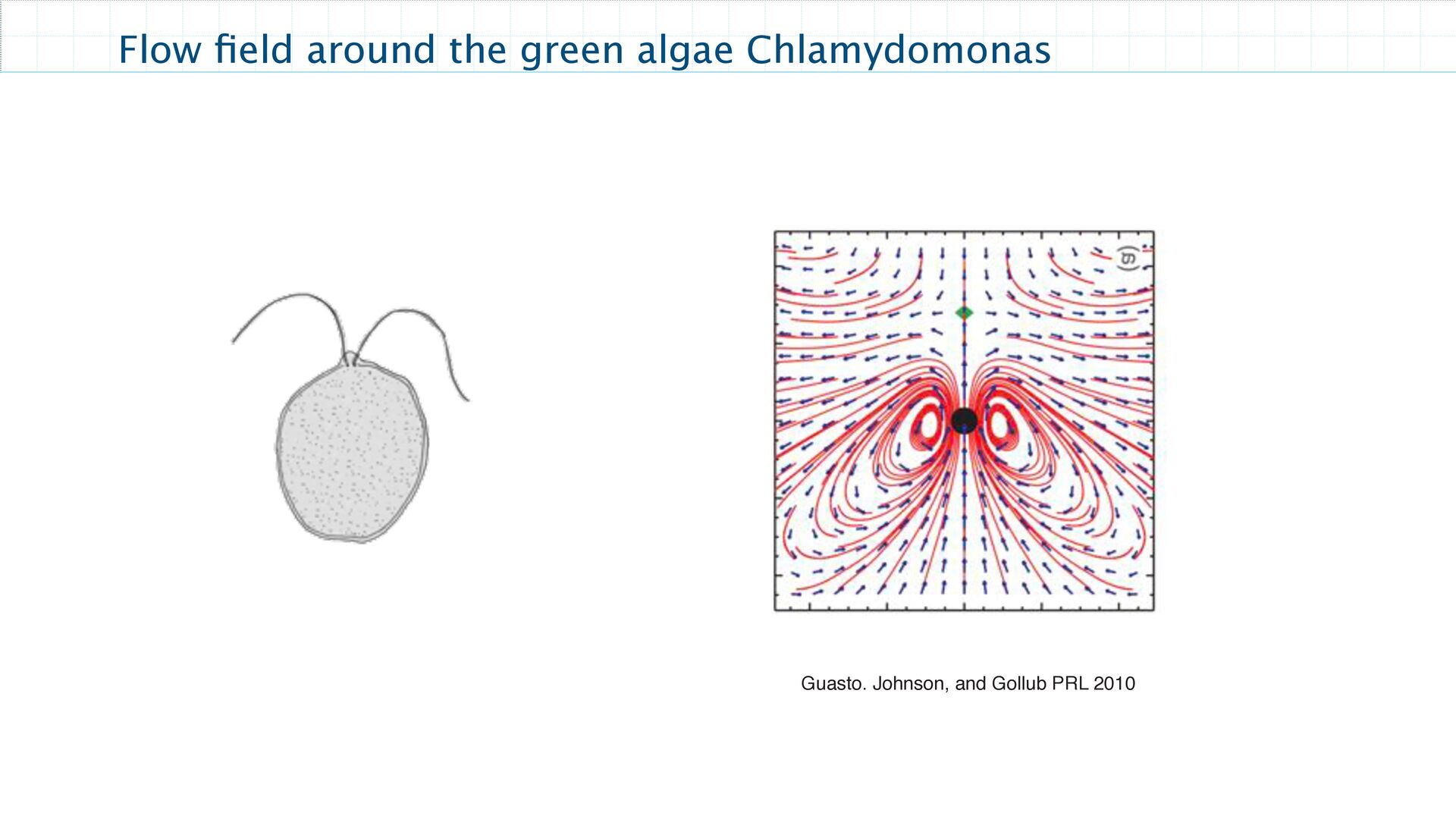
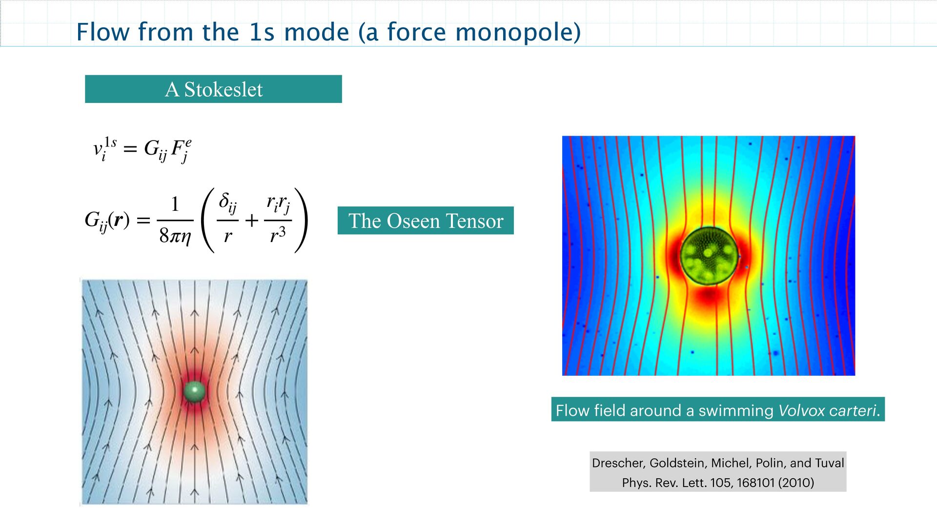
around a swimming Volvox carteri. Drescher, Goldstein, Michel, Polin, and Tuval Phys. Rev. Lett. 105, 168101 (2010) v1s i = G ij Fe j G ij (r) = 1 8πη ( δ ij r + r i r j r3 ) A Stokeslet The Oseen Tensor
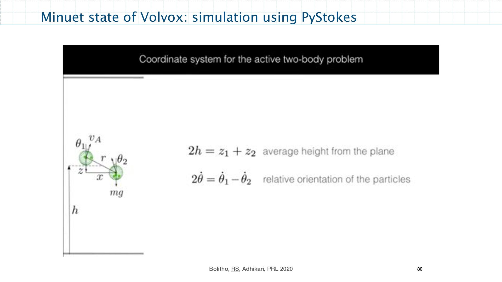
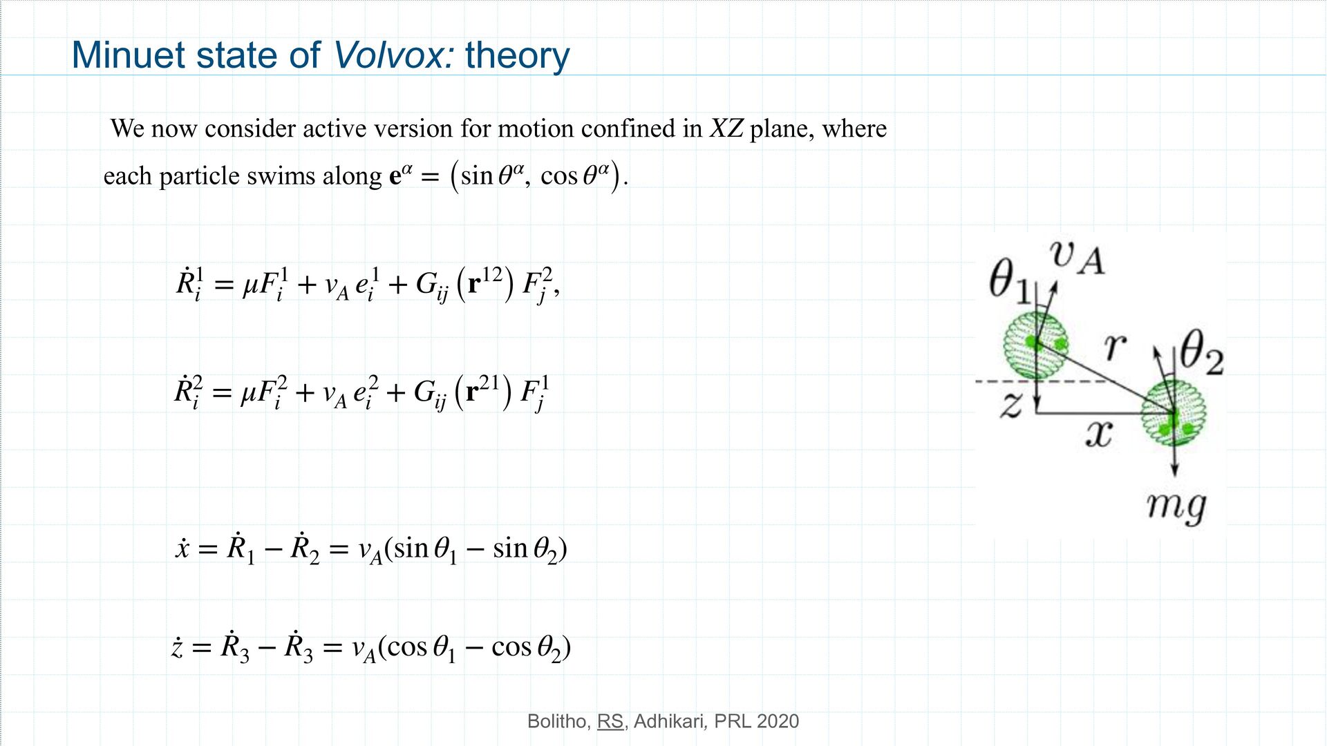
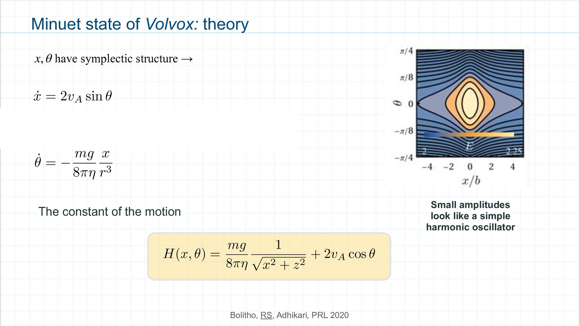
We now consider active version for motion confined in plane, where each particle swims along . XZ eα = (sin θα, cos θα ) · R1 i = μF1 i + v A e1 i + G ij (r12 ) F2 j , · R2 i = μF2 i + v A e2 i + G ij (r21 ) F1 j · x = · R 1 − · R 2 = v A (sin θ 1 − sin θ 2 ) · z = · R 3 − · R 3 = v A (cos θ 1 − cos θ 2 )
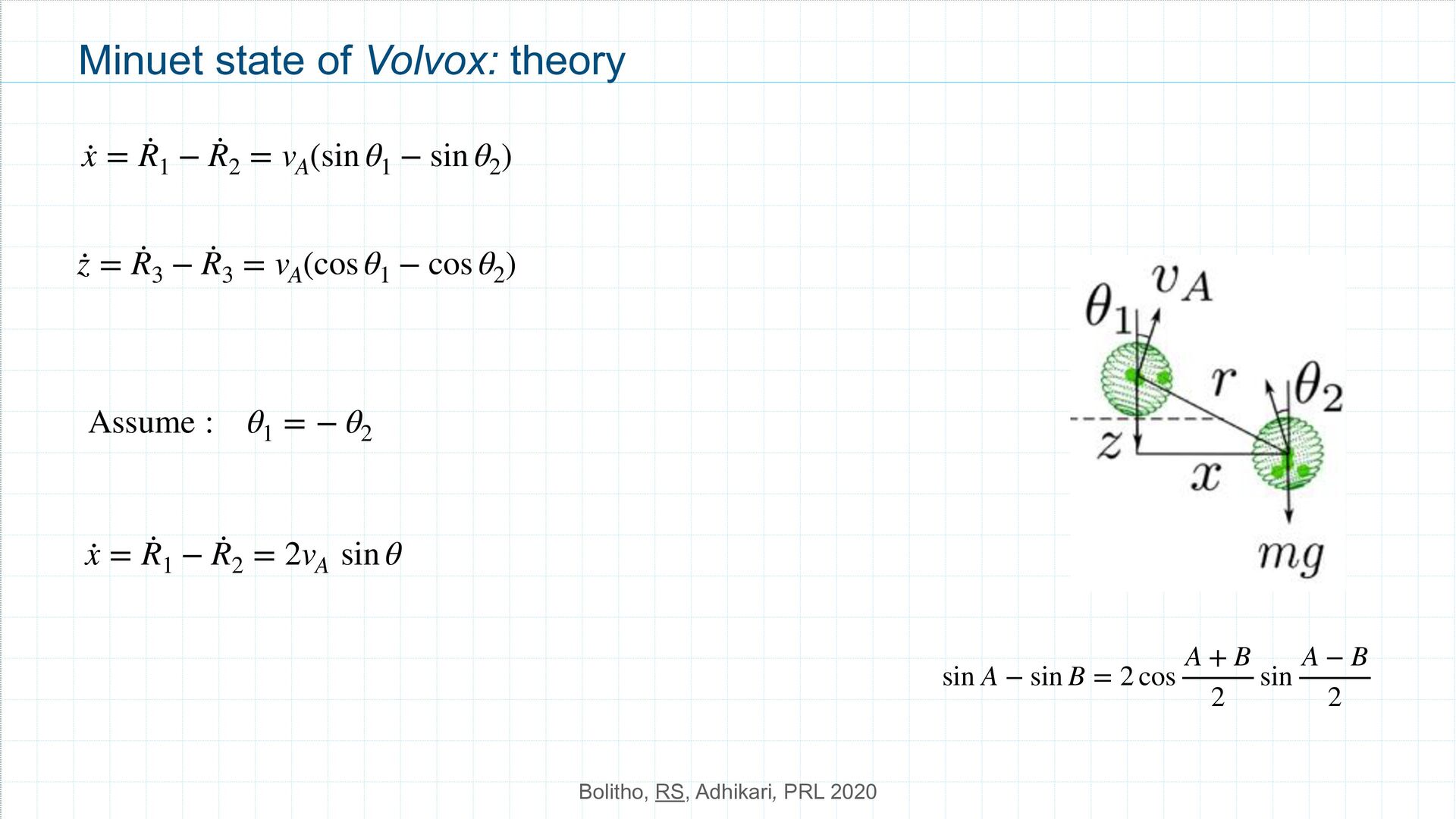
· x = · R 1 − · R 2 = v A (sin θ 1 − sin θ 2 ) · z = · R 3 − · R 3 = v A (cos θ 1 − cos θ 2 ) sin A − sin B = 2 cos A + B 2 sin A − B 2 Assume : θ 1 = − θ 2 · x = · R 1 − · R 2 = 2v A sin θ
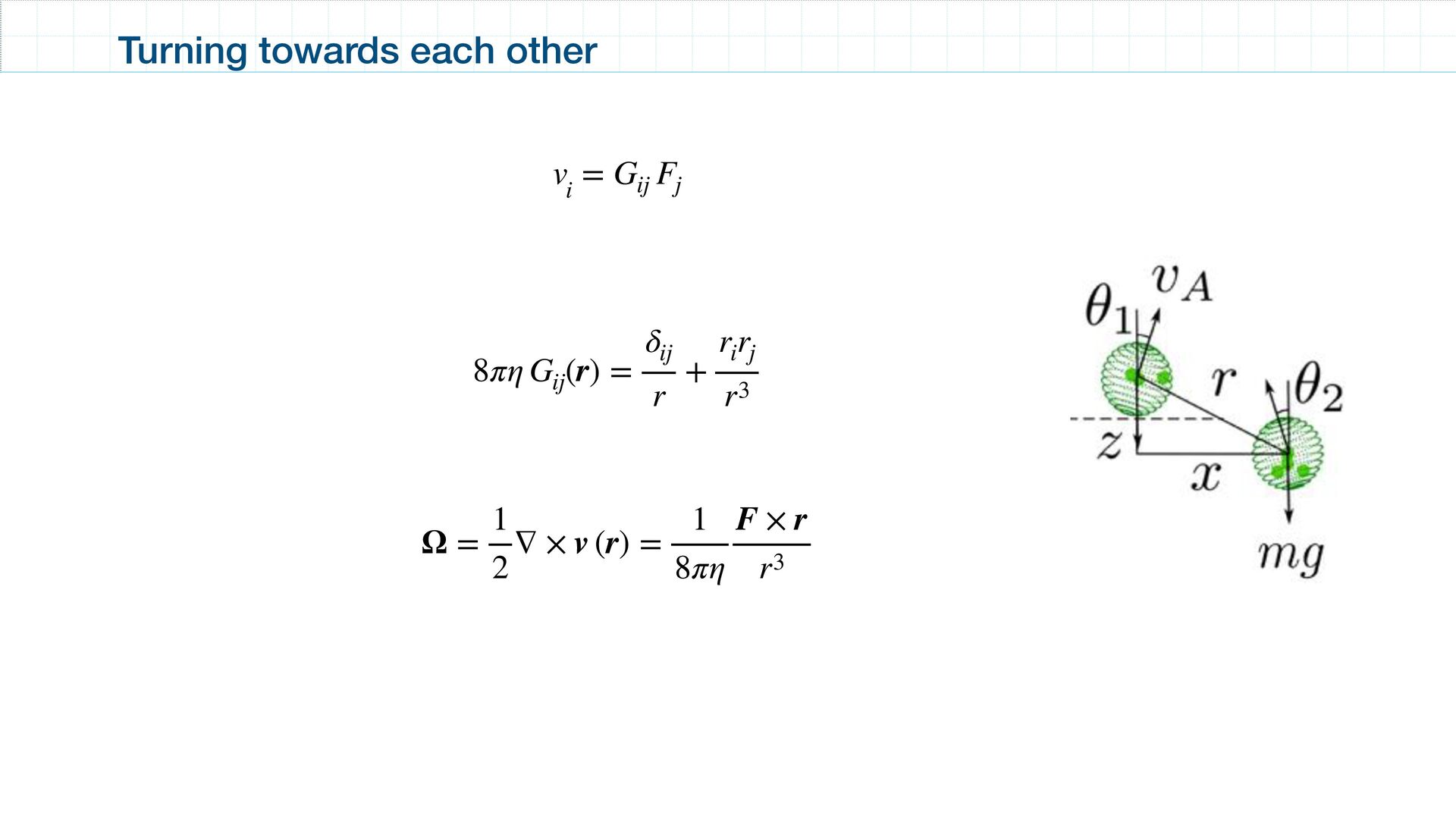
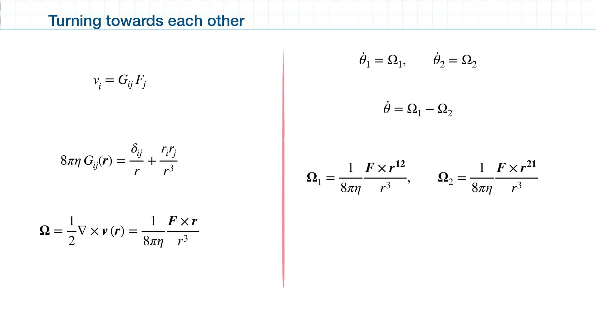
v (r) = 1 8πη F × r r3 v i = G ij F j 8πη G ij (r) = δ ij r + r i r j r3 · θ 1 = Ω 1 , · θ 2 = Ω 2 · θ = Ω 1 − Ω 2 Ω 1 = 1 8πη F × r12 r3 , Ω 2 = 1 8πη F × r21 r3
<latexit sha1_base64="U765SeWuvaKMdC1/ZCCMyWHMGMQ=">AAACpXicbVFdT9swFHUytkH3VcYjLxHVNqZpVVIqxgsSjBdekGCiBakukeM6jYXjRPYNorP8z/Yr9sa/mZsEiQFXsnzuOffDvjcpBdcQhnee/2Ll5avXq2udN2/fvf/QXf841kWlKBvRQhTqMiGaCS7ZCDgIdlkqRvJEsIvk+mipX9wwpXkhz2FRsmlO5pKnnBJwVNz9g2cFmFv7eX9wE5tDizWXGDIGBONaypzUKLTQuNS8vuuI7zhVhJp8bs0eLjl2lMWCpbDdCENrdhL7rXEia9Q9/n1lBtb5V2bHWqz4PIOvbbumsuv5bPGaur3P7MTdXtgPawuegqgFPdTaadz965rQKmcSqCBaT6KwhKkhCjgVzHZwpVlJ6DWZs4mDkuRMT009ZRt8cswsSAvljoSgZh9mGJJrvcgTF5kTyPRjbUk+p00qSPemhsuyAiZp0yitRABFsFxZMOOKURALBwhV3L01oBlxowC32OUQosdffgrGg3602x+eDXsHP9txrKJNtIW2UYR+oAN0jE7RCFFvyzv2zrxf/hf/xD/3x02o77U5G+g/8+N/L3fVGQ==</latexit> ˙ x = 2vA sin ✓ ˙ h = vA cos cos ✓ mg 8⇡⌘ ✓ 4 3b + 1 r + z2 r3 ◆ ˙ ✓ = mg 8⇡⌘ x r3 have symplectic structure → x, θ The constant of the motion <latexit sha1_base64="FwQLrpbRgLZow0cM5aoc6F7aXeQ=">AAACNnicbVDLSgMxFM34rPVVdelmsAiKUmaKohvBx8aNUMFWoVNLJs20wczD5E6xhnyVG7/DnRsXirj1E8y0XWjrgYTDOffe5B4/4UyC47xaE5NT0zOzubn8/MLi0nJhZbUm41QQWiUxj8WNjyXlLKJVYMDpTSIoDn1Or/27s8y/7lIhWRxdQS+hjRC3IxYwgsFIzcLF+dbDrgcdCnj7yAsEJipsa3XoJcwzmh5IrlaevBegHm5VWe88ZrfWO+VuU51oj8RyMCHfLBSdktOHPU7cISmiISrNwovXikka0ggIx1LWXSeBhsICGOFU571U0gSTO9ymdUMjHFLZUP21tb1plJYdxMKcCOy++rtD4VDKXuibyhBDR456mfifV08hOGwoFiUp0IgMHgpSbkNsZxnaLSYoAd4zBBPBzF9t0sEmKDBJZyG4oyuPk1q55O6XnMu94vHpMI4cWkcbaAu56AAdo3NUQVVE0BN6Re/ow3q23qxP62tQOmENe9bQH1jfP/IyrUg=</latexit> H(x, ✓) = mg 8⇡⌘ 1 p x2 + z2 + 2vA cos ✓ Small amplitudes look like a simple harmonic oscillator
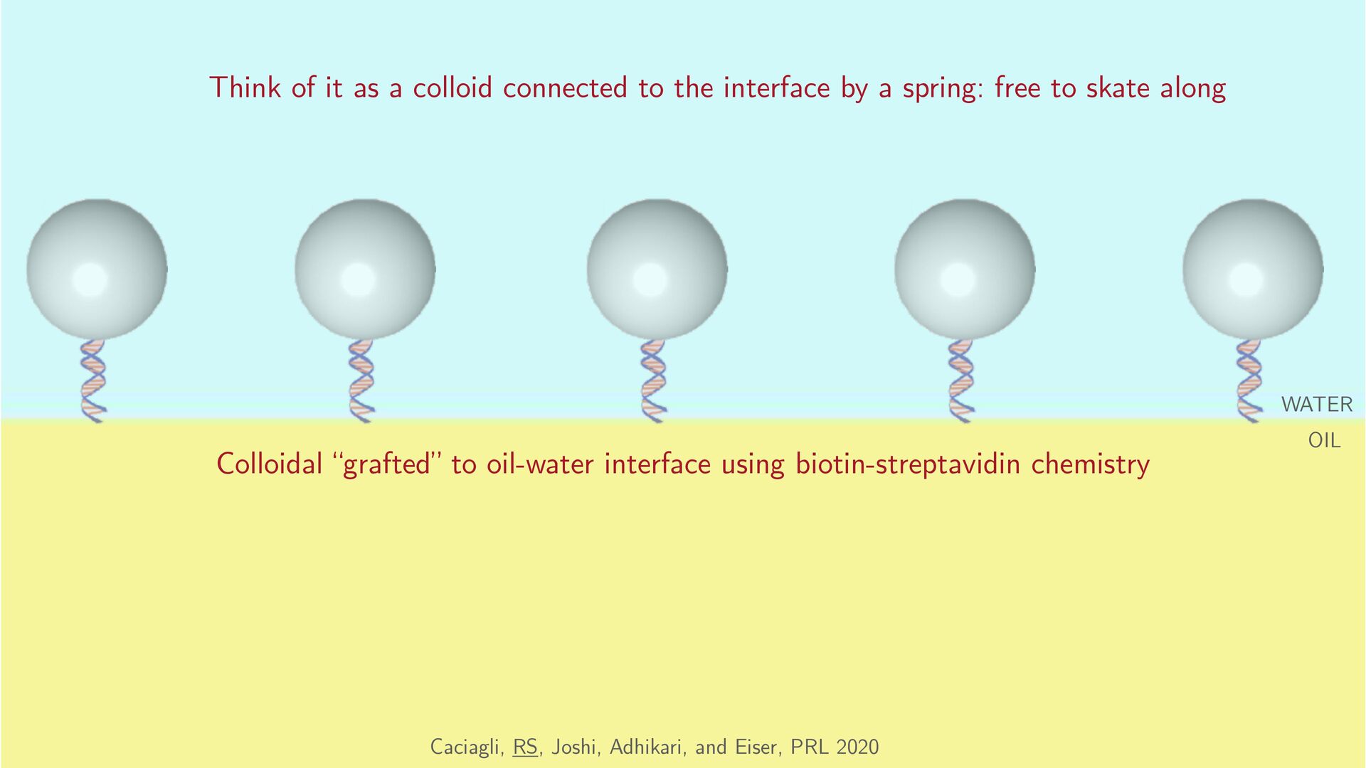
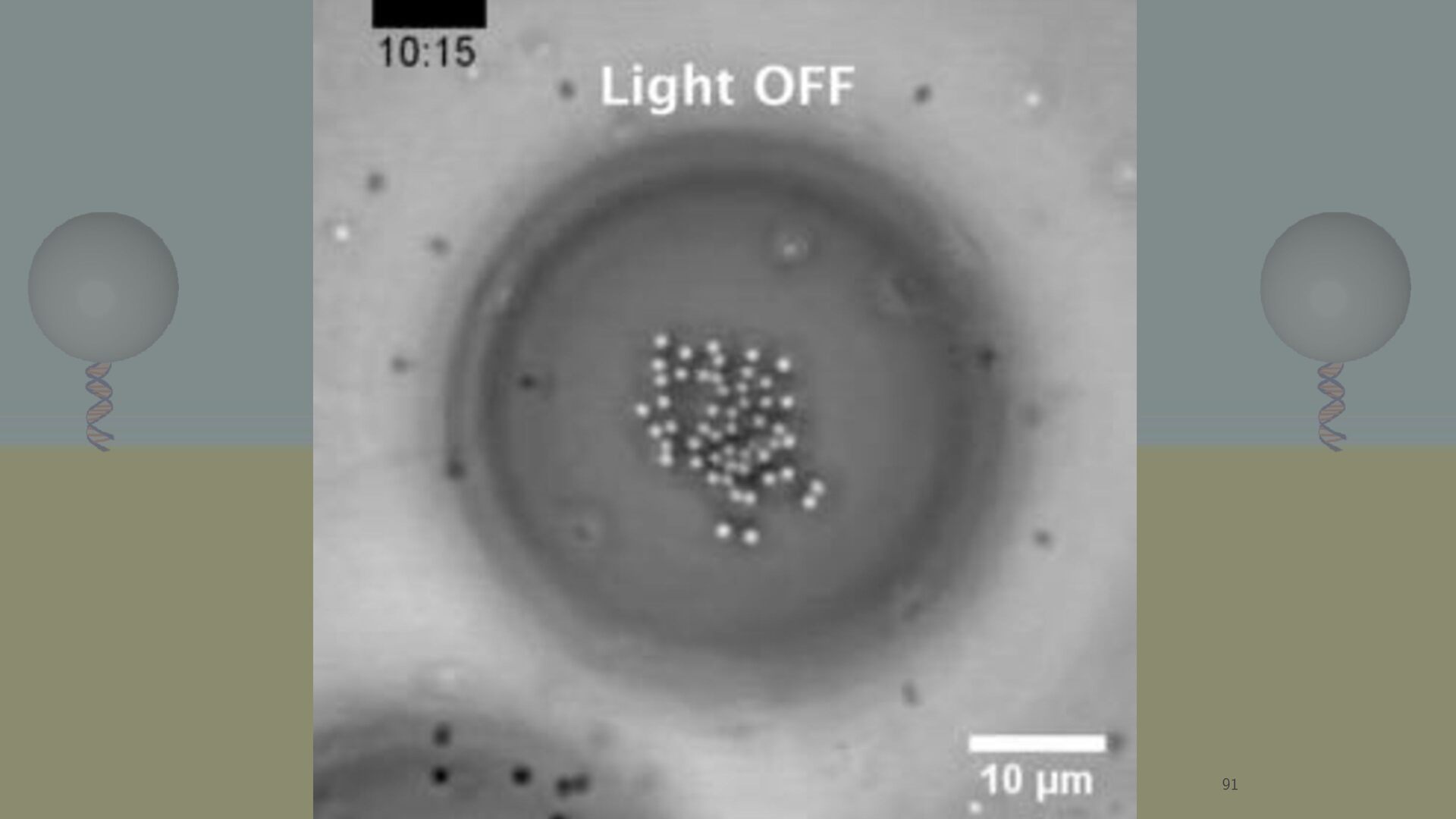
to oil-water interface using biotin-streptavidin chemistry Think of it as a colloid connected to the interface by a spring: free to skate along OIL WATER
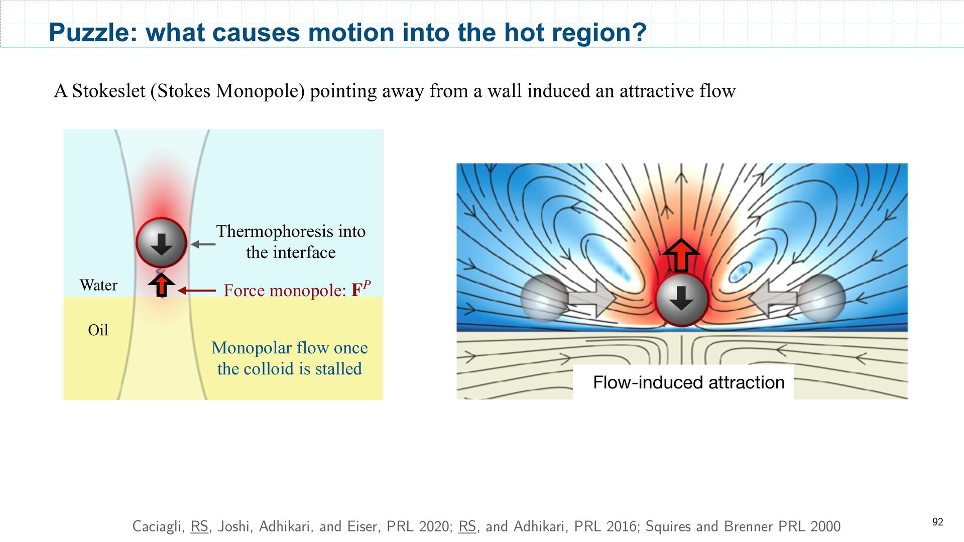
and Adhikari, PRL 2016; Squires and Brenner PRL 2000 Water Oil Monopolar flow once the colloid is stalled Thermophoresis into the interface Flow-induced attraction Puzzle: what causes motion into the hot region? A Stokeslet (Stokes Monopole) pointing away from a wall induced an attractive flow Force monopole: FP
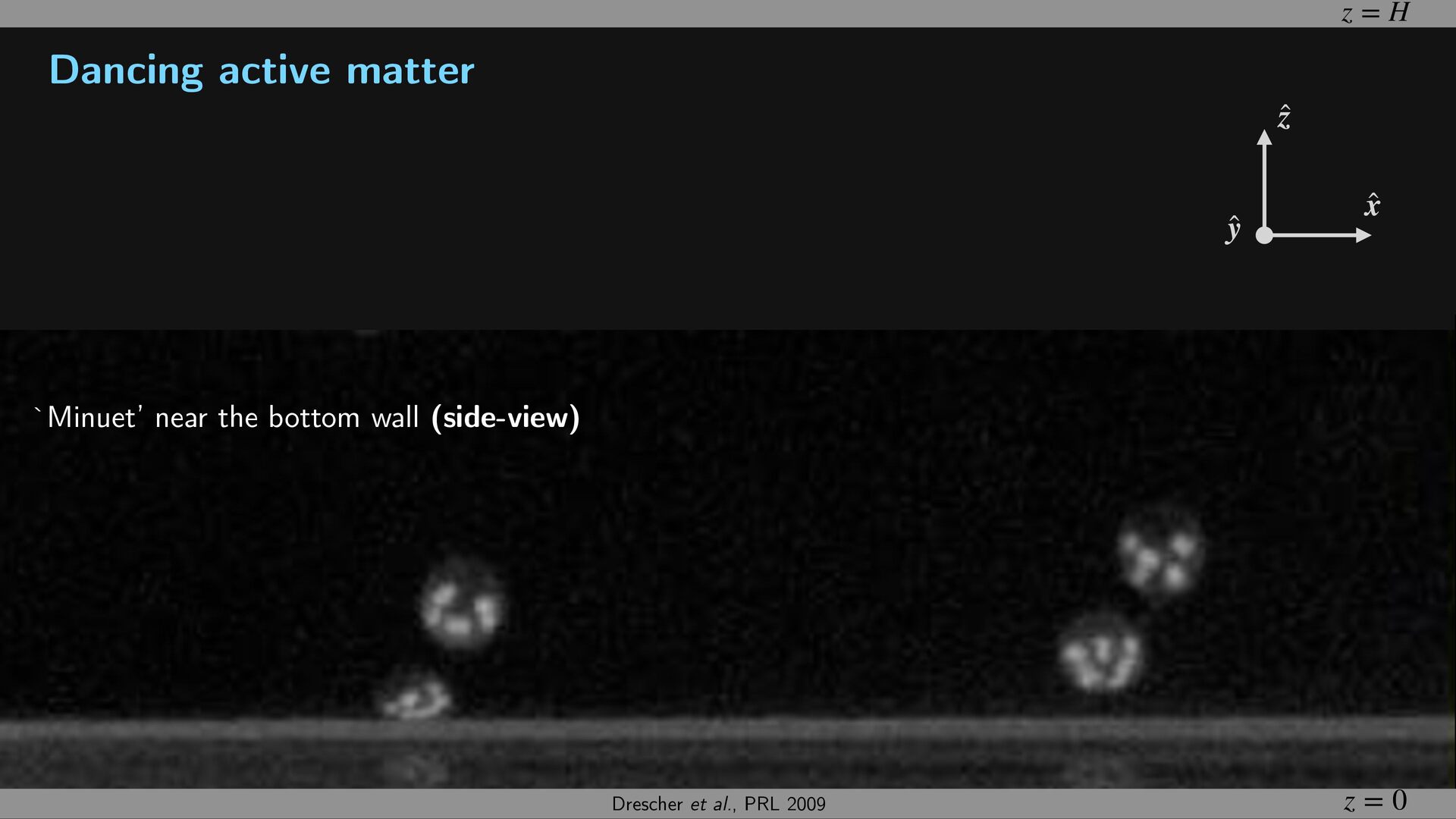
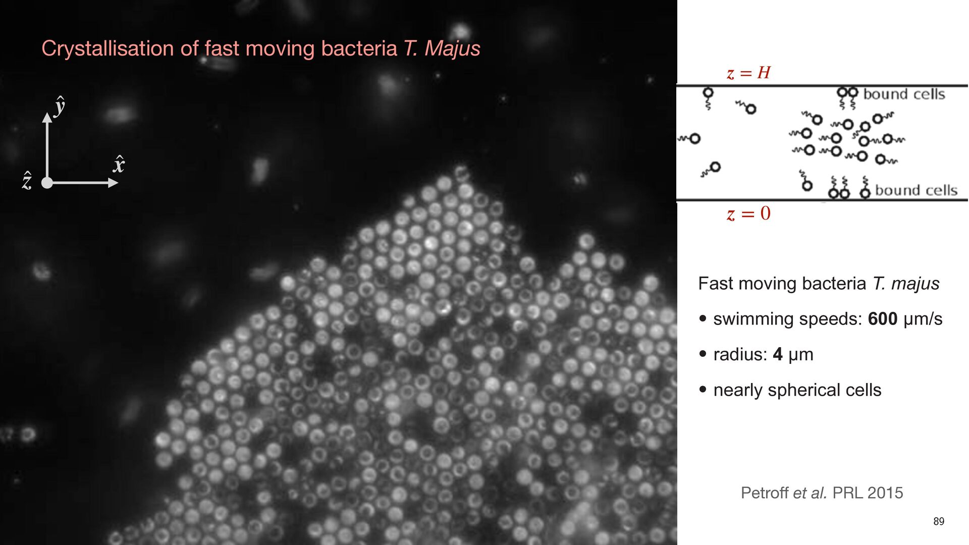
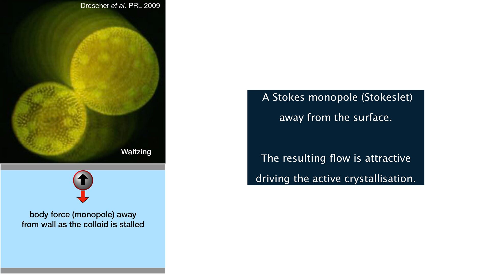
stalled Waltzing Drescher et al. PRL 2009 A Stokes monopole (Stokeslet) away from the surface. The resulting flow is attractive driving the active crystallisation.
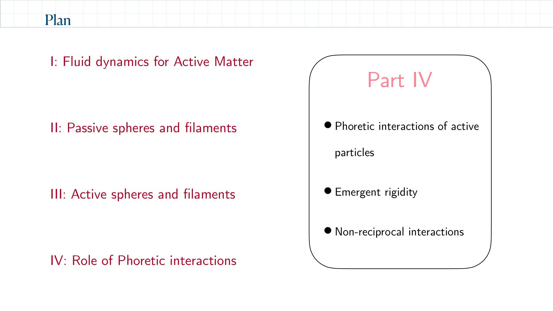
rigidity • Non-reciprocal interactions Part IV I: Fluid dynamics for Active Matter II: Passive spheres and filaments IV: Role of Phoretic interactions III: Active spheres and filaments
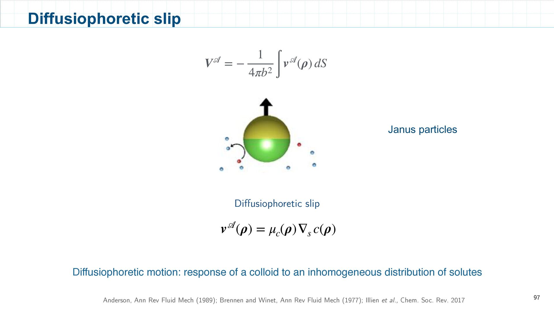
Rev Fluid Mech (1977); Illien et al., Chem. Soc. Rev. 2017 v (ρ) = μ c (ρ)∇ s c(ρ) Diffusiophoretic slip Diffusiophoretic motion: response of a colloid to an inhomogeneous distribution of solutes 97 Diffusiophoretic slip V = − 1 4πb2 ∫ v (ρ) dS Janus particles
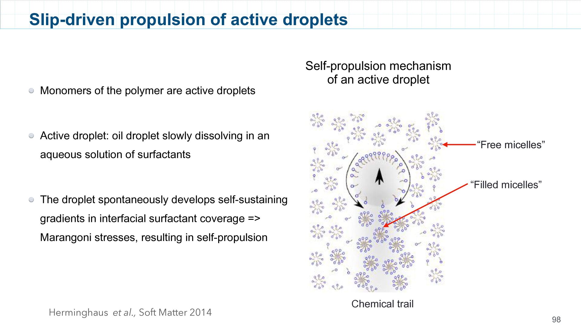
droplet slowly dissolving in an aqueous solution of surfactants The droplet spontaneously develops self-sustaining gradients in interfacial surfactant coverage => Marangoni stresses, resulting in self-propulsion 98 “Free micelles” Slip-driven propulsion of active droplets Herminghaus et al., Soft Matter 2014 “Filled micelles” “Free micelles” Chemical trail Self-propulsion mechanism of an active droplet
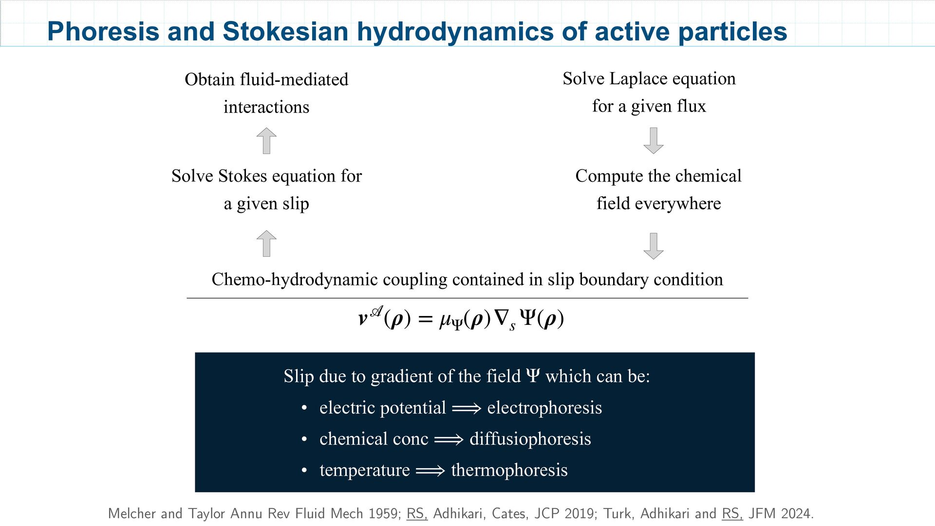
Cates, JCP 2019; Turk, Adhikari and RS, JFM 2024. Chemo-hydrodynamic coupling contained in slip boundary condition Solve Laplace equation for a given flux Obtain fluid-mediated interactions Compute the chemical field everywhere Solve Stokes equation for a given slip Phoresis and Stokesian hydrodynamics of active particles v (ρ) = μ Ψ (ρ)∇ s Ψ(ρ) Slip due to gradient of the field which can be: • electric potential electrophoresis • chemical conc diffusiophoresis • temperature thermophoresis Ψ ⟹ ⟹ ⟹
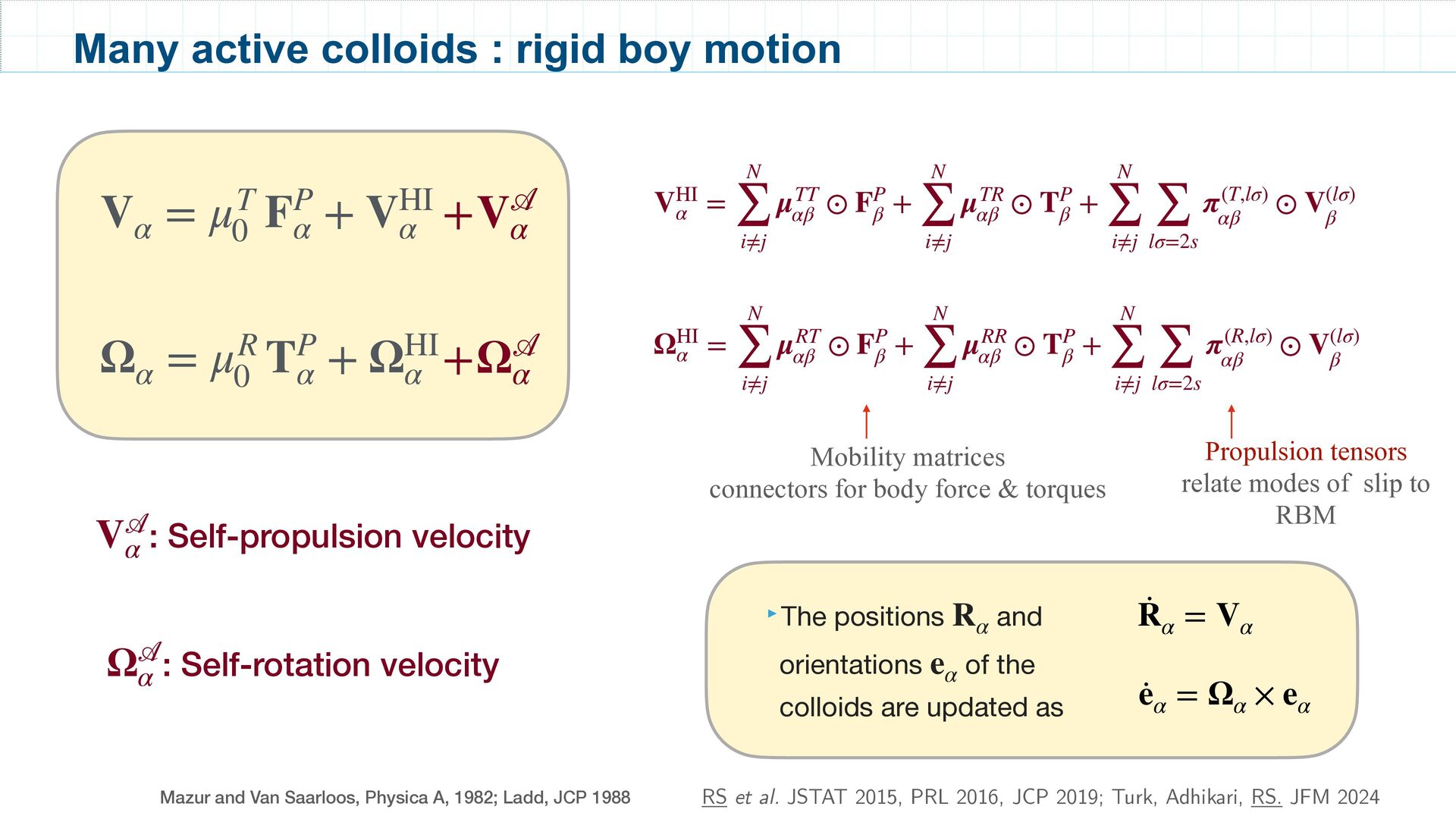
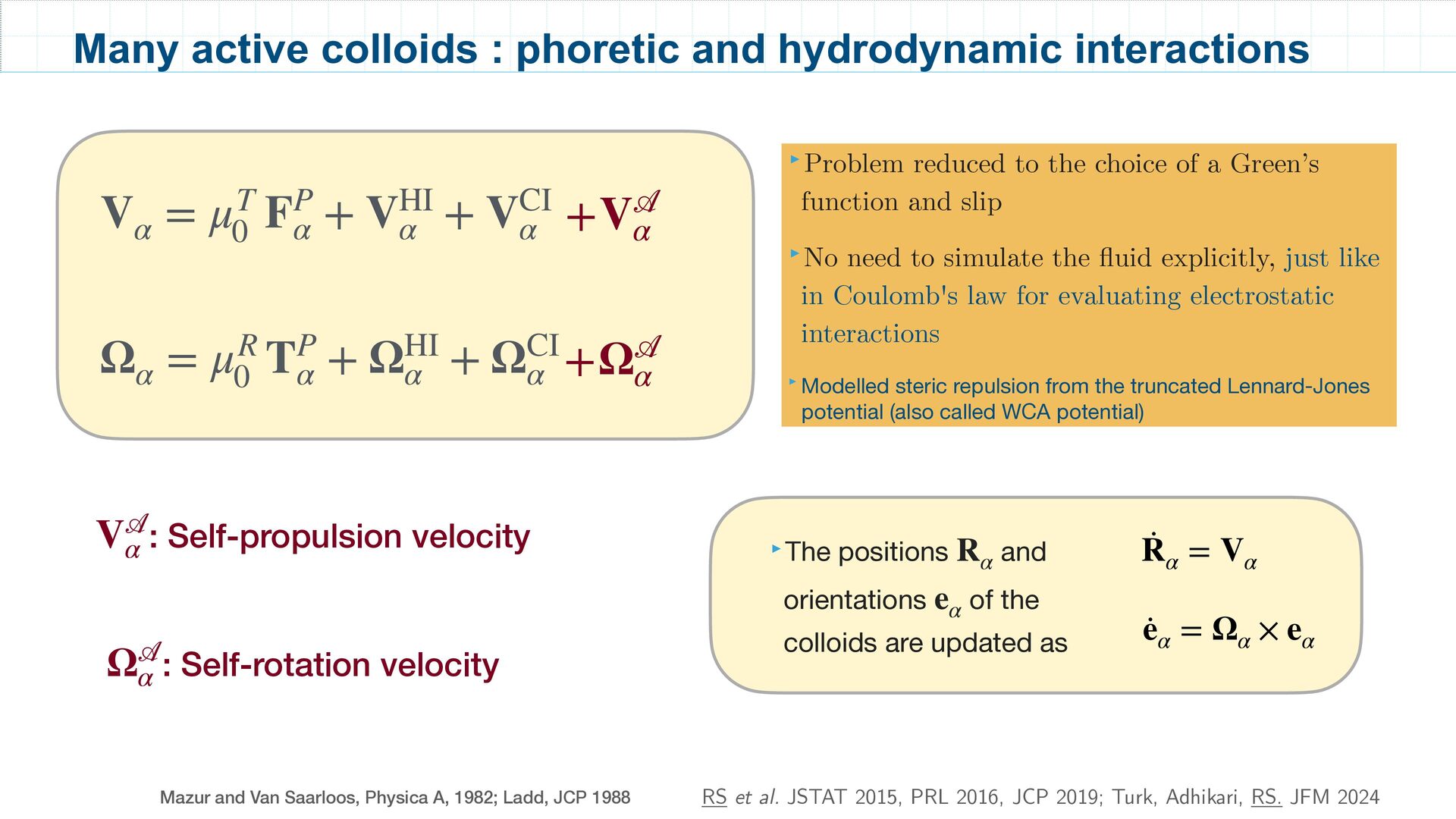
Van Saarloos, Physica A, 1982; Ladd, JCP 1988 V α = μT 0 FP α + VHI α + VCI α +V α Ω α = μR 0 TP α + ΩHI α + ΩCI α +Ω α : Self-propulsion velocity V α : Self-rotation velocity Ω α RS et al. JSTAT 2015, PRL 2016, JCP 2019; Turk, Adhikari, RS. JFM 2024 ‣Problem reduced to the choice of a Green’s function and slip ‣No need to simulate the fluid explicitly, just like in Coulomb's law for evaluating electrostatic interactions ‣Modelled steric repulsion from the truncated Lennard-Jones potential (also called WCA potential) ‣The positions and orientations of the colloids are updated as R α e α · R α = V α · e α = Ω α × e α
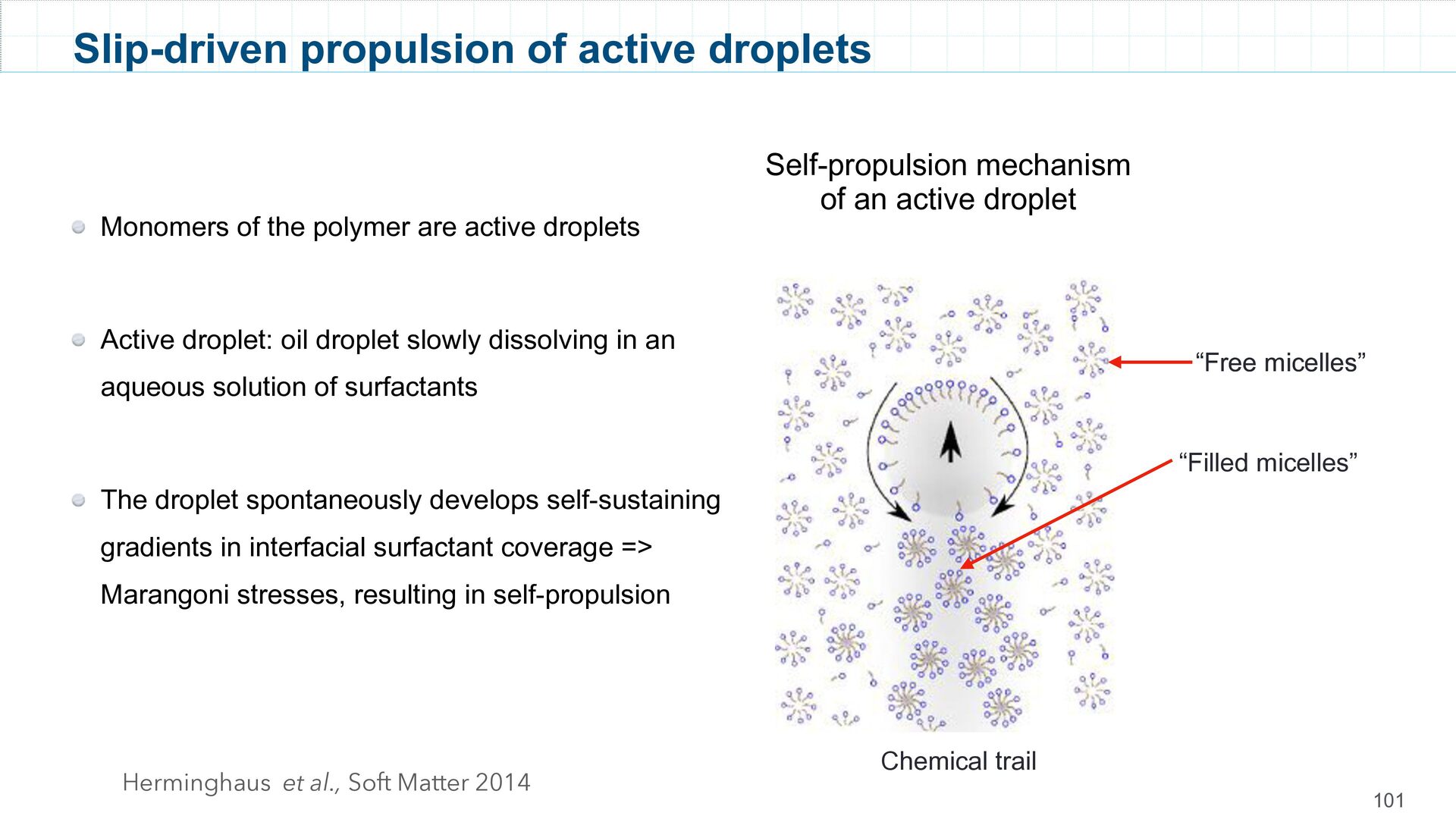
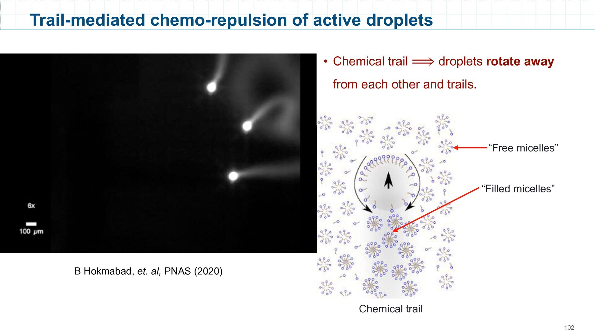
droplet slowly dissolving in an aqueous solution of surfactants The droplet spontaneously develops self-sustaining gradients in interfacial surfactant coverage => Marangoni stresses, resulting in self-propulsion 101 “Free micelles” Slip-driven propulsion of active droplets Herminghaus et al., Soft Matter 2014 “Filled micelles” “Free micelles” Chemical trail Self-propulsion mechanism of an active droplet
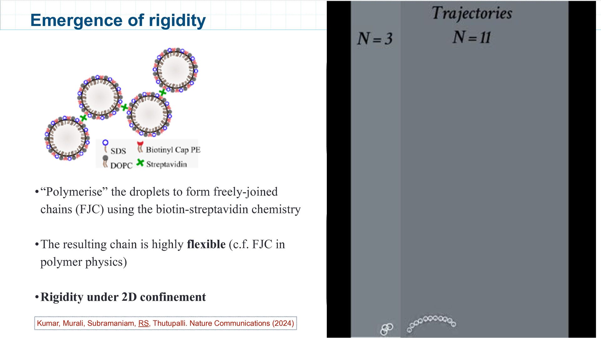
Communications (2024) Stabilisation into a C shape (Emergent rigidity) •“Polymerise” the droplets to form freely-joined chains (FJC) using the biotin-streptavidin chemistry •The resulting chain is highly flexible (c.f. FJC in polymer physics) •Rigidity under 2D confinement 103 Emergence of rigidity Dynamics in -plane xy
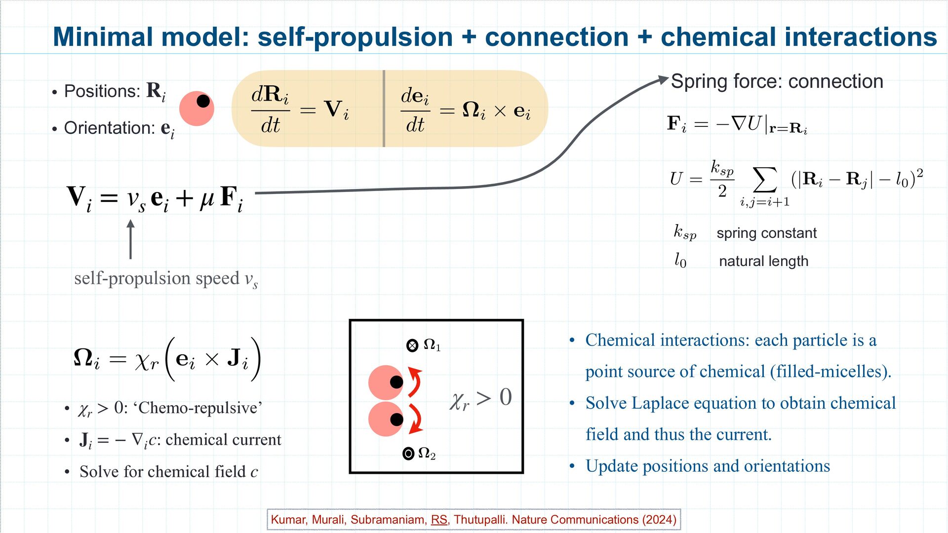
= Vi dei dt = ⌦i ⇥ ei • Chemical interactions: each particle is a point source of chemical (filled-micelles). • Solve Laplace equation to obtain chemical field and thus the current. • Update positions and orientations • Positions: • Orientation: R i e i ⌦i = r ⇣ ei ⇥ Ji ⌘ + p 2Dr⇠r self-propulsion speed v s Spring force: connection spring constant ksp Fi = rU|r=Ri natural length l0 U = ksp 2 X i,j=i+1 (|Ri Rj | l0)2 • : ‘Chemo-repulsive’ • : chemical current • Solve for chemical field χ r > 0 J i = − ∇ i c c <latexit sha1_base64="UMSPScrFYLvx+e5qgINNbQL8jV4=">AAAB/XicbVBPS8MwHE3nvzn/VXf0EhyCp9GOgR6HXrw5wTlhLSXN0i0sSUuSCqXUr+LFg4J49Xt489uYbj3o5oPA473fj9/LCxNGlXacb6u2tr6xuVXfbuzs7u0f2IdH9ypOJSYDHLNYPoRIEUYFGWiqGXlIJEE8ZGQYzq5Kf/hIpKKxuNNZQnyOJoJGFCNtpMBuehzpaRjl3g0nE1QEeacI7JbTduaAq8StSAtU6Af2lzeOccqJ0JghpUauk2g/R1JTzEjR8FJFEoRnaEJGhgrEifLzefgCnhplDKNYmic0nKu/N3LElcp4aCbLqGrZK8X/vFGqows/pyJJNRF4cShKGdQxLJuAYyoJ1iwzBGFJTVaIp0girE1fDVOCu/zlVTLstN1u23Vvu63eZdVHHRyDE3AGXHAOeuAa9MEAYJCBZ/AK3qwn68V6tz4WozWr2mmCP7A+fwCgsZU2</latexit> ⌦2 <latexit sha1_base64="sjAUCuhGvpCyWZRSy5tiS5Mt+EE=">AAAB+XicbVDLSsNAFL2pr1ofjbp0M1gEVyURQZdFNy4rWFtoQplMJ+3QyYOZG6GGfokbFwri1j9x5984abPQ1gMDh3Pu5Z45QSqFRsf5tipr6xubW9Xt2s7u3n7dPjh80EmmGO+wRCaqF1DNpYh5BwVK3ksVp1EgeTeY3BR+95ErLZL4Hqcp9yM6ikUoGEUjDey6F1EcB2HuoYi4ng3shtN05iCrxC1JA0q0B/aXN0xYFvEYmaRa910nRT+nCgWTfFbzMs1TyiZ0xPuGxtRc8fN58Bk5NcqQhIkyL0YyV39v5DTSehoFZrKIqZe9QvzP62cYXvm5iNMMecwWh8JMEkxI0QIZCsUZyqkhlClhshI2pooyNF3VTAnu8pdXSfe86V40XffuotG6LvuowjGcwBm4cAktuIU2dIBBBs/wCm/Wk/VivVsfi9GKVe4cwR9Ynz/zxpO+</latexit> ⇥ <latexit sha1_base64="p52XZ7L+hwZLv2j3Ueq3aJFOl5w=">AAAB/XicbVBPS8MwHE3nvzn/VXf0UhyCp9HIQI9DL96c4NxgLSXN0i0sSUuSCqXUr+LFg4J49Xt489uYbj3o5oPA473fj9/LCxNGlXbdb6u2tr6xuVXfbuzs7u0f2IdHDypOJSZ9HLNYDkOkCKOC9DXVjAwTSRAPGRmEs+vSHzwSqWgs7nWWEJ+jiaARxUgbKbCbHkd6Gka5d8vJBBVBDovAbrltdw5nlcCKtECFXmB/eeMYp5wIjRlSagTdRPs5kppiRoqGlyqSIDxDEzIyVCBOlJ/PwxfOqVHGThRL84R25urvjRxxpTIemskyqlr2SvE/b5Tq6NLPqUhSTQReHIpS5ujYKZtwxlQSrFlmCMKSmqwOniKJsDZ9NUwJcPnLq2Rw3oadNoR3nVb3quqjDo7BCTgDEFyALrgBPdAHGGTgGbyCN+vJerHerY/FaM2qdprgD6zPH58rlTU=</latexit> ⌦1 χ r > 0 V i = v s e i + μ F i Kumar, Murali, Subramaniam, RS, Thutupalli. Nature Communications (2024)
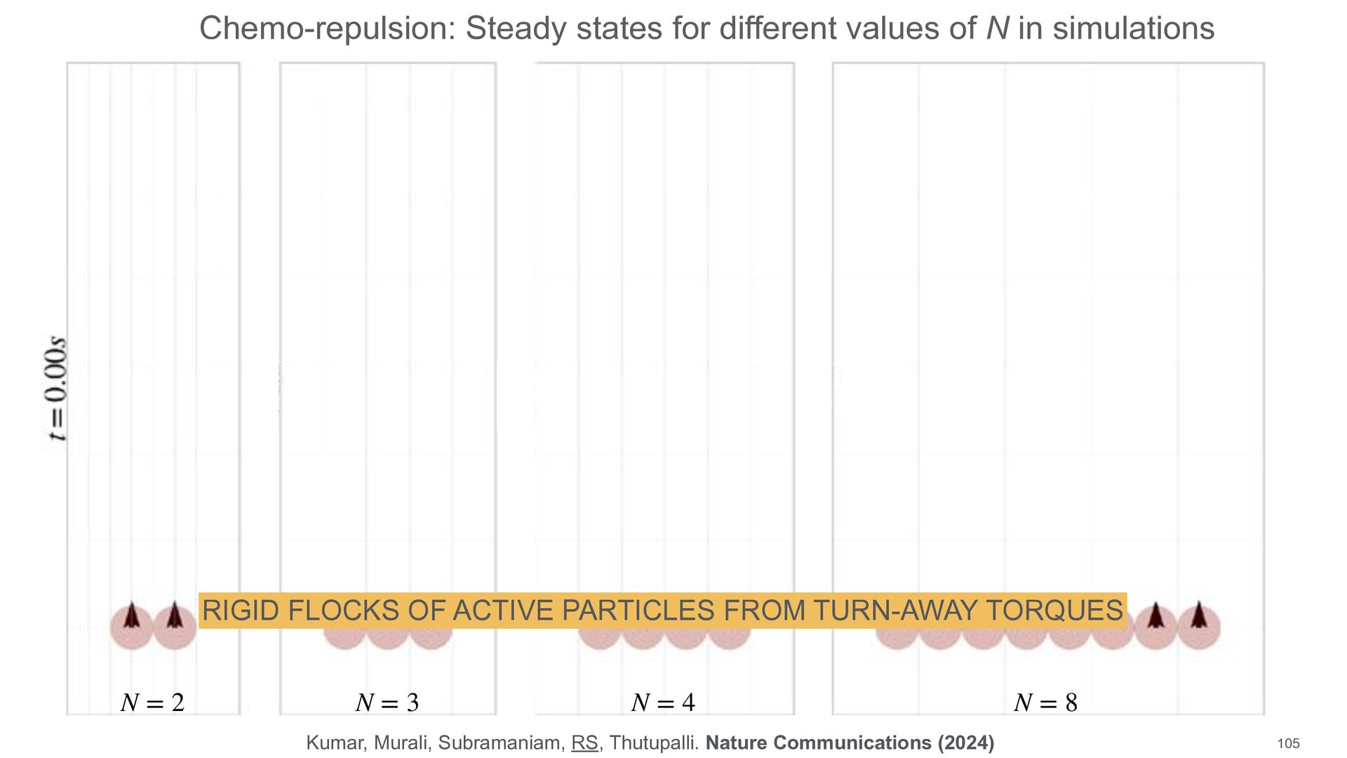
N = 4 N = 8 Chemo-repulsion: Steady states for different values of N in simulations Kumar, Murali, Subramaniam, RS, Thutupalli. Nature Communications (2024) 105 RIGID FLOCKS OF ACTIVE PARTICLES FROM TURN-AWAY TORQUES
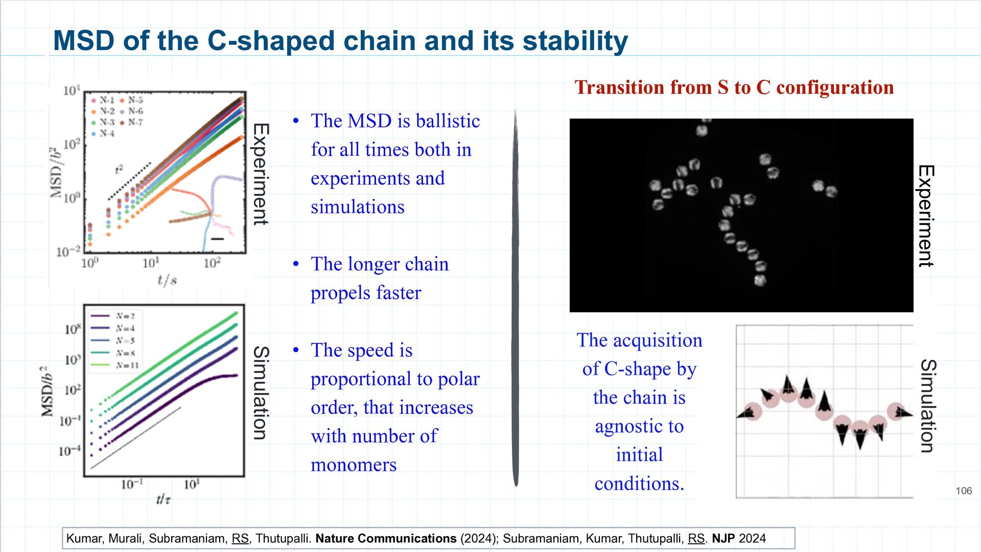
The MSD is ballistic for all times both in experiments and simulations • The longer chain propels faster • The speed is proportional to polar order, that increases with number of monomers Simulation Experiment Kumar, Murali, Subramaniam, RS, Thutupalli. Nature Communications (2024); Subramaniam, Kumar, Thutupalli, RS. NJP 2024 Simulation Experiment The acquisition of C-shape by the chain is agnostic to initial conditions. Transition from S to C configuration
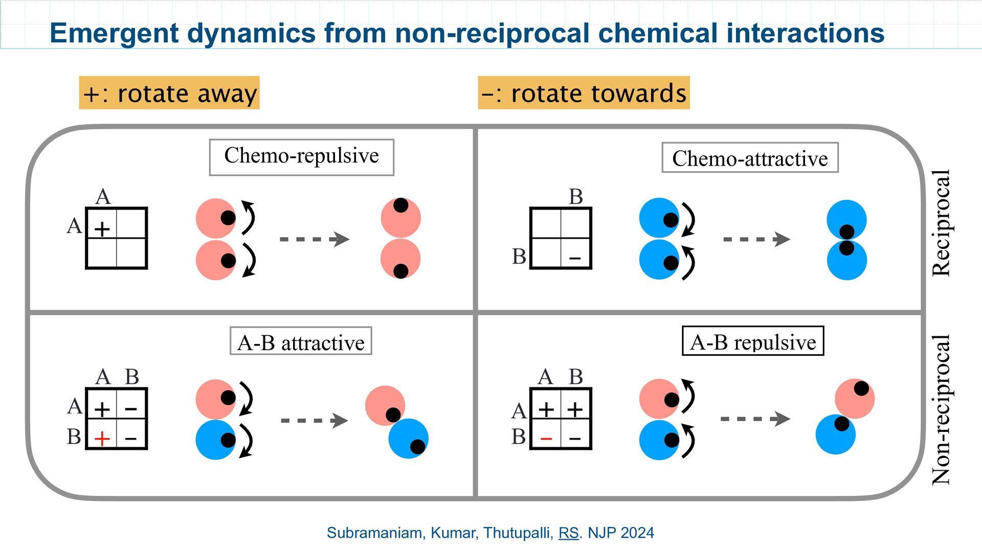
+ + - - A B A B - B B + A A A-B attractive Chemo-repulsive A-B repulsive Chemo-attractive Emergent dynamics from non-reciprocal chemical interactions Subramaniam, Kumar, Thutupalli, RS. NJP 2024 +: rotate away -: rotate towards


 rajeshrinet
 hanbao
 institutdelelevage
 tagtag
 rlifchitz
 sshimizu2006
.jpeg) arthur1
arthur1
 trycycle
 hayataka88
 lara
lara
 nikkihalliwell
 3n
3n
 carmenintech
 aleyda
 zakiyama
 tenderlove
 coloredviolet
 morganepeng
 sabderemane
 pwiseman
 cromwellryan