[ACCU2013] Measure and Manage Flow in Practice

Transcript

1. Measure and Manage Flow in Practice
   @ZsoltFabok
   http://zsoltfabok.com/
   by
   Zsolt Fabok
   2013-04-12
   Broke the WIP limit TWICE
   Still on the team
   #accu2013
   http://accu.org/index.php/conferences/accu_conference_2013/
   

   View Slide

2. 5 Stories from the life of a team by using
   real application and data
   The collected data is the courtesy of Digital Natives
   

   View Slide

3. #1 Too many open items
   

   View Slide

4. WIP
   point of observation
   Visualize the situation with
   Cumulative Flow Diagram
   solved
   

   View Slide

5. The Cumulative Flow Diagram
   Done
   Started
   Queued
   lead time
   cycle time
   WIP
   backlog
   time
   number of work items
   It offers more than just the WIP...
   

   View Slide

6. ~
   ~
   ~
   ~
   ~
   ~
   ~
   ~
   ~
   ~
   ~
   ~
   ~
   ~
   ~
   ~
   ~
   ~
   ~
   ~
   ~
   ~
   ~
   ~
   ~
   ~
   Q D
   3 4 1 2
   The simplest way of collecting data:
   

   View Slide

7. It is not easy to understand and
   see throughput from the CFD
   A quick detour:
   

   View Slide

8. work item
   WIP
   lead time
   /* detour */
   time
   

   View Slide

9. lead time
   work item
   throughput
   2
   WIP
   /* detour */
   

   View Slide

10. work item
    2 2
    /* detour */
    

    View Slide

11. Let’s add more people to the
    project so that “things speed up”!
    /* detour */
    

    View Slide

12. work item
    2 2 3
    coordination + communication cost
    /* detour */
    

    View Slide

13. Actually, “things slow down”, so it
    was not a good idea (solve the right
    problem instead - systems thinking).
    End of the detour.
    

    View Slide

14. #2 It takes too much
    time to deliver
    

    View Slide

15. lead time
    

    View Slide

16. lead time
    CFD was not much help here...
    ...because we didn’t know much about
    the nature of the lead time
    

    View Slide

17. Distribution of lead times
    days
    count
    0
    3
    5
    8
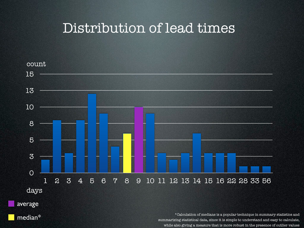
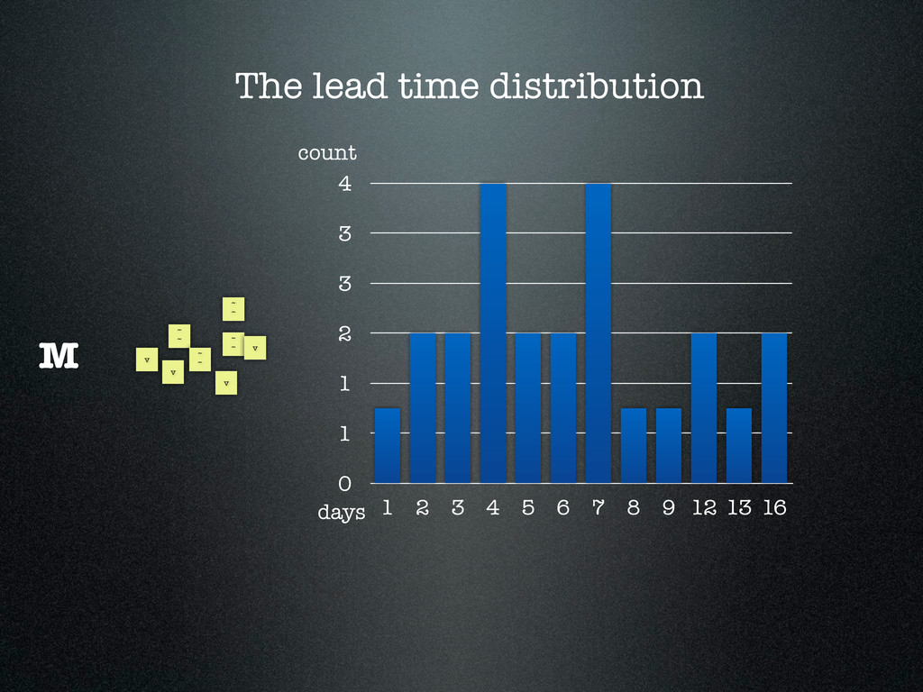
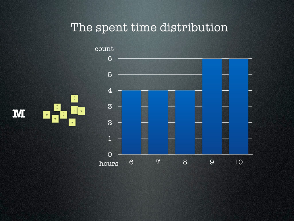
    10
    13
    15
    1 2 3 4 5 6 7 8 9 10 11 12 13 14 15 16 22 28 33 56
    average
    median* *Calculation of medians is a popular technique in summary statistics and
    summarizing statistical data, since it is simple to understand and easy to calculate,
    while also giving a measure that is more robust in the presence of outlier values
    

    View Slide

18. time spent on
    implementation
    (hours)
    time spent waiting
    (hours) %
    1 63 98
    7 57 90
    2 62 97
    2 62 97
    3 61 96
    Some examples of work items with 8-day
    lead time
    

    View Slide

19. View Slide

20. 95%
    of the lead
    time was spent
    on waiting
    

    View Slide

21. Distribution of lead times
    days
    count
    0
    3
    5
    8
    10
    13
    15
    1 4 7 10 13 16 33
    Before
    average
    0
    3
    5
    8
    10
    13
    15
    1 3 5 7 9 11 13 22
    count
    days
    After
    median
    

    View Slide

22. #3 Still too many open
    work items
    

    View Slide

23. How many
    times the item
    has been
    rejected
    

    View Slide

24. 0
    4
    8
    11
    15
    31-32 33-34 35-36 37-38
    Number of rejected work items
    count
    week
    

    View Slide

25. 0
    4
    8
    11
    15
    31-32 33-34 35-36 37-38 39-40 42-43 44-45
    Number of rejected work items
    count
    week
    

    View Slide

26. #4 Being predictable
    

    View Slide

27. Sales: “I want to know when the
    new features can hit the market!”
    Management: “I want to know
    how much it will cost me!”
    

    View Slide

28. All the work items we had so far
    (~20 work items)
    ~
    ~
    ~
    ~ ~
    ~
    ~
    ~
    ~
    ~
    ~
    ~
    v
    v
    v
    v
    v
    v
    v
    v
    

    View Slide

29. Categorizing them into three groups
    ~
    ~
    ~
    ~
    ~
    ~
    ~
    ~
    ~
    ~
    ~
    ~
    v
    v
    v
    v
    v
    v
    v
    v
    S
    M
    L
    

    View Slide

30. The lead time distribution
    ~
    ~
    ~
    ~
    ~
    ~
    ~
    ~
    v
    v
    v
    v
    M
    0
    1
    1
    2
    3
    3
    4
    1 2 3 4 5 6 7 8 9 12 13 16
    days
    count
    

    View Slide

31. The lead time distribution
    ~
    ~
    ~
    ~
    ~
    ~
    ~
    ~
    v
    v
    v
    v
    M
    0
    1
    1
    2
    3
    3
    4
    1 2 3 4 5 6 7 8 9 12 13 16
    SLA
    days
    count
    

    View Slide

32. The lead time distribution
    ~
    ~
    ~
    ~
    ~
    ~
    ~
    ~
    v
    v
    v
    v
    M
    0
    1
    1
    2
    3
    3
    4
    1 2 3 4 5 6 7 8 9 12 13 16
    SLA
    days
    count
    Expired
    

    View Slide

33. The spent time distribution
    ~
    ~
    ~
    ~
    ~
    ~
    ~
    ~
    v
    v
    v
    v
    M
    0
    1
    2
    3
    4
    5
    6
    6 7 8 9 10
    hours
    count
    

    View Slide

34. The spent time distribution
    ~
    ~
    ~
    ~
    ~
    ~
    ~
    ~
    v
    v
    v
    v
    M
    0
    1
    2
    3
    4
    5
    6
    6 7 8 9 10
    SLA
    hours
    count
    

    View Slide

35. View Slide

36. #5 Forced improvement
    

    View Slide

37. #1 We decided that we would
    force ourselves to keep the SLA
    #2 Nothing changed.
    Still the same ratio
    

    View Slide

38. Evolution of the
    team’s workflow
    

    View Slide

39. View Slide

40. View Slide

41. View Slide

42. Final thoughts on
    measurement
    

    View Slide

43. “If you can not measure it,
    you can not improve it.”
    Lord Kelvin
    image: http://en.wikipedia.org/wiki/File:Lord_Kelvin_photograph.jpg
    

    View Slide

44. “If you start measuring
    something you start
    optimizing it, and I know it's
    the wrong thing to optimize.”
    Paul Graham
    source: http://paulgraham.com/swan.html
    

    View Slide

45. image http://gjlh1249.wordpress.com/2011/03/20/waiting-for-the-bus/
    The bus stop effect
    

    View Slide

46. The Hawthorne Experiments
    (Elton Mayo, 1297) can
    explain the bus stop effect:
    Observation may influence
    the measurements.
    

    View Slide

47. “You can easily find data that
    perfectly suits your argument.”
    Zsolt Fabok
    (the handsome bloke who is standing in front of you)
    

    View Slide

48. Here is a good example
    

    View Slide

49. A sad data:
    “In 2011 drunk driving caused 15% of
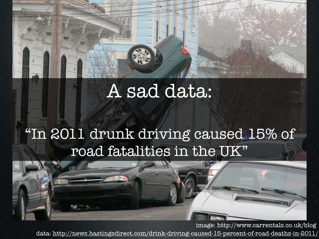
    road fatalities in the UK”
    data: http://news.hastingsdirect.com/drink-driving-caused-15-percent-of-road-deaths-in-2011/
    image: http://www.carrentals.co.uk/blog
    

    View Slide

50. If 15% of the road fatalities is
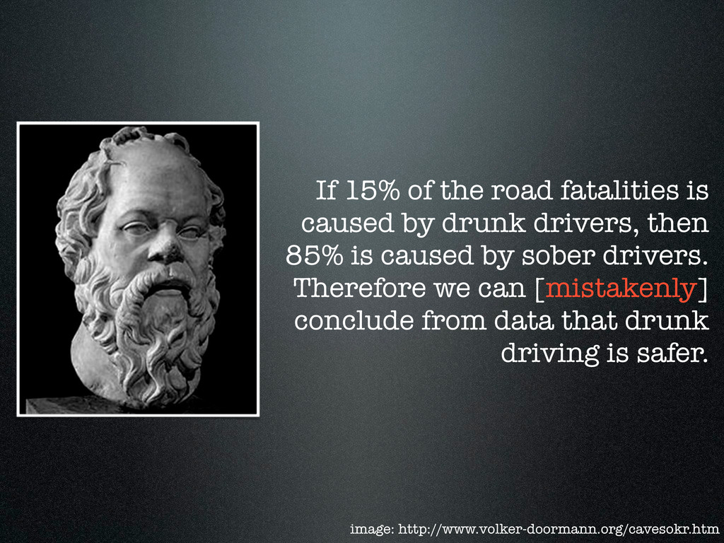
    caused by drunk drivers, then
    85% is caused by sober drivers.
    Therefore we can [mistakenly]
    conclude from data that drunk
    driving is safer.
    image: http://www.volker-doormann.org/cavesokr.htm
    

    View Slide

51. So let’s advise people to have at least
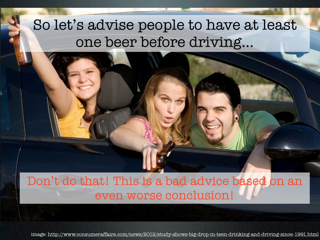
    one beer before driving...
    image: http://www.consumeraffairs.com/news/2012/study-shows-big-drop-in-teen-drinking-and-driving-since-1991.html
    Don’t do that! This is a bad advice based on an
    even worse conclusion!
    

    View Slide

52. The key ideas
    

    View Slide

53. 1. We develop software not models (value)
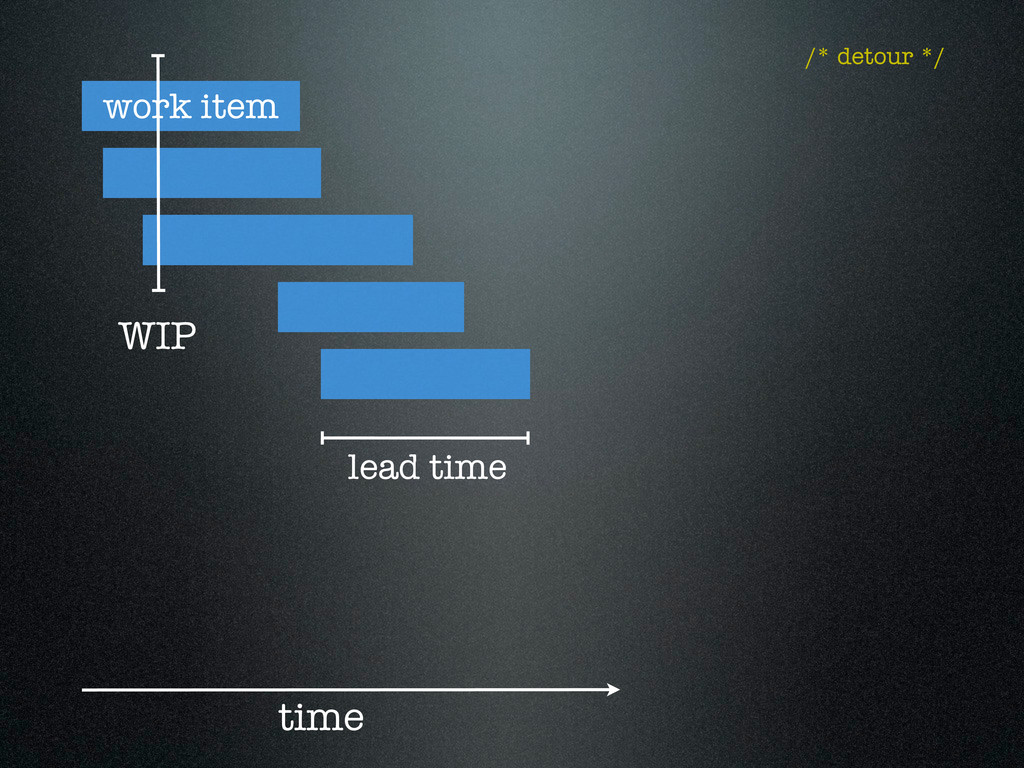
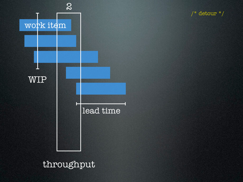
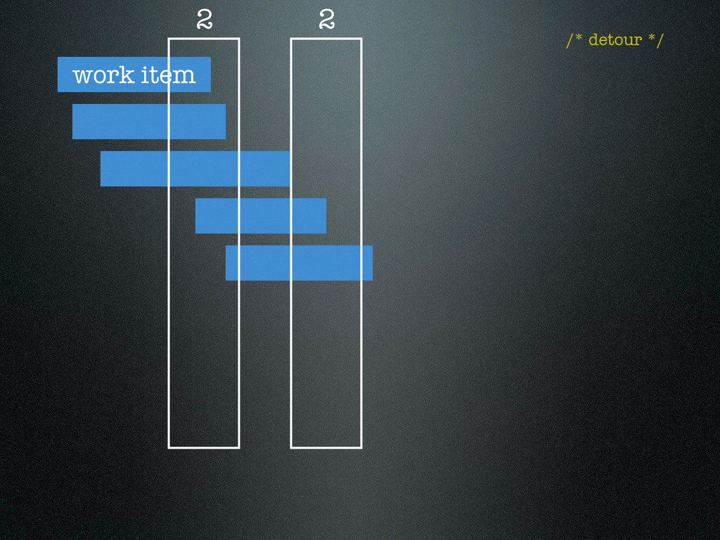
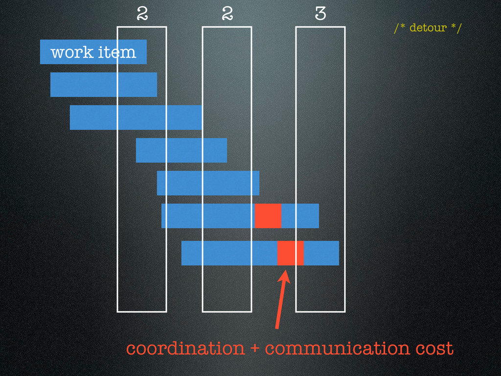
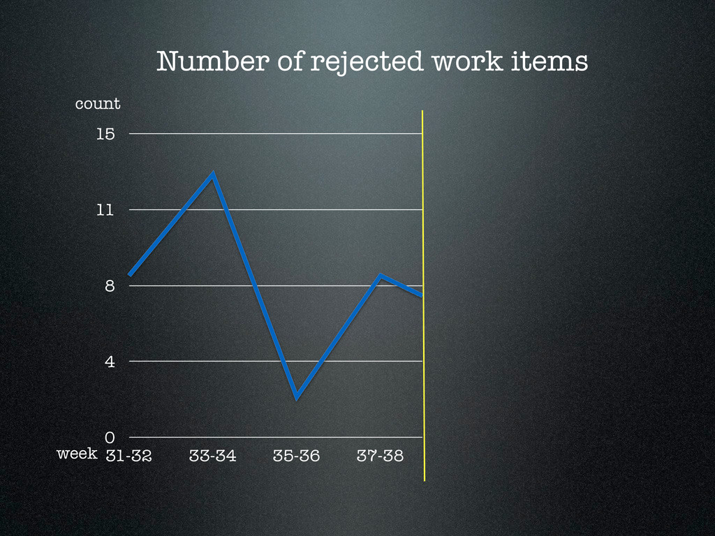
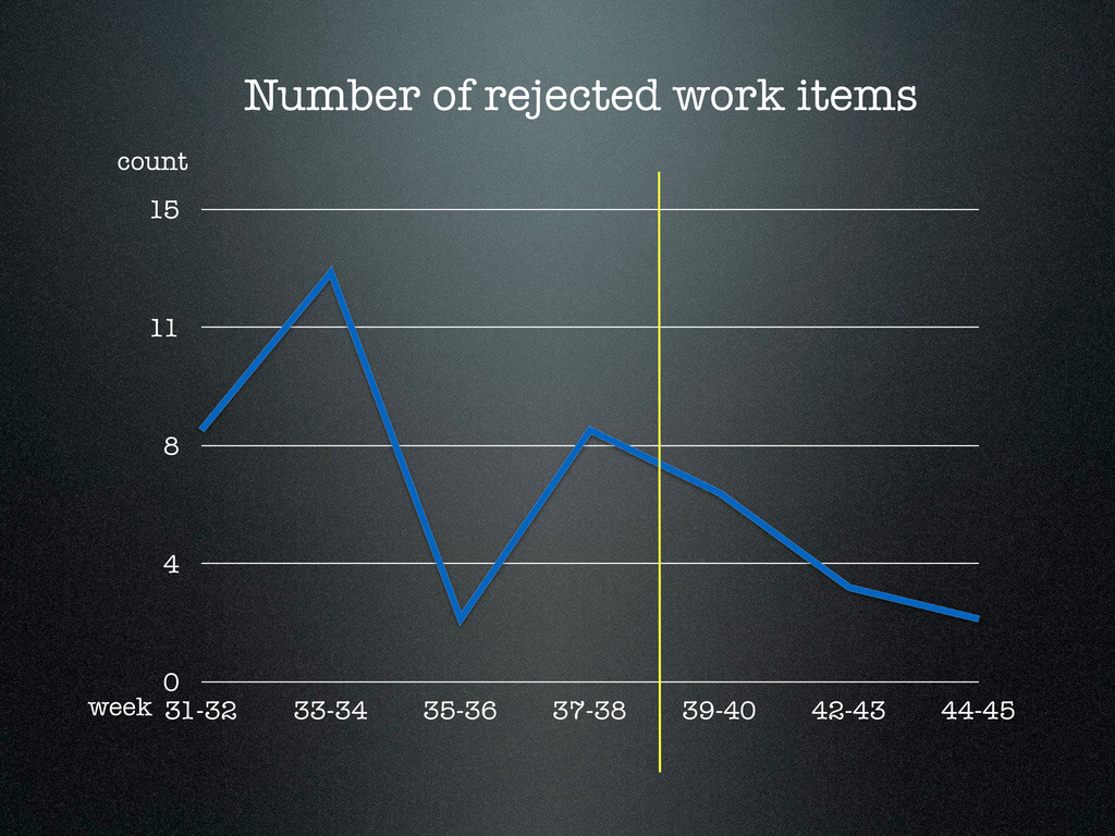
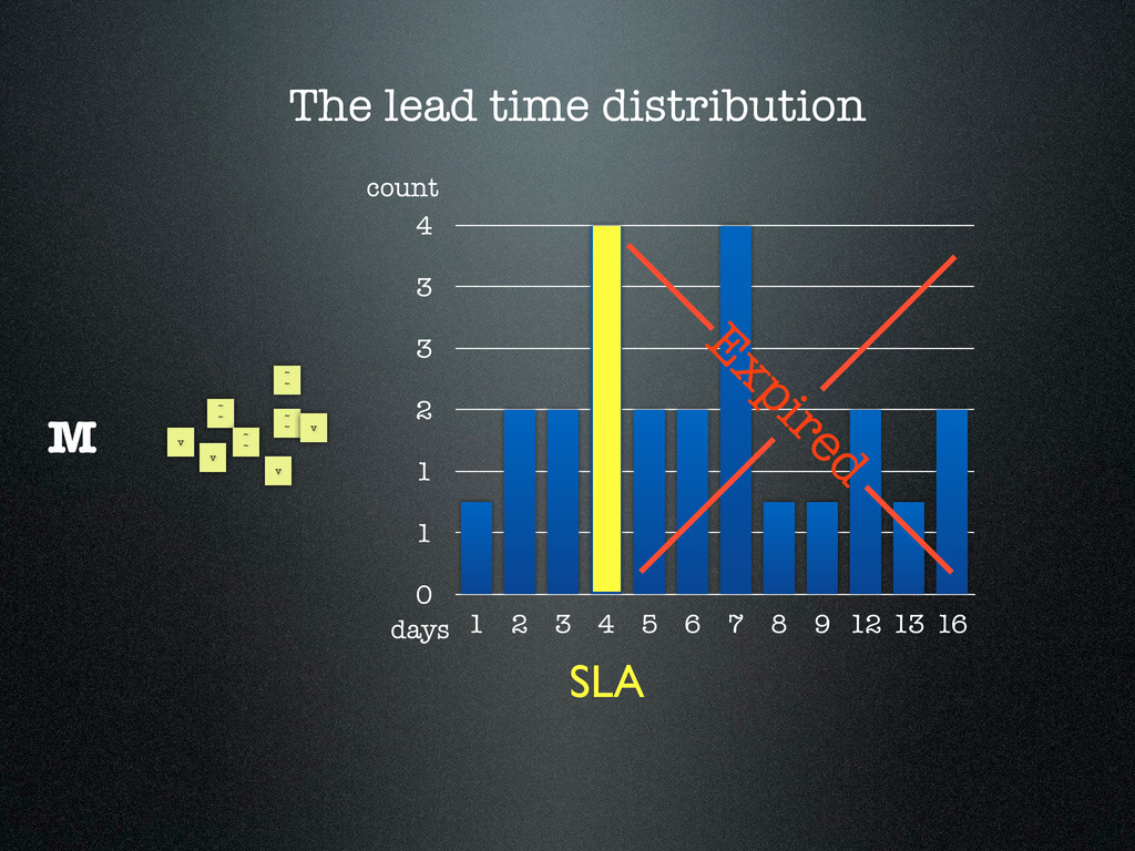
    2. Demand first, supply second
    3. Observe the system (lead time, throughput)
    4. Start measuring, look back if necessary
    5. Manage
    6. Mind that data expires
    7. Goto step 3.
    

    View Slide

54. Thank you very much for your attention!
    @ZsoltFabok
    http://zsoltfabok.com/
    

    View Slide