Hickernell SIAM UQ 2018 April Talk

Talk given at a SIAM UQ mini-symposium on probabilistic numerics

Transcript

1. Adaptive Bayesian Cubature Using Quasi-Monte Carlo Sequences Fred J. Hickernell & Jagadees Rathinavel Department of Applied Mathematics Center for Interdisciplinary Scientific Computation Illinois Institute of Technology hickernell@iit.edu mypages.iit.edu/~hickernell Thanks to the mini-symposium organizers, the GAIL team NSF-DMS-1522687 and NSF-DMS-1638521 (SAMSI) SIAM UQ 2018, April 17, 2018
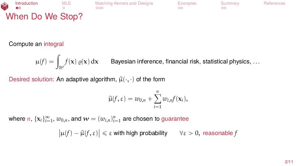
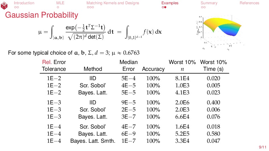
2. Introduction MLE Matching Kernels and Designs Examples Summary References When Do We Stop? Compute an integral µ(f) = ż Rd f(x) (x) dx Bayesian inference, financial risk, statistical physics, ... Desired solution: An adaptive algorithm, ^ µ(¨, ¨) of the form ^ µ(f, ε) = w0,n + n ÿ i=1 wi,n f(xi ), where n, txiu∞ i=1 , w0,n , and w = (wi,n )n i=1 are chosen to guarantee µ(f) ´ ^ µ(f, ε) ď ε with high probability @ε ą 0, reasonable f 2/11
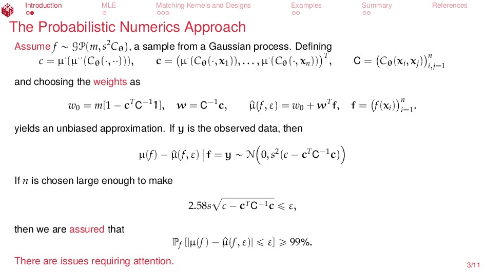
3. Introduction MLE Matching Kernels and Designs Examples Summary References The Probabilistic Numerics Approach Assume f „ GP(m, s2Cθ), a sample from a Gaussian process. Defining c = µ¨(µ¨¨(Cθ(¨, ¨¨))), c = µ¨(Cθ(¨, x1 )), . . . , µ¨(Cθ(¨, xn )) T , C = Cθ(xi , xj ) n i,j=1 and choosing the weights as w0 = m[1 ´ cTC´11], w = C´1c, ^ µ(f, ε) = w0 + wTf, f = f(xi ) n i=1 . yields an unbiased approximation. If y is the observed data, then µ(f) ´ ^ µ(f, ε) ˇ ˇ f = y „ N 0, s2(c ´ cTC´1c) If n is chosen large enough to make 2.58sac ´ cTC´1c ď ε, then we are assured that Pf [|µ(f) ´ ^ µ(f, ε)| ď ε] ě 99%. There are issues requiring attention. 3/11
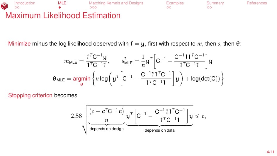
4. Introduction MLE Matching Kernels and Designs Examples Summary References Maximum Likelihood Estimation Minimize minus the log likelihood observed with f = y, first with respect to m, then s, then θ: mMLE = 1TC´1y 1TC´11 , s2 MLE = 1 n yT C´1 ´ C´111TC´1 1TC´11 y θMLE = argmin θ " n log yT C´1 ´ C´111TC´1 1TC´11 y + log(det(C)) * Stopping criterion becomes 2.58 g f f f f e c ´ cTC´1c n looooooomooooooon depends on design yT C´1 ´ C´111TC´1 1TC´11 y looooooooooooooomooooooooooooooon depends on data ď ε, 4/11
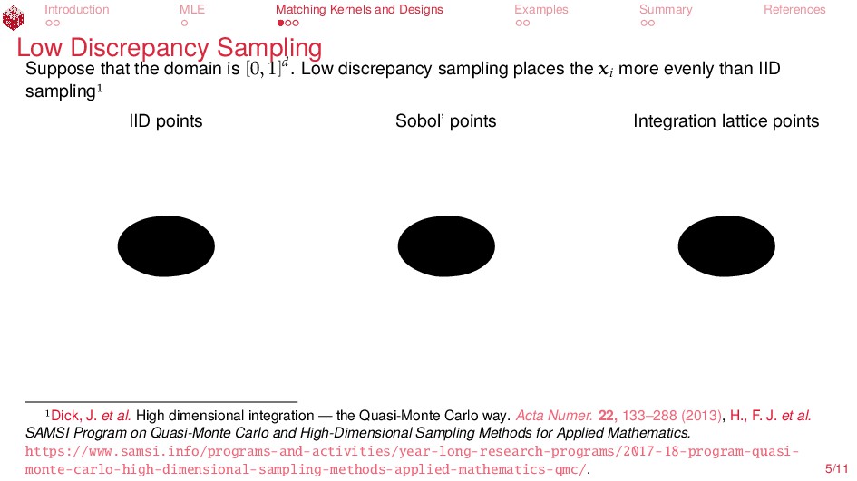
5. Introduction MLE Matching Kernels and Designs Examples Summary References Low Discrepancy Sampling Suppose that the domain is [0, 1]d. Low discrepancy sampling places the xi more evenly than IID sampling IID points Sobol’ points Integration lattice points ¨¨¨ Dick, J. et al. High dimensional integration — the Quasi-Monte Carlo way. Acta Numer. 22, 133–288 (2013), H., F. J. et al. SAMSI Program on Quasi-Monte Carlo and High-Dimensional Sampling Methods for Applied Mathematics. https://www.samsi.info/programs-and-activities/year-long-research-programs/2017-18-program-quasi- monte-carlo-high-dimensional-sampling-methods-applied-mathematics-qmc/. 5/11
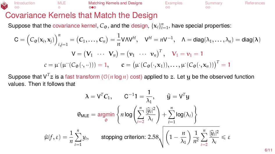
6. Introduction MLE Matching Kernels and Designs Examples Summary References Covariance Kernels that Match the Design Suppose that the covariance kernel, Cθ , and the design, txiun i=1 , have special properties: C = Cθ(xi , xj ) n i,j=1 = C1 , . . . , Cn = 1 n VΛVH, VH = nV´1, Λ = diag(λ1 , . . . , λn ) = diag(λ) V = V1 ¨ ¨ ¨ Vn = v1 ¨ ¨ ¨ vn T , V1 = v1 = 1 c = µ¨(µ¨¨(Cθ(¨, ¨¨))) = 1, c = µ¨(Cθ(¨, x1 )), . . . , µ¨(Cθ(¨, xn )) T = 1 Suppose that VTz is a fast transform (O(n log n) cost) applied to z. Let y be the observed function values. Then it follows that λ = VTC1 , C´11 = 1 λ1 , ^ y = VTy θMLE = argmin θ # n log n ÿ i=2 | p yi |2 λi + n ÿ i=1 log(λi ) + ^ µ(f, ε) = 1 n n ÿ i=1 yi , stopping criterion: 2.58 g f f e 1 ´ n λ1 1 n2 n ÿ i=2 | p yi |2 λi ď ε 6/11
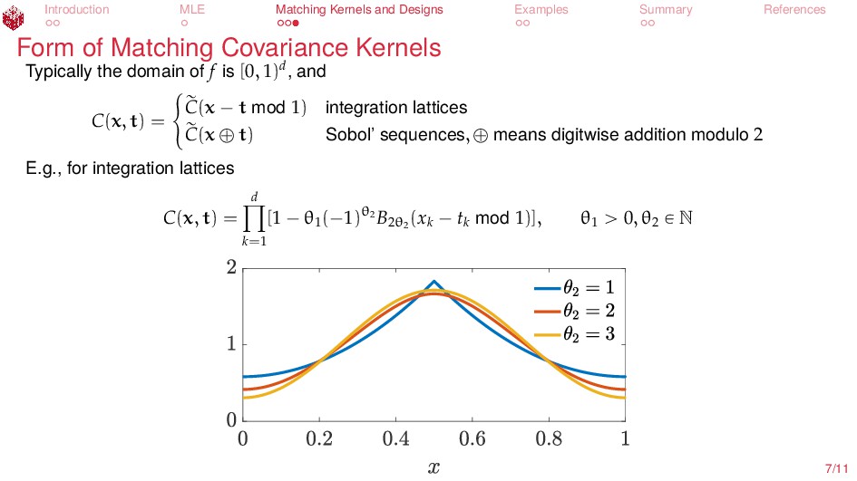
7. Introduction MLE Matching Kernels and Designs Examples Summary References Form of Matching Covariance Kernels Typically the domain of f is [0, 1)d, and C(x, t) = # r C(x ´ t mod 1) integration lattices r C(x ‘ t) Sobol’ sequences, ‘ means digitwise addition modulo 2 E.g., for integration lattices C(x, t) = d ź k=1 [1 ´ θ1 (´1)θ2 B2θ2 (xk ´ tk mod 1)], θ1 ą 0, θ2 P N 7/11
8. Introduction MLE Matching Kernels and Designs Examples Summary References Option Pricing µ = fair price = ż Rd e´rT max   1 d d ÿ j=1 Sj ´ K, 0   e´zTz/2 (2π)d/2 dz « $13.12 Sj = S0 e(r´σ2/2)jT/d+σxj = stock price at time jT/d, x = Az, AAT = Σ = min(i, j)T/d d i,j=1 , T = 1/4, d = 13 here Abs. Error Median Worst 10% Worst 10% Tolerance Method Error Accuracy n Time (s) 1E´2 IID diff 2E´3 100% 6.1E7 33.000 1E´2 Scr. Sobol’ PCA 1E´3 100% 1.6E4 0.040 1E´2 Scr. Sob. cont. var. PCA 2E´3 100% 4.1E3 0.019 1E´2 Bayes. Latt. PCA 2E´3 99% 1.6E4 0.051 8/11
9. Introduction MLE Matching Kernels and Designs Examples Summary References Gaussian Probability µ = ż [a,b] exp ´1 2 tTΣ´1t a(2π)d det(Σ) dt = ż [0,1]d´1 f(x) dx For some typical choice of a, b, Σ, d = 3; µ « 0.6763 Rel. Error Median Worst 10% Worst 10% Tolerance Method Error Accuracy n Time (s) 1E´2 IID 5E´4 100% 8.1E4 0.020 1E´2 Scr. Sobol’ 4E´5 100% 1.0E3 0.005 1E´2 Bayes. Latt. 5E´5 100% 4.1E3 0.023 1E´3 IID 9E´5 100% 2.0E6 0.400 1E´3 Scr. Sobol’ 2E´5 100% 2.0E3 0.006 1E´3 Bayes. Latt. 3E´7 100% 6.6E4 0.076 1E´4 Scr. Sobol’ 4E´7 100% 1.6E4 0.018 1E´4 Bayes. Latt. 6E´9 100% 5.2E5 0.580 1E´4 Bayes. Latt. Smth. 1E´7 100% 3.3E4 0.047 9/11
10. Introduction MLE Matching Kernels and Designs Examples Summary References Summary Bayesian cubature is successful as an automatic cuabature method We can handle relative and hybrid error tolerances? Matching the choice of kernels to the low discrepancy sequences makes the computation practical Need to explore how rich a family of kernels is needed in practice Need to explore when the Gaussian process assumption is reasonable For lattices need periodizing variable transformations to get higher order convergence For digital nets, higher order nets with the appropriate kernels should give higher order convergence Are their better alternatives to MLE for estimating parameters? 10/11
11. Thank you Slides available at www.slideshare.net/fjhickernell/hickernell-siam-uq-2018-april-talk
12. Introduction MLE Matching Kernels and Designs Examples Summary References Dick, J., Kuo, F. & Sloan, I. H. High dimensional integration — the Quasi-Monte Carlo way. Acta Numer. 22, 133–288 (2013). H., F. J., Kuo, F. Y., L’Ecuyer, P. & Owen, A. B. SAMSI Program on Quasi-Monte Carlo and High-Dimensional Sampling Methods for Applied Mathematics. https://www.samsi.info/programs-and-activities/year-long-research- programs/2017-18-program-quasi-monte-carlo-high-dimensional-sampling-methods- applied-mathematics-qmc/. 11/11