Dimensionality Reduction 101: PCA and PCoA

Transcript

1. Dimensionality Reduction 101: PCA & PCoA Gregory Ditzler Drexel University Dept. of Electrical & Computer Engineering Philadelphia, PA, 19104 gregory.ditzler@gmail.com http://github.com/gditzler/eces640-sklearn March 16, 2014
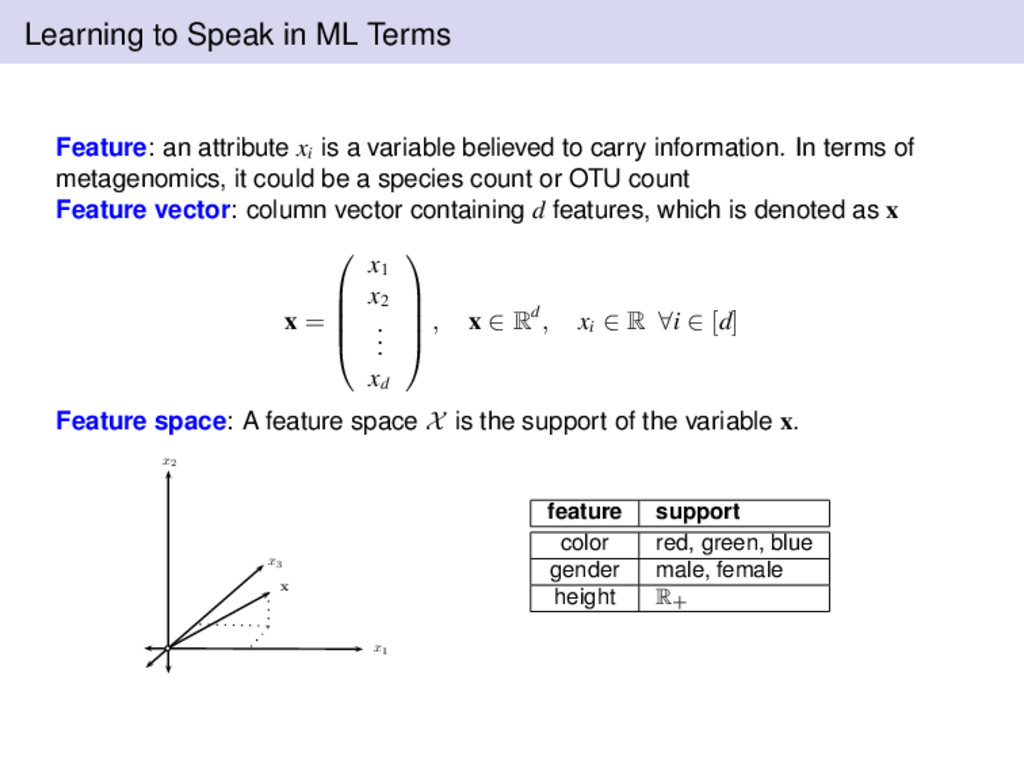
2. Learning to Speak in ML Terms Feature: an attribute xi is a variable believed to carry information. In terms of metagenomics, it could be a species count or OTU count Feature vector: column vector containing d features, which is denoted as x x =      x1 x2 . . . xd      , x ∈ Rd, xi ∈ R ∀i ∈ [d] Feature space: A feature space X is the support of the variable x. x3 x1 x2 x feature support color red, green, blue gender male, female height R+
3. Why should we reduce the dimensionality of the space? There is a curse of dimensionality! The complexity of a model increases with the dimensionality. Sometimes exponentially! So, why should we perform dimensionality reduction? reduces the time complexity: less computation reduces the space complexity: fewer parameters saves costs: some features/variables cost money makes interpreting complex high-dimensional data Can you visualize data with more than 3-dimensions?
4. Principal Components Analysis (PCA) Principal Components Analysis is an unsupervised dimensionality reduction technique Dimensionality of data may be large and many algorithms suffer from the curse of dimensionality Principal components maximize the variance (we will prove this!) Quite possibly the most popular dimensionality reduction method Mathematical tools needed: Eigenvalue problem, Lagrange multipliers, and a little bit about moments and variance. ⊗ ⊗ ⊗ ⊗ ⊗ ⊗ ⊗ ⊗ ⊗ ⊗ ⊗ ⊗ ⊗ ⊗ ⊗ ⊗ ⊗ ⊗ ⊗ ⊗ ⊗ ⊗ ⊗ ⊗ ⊗ ⊗ ⊗ ⊗ ⊗ ⊗ ⊗ ⊗ ⊗ ⊗ ⊗ ⊗ ⊗ ⊗ ⊗ ⊗ ⊗ ⊗ ⊗ ⊗ ⊗ ⊗ ⊗ ⊗ ⊗ ⊗ ⊗ e 1 2 3 4 5 6 7 8 9 10 −1 −2 −3 −4 −5 −6 −7 −8 −9 −10 1 2 3 4 5 6 7 8 9 10 −1 −2 −3 −4 −5 −6 −7 −8 −9 −10 ⊗ ⊗ ⊗ ⊗ ⊗ ⊗ ⊗ ⊗ ⊗ ⊗ ⊗ ⊗ ⊗ ⊗ ⊗ ⊗ ⊗ ⊗ ⊗ ⊗ ⊗ ⊗ ⊗ ⊗ ⊗ ⊗ ⊗ ⊗ ⊗ ⊗ ⊗ ⊗ ⊗ ⊗ ⊗ ⊗ ⊗ ⊗ ⊗ ⊗ ⊗ ⊗ ⊗ ⊗ ⊗ ⊗ ⊗ ⊗ ⊗ ⊗ ⊗ ⊗ ⊗ ⊗ ⊗ ⊗ ⊗ ⊗ ⊗ ⊗ ⊗ ⊗ ⊗ ⊗ ⊗ ⊗ ⊗ ⊗ ⊗ ⊗ ⊗ ⊗ ⊗ ⊗ ⊗ ⊗ ⊗ ⊗ ⊗ ⊗ ⊗ ⊗ ⊗ ⊗ ⊗ ⊗ ⊗ ⊗ ⊗ ⊗ ⊗ ⊗ ⊗ ⊗ ⊗ ⊗ ⊗ ⊗ ⊗ ⊗ ⊗ ⊗ ⊗ ⊗ ⊗ ⊗ ⊗ ⊗ ⊗ ⊗ ⊗ ⊗ ⊗ ⊗ ⊗ ⊗ ⊗ ⊗ ⊗ ⊗ ⊗ ⊗ ⊗ ⊗ ⊗ ⊗ ⊗ ⊗ ⊗ ⊗ ⊗ ⊗ ⊗ ⊗ ⊗ e =?
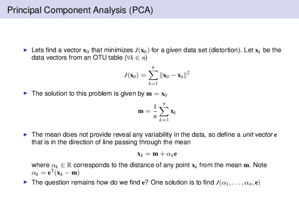
5. Principal Component Analysis (PCA) Lets find a vector x0 that minimizes J(x0) for a given data set (distortion). Let xk be the data vectors from an OTU table (∀k ∈ n) J(x0) = n k=1 x0 − xk 2 The solution to this problem is given by m = x0 m = 1 n n k=1 xk The mean does not provide reveal any variability in the data, so define a unit vector e that is in the direction of line passing through the mean xk = m + αke where αk ∈ R corresponds to the distance of any point xk from the mean m. Note αk = eT(xk − m) The question remains how do we find e? One solution is to find J(α1, . . . , αn, e)
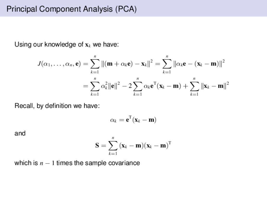
6. Principal Component Analysis (PCA) Using our knowledge of xk we have: J(α1 , . . . , αn , e) = n k=1 (m + αk e) − xk 2 = n k=1 αk e − (xk − m) 2 = n k=1 α2 k e 2 − 2 n k=1 αk eT(xk − m) + n k=1 xk − m 2 Recall, by definition we have: αk = eT(xk − m) and S = n k=1 (xk − m)(xk − m)T which is n − 1 times the sample covariance
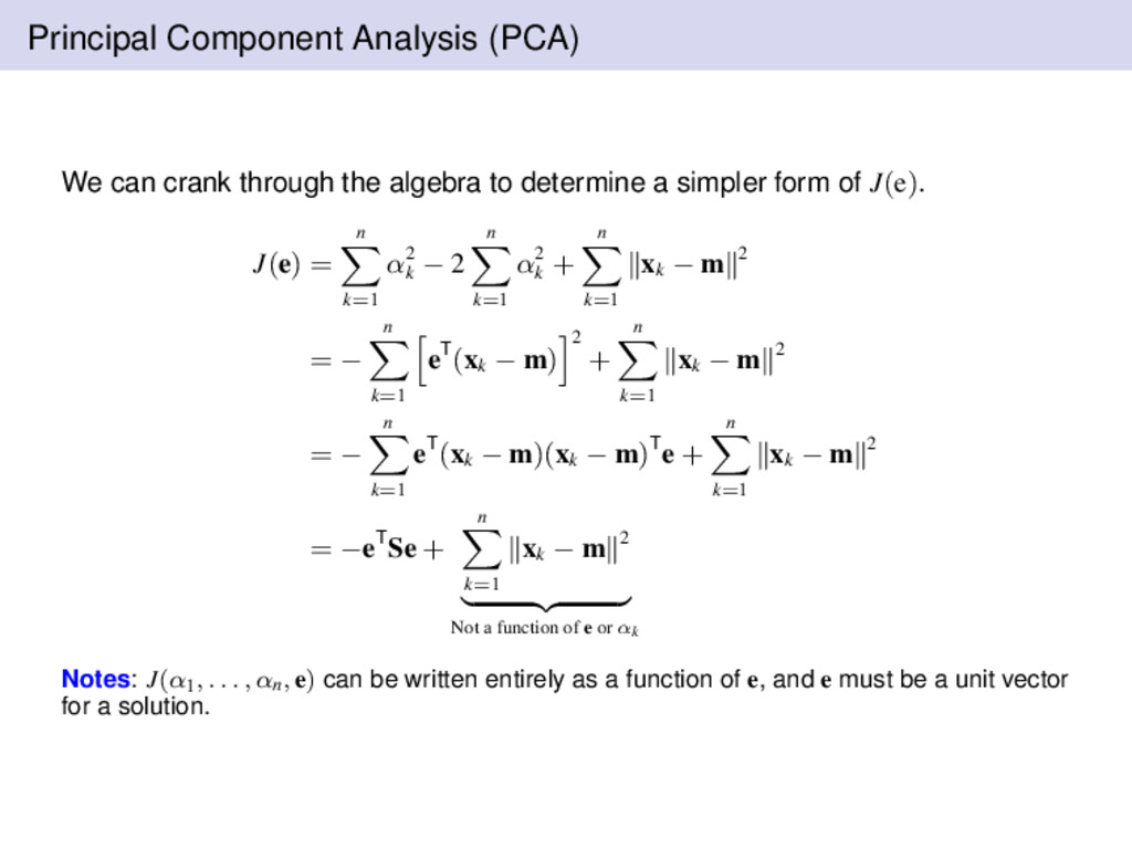
7. Principal Component Analysis (PCA) We can crank through the algebra to determine a simpler form of J(e). J(e) = n k=1 α2 k − 2 n k=1 α2 k + n k=1 xk − m 2 = − n k=1 eT(xk − m) 2 + n k=1 xk − m 2 = − n k=1 eT(xk − m)(xk − m)Te + n k=1 xk − m 2 = −eTSe + n k=1 xk − m 2 Not a function of e or αk Notes: J(α1, . . . , αn, e) can be written entirely as a function of e, and e must be a unit vector for a solution.
8. Principal Component Analysis (PCA) Minimizing −eTSe is equivalent to maximizing eTSe; however we are constrained to eTe − 1 = 0. The solution is quickly found via Lagrange multipliers. L(e, λ) = eTSe − λ(eTe − 1) Finding the maximum is simple since L(e, λ) is unconstrained. Simply take the derivative and set it equal to zero. ∂L ∂e = 2Se − 2λe = 0 ⇒ Se = λe Hence the solution vectors we are searching for are the eigenvectors of S.
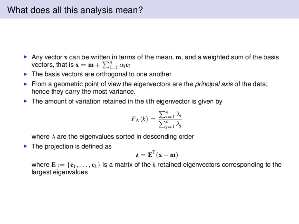
9. What does all this analysis mean? Any vector x can be written in terms of the mean, m, and a weighted sum of the basis vectors, that is x = m + n i=1 αiei The basis vectors are orthogonal to one another From a geometric point of view the eigenvectors are the principal axis of the data; hence they carry the most variance. The amount of variation retained in the kth eigenvector is given by FΛ(k) = k i=1 λi n j=1 λj where λ are the eigenvalues sorted in descending order The projection is defined as z = ET(x − m) where E := {e1, . . . , ek} is a matrix of the k retained eigenvectors corresponding to the largest eigenvalues
10. A few notes on PCA No class information is taken into account when we search for the principal axis The vector z is a combination of all the attributes in x because z is a projection The scatter matrix S ∈ Rd×d which makes solving Se = λe difficult for some problems Singular value decomposition (SVD) can be used, but we still are somewhat limited by large dimensional data sets Large d makes the solution nearly intractable even with SVD (as is the case in metagenomics) Other implementations of PCA: kernel and probabilistic KPCA: formulate PCA in terms of inner products PPCA: a set of observed data vectors may be determined through maximum-likelihood estimation of parameters in a latent variable model closely related to factor analysis PCA is also known as the discrete Karhunen–Lo´ eve transform
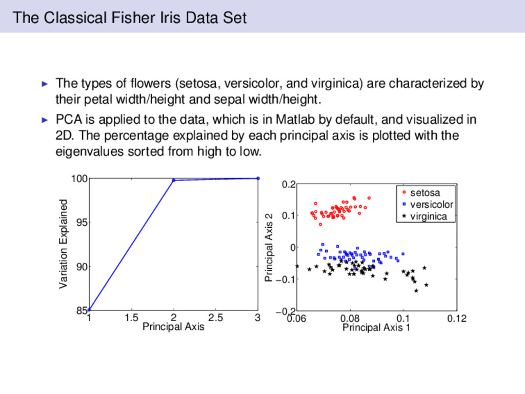
11. The Classical Fisher Iris Data Set The types of flowers (setosa, versicolor, and virginica) are characterized by their petal width/height and sepal width/height. PCA is applied to the data, which is in Matlab by default, and visualized in 2D. The percentage explained by each principal axis is plotted with the eigenvalues sorted from high to low. 1 1.5 2 2.5 3 85 90 95 100 Principal Axis Variation Explained 0.06 0.08 0.1 0.12 −0.2 −0.1 0 0.1 0.2 Principal Axis 1 Principal Axis 2 setosa versicolor virginica
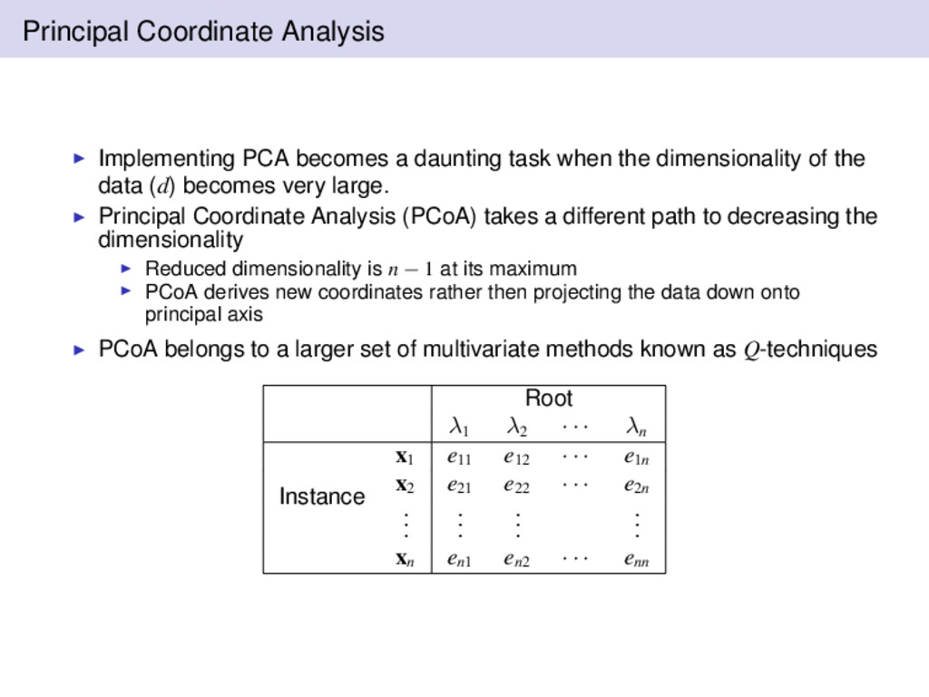
12. Principal Coordinate Analysis Implementing PCA becomes a daunting task when the dimensionality of the data (d) becomes very large. Principal Coordinate Analysis (PCoA) takes a different path to decreasing the dimensionality Reduced dimensionality is n − 1 at its maximum PCoA derives new coordinates rather then projecting the data down onto principal axis PCoA belongs to a larger set of multivariate methods known as Q-techniques Root λ1 λ2 · · · λn Instance x1 e11 e12 · · · e1n x2 e21 e22 · · · e2n . . . . . . . . . . . . xn en1 en2 · · · enn
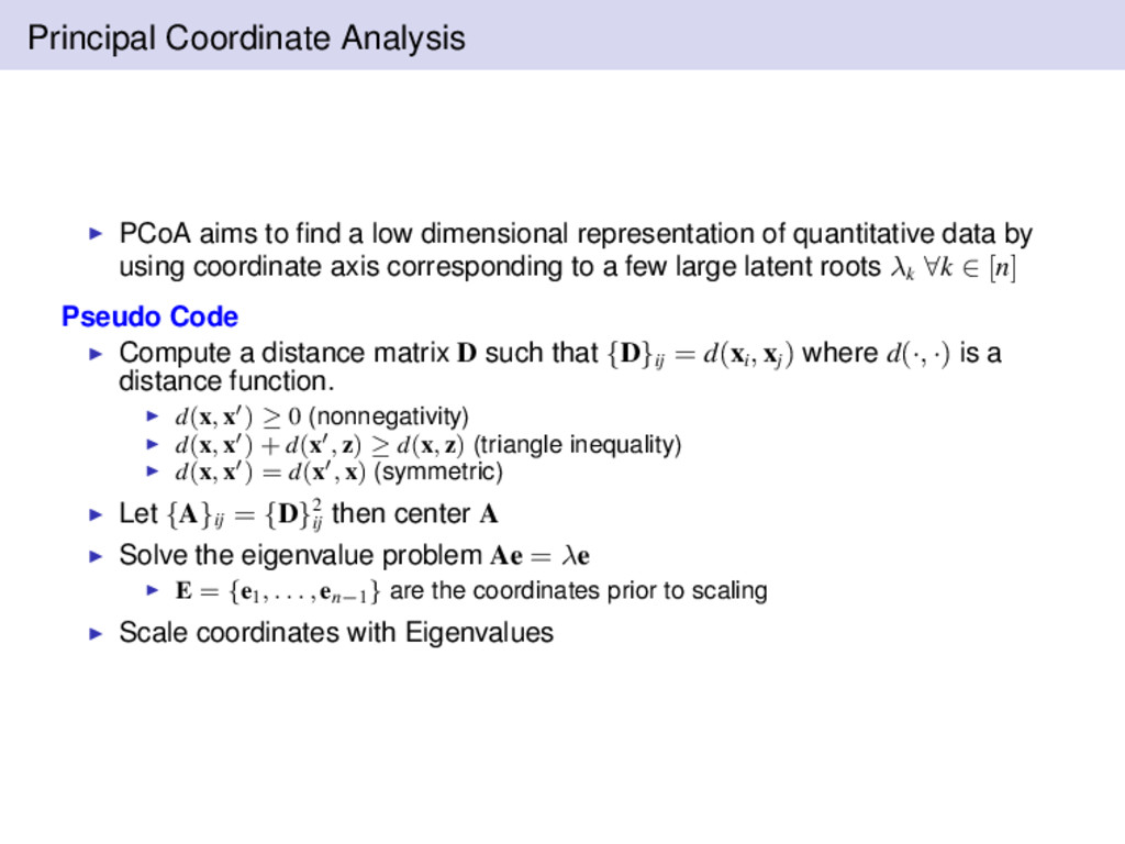
13. Principal Coordinate Analysis PCoA aims to find a low dimensional representation of quantitative data by using coordinate axis corresponding to a few large latent roots λk ∀k ∈ [n] Pseudo Code Compute a distance matrix D such that {D}ij = d(xi , xj ) where d(·, ·) is a distance function. d(x, x ) ≥ 0 (nonnegativity) d(x, x ) + d(x , z) ≥ d(x, z) (triangle inequality) d(x, x ) = d(x , x) (symmetric) Let {A}ij = {D}2 ij then center A Solve the eigenvalue problem Ae = λe E = {e1, . . . , en−1} are the coordinates prior to scaling Scale coordinates with Eigenvalues
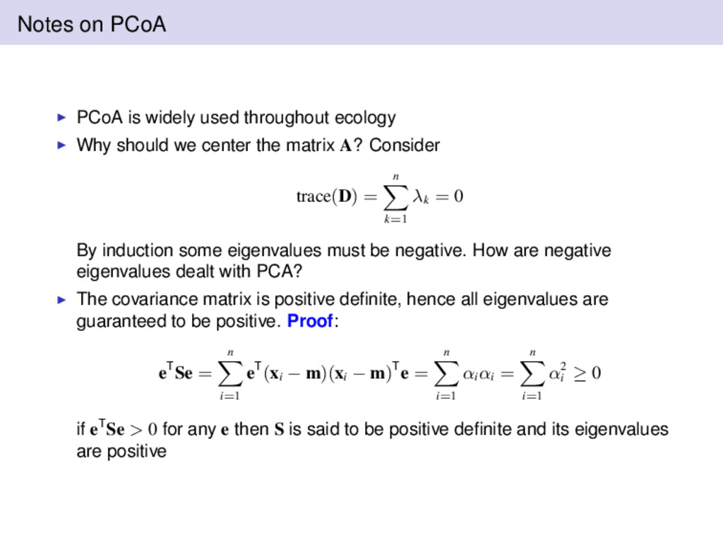
14. Notes on PCoA PCoA is widely used throughout ecology Why should we center the matrix A? Consider trace(D) = n k=1 λk = 0 By induction some eigenvalues must be negative. How are negative eigenvalues dealt with PCA? The covariance matrix is positive definite, hence all eigenvalues are guaranteed to be positive. Proof: eTSe = n i=1 eT(xi − m)(xi − m)Te = n i=1 αi αi = n i=1 α2 i ≥ 0 if eTSe > 0 for any e then S is said to be positive definite and its eigenvalues are positive
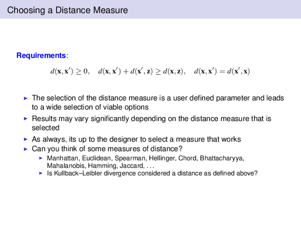
15. Choosing a Distance Measure Requirements: d(x, x ) ≥ 0, d(x, x ) + d(x , z) ≥ d(x, z), d(x, x ) = d(x , x) The selection of the distance measure is a user defined parameter and leads to a wide selection of viable options Results may vary significantly depending on the distance measure that is selected As always, its up to the designer to select a measure that works Can you think of some measures of distance? Manhattan, Euclidean, Spearman, Hellinger, Chord, Bhattacharyya, Mahalanobis, Hamming, Jaccard, . . . Is Kullback–Leibler divergence considered a distance as defined above?
16. A Few Common Distance Measures Euclidean d2(x, x ) = x − x 2 Manhattan dM (x, x ) = d i=1 |xi − xi | Bray-Curtis dB (x, x ) = 2Cij Si + Sj Hellinger dH (x, x ) = 1 d d i=1 xi |x| − xi |x | 2
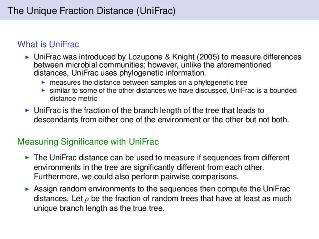
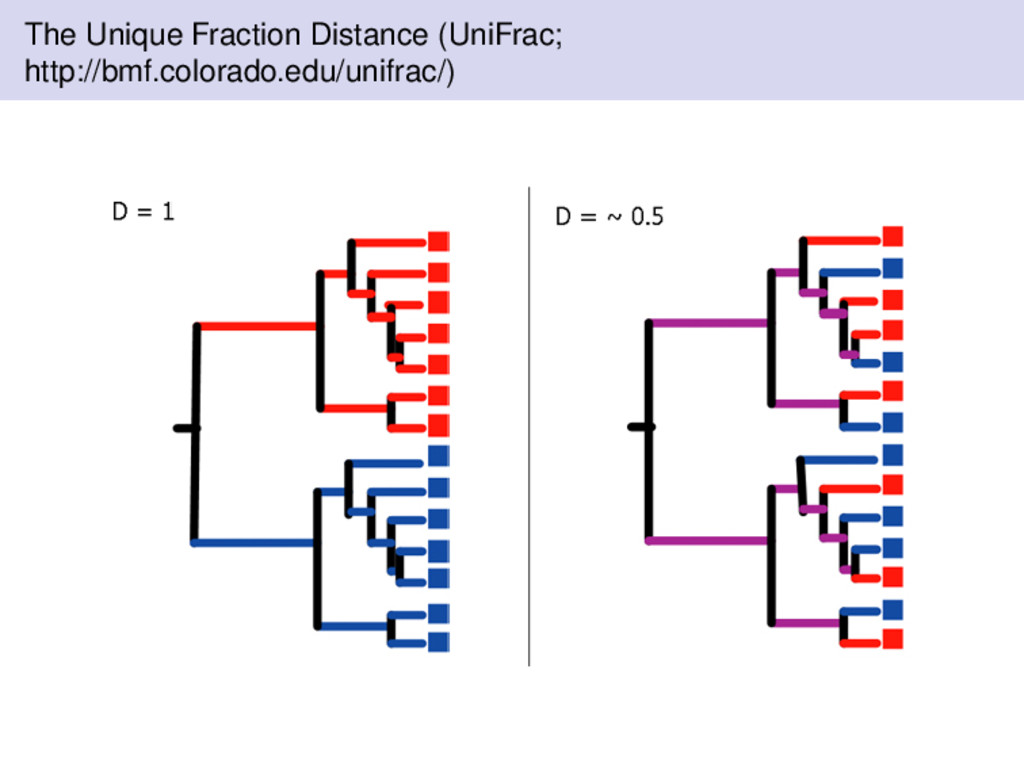
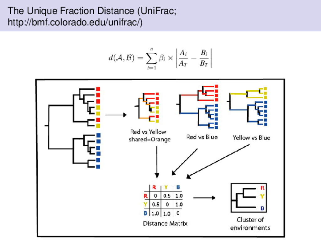
17. The Unique Fraction Distance (UniFrac) What is UniFrac UniFrac was introduced by Lozupone & Knight (2005) to measure differences between microbial communities; however, unlike the aforementioned distances, UniFrac uses phylogenetic information. measures the distance between samples on a phylogenetic tree similar to some of the other distances we have discussed, UniFrac is a bounded distance metric UniFrac is the fraction of the branch length of the tree that leads to descendants from either one of the environment or the other but not both. Measuring Significance with UniFrac The UniFrac distance can be used to measure if sequences from different environments in the tree are significantly different from each other. Furthermore, we could also perform pairwise comparisons. Assign random environments to the sequences then compute the UniFrac distances. Let p be the fraction of random trees that have at least as much unique branch length as the true tree.
18. The Unique Fraction Distance (UniFrac; http://bmf.colorado.edu/unifrac/)
19. The Unique Fraction Distance (UniFrac; http://bmf.colorado.edu/unifrac/) d(A, B) = n i=1 βi × Ai AT − Bi BT
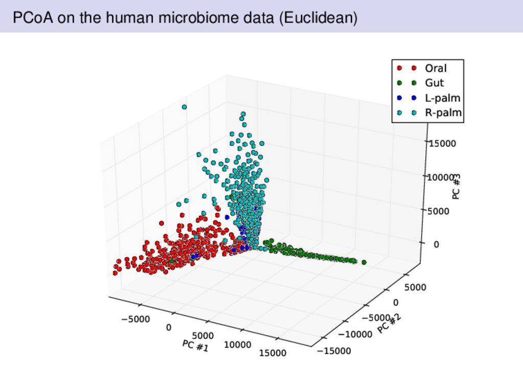
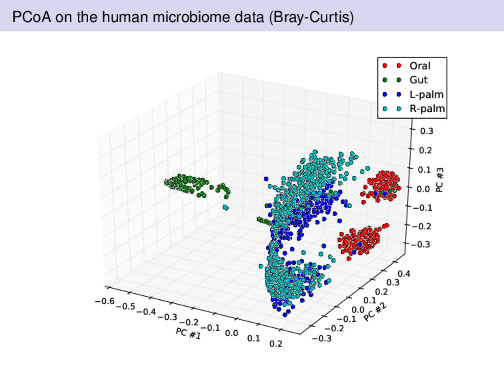
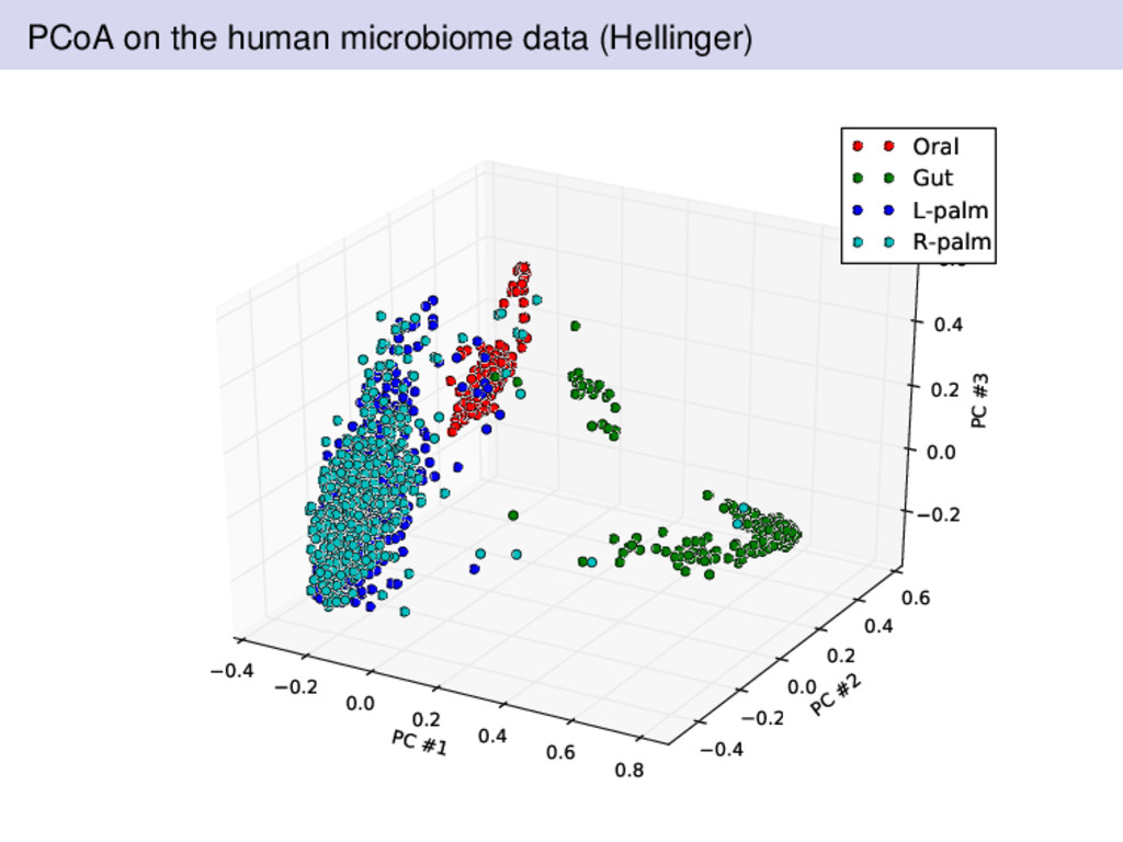
20. PCoA on the human microbiome data Metagenomic samples were collected from two individuals over a 15 month period by Rob Knight’s lab in Colorado A healthy female and male volunteered for data collected Sampling was performed at four body sites left palm, right palm, gut, and tongue Subjects are sampled regularly Where should we expect there to be differences? What was different about the Bray-Curtis dissimilarity compared to Euclidean or Hellinger distances?
21. PCoA on the human microbiome data (Euclidean) PC #1 5000 0 5000 10000 15000 PC #2 15000 10000 5000 0 5000 PC #3 0 5000 10000 15000 Oral Gut L-palm R-palm
22. PCoA on the human microbiome data (Bray-Curtis) PC #1 0.6 0.5 0.4 0.3 0.2 0.1 0.0 0.1 0.2 PC #2 0.3 0.2 0.1 0.0 0.1 0.2 0.3 0.4 PC #3 0.3 0.2 0.1 0.0 0.1 0.2 0.3 Oral Gut L-palm R-palm
23. PCoA on the human microbiome data (Hellinger) PC #1 0.4 0.2 0.0 0.2 0.4 0.6 0.8 PC #2 0.4 0.2 0.0 0.2 0.4 0.6 PC #3 0.2 0.0 0.2 0.4 0.6 Oral Gut L-palm R-palm
24. Demo Time! Seriously through, next time you’re in the Python shell, run >>>> import antigravity