University Ecological and Evolutionary Signal Processing & Informatics Lab Department of Electrical & Computer Engineering Philadelphia, PA, USA [email protected] http://github.com/gditzler/eces436-week1 April 1, 2014
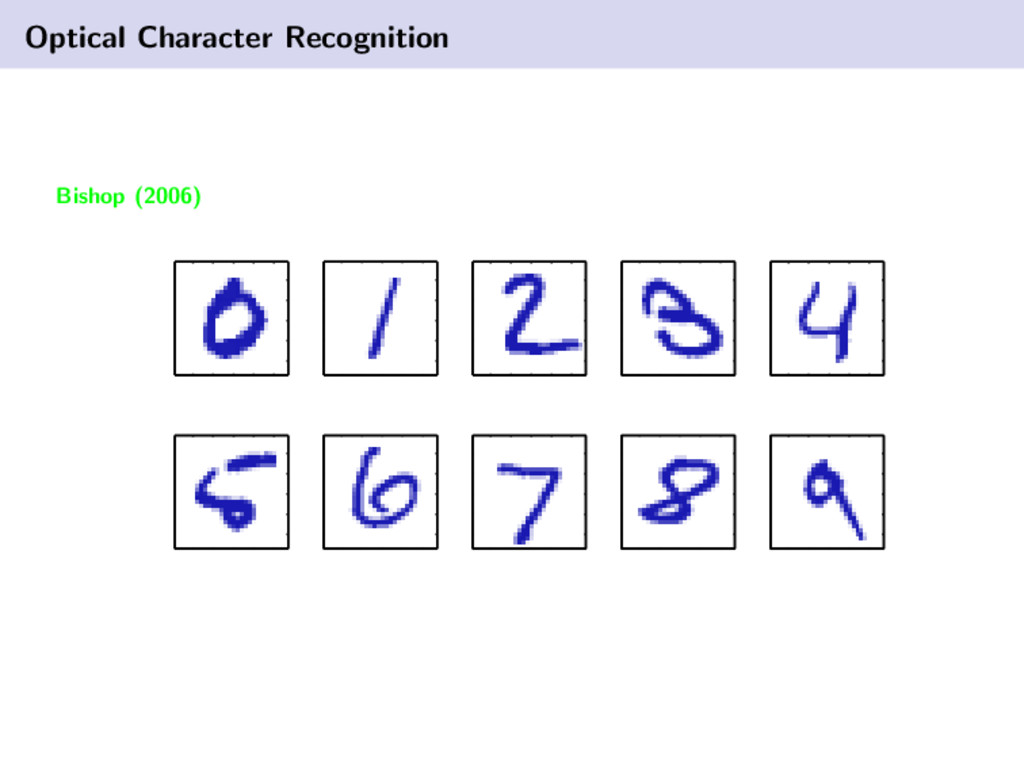
Image Rights Many of the images used in this presentation are from Christopher M. Bishop’s “Pattern Recognition and Machine Learning” (2006) text book. http://research.microsoft.com/en-us/um/people/cmbishop/prml/index.htm
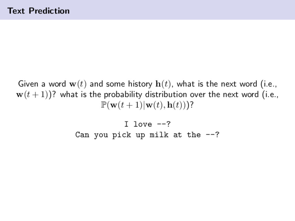
what is the next word (i.e., w(t + 1))? what is the probability distribution over the next word (i.e., P(w(t + 1)|w(t), h(t)))? I love --? Can you pick up milk at the --?
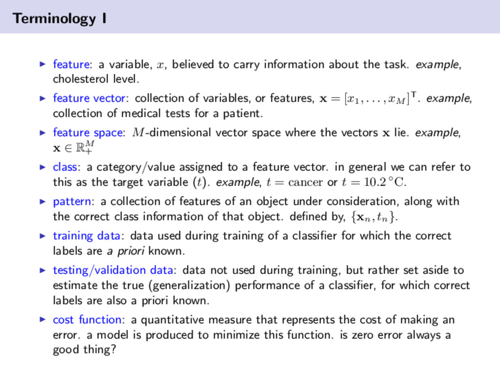
about the task. example, cholesterol level. feature vector: collection of variables, or features, x = [x1 , . . . , xM ]T. example, collection of medical tests for a patient. feature space: M-dimensional vector space where the vectors x lie. example, x ∈ RM + class: a category/value assigned to a feature vector. in general we can refer to this as the target variable (t). example, t = cancer or t = 10.2 ◦C. pattern: a collection of features of an object under consideration, along with the correct class information of that object. defined by, {xn , tn }. training data: data used during training of a classifier for which the correct labels are a priori known. testing/validation data: data not used during training, but rather set aside to estimate the true (generalization) performance of a classifier, for which correct labels are also a priori known. cost function: a quantitative measure that represents the cost of making an error. a model is produced to minimize this function. is zero error always a good thing?
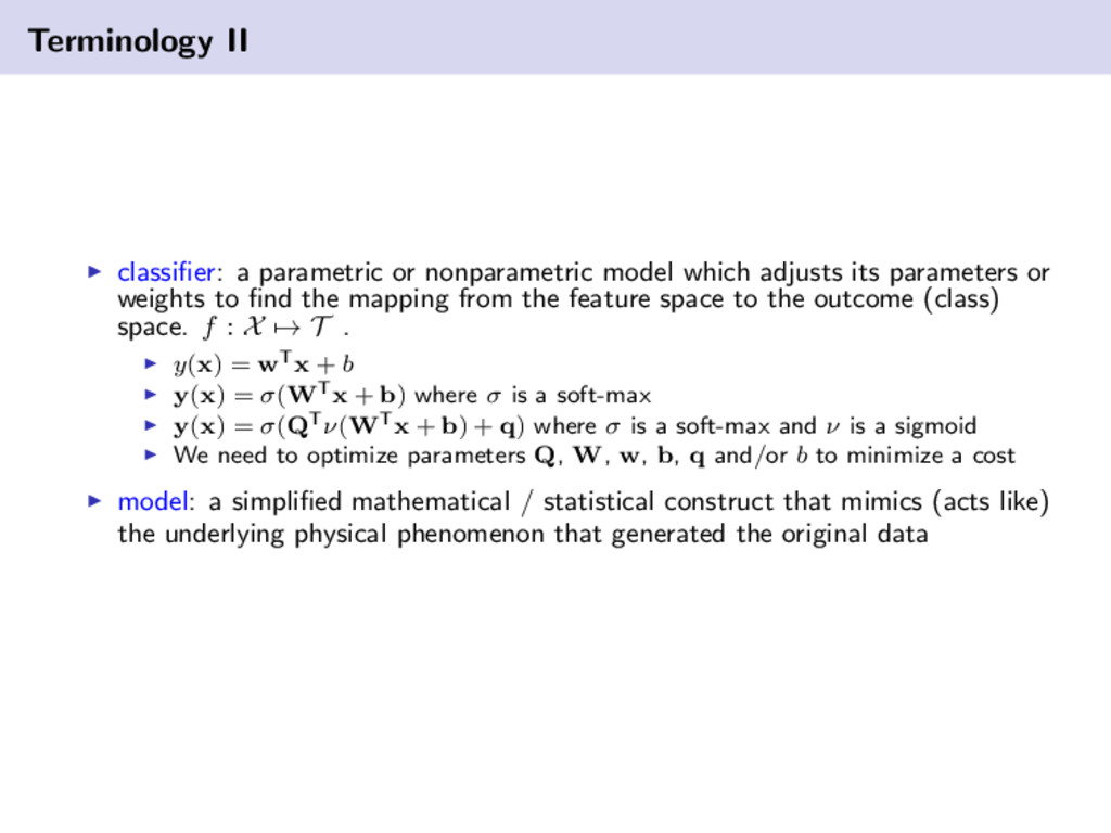
its parameters or weights to find the mapping from the feature space to the outcome (class) space. f : X → T . y(x) = wTx + b y(x) = σ(WTx + b) where σ is a soft-max y(x) = σ(QTν(WTx + b) + q) where σ is a soft-max and ν is a sigmoid We need to optimize parameters Q, W, w, b, q and/or b to minimize a cost model: a simplified mathematical / statistical construct that mimics (acts like) the underlying physical phenomenon that generated the original data
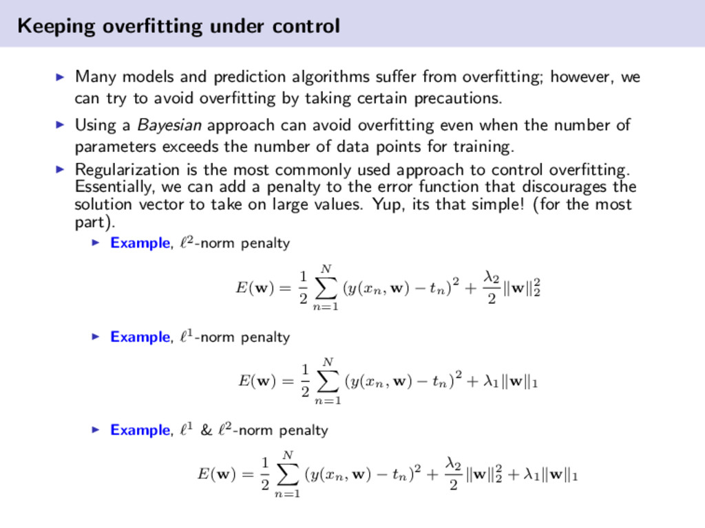
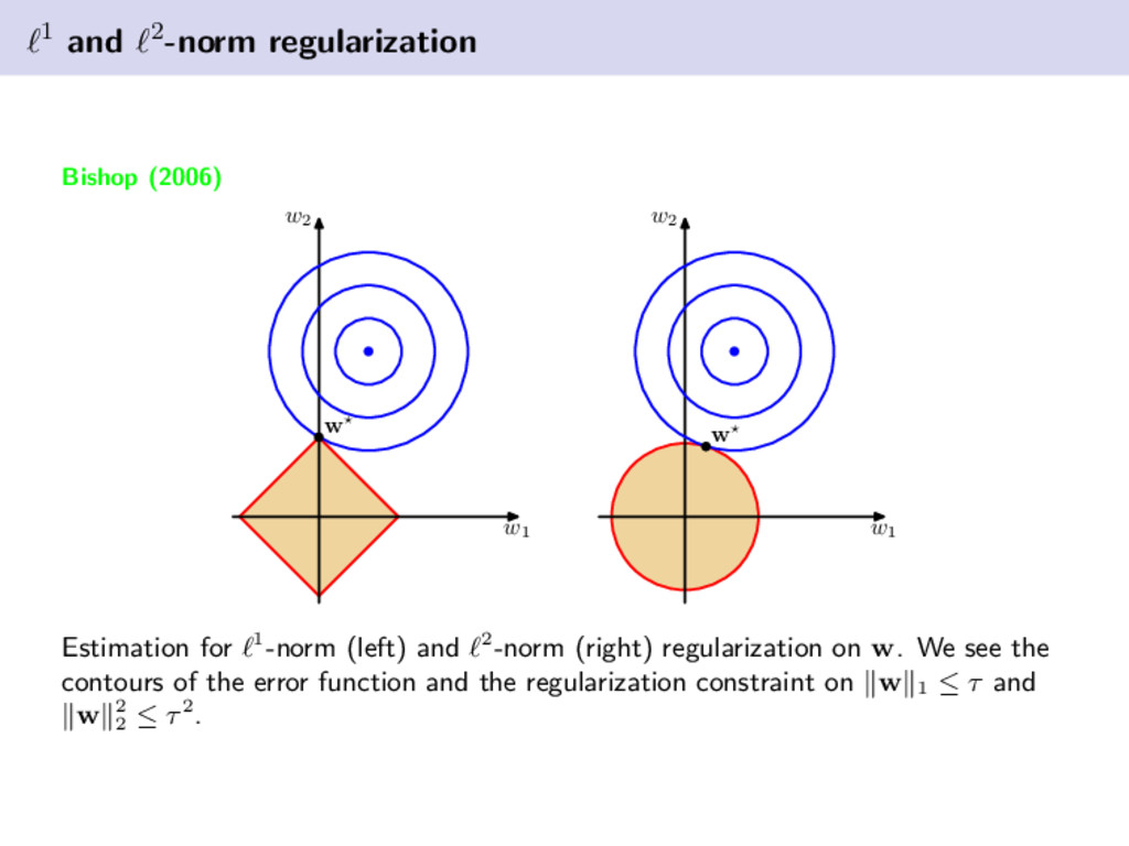
from overfitting; however, we can try to avoid overfitting by taking certain precautions. Using a Bayesian approach can avoid overfitting even when the number of parameters exceeds the number of data points for training. Regularization is the most commonly used approach to control overfitting. Essentially, we can add a penalty to the error function that discourages the solution vector to take on large values. Yup, its that simple! (for the most part). Example, 2-norm penalty E(w) = 1 2 N n=1 (y(xn, w) − tn)2 + λ2 2 w 2 2 Example, 1-norm penalty E(w) = 1 2 N n=1 (y(xn, w) − tn)2 + λ1 w 1 Example, 1 & 2-norm penalty E(w) = 1 2 N n=1 (y(xn, w) − tn)2 + λ2 2 w 2 2 + λ1 w 1
w2 w Estimation for 1-norm (left) and 2-norm (right) regularization on w. We see the contours of the error function and the regularization constraint on w 1 ≤ τ and w 2 2 ≤ τ2.
Bishop (2006) x t N = 15 0 1 −1 0 1 x t N = 100 0 1 −1 0 1 The green line is the target function, the red function is the result of a 9th order polynomial minimizing ERMS , and the blue points are observations sampled from the target function.
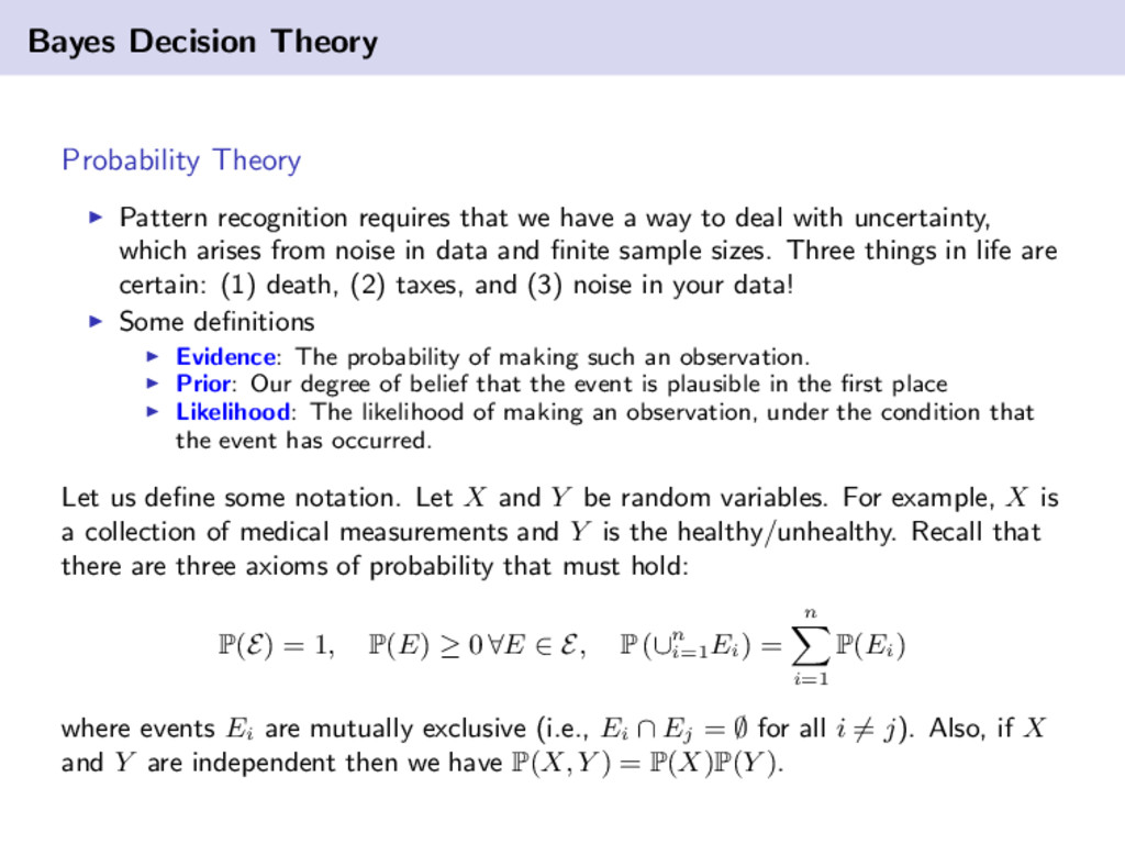
have a way to deal with uncertainty, which arises from noise in data and finite sample sizes. Three things in life are certain: (1) death, (2) taxes, and (3) noise in your data! Some definitions Evidence: The probability of making such an observation. Prior: Our degree of belief that the event is plausible in the first place Likelihood: The likelihood of making an observation, under the condition that the event has occurred. Let us define some notation. Let X and Y be random variables. For example, X is a collection of medical measurements and Y is the healthy/unhealthy. Recall that there are three axioms of probability that must hold: P(E) = 1, P(E) ≥ 0 ∀E ∈ E, P (∪n i=1 Ei ) = n i=1 P(Ei ) where events Ei are mutually exclusive (i.e., Ei ∩ Ej = ∅ for all i = j). Also, if X and Y are independent then we have P(X, Y ) = P(X)P(Y ).
of a single random variable can be computed by integrating (or summing) out the other random variables in the joint distribution. P(X) = Y ∈Y P(X, Y ) Product Rule A joint probability can be written as the product of a conditional and marginal probability. P(X, Y ) = P(Y )P(X|Y ) = P(X)P(Y |X) Bayes Rule A simple manipulation of the product rule gives rise to the Bayes rule. P(Y |X) = P(Y )P(X|Y ) P(X) = P(Y )P(X|Y ) Y ∈Y P(X, Y ) = P(Y )P(X|Y ) Y ∈Y P(Y )P(X|Y )
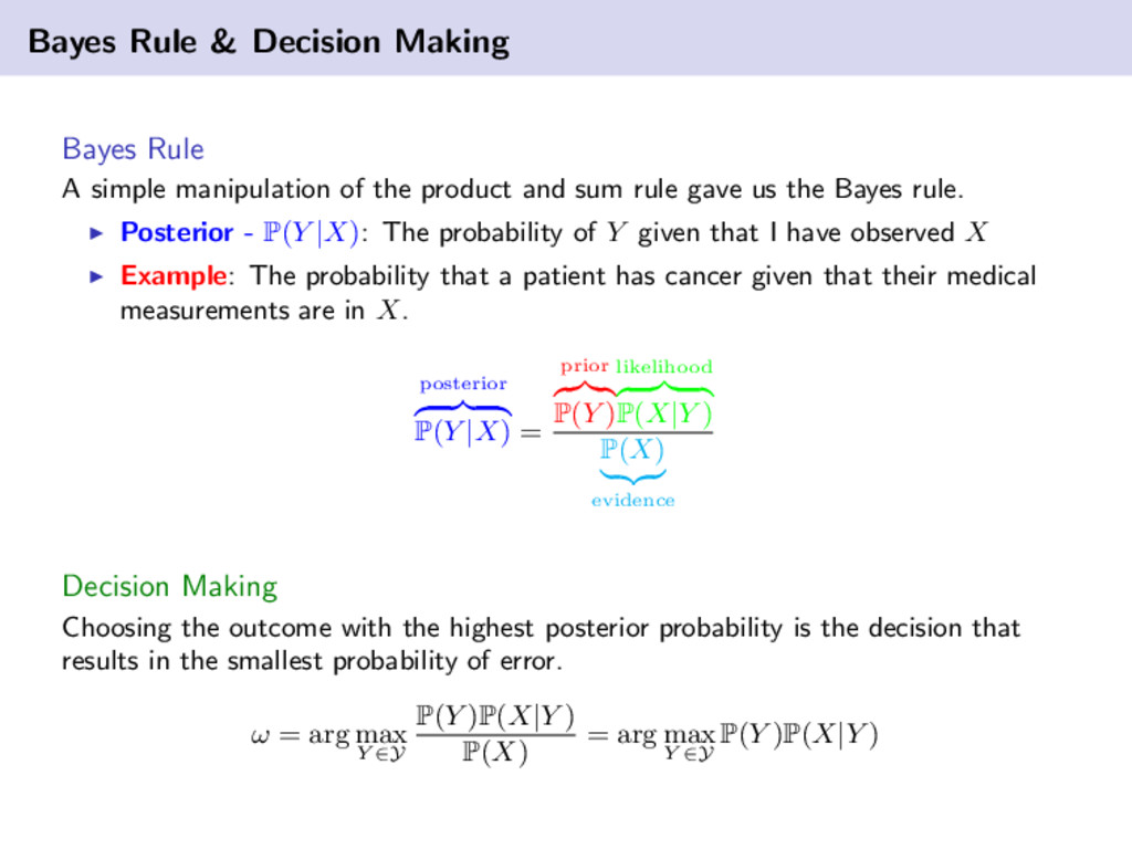
of the product and sum rule gave us the Bayes rule. Posterior - P(Y |X): The probability of Y given that I have observed X Example: The probability that a patient has cancer given that their medical measurements are in X. posterior P(Y |X) = prior P(Y ) likelihood P(X|Y ) P(X) evidence Decision Making Choosing the outcome with the highest posterior probability is the decision that results in the smallest probability of error. ω = arg max Y ∈Y P(Y )P(X|Y ) P(X) = arg max Y ∈Y P(Y )P(X|Y )
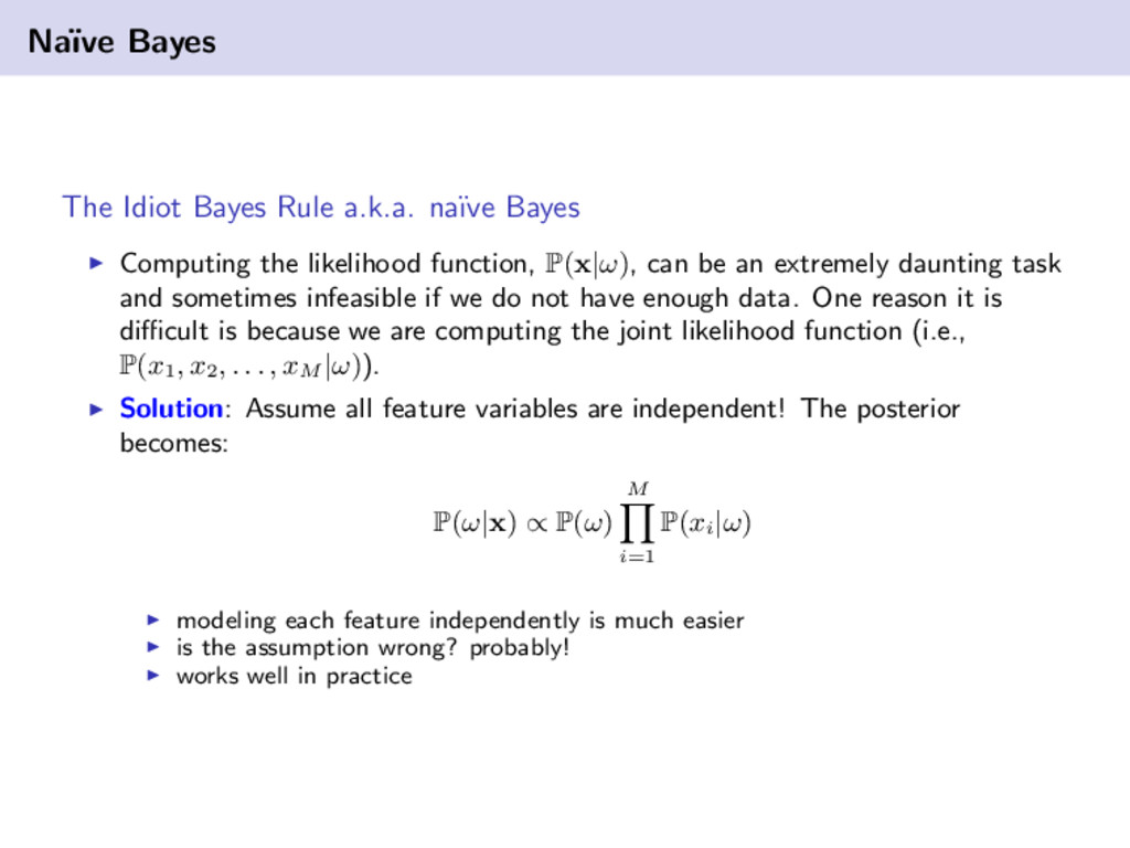
Bayes Computing the likelihood function, P(x|ω), can be an extremely daunting task and sometimes infeasible if we do not have enough data. One reason it is difficult is because we are computing the joint likelihood function (i.e., P(x1 , x2 , . . . , xM |ω)). Solution: Assume all feature variables are independent! The posterior becomes: P(ω|x) ∝ P(ω) M i=1 P(xi |ω) modeling each feature independently is much easier is the assumption wrong? probably! works well in practice
a decision with the smallest probability of error! So does that mean we are done? Some things to think about What if we do not know the form of P(X|Y )? What if we incorrectly assume the form of the distribution? What if we have a small sample size? Can we be confident in P(Y )? More features generally means we need more data to “accurately” estimate any of the models parameters.
(Breiman et al., 1984), and C4.5 (Quinlan, 1986) are two of the more popular methods for generating decision trees. Decision trees provide a natural setting to handle data for containing categorical variables, but can still use continuous variables. Pros & Cons Decision trees are unstable classifiers – a small change on the input can produce a large change on the output. con Prone to overfitting. con Easy to interpret! pro
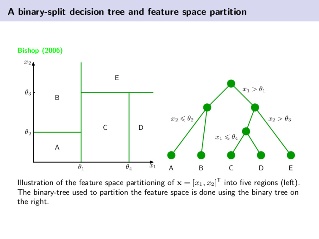
A B C D E θ1 θ4 θ2 θ3 x1 x2 x1 > θ1 x2 > θ3 x1 θ4 x2 θ2 A B C D E Illustration of the feature space partitioning of x = [x1 , x2 ]T into five regions (left). The binary-tree used to partition the feature space is done using the binary tree on the right.
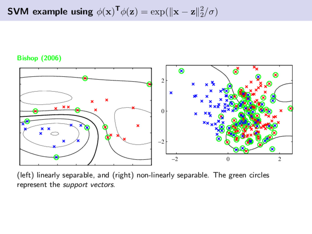
classification models that maximize the margin between the two-classes. The determination of an SVM model is found via a convex optimization problem. Kernel methods can be used to solve non-linear problems with the SVM. The output of the SVM given by y(x) = wTφ(x) + b, where φ(·) is a non-linear feature transform. Overview Support vector machines are binary classification models that maximize the margin between two classes. Let tn ∈ {±1}. The determination of the solution parameters to the SVM is found via a convex optimization problem. For a convex function, if we have a local solution then it is a global solution.
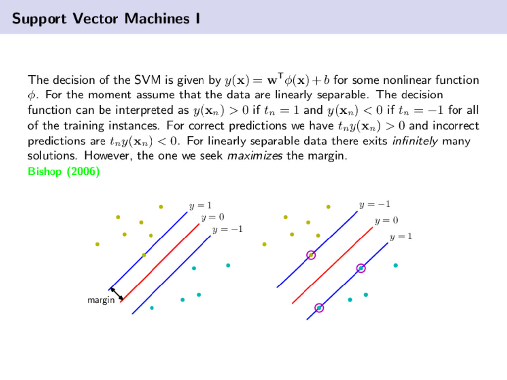
given by y(x) = wTφ(x) + b for some nonlinear function φ. For the moment assume that the data are linearly separable. The decision function can be interpreted as y(xn ) > 0 if tn = 1 and y(xn ) < 0 if tn = −1 for all of the training instances. For correct predictions we have tn y(xn ) > 0 and incorrect predictions are tn y(xn ) < 0. For linearly separable data there exits infinitely many solutions. However, the one we seek maximizes the margin. Bishop (2006) y = 1 y = 0 y = −1 margin y = 1 y = 0 y = −1
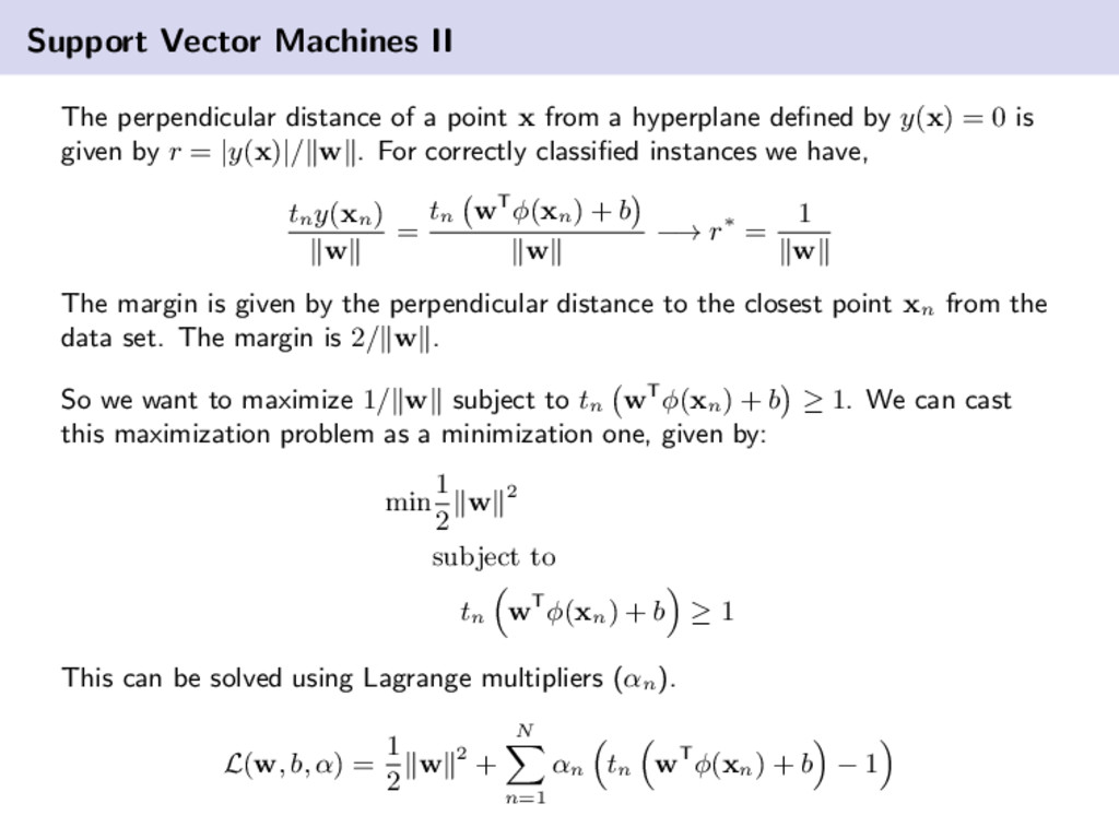
x from a hyperplane defined by y(x) = 0 is given by r = |y(x)|/ w . For correctly classified instances we have, tn y(xn ) w = tn wTφ(xn ) + b w −→ r∗ = 1 w The margin is given by the perpendicular distance to the closest point xn from the data set. The margin is 2/ w . So we want to maximize 1/ w subject to tn wTφ(xn ) + b ≥ 1. We can cast this maximization problem as a minimization one, given by: min 1 2 w 2 subject to tn wTφ(xn ) + b ≥ 1 This can be solved using Lagrange multipliers (αn ). L(w, b, α) = 1 2 w 2 + N n=1 αn tn wTφ(xn ) + b − 1
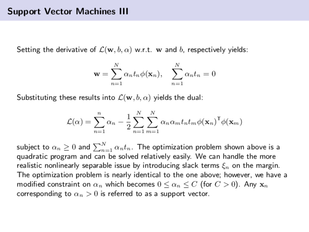
α) w.r.t. w and b, respectively yields: w = N n=1 αn tn φ(xn ), N n=1 αn tn = 0 Substituting these results into L(w, b, α) yields the dual: L(α) = n n=1 αn − 1 2 N n=1 N m=1 αn αm tn tm φ(xn )Tφ(xm ) subject to αn ≥ 0 and N n=1 αn tn . The optimization problem shown above is a quadratic program and can be solved relatively easily. We can handle the more realistic nonlinearly separable issue by introducing slack terms ξn on the margin. The optimization problem is nearly identical to the one above; however, we have a modified constraint on αn which becomes 0 ≤ αn ≤ C (for C > 0). Any xn corresponding to αn > 0 is referred to as a support vector.
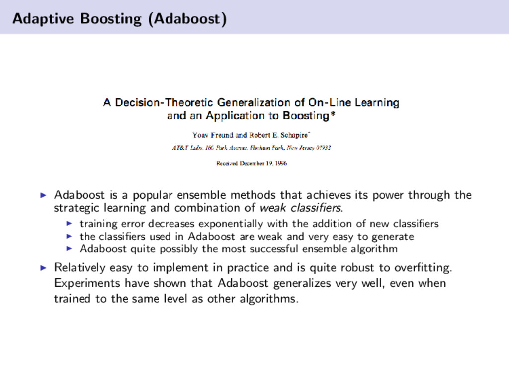
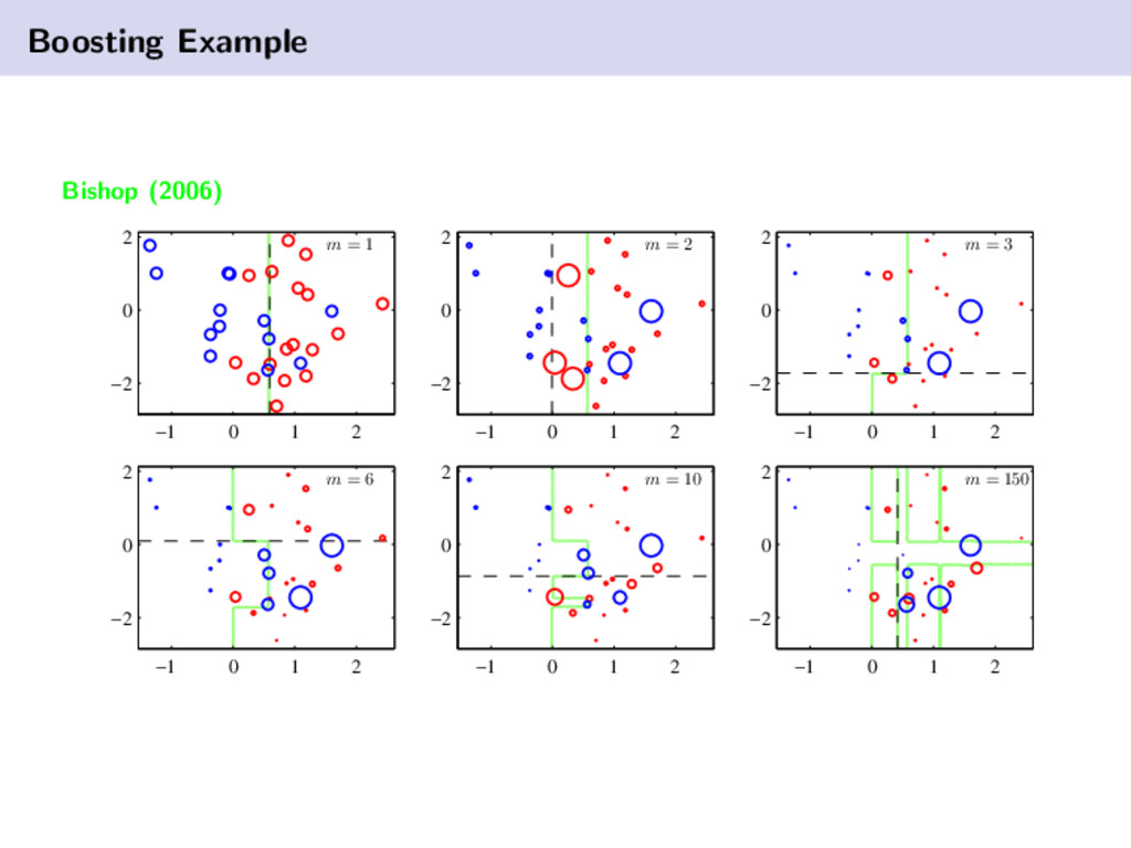
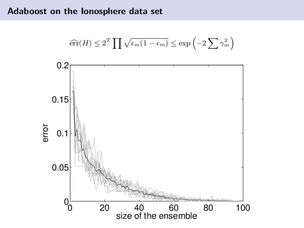
achieves its power through the strategic learning and combination of weak classifiers. training error decreases exponentially with the addition of new classifiers the classifiers used in Adaboost are weak and very easy to generate Adaboost quite possibly the most successful ensemble algorithm Relatively easy to implement in practice and is quite robust to overfitting. Experiments have shown that Adaboost generalizes very well, even when trained to the same level as other algorithms.
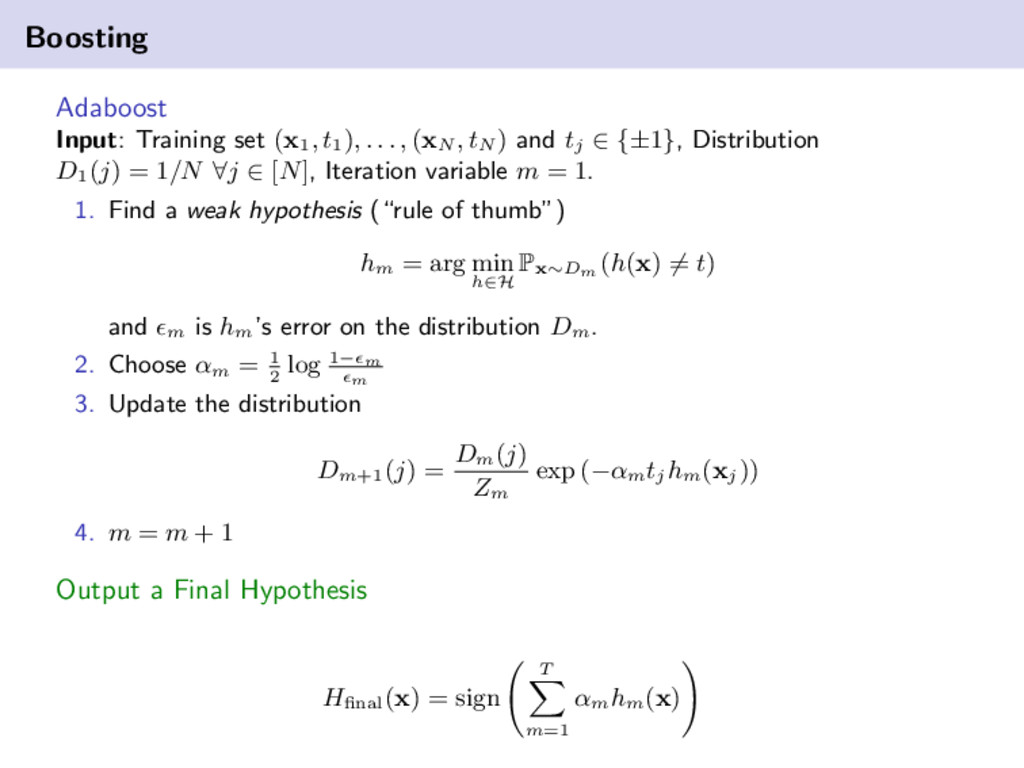
. . , (xN , tN ) and tj ∈ {±1}, Distribution D1 (j) = 1/N ∀j ∈ [N], Iteration variable m = 1. 1. Find a weak hypothesis (“rule of thumb”) hm = arg min h∈H Px∼Dm (h(x) = t) and m is hm ’s error on the distribution Dm . 2. Choose αm = 1 2 log 1− m m 3. Update the distribution Dm+1 (j) = Dm (j) Zm exp (−αm tj hm (xj )) 4. m = m + 1 Output a Final Hypothesis Hfinal (x) = sign T m=1 αm hm (x)