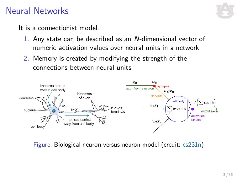
can be described as an N-dimensional vector of numeric activation values over neural units in a network. 2. Memory is created by modifying the strength of the connections between neural units. Figure: Biological neuron versus neuron model (credit: cs231n) 3 / 35
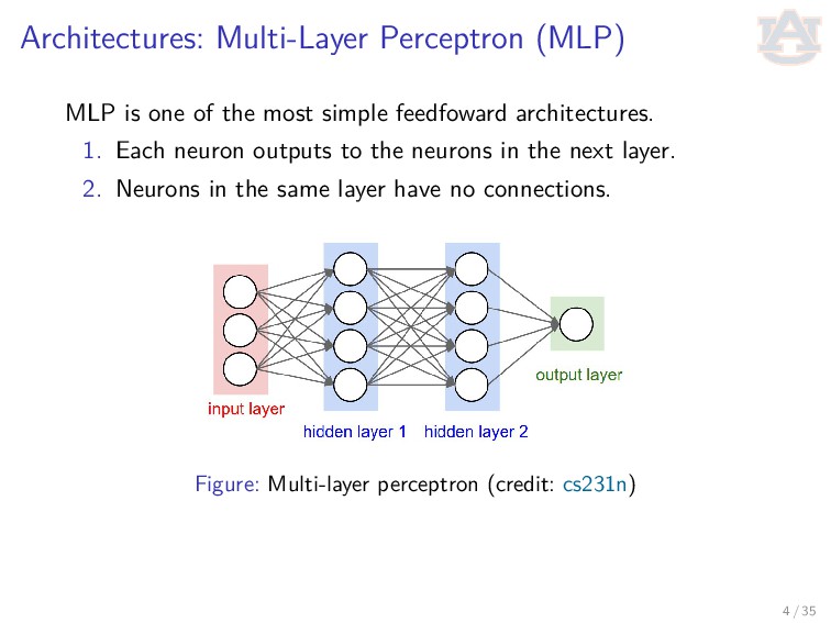
simple feedfoward architectures. 1. Each neuron outputs to the neurons in the next layer. 2. Neurons in the same layer have no connections. Figure: Multi-layer perceptron (credit: cs231n) 4 / 35
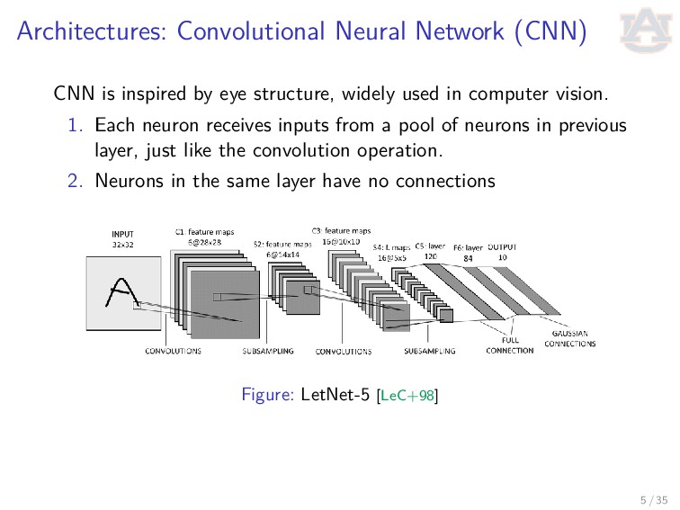
structure, widely used in computer vision. 1. Each neuron receives inputs from a pool of neurons in previous layer, just like the convolution operation. 2. Neurons in the same layer have no connections Figure: LetNet-5 [LeC+98] 5 / 35
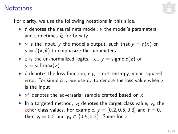
slide. f denotes the neural nets model, θ the model’s parameters, and sometimes fθ for brevity. x is the input, y the model’s output, such that y = f (x) or y = f (x; θ) to emphasize the parameters. z is the un-normalized logits, i.e., y = sigmoid(z) or y = softmax(z). L denotes the loss function, e.g., cross-entropy, mean-squared error. For simplicity, we use Lx to denote the loss value when x is the input. x∗ denotes the adversarial sample crafted based on x. In a targeted method, yt denotes the target class value, yo the other class values. For example, y = [0.2, 0.5, 0.3] and t = 0, then yt = 0.2 and yo ∈ {0.5, 0.3}. Same for z. 7 / 35
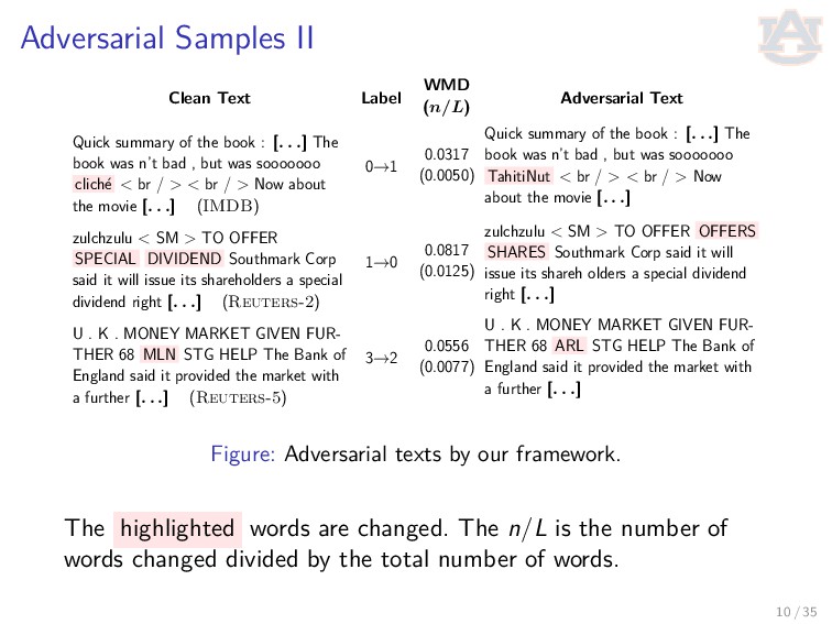
Quick summary of the book : [. . .] The book was n’t bad , but was sooooooo clich´ e < br / > < br / > Now about the movie [. . .] (IMDB) 0→1 0.0317 (0.0050) Quick summary of the book : [. . .] The book was n’t bad , but was sooooooo TahitiNut < br / > < br / > Now about the movie [. . .] zulchzulu < SM > TO OFFER SPECIAL DIVIDEND Southmark Corp said it will issue its shareholders a special dividend right [. . .] (Reuters-2) 1→0 0.0817 (0.0125) zulchzulu < SM > TO OFFER OFFERS SHARES Southmark Corp said it will issue its shareh olders a special dividend right [. . .] U . K . MONEY MARKET GIVEN FUR- THER 68 MLN STG HELP The Bank of England said it provided the market with a further [. . .] (Reuters-5) 3→2 0.0556 (0.0077) U . K . MONEY MARKET GIVEN FUR- THER 68 ARL STG HELP The Bank of England said it provided the market with a further [. . .] Figure: Adversarial texts by our framework. The highlighted words are changed. The n/L is the number of words changed divided by the total number of words. 10 / 35
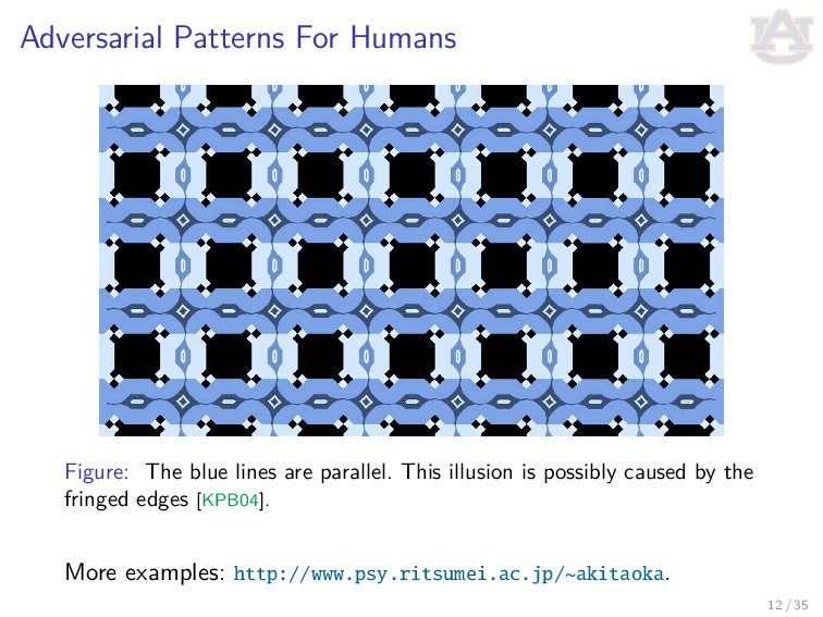
practice and in theory. 1. It undermines the models’ reliability. 2. Hard to ignore due to it being transferable and universal. 3. It provides new insights into neural networks: Local generalization does not seem to hold. Data distribution: they appear in dense regions. Trade-off between robustness and generalization. · · · 13 / 35
points towards the decision boundary [MFF15; Moo+16], in the direction where loss increases for the clean samples [GSS14; KGB16], or decreases for the for the adversarial decreases [Sze+13], or increase the probability for the correct label and/or decrease the others [Pap+15; CW16]. 2. Map between clean and adversarial data points [ZDS17; BF17; Xia+18]. 15 / 35
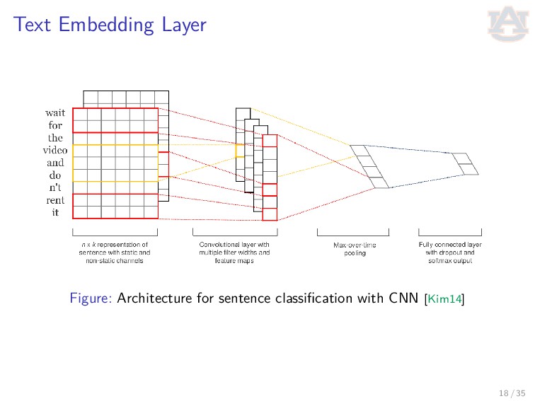
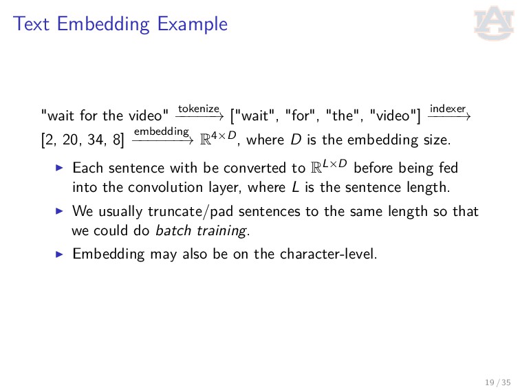
− − − → ["wait", "for", "the", "video"] indexer − − − − → [2, 20, 34, 8] embedding − − − − − − → R4×D, where D is the embedding size. Each sentence with be converted to RL×D before being fed into the convolution layer, where L is the sentence length. We usually truncate/pad sentences to the same length so that we could do batch training. Embedding may also be on the character-level. 19 / 35
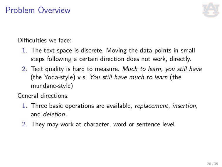
discrete. Moving the data points in small steps following a certain direction does not work, directly. 2. Text quality is hard to measure. Much to learn, you still have (the Yoda-style) v.s. You still have much to learn (the mundane-style) General directions: 1. Three basic operations are available, replacement, insertion, and deletion. 2. They may work at character, word or sentence level. 20 / 35
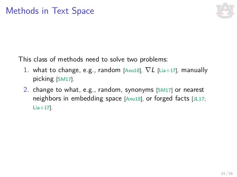
solve two problems: 1. what to change, e.g., random [Ano18], ∇L [Lia+17], manually picking [SM17]. 2. change to what, e.g., random, synonyms [SM17] or nearest neighbors in embedding space [Ano18], or forged facts [JL17; Lia+17]. 21 / 35
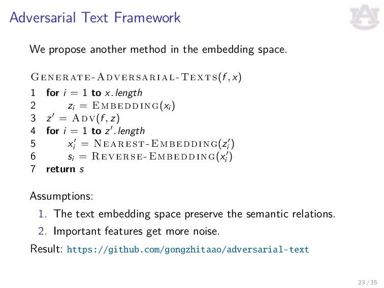
space. Generate-Adversarial-Texts(f , x) 1 for i = 1 to x.length 2 zi = Embedding(xi ) 3 z = Adv(f , z) 4 for i = 1 to z .length 5 xi = Nearest-Embedding(zi ) 6 si = Reverse-Embedding(xi ) 7 return s Assumptions: 1. The text embedding space preserve the semantic relations. 2. Important features get more noise. Result: https://github.com/gongzhitaao/adversarial-text 23 / 35
language model scores, Word Mover’s Distance (WMD). 2. Find a way to control the quality of generated adversarial texts. 3. Test the transferability of adversarial texts. 24 / 35
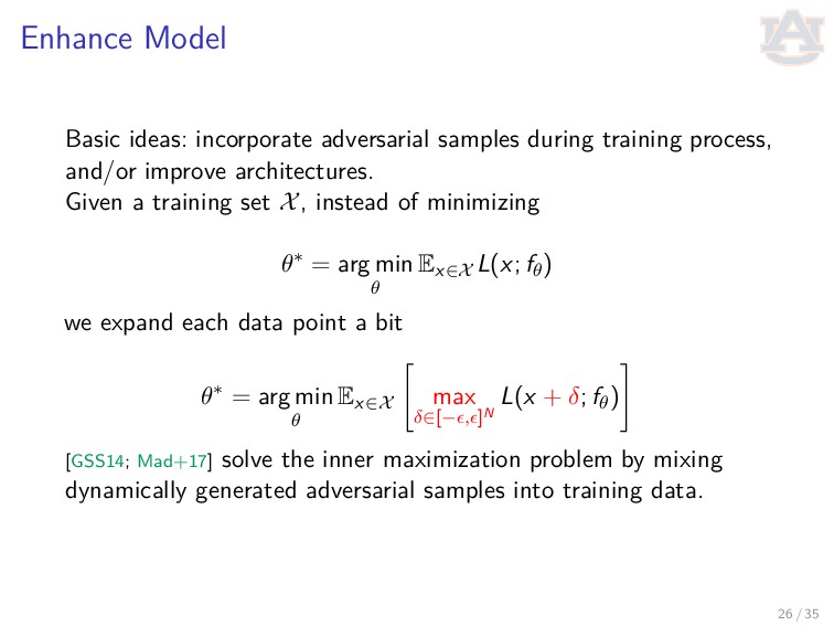
and/or improve architectures. Given a training set X, instead of minimizing θ∗ = arg min θ Ex∈X L(x; fθ) we expand each data point a bit θ∗ = arg min θ Ex∈X max δ∈[− , ]N L(x + δ; fθ) [GSS14; Mad+17] solve the inner maximization problem by mixing dynamically generated adversarial samples into training data. 26 / 35
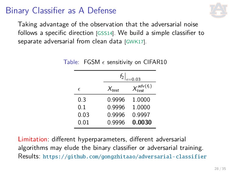
that the adversarial noise follows a specific direction [GSS14]. We build a simple classifier to separate adversarial from clean data [GWK17]. Table: FGSM sensitivity on CIFAR10 f2 =0.03 Xtest Xadv(f1) test 0.3 0.9996 1.0000 0.1 0.9996 1.0000 0.03 0.9996 0.9997 0.01 0.9996 0.0030 Limitation: different hyperparameters, different adversarial algorithms may elude the binary classifier or adversarial training. Results: https://github.com/gongzhitaao/adversarial-classifier 28 / 35
to exist in dense regions. 3. Distribute along only certain directions. 4. Transfer to different models or techniques. 5. · · · ALL EMPIRICAL AND HYPOTHESIS SO FAR 32 / 35
International Conference on Learning Representations (2018). url: https://openreview.net/forum?id=r1QZ3zbAZ. [BF17] Shumeet Baluja and Ian Fischer. “Adversarial Transformation Networks: Learning To Generate Adversarial Examples”. In: CoRR abs/1703.09387 (2017). url: http://arxiv.org/abs/17 3. 9387. [CW16] Nicholas Carlini and David Wagner. “Towards Evaluating the Robustness of Neural Networks”. In: CoRR abs/1608.04644 (2016). url: http://arxiv.org/abs/16 8. 4644. [GSS14] I. J. Goodfellow, J. Shlens, and C. Szegedy. “Explaining and Harnessing Adversarial Examples”. In: ArXiv e-prints (Dec. 2014). arXiv: 1412.6572 [stat.ML]. [GWK17] Zhitao Gong, Wenlu Wang, and Wei-Shinn Ku. “Adversarial and Clean Data Are Not Twins”. In: CoRR abs/1704.04960 (2017). [HS06] G. E. Hinton and R. R. Salakhutdinov. “Reducing the Dimensionality of Data With Neural Networks”. In: Science 313.5786 (2006), pp. 504–507. doi: 1 .1126/science.1127647. eprint: http://www.sciencemag.org/content/313/5786/5 4.full.pdf. url: http://www.sciencemag.org/content/313/5786/5 4.abstract. [JL17] Robin Jia and Percy Liang. “Adversarial Examples for Evaluating Reading Comprehension Systems”. In: arXiv preprint arXiv:1707.07328 (2017). [KGB16] A. Kurakin, I. Goodfellow, and S. Bengio. “Adversarial Examples in the Physical world”. In: ArXiv e-prints (July 2016). arXiv: 16 7. 2533 [cs.CV]. [Kim14] Yoon Kim. “Convolutional Neural Networks for Sentence Classification”. In: CoRR abs/1408.5882 (2014). [KPB04] Akiyoshi Kitaoka, Baingio Pinna, and Gavin Brelstaff. “Contrast Polarities Determine the Direction of Café Wall Tilts”. In: Perception 33.1 (2004), pp. 11–20. [LeC+98] Yann LeCun et al. “Gradient-Based Learning Applied To Document Recognition”. In: Proceedings of the IEEE 86.11 (1998), pp. 2278–2324. [Lia+17] Bin Liang et al. “Deep Text Classification Can Be Fooled”. In: arXiv preprint arXiv:1704.08006 (2017). 34 / 35
![Intuition Figure: Data space hypothesis [NYC14] 16 / 35](https://files.speakerdeck.com/presentations/a1236e8461b345bdb4b0f42d8e43bea0/slide_16.jpg)
![Methods in Transformed Space Autoencoder [HS06] is used to map](https://files.speakerdeck.com/presentations/a1236e8461b345bdb4b0f42d8e43bea0/slide_22.jpg)
![[Ano18] Anonymous. “Adversarial Examples for Natural Language Classification Problems”. In:](https://files.speakerdeck.com/presentations/a1236e8461b345bdb4b0f42d8e43bea0/slide_34.jpg)
![[Mad+17] Aleksander Madry et al. “Towards Deep Learning Models Resistant](https://files.speakerdeck.com/presentations/a1236e8461b345bdb4b0f42d8e43bea0/slide_35.jpg)