A Layered Architecture for EV Charging Stations Based on Time Scale Decomposition

Ke Ma (TAMU), Grid-X Program Presentation on Day 1 (Nov.3) of Workshop on Architecture and Economics of the Future Grid

Transcript

1. 1/21 A Layered Architecture for EV Charging Stations Based on Time Scale Decomposition Ke Ma, Le Xie and P. R. Kumar Dept. of Electrical and Computer Engineering Texas A&M University Email: ke.ma@tamu.edu
2. 2/21 The charging station  Structure Battery Grid Renewable EV chargers
3. 3/21 Grid  Motivation • Guaranteed power supply • Stable (always available)  Complexities • Peak power constraint • Variability of grid power price 0.00 5.00 10.00 15.00 20.00 25.00 30.00 1 11 21 31 41 51 61 71 81 91 Grid power price ($/MWh) January 1, 2012 HB_HOUSTON 0:00 to 24:00 (15 minutes)
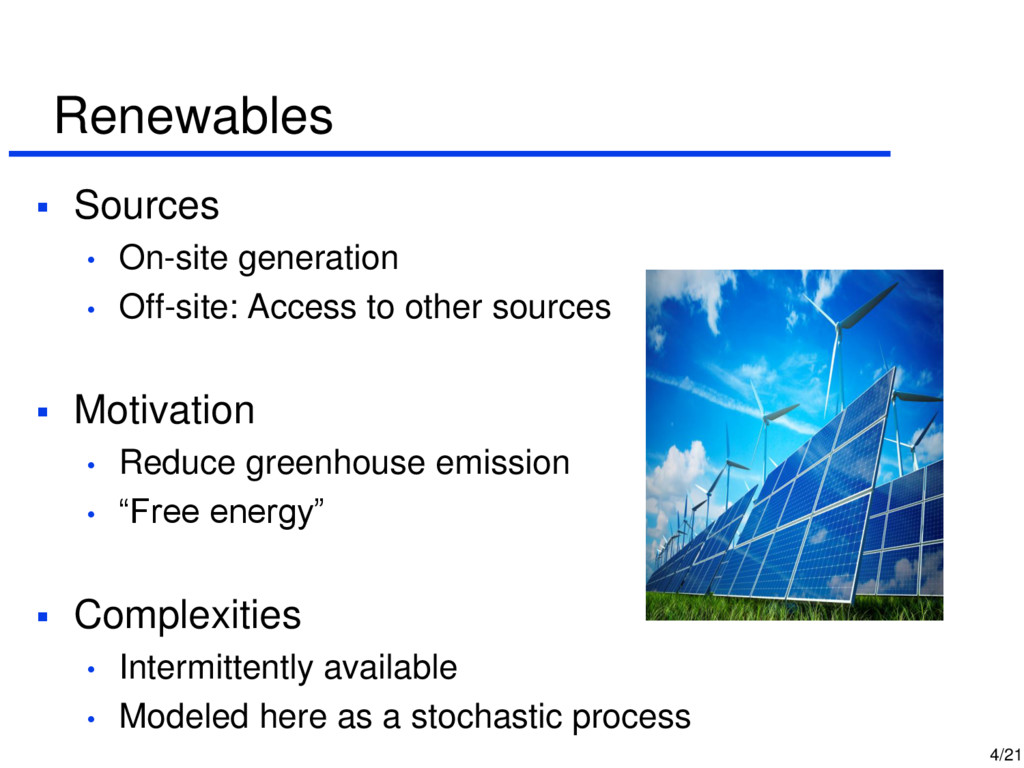
4. 4/21 Renewables  Sources • On-site generation • Off-site: Access to other sources  Motivation • Reduce greenhouse emission • “Free energy”  Complexities • Intermittently available • Modeled here as a stochastic process
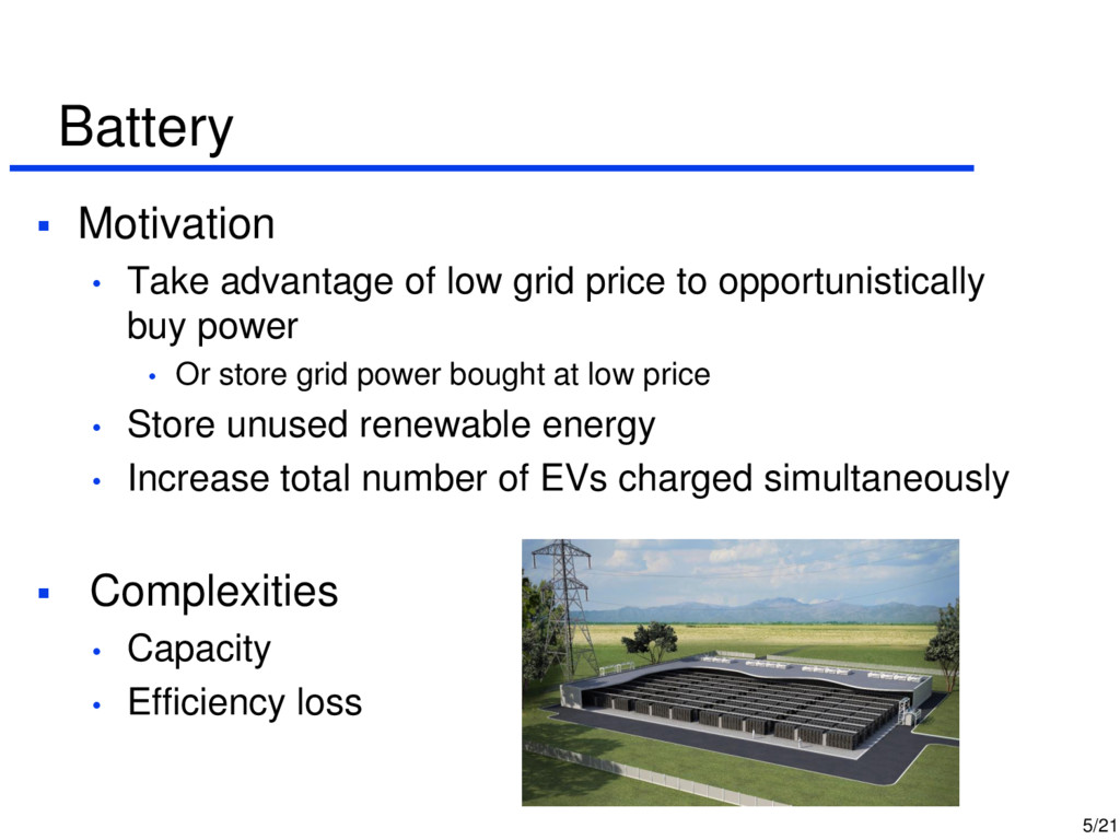
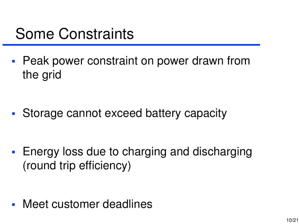
5. 5/21 Battery  Motivation • Take advantage of low grid price to opportunistically buy power • Or store grid power bought at low price • Store unused renewable energy • Increase total number of EVs charged simultaneously  Complexities • Capacity • Efficiency loss
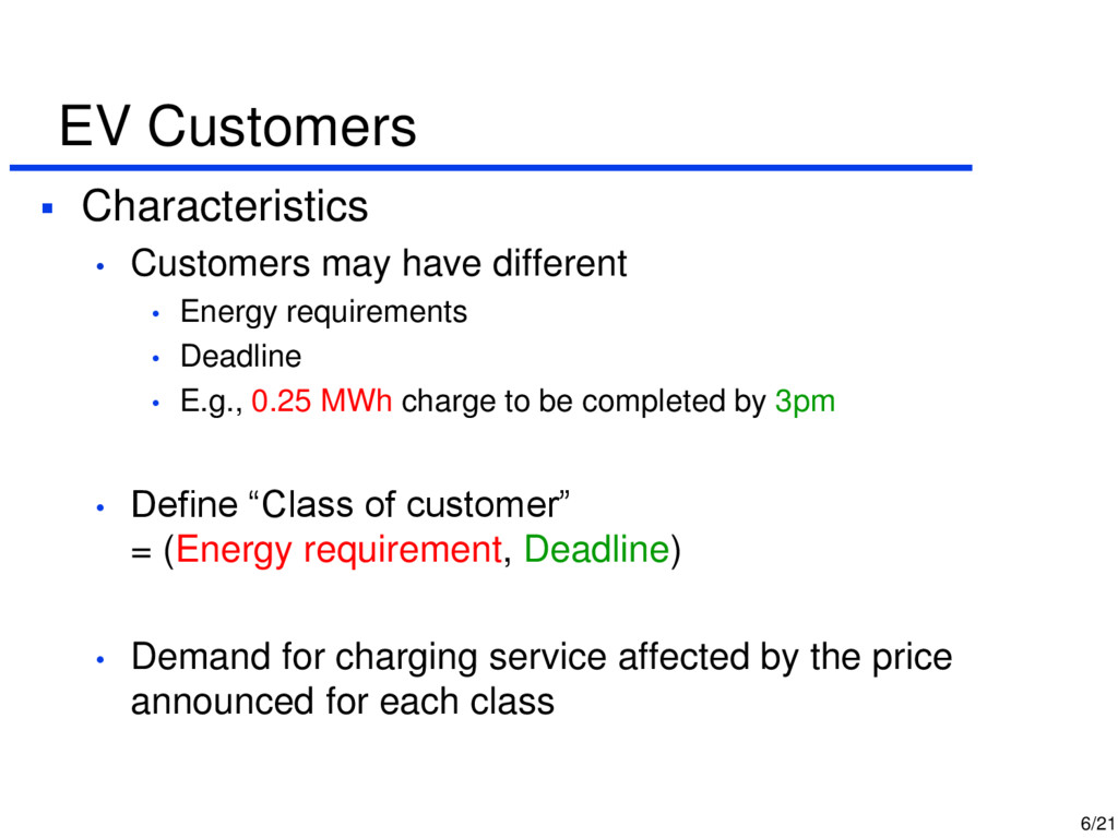
6. 6/21 EV Customers  Characteristics • Customers may have different • Energy requirements • Deadline • E.g., 0.25 MWh charge to be completed by 3pm • Define “Class of customer” = (Energy requirement, Deadline) • Demand for charging service affected by the price announced for each class
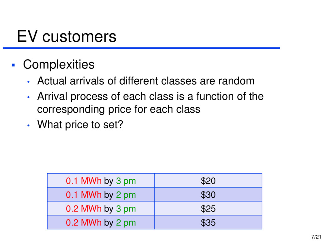
7. 7/21 EV customers  Complexities • Actual arrivals of different classes are random • Arrival process of each class is a function of the corresponding price for each class • What price to set? 0.1 MWh by 3 pm $20 0.1 MWh by 2 pm $30 0.2 MWh by 3 pm $25 0.2 MWh by 2 pm $35
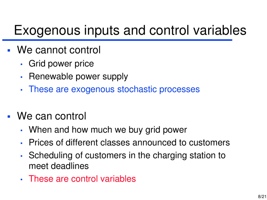
8. 8/21 Exogenous inputs and control variables  We cannot control • Grid power price • Renewable power supply • These are exogenous stochastic processes  We can control • When and how much we buy grid power • Prices of different classes announced to customers • Scheduling of customers in the charging station to meet deadlines • These are control variables
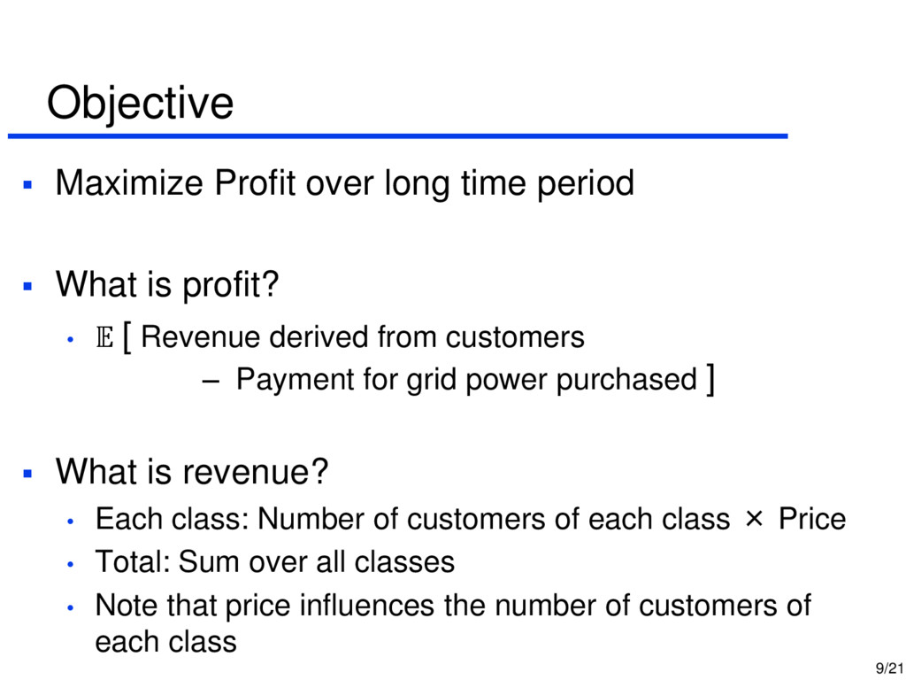
9. 9/21 Objective  Maximize Profit over long time period  What is profit? • [ Revenue derived from customers – Payment for grid power purchased ]  What is revenue? • Each class: Number of customers of each class × Price • Total: Sum over all classes • Note that price influences the number of customers of each class
10. 10/21 Some Constraints  Peak power constraint on power drawn from the grid  Storage cannot exceed battery capacity  Energy loss due to charging and discharging (round trip efficiency)  Meet customer deadlines
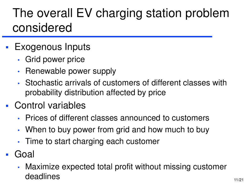
11. 11/21 The overall EV charging station problem considered  Exogenous Inputs • Grid power price • Renewable power supply • Stochastic arrivals of customers of different classes with probability distribution affected by price  Control variables • Prices of different classes announced to customers • When to buy power from grid and how much to buy • Time to start charging each customer  Goal • Maximize expected total profit without missing customer deadlines
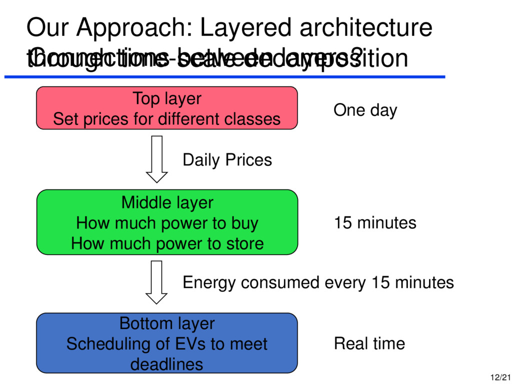
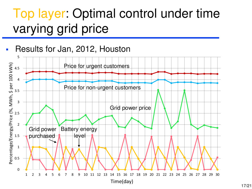
12. 12/21 Our Approach: Layered architecture through time-scale decomposition Daily Prices Energy consumed every 15 minutes One day 15 minutes Real time Top layer Set prices for different classes Middle layer How much power to buy How much power to store Bottom layer Scheduling of EVs to meet deadlines Connections between layers?
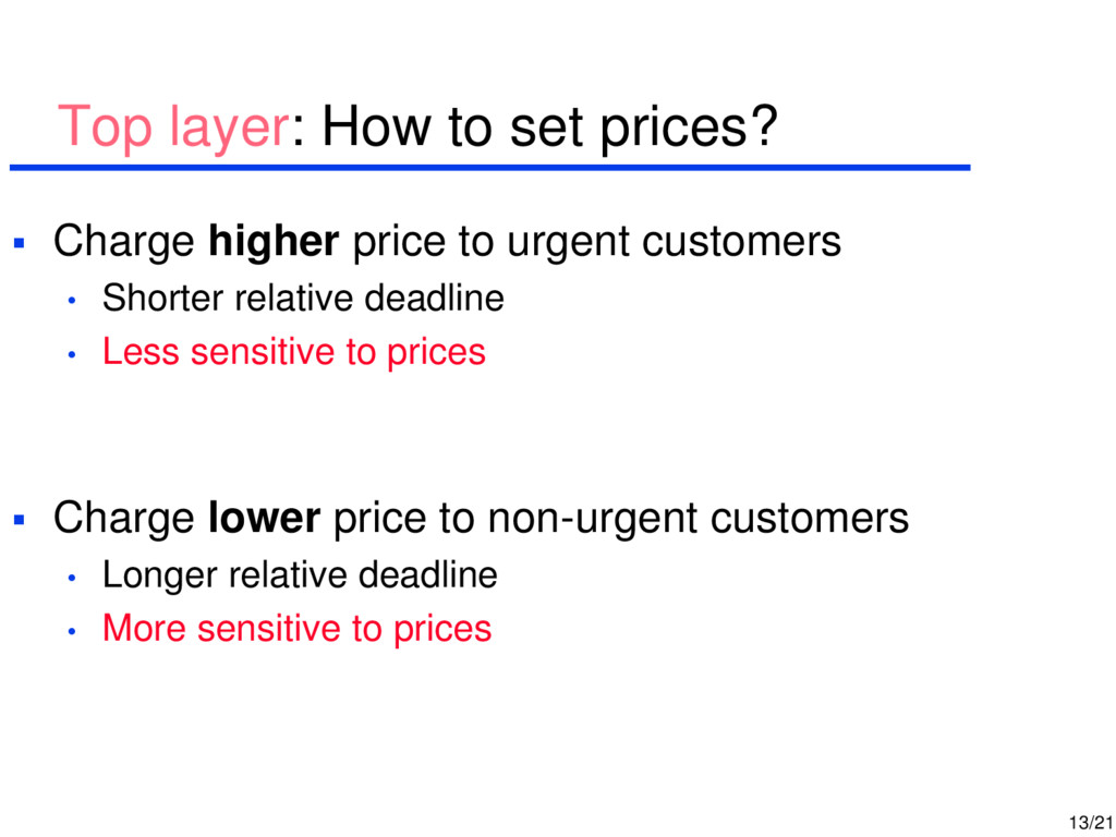
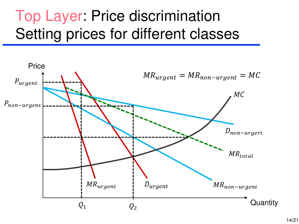
13. 13/21 Top layer: How to set prices?  Charge higher price to urgent customers • Shorter relative deadline • Less sensitive to prices  Charge lower price to non-urgent customers • Longer relative deadline • More sensitive to prices
14. 14/21 Top Layer: Price discrimination Setting prices for different classes Price Quantity − − 1 − 2 = − =
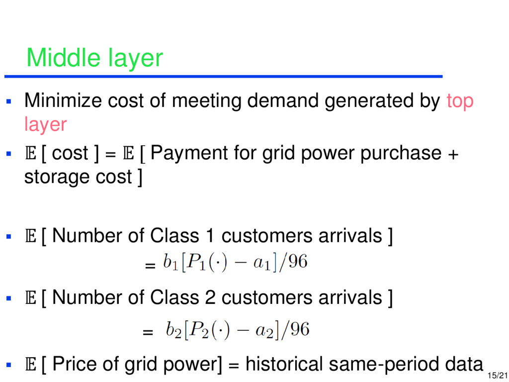
15. 15/21 Middle layer  Minimize cost of meeting demand generated by top layer  [ cost ] = [ Payment for grid power purchase + storage cost ]  [ Number of Class 1 customers arrivals ] =  [ Number of Class 2 customers arrivals ] =  [ Price of grid power] = historical same-period data
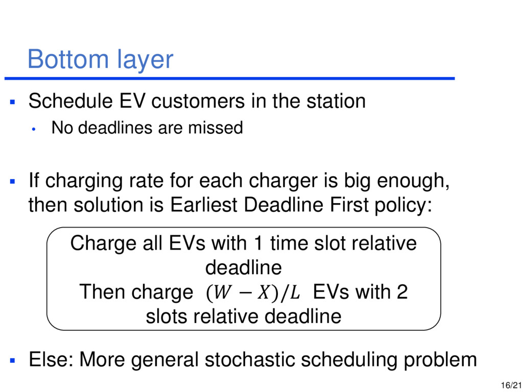
16. 16/21 Bottom layer  Schedule EV customers in the station • No deadlines are missed  If charging rate for each charger is big enough, then solution is Earliest Deadline First policy:  Else: More general stochastic scheduling problem Charge all EVs with 1 time slot relative deadline Then charge ( − )/ EVs with 2 slots relative deadline
17. 17/21 Top layer: Optimal control under time varying grid price  Results for Jan, 2012, Houston 0 0.5 1 1.5 2 2.5 3 3.5 4 4.5 5 1 2 3 4 5 6 7 8 9 10 11 12 13 14 15 16 17 18 19 20 21 22 23 24 25 26 27 28 29 30 Percentage/Energy/Price (%, MWh, $ per 100 kWh) Time(day) Grid power price Price for urgent customers Price for non-urgent customers Grid power purchased Battery energy level
18. 18/21 Computational complexity  Let denote number of customer classes  Top layer • Quadratic programming • 3 + 6 + 5 variables to solve  Middle layer • Discrete time dynamic programming • Sensitive to how finely we discretize the state and action space
19. 19/21 Cost of Layered Policy  Wholesale electricity price from ERCOT (Jan. 1 – 14, 2012)  Upper bound on the profit • Top layer with full future information
20. 20/21 Conclusion  A layered architecture by time scale decomposition  Solve the scheduling, storage and pricing problems  Top layer: planning  Middle layer: adjustment  Bottom layer: real-time scheduling