Wind variability and impact on markets

Prof. Ross Baldick (UT Austin),Presentation on Day 2 (Nov.4) of Workshop on Architecture and Economics of the Future Grid

Transcript

1. 1 Wind variability and impact on markets Workshop on Architecture and Economics of the Future Grid, Texas A&M, November 4, 2016 Duehee Lee, KPMG. Ross Baldick, Department of Electrical and Computer Engineering, University of Texas at Austin.
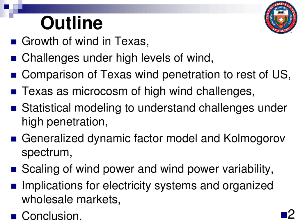
2. Outline  Growth of wind in Texas,  Challenges under high levels of wind,  Comparison of Texas wind penetration to rest of US,  Texas as microcosm of high wind challenges,  Statistical modeling to understand challenges under high penetration,  Generalized dynamic factor model and Kolmogorov spectrum,  Scaling of wind power and wind power variability,  Implications for electricity systems and organized wholesale markets,  Conclusion. 2
3. Texas has experienced remarkable wind growth. 3 0.000 2.000 4.000 6.000 8.000 10.000 12.000 14.000 16.000 18.000 20.000 1999 2000 2001 2002 2003 2004 2005 2006 2007 2008 2009 2010 2011 2012 2013 2014 2015 Wind generation capacity in Texas (GW, end of year) Source: USDOE 2016.
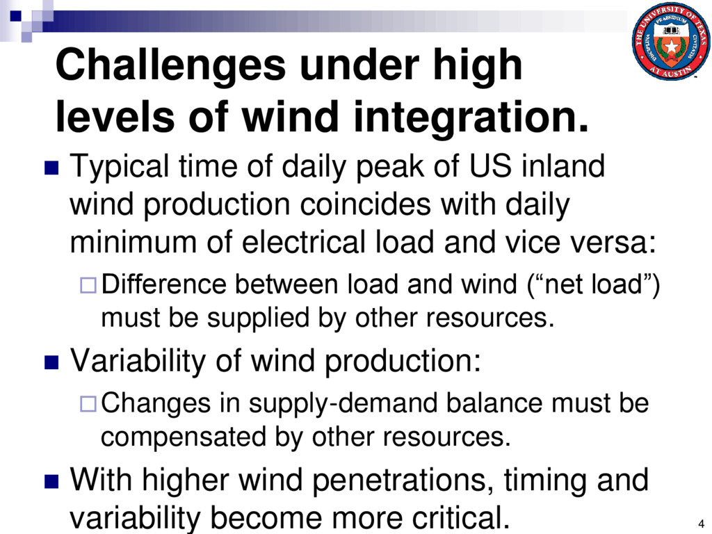
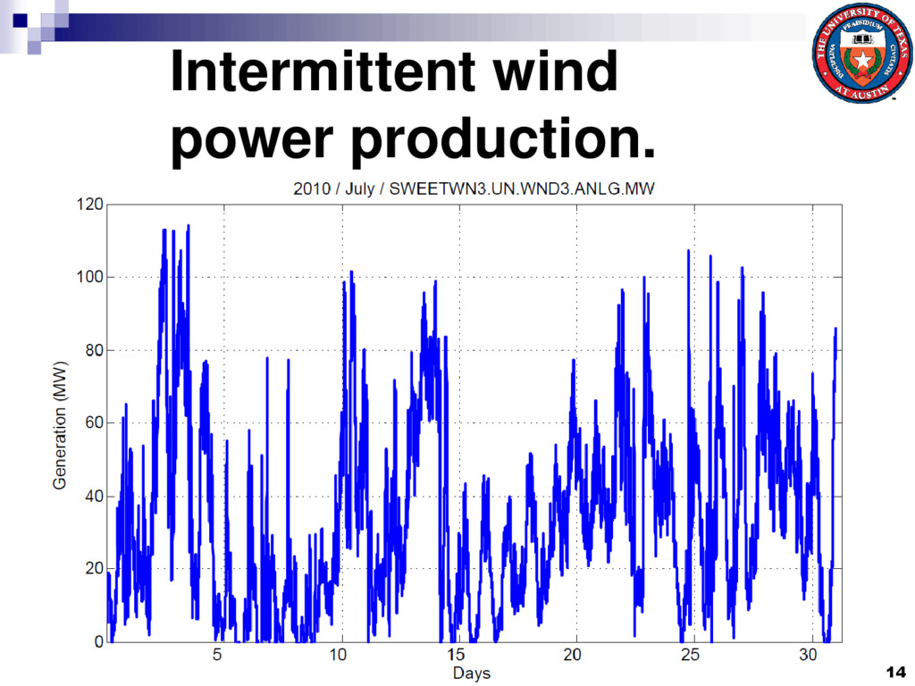
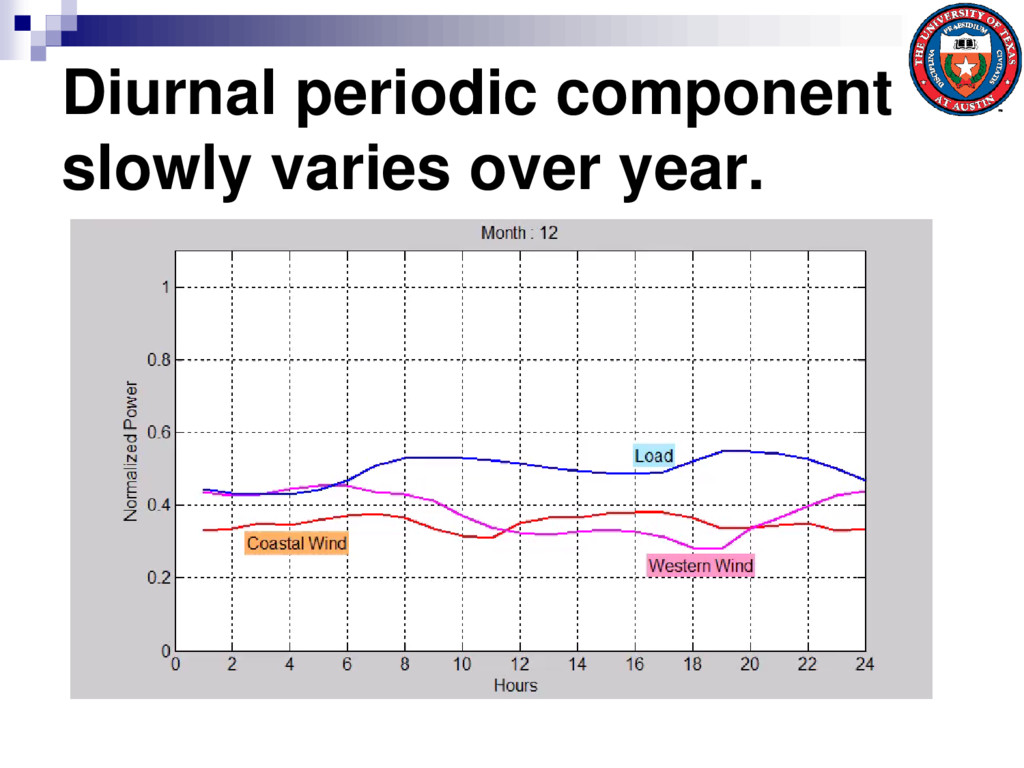
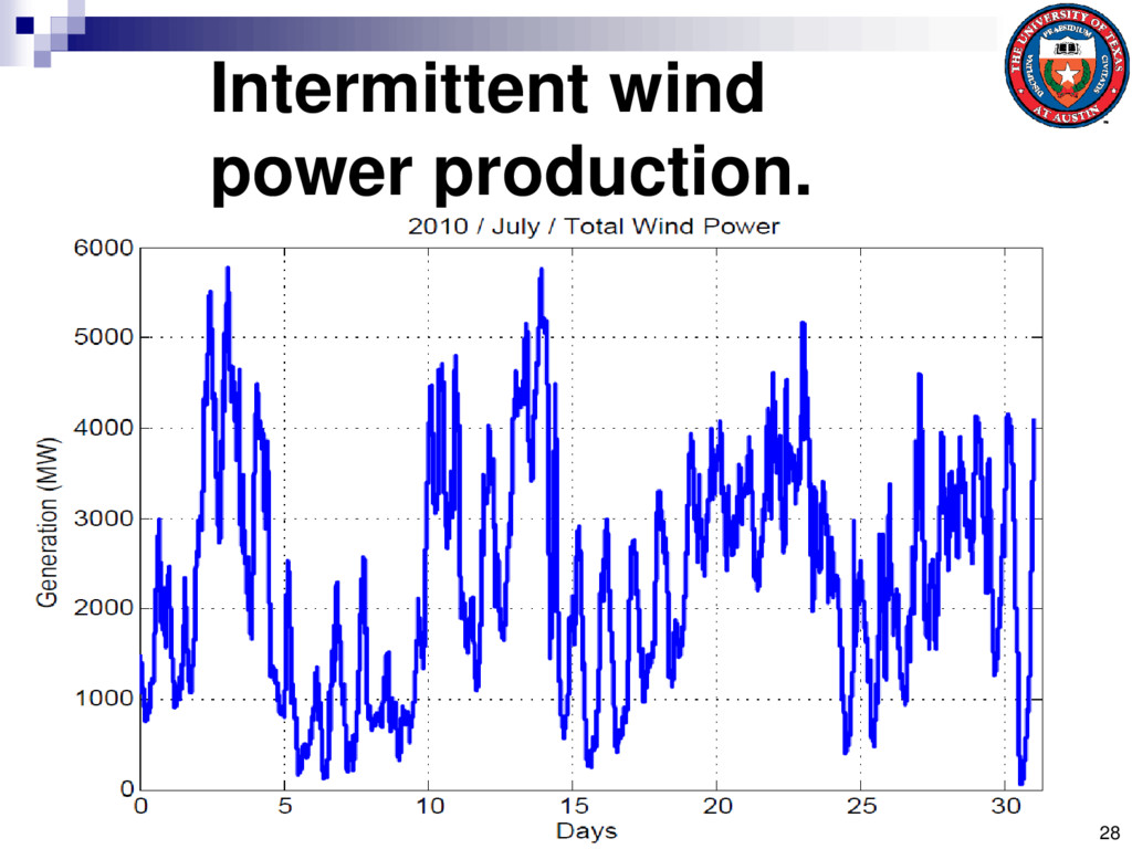
4. Challenges under high levels of wind integration.  Typical time of daily peak of US inland wind production coincides with daily minimum of electrical load and vice versa: Difference between load and wind (“net load”) must be supplied by other resources.  Variability of wind production: Changes in supply-demand balance must be compensated by other resources.  With higher wind penetrations, timing and variability become more critical. 4
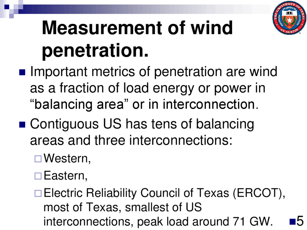
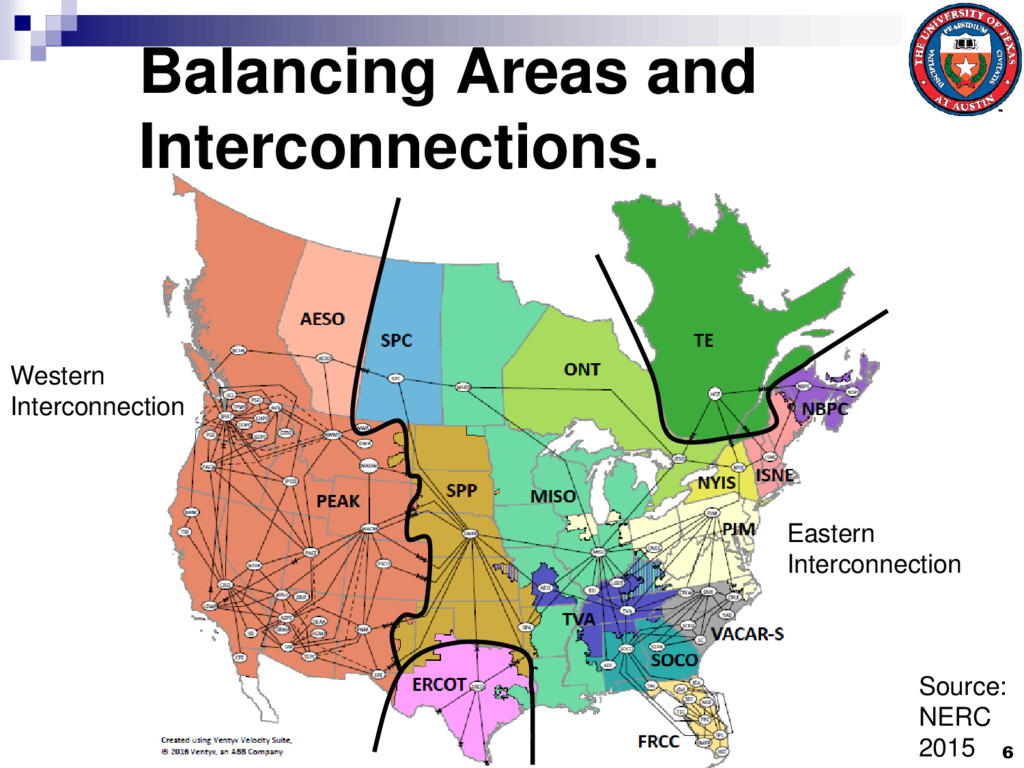
5. Measurement of wind penetration.  Important metrics of penetration are wind as a fraction of load energy or power in “balancing area” or in interconnection.  Contiguous US has tens of balancing areas and three interconnections: Western, Eastern, Electric Reliability Council of Texas (ERCOT), most of Texas, smallest of US interconnections, peak load around 71 GW. 5
6. Balancing Areas and Interconnections. 6 Source: NERC 2015 Western Interconnection Eastern Interconnection
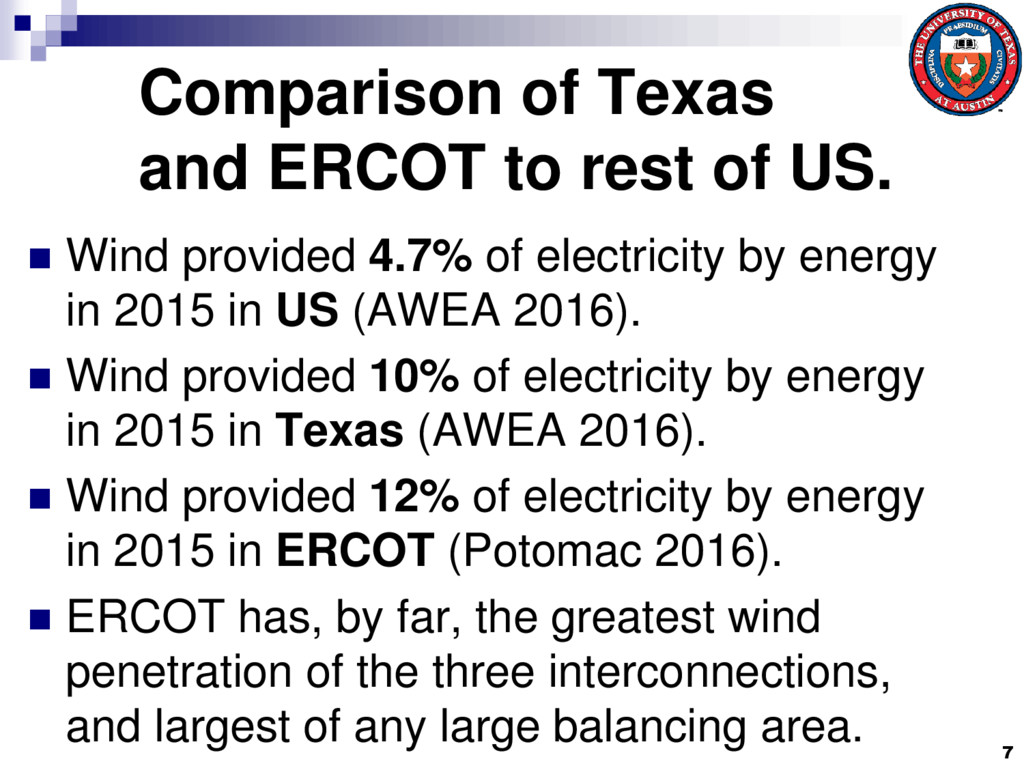
7. Comparison of Texas and ERCOT to rest of US.  Wind provided 4.7% of electricity by energy in 2015 in US (AWEA 2016).  Wind provided 10% of electricity by energy in 2015 in Texas (AWEA 2016).  Wind provided 12% of electricity by energy in 2015 in ERCOT (Potomac 2016).  ERCOT has, by far, the greatest wind penetration of the three interconnections, and largest of any large balancing area. 7
8. 8 West Zone Peak load 5 GW, Generation 16 GW, Wind 12 GW North Zone Peak load 28 GW, Generation 34 GW Wind 1 GW South Zone Peak load 19 GW, Generation 27.5 GW Wind 3 GW Houston Zone Peak load 19 GW, Generation 19 GW Most ERCOT wind is in West Texas zone. Source: Potomac 2016
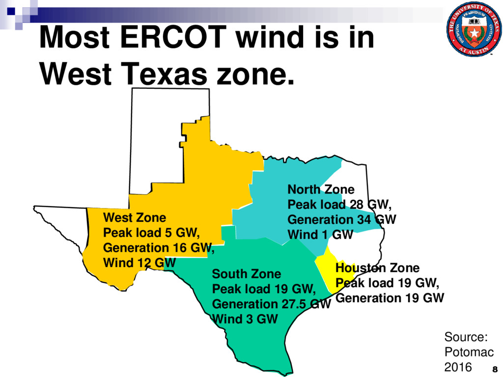
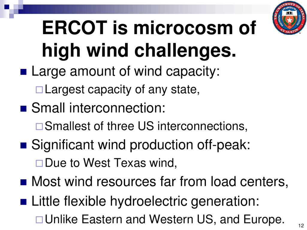
9. ERCOT is microcosm of high wind challenges.  Large amount of wind capacity: Largest capacity of any state,  Small interconnection: Smallest of three US interconnections,  Significant wind production off-peak: Due to West Texas wind,  Most wind resources far from load centers,  Little flexible hydroelectric generation: Unlike Eastern and Western US, and Europe. 12
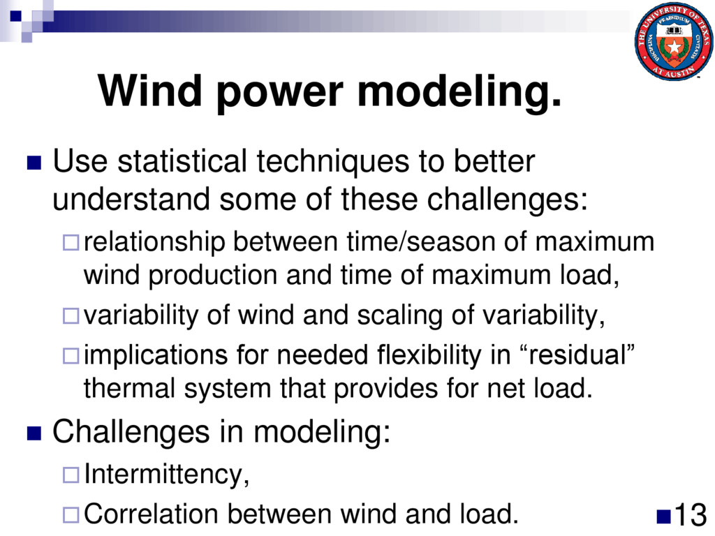
10. Wind power modeling.  Use statistical techniques to better understand some of these challenges: relationship between time/season of maximum wind production and time of maximum load, variability of wind and scaling of variability, implications for needed flexibility in “residual” thermal system that provides for net load.  Challenges in modeling: Intermittency, Correlation between wind and load. 13
11. Intermittent wind power production. 14
12. Correlation of ERCOT wind and load. 15 West Texas wind Load Coastal wind West Texas wind Coastal wind Load
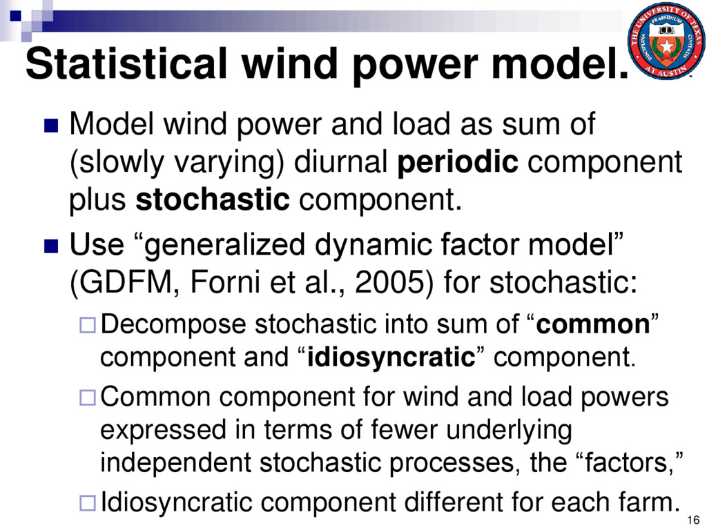
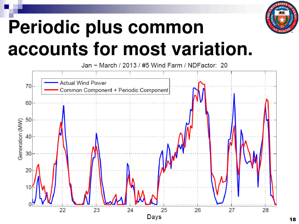
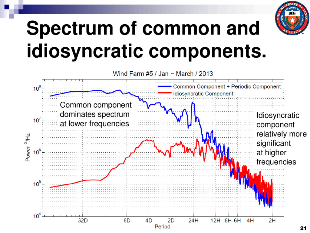
13. Statistical wind power model.  Model wind power and load as sum of (slowly varying) diurnal periodic component plus stochastic component.  Use “generalized dynamic factor model” (GDFM, Forni et al., 2005) for stochastic: Decompose stochastic into sum of “common” component and “idiosyncratic” component. Common component for wind and load powers expressed in terms of fewer underlying independent stochastic processes, the “factors,” Idiosyncratic component different for each farm. 16
14. Diurnal periodic component slowly varies over year.
15. Periodic plus common accounts for most variation. 18
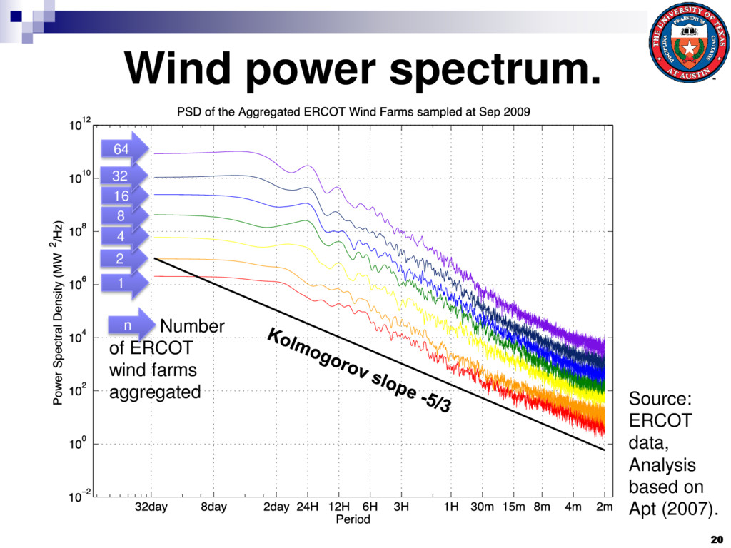
16. Kolmogorov slope of wind power spectrum  A. N. Kolmogorov mainly known to electrical engineers through contributions to understanding of stochastic processes.  Related contributions in turbulent flow recently crossed over to electrical engineering community through Apt (2007).  Kolmogorov used dimension analysis to predict that power spectral density of wind would have characteristic roll-off of slope -5/3.  Verified in Apt (2007). 19
17. 20 1 2 4 8 16 32 64 Number of ERCOT wind farms aggregated Wind power spectrum. Source: ERCOT data, Analysis based on Apt (2007). n
18. Spectrum of common and idiosyncratic components. 21 Common component dominates spectrum at lower frequencies Idiosyncratic component relatively more significant at higher frequencies
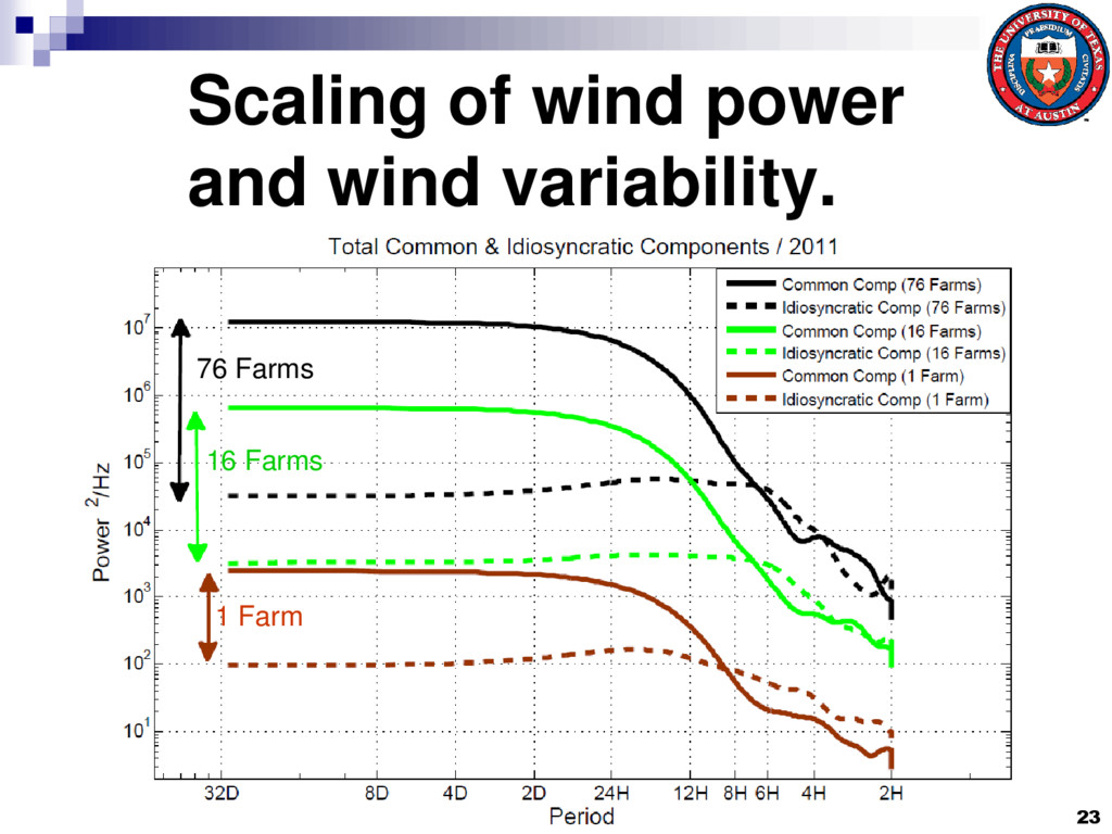
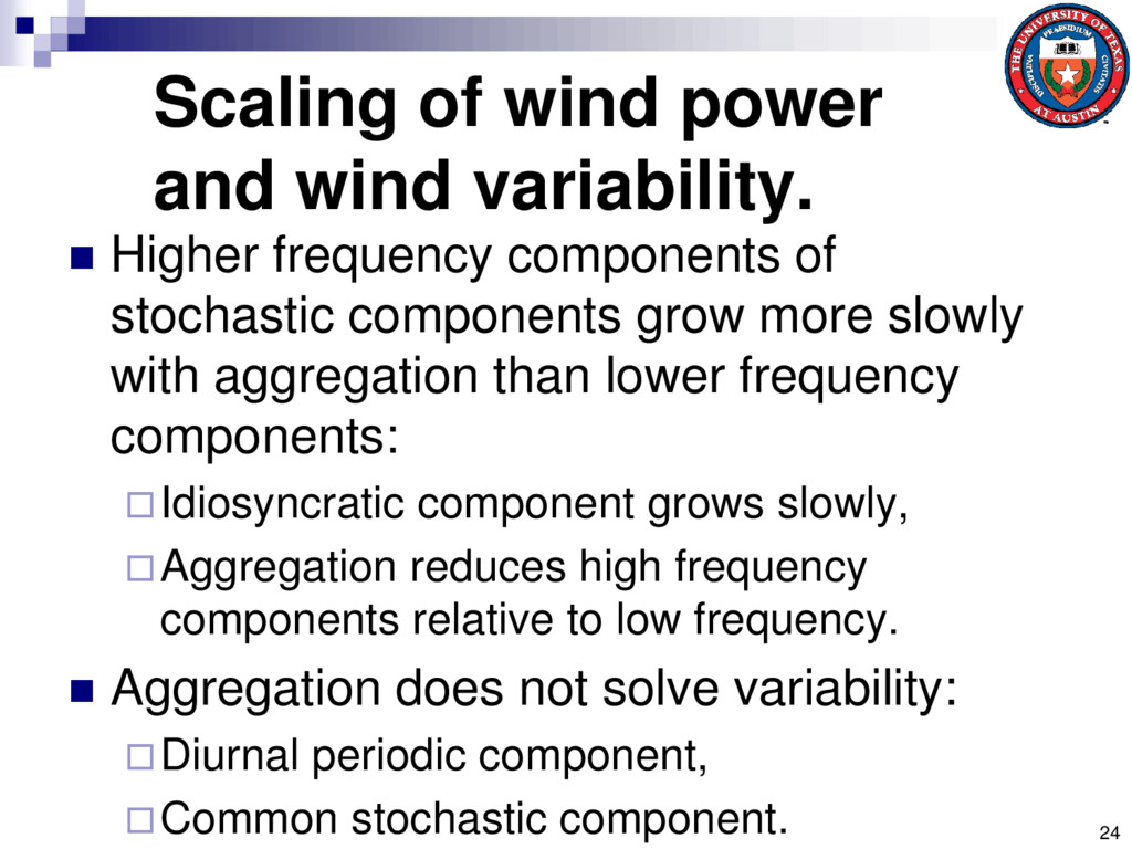
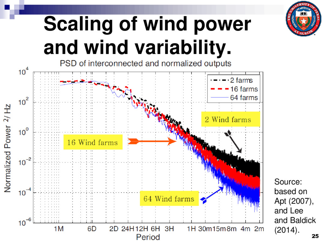
19. Scaling of wind power and wind variability.  Intuitive that aggregating of wind over large areas should reduce relative variability.  However, variability of each component scales differently with aggregation: Periodic:  Scales approximately linearly with capacity, Common:  Effects of underlying (weather) factors tend to add, Idiosyncratic:  Weakly correlated between farms, so grows slowly. 22
20. 23 Scaling of wind power and wind variability. 1 Farm 76 Farms 16 Farms
21. Scaling of wind power and wind variability.  Higher frequency components of stochastic components grow more slowly with aggregation than lower frequency components: Idiosyncratic component grows slowly, Aggregation reduces high frequency components relative to low frequency.  Aggregation does not solve variability: Diurnal periodic component, Common stochastic component. 24
22. Scaling of wind power and wind variability. 25 Source: based on Apt (2007), and Lee and Baldick (2014).
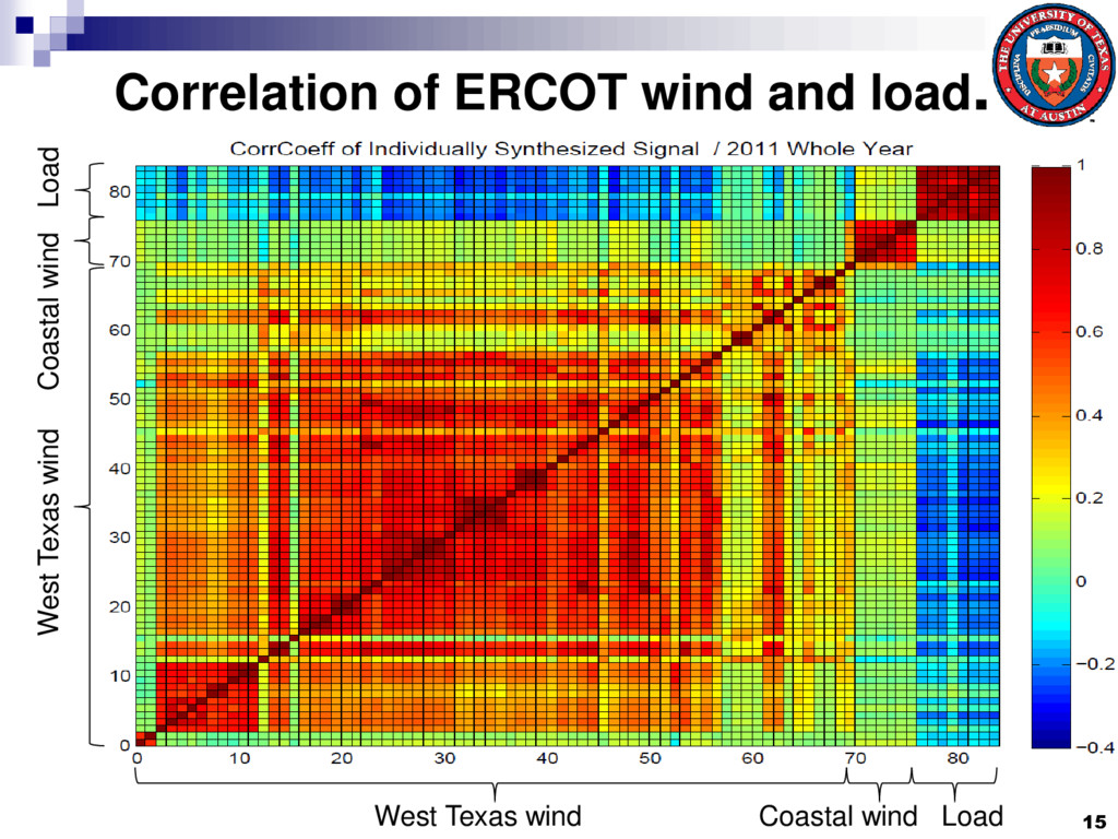
23. Scaling of wind power and wind variability  Echoes observations in Katzenstein, Fertig, and Apt (2010): Most reduction of variability is obtained by aggregating relatively few farms, Still expect significant intermittency in total wind, even aggregating many farms in a region, Intermittency only reduced further by aggregating over geographical scales that span different wind regimes:  Inland and coastal Texas wind. 26
24. Intermittent wind power production. 27
25. Intermittent wind power production. 28
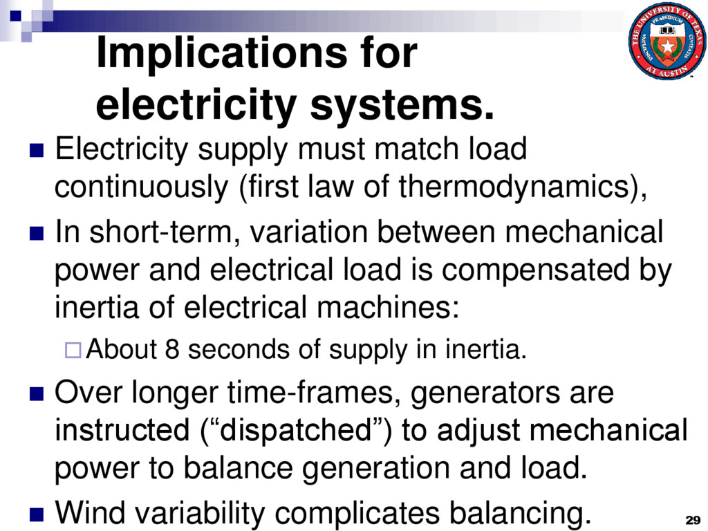
26. Implications for electricity systems.  Electricity supply must match load continuously (first law of thermodynamics),  In short-term, variation between mechanical power and electrical load is compensated by inertia of electrical machines: About 8 seconds of supply in inertia.  Over longer time-frames, generators are instructed (“dispatched”) to adjust mechanical power to balance generation and load.  Wind variability complicates balancing. 29
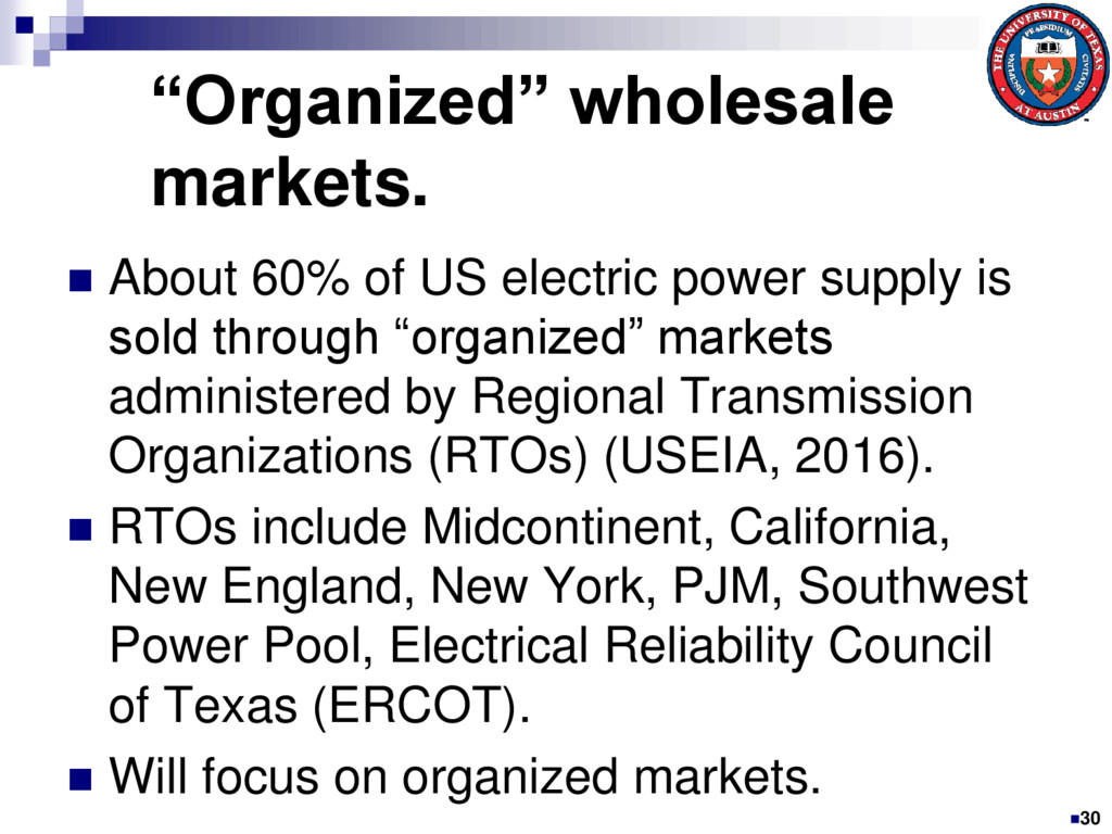
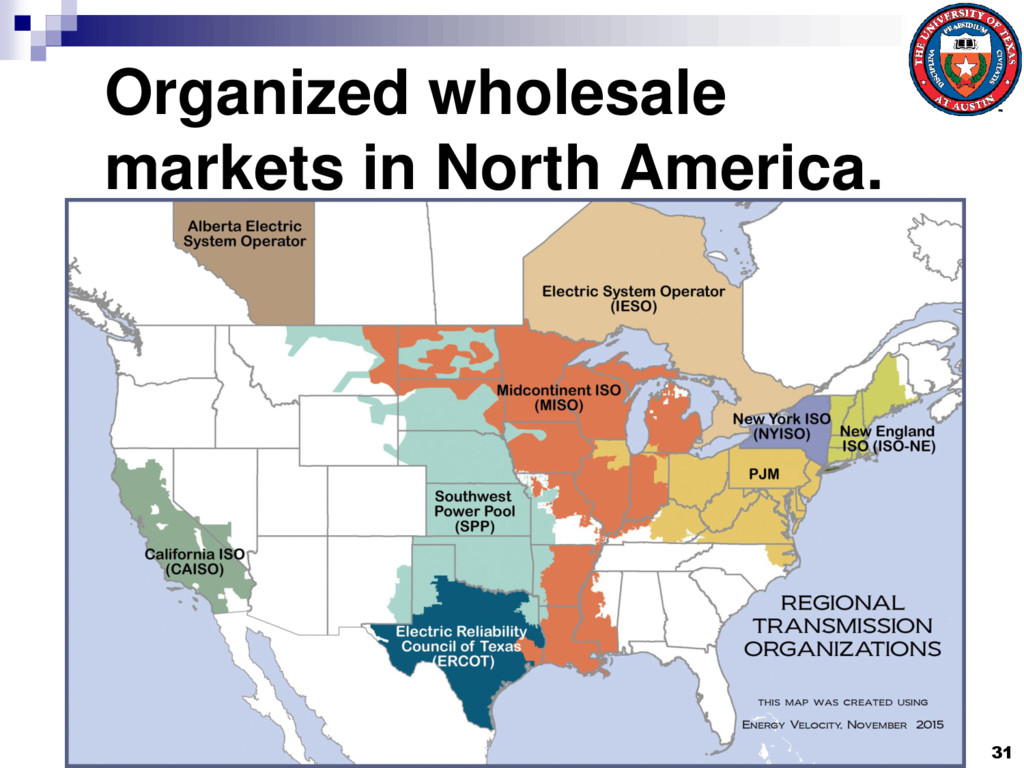
27. “Organized” wholesale markets.  About 60% of US electric power supply is sold through “organized” markets administered by Regional Transmission Organizations (RTOs) (USEIA, 2016).  RTOs include Midcontinent, California, New England, New York, PJM, Southwest Power Pool, Electrical Reliability Council of Texas (ERCOT).  Will focus on organized markets. 30
28. Organized wholesale markets in North America. 31
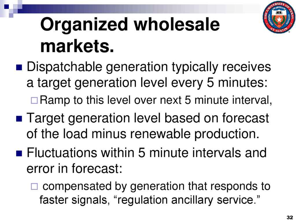
29. Organized wholesale markets.  Dispatchable generation typically receives a target generation level every 5 minutes: Ramp to this level over next 5 minute interval,  Target generation level based on forecast of the load minus renewable production.  Fluctuations within 5 minute intervals and error in forecast:  compensated by generation that responds to faster signals, “regulation ancillary service.” 32
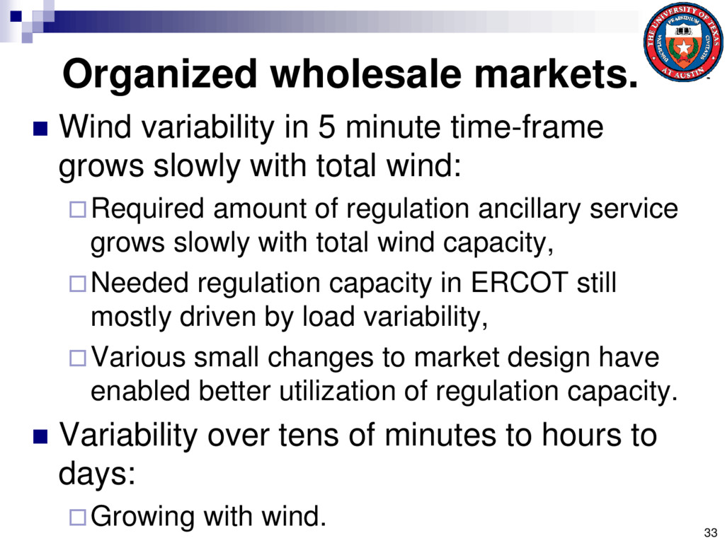
30. Organized wholesale markets.  Wind variability in 5 minute time-frame grows slowly with total wind: Required amount of regulation ancillary service grows slowly with total wind capacity, Needed regulation capacity in ERCOT still mostly driven by load variability, Various small changes to market design have enabled better utilization of regulation capacity.  Variability over tens of minutes to hours to days: Growing with wind. 33
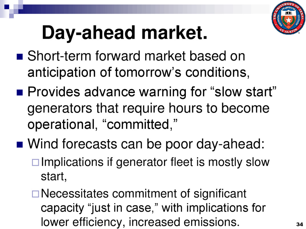
31. Day-ahead market.  Short-term forward market based on anticipation of tomorrow’s conditions,  Provides advance warning for “slow start” generators that require hours to become operational, “committed,”  Wind forecasts can be poor day-ahead: Implications if generator fleet is mostly slow start, Necessitates commitment of significant capacity “just in case,” with implications for lower efficiency, increased emissions. 34
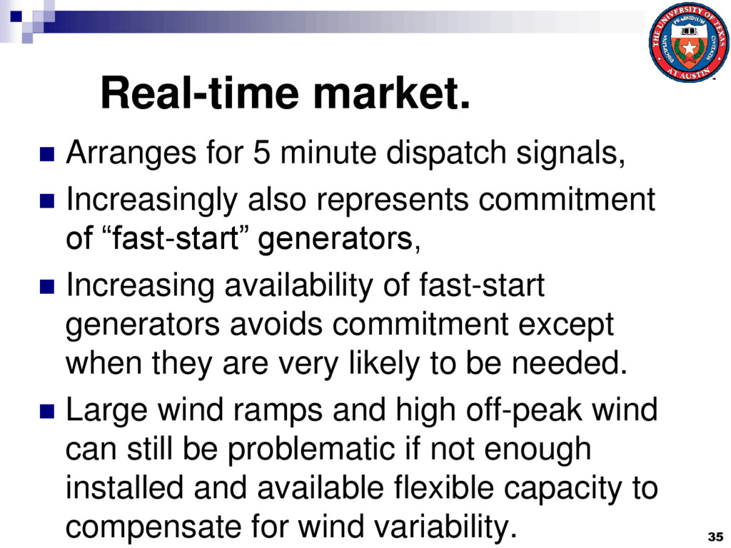
32. Real-time market.  Arranges for 5 minute dispatch signals,  Increasingly also represents commitment of “fast-start” generators,  Increasing availability of fast-start generators avoids commitment except when they are very likely to be needed.  Large wind ramps and high off-peak wind can still be problematic if not enough installed and available flexible capacity to compensate for wind variability. 35
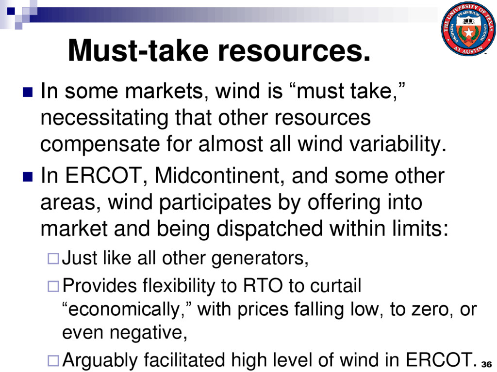
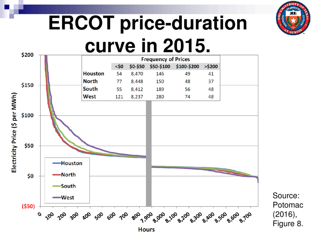
33. Must-take resources.  In some markets, wind is “must take,” necessitating that other resources compensate for almost all wind variability.  In ERCOT, Midcontinent, and some other areas, wind participates by offering into market and being dispatched within limits: Just like all other generators, Provides flexibility to RTO to curtail “economically,” with prices falling low, to zero, or even negative, Arguably facilitated high level of wind in ERCOT. 36
34. Diurnal periodic variation, intermittency, and markets.  West Texas wind has peak production when load is low.  When stochastic wind component adds to periodic peak but load is low, total wind production requires thermal generation to dispatch down or switch off.  In market based approach to integrating wind, this results in low, zero, or even negative prices. 37
35. ERCOT price-duration curve in 2015. Source: Potomac (2016), Figure 8.
36. Conclusion.  Periodic component plus GDFM for stochastic component provides good match to statistics of empirical wind power data: Periodic, common, and idiosyncratic components.  Explains characteristics of aggregated wind production and scope for reduction of variability by aggregation.  Markets with wind will experience times of low or zero prices. 39
37. Current and future work.  Periodic plus GDFM model enables synthesis of wind production and load scenarios: Can be used in transmission and generation planning models.  Analogous models also apply to wind speed and cloud effects: Use with wind farm model to estimate wind power production, Use with cloud-free irradiance to estimate solar production. 40
38. References  USDOE 2016, “Installed Wind Capacity,” Available from: http://www.windpoweringamerica.gov/wind _installed_capacity.asp, Accessed April 27, 2016. 41
39. References  North-American Electric Reliability Corporation, 2015, “NERC Balancing Authorities as of October 1, 2015,” Available from: http://www.nerc.com/comm/OC/RS%20La nding%20Page%20DL/Related%20Files/B A_Bubble_Map_20160427.pdf, Accessed April 30, 2016. 42
40. References  American Wind Energy Association, 2016, “US Wind Industry 2015 Annual Market Update,” Available from: http://awea.files.cms- plus.com/Annual%20Report%20Capacity%20 and%20Generation%202015.pdf, Accessed April 29, 2016.  Potomac Economics 2016, “2015 State of the Market Report for the ERCOT Wholesale Electricity Markets,” Available from www.potomaceconomics.com. 43
41. References.  M. Forni, M. Hallin, M Lippi, and L. Reichlin, “The generalized dynamic factor model: One sided estimation and forecasting,” Journal of the American Statistical Association, 100(471):830-840, 2005  J. Apt, 2007, “The spectrum of power from wind turbines,” Journal of Power Sources,169, 369–374. 45
42. References.  D. Lee and R. Baldick, “Future wind power sample path synthesis through power spectral density analysis,” IEEE Transactions on Smart Grid, 5(1):490-500, January 2014.  W. Katzenstein, E. Fertig, and J. Apt, “The variability of interconnected wind plants,” Energy Policy, 38:4400–4410, 2010. 46
43. References  USEIA 2016, “Today in energy,” Available from: https://www.eia.gov/todayinenergy/detail.cf m?id=790, Accessed April 27, 2016.  Federal Energy Regulatory Commission, 2015, “Regional Transmission Organizations,” Available from: http://www.ferc.gov/industries/electric/indu s-act/rto/elec-ovr-rto-map.pdf, Accessed April 30, 2016. 47