Gridded data with harpIO

Transcript

1. Gridded data with harpIO Alex Deckmyn (RMI), Andrew Singleton (MET Norway), Christoph Zingerle (ZAMG), Bent Hansen Sass (DMI)
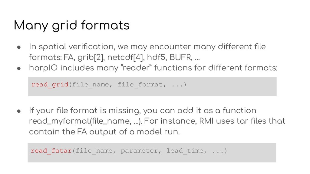
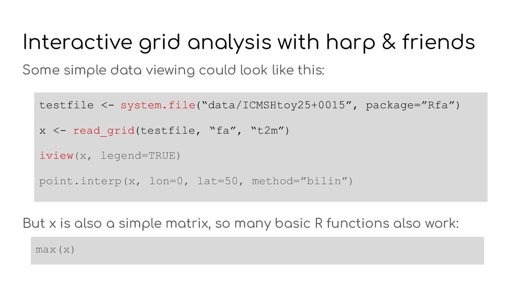
2. Many grid formats • In spatial verification, we may encounter many different file formats: FA, grib[2], netcdf[4], hdf5, BUFR, ... • harpIO includes many “reader” functions for different formats: • If your file format is missing, you can add it as a function read_myformat(file_name, ...). For instance, RMI uses tar files that contain the FA output of a model run. read_grid(file_name, file_format, ...) read_fatar(file_name, parameter, lead_time, ...)
3. Format specific packages To read these formats, we use several packages in the background. Some are standard CRAN packages, others are harp specific and available on github GRIB 1&2: Rgrib2 FA: Rfa (not yet on github) HDF5: h5 (but only ODIM format is fully supported in harpIO) NetCDF: ncdf4
4. Toto, I’ve a feeling we’re not in the Tidyverse anymore.
5. A unified grid format: meteogrid meteogrid (which used to be called geogrid for many years), is a package that implements a unified internal representation for gridded data. It specialises in (and optimises for) weather model data: • multi-dimensional arrays (ensemble members, lead times, vertical levels…) • Projections, grid interpolations, wind fields • Visualisation on maps • Land/sea mask • Original emphasis was on interactive use: data exploration
6. A unified grid format: meteogrid Two main data classes: geodomain and geofield A geodomain represents the grid properties. It is a list with • projection: a proj4 string • nx, ny : grid dimensions • dx, dy : grid resolution • clonlat : central longitude & latitude A geofield is a matrix (or array) with attributes • domain : a geodomain • info : name, variable, time, vert. level, origin...
7. A unified grid format: meteogrid If you have a matrix of data, you turn it into a geofield by adding geodomain (and info) attributes. This is effectively how we would go about implementing new formats. All geofields are equal : meteogrid itself does not know anything about the original data format. You can see the internal list structure of a geodomain by running > dump(“domainname”, file=””)
8. Interactive grid analysis with harp & friends testfile <- system.file(“data/ICMSHtoy25+0015”, package=”Rfa”) x <- read_grid(testfile, “fa”, “t2m”) iview(x, legend=TRUE) point.interp(x, lon=0, lat=50, method=”bilin”) Some simple data viewing could look like this: But x is also a simple matrix, so many basic R functions also work: max(x)
9. Rfa for power users All geofields are equal but … Rfa (and, to a point, it’s sibling Rgrib2) has much more to offer than just decoding 2d fields. • Vertical interpolation (model levels to pressure) • Cross sections • Data encoding, field & file manipulation • Command line tools (bash) via Rscript: This can easily be defined as a bash function. > Rscript -e ‘Rfa::FAopen(“myfile”)$list’
10. FAdec or read_grid(file_format=”fa”,...) ? FAdec(“myfile”, “CLSTEMPERATURE”) vs read_grid(“myfile”,,”t2m”) FAdec() interface is almost 20 years old. It will not change. read_grid() is easier and generic, but sometimes the full Rfa toolbox may be required: extracting & interpreting model levels, “frame” details By the way: did you notice the 2 commas in the read_grid command?
11. What is to come Some more graphical possibilities are in the pipeline: the extra dimensions in geofields can represent many things • Ensemble members -> spread, mean… • Lead time -> animations? • Vertical levels -> cross sections, profiles This will probably be in harpVis, not in meteogrid. But maybe both.