Using your own observations in harpSpatial

An example with the Austrian INCA data

Transcript

1. Getting your own spatial observation Christoph Zingerle (ZAMG), Andrew Singleton(MetNo), Alex Deckmyn (RMI), Bent Hansen Sass (DM)
2. How to get your spatial observation to harp
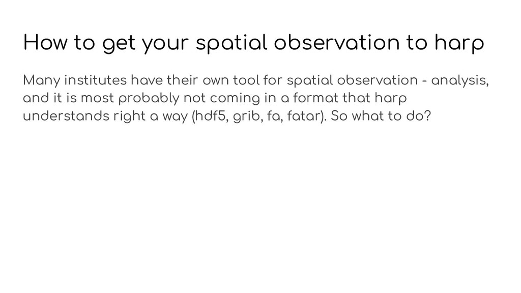
3. How to get your spatial observation to harp Many institutes have their own tool for spatial observation - analysis, and it is most probably not coming in a format that harp understands right a way (hdf5, grib, fa, fatar). So what to do?
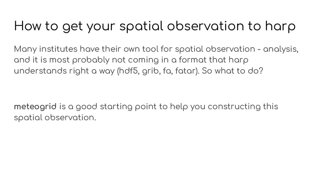
4. How to get your spatial observation to harp Many institutes have their own tool for spatial observation - analysis, and it is most probably not coming in a format that harp understands right a way (hdf5, grib, fa, fatar). So what to do? meteogrid is a good starting point to help you constructing this spatial observation.
5. Gzipped ascii file … What does data look like?
6. What does your data look like
7. What does data look like?
8. library( readr ) library( tidyverse ) # file is gzipped inca <- read_delim( incafile, delim = " ", col_names = FALSE ) %>% dplyr::mutate_all( as.numeric ) How do we read the data
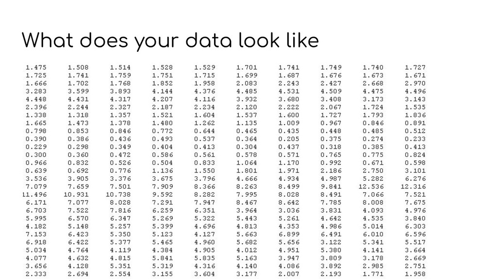
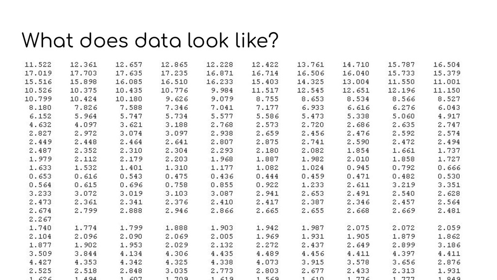
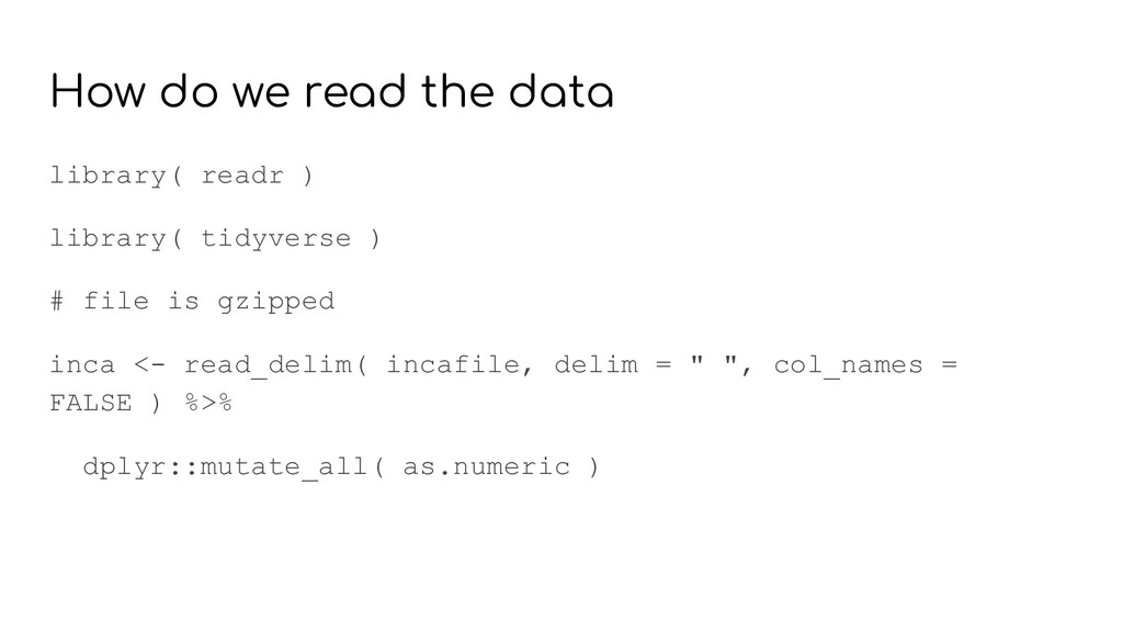
9. Inca output is actually starting in the bottom left, going along the top left line by line - BUT It is written to the ascii file in a really weird way: • Starting bottom left, • writing line by line • but only 10 cols (instead of 701) inca <- c( t( inca ))[!is.na(c( t( inca )))] %>% matrix( nrow = 701 ) Re-arranging needed
10. R is indexing rows first, second is columns so • Transposing the matrix • Make a vector out of it -> get all inca data in one stream • Remove all NA’s • Turn it into a matrix again inca <- c( t( inca ))[!is.na(c( t( inca )))] %>% matrix( nrow = 701 ) Re-arranging needed
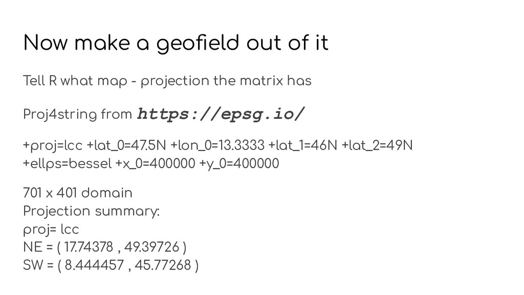
11. Tell R what map - projection the matrix has Proj4string from https://epsg.io/ +proj=lcc +lat_0=47.5N +lon_0=13.3333 +lat_1=46N +lat_2=49N +ellps=bessel +x_0=400000 +y_0=400000 701 x 401 domain Projection summary: proj= lcc NE = ( 17.74378 , 49.39726 ) SW = ( 8.444457 , 45.77268 ) Now make a geofield out of it
12. domainINCA <- structure( list( projection = list( proj = "lcc", lat_0 = 47.5, lon_0 = 13.3333, lat_1 = 46, lat_2 = 49, ellps = "bessel", x_0 = 400000, y_0 = 400000), nx = 701, ny = 401, SW = c(8.444457, 45.772682), NE = c(17.74378, 49.397259) ), class = "geodomain") Now make a geofield out of it
13. inca <- as.geofield( inca, domain = domainINCA, Now make a geofield out of it
14. read_inca <- function( filename ) { ……… return( result ) } How to make it a function
15. To be read by the library( harp ) environment( read_inca ) <- environment( read_grid ) Put it into the environment